

Submitted:
27 March 2025
Posted:
31 March 2025
You are already at the latest version
Abstract
Information processing and control tasks in each unit within a building are typically completed internally, and information processing within a building naturally exhibits distributed characteristics. The insect-intelligent building platform is an intelligent building platform, and the concept of an insect-intelligent building platform adapts to the distributed processing requirements of building information, achieving features such as self-organization and self-adaptation of the intelligent building platform. The microenvironment network serves as a fundamental network that supports the implementation of an insect-intelligent building platform. To quickly solve optimization problems using Particle Swarm Optimization (PSO) under a microenvironment network, update mechanisms for the velocity and position of particles for PSO in the microenvironment are presented, and a Microenvironment-based Particle Swarm Optimization (MPSO) algorithm is proposed in this paper. Experimental results show that, within microenvironment networks, both synchronous and asynchronous implementations of MPSO algorithms can solve optimization problems faster than the PSO algorithm while maintaining a precision similar to that of the PSO algorithm.
Keywords:
Insect-intelligent building platform
; building information process unit
; microenvironment
; PSO
1. Introduction
Building is a general term for buildings and structures. It is a human-made environment designed and constructed to satisfy social life needs by applying known materials and technologies, specific scientific laws, Feng Shui concepts, and aesthetic principles [1]. In general, if the main body of a building is divided into several non-overlapping building spatial units, the building can be considered a composite of all building spatial units [1,2,3,4,5,6,7]. Similarly, if each component of a building facility is considered a building facility unit, the building facility can be regarded as a combination of several facility units [3,4,5,6,7,8,9]. If each building spatial unit and building facility unit in a building are treated as one building unit in the building, the function of the building is a combination of the functions of each building unit, and the maintenance of the building’s function relies on the maintenance of the functions of each building unit [1,4,5,6,7].
For all spatial units within a building, considering whether these spatial units are adjacent, the entire set of spatial units forms a single spatial unit network. Similarly, the building facility can be regarded as a network of these facility units by considering whether its constituent facility units are connected via pipelines, power lines, or other types of lines or pipes. Since each facility unit within a building is deployed within an appropriate spatial unit, by using the criterion of whether a facility unit is deployed within a spatial unit, the entire network of facility units is coupled with the spatial unit network in space. For each building spatial unit and each building facility unit in a building is treated as one building unit, a building can be viewed as a network of interconnected building units [1,3,4,5,6]. Given that building units naturally possess spatial distribution and local characteristics, if the maintenance of a building unit’s function is viewed as an internal information processing task, the building’s information processing process inherently exhibits distributed and localized characteristics [4,5,6,8,9,10,11,12,13,14]. The maintenance of building unit functions is either conducted independently within each unit or carried out within each unit with assistance from adjacent units, with all data processed within each building unit being autonomously collected and handled locally.
Because the information processing required for the maintenance of building functionalities is distributed within each building unit [4,5,6], the maintenance of building functionalities is a combination of the information processing processes within each building unit. In an insect-intelligent building platform [4,5,6,7,8], to meet the information processing and control needs within each building unit, each building unit is equipped with a Building Information Processing Unit (BPU) to satisfy the information processing and control needs of each building unit. All information processing and control tasks within a building unit are completed at last by the BPU deployed in the building unit. When a BPU needs reference data from other building units to complete information processing and equipment control tasks within its local building unit, it can only obtain this data by querying the BPUs in adjacent building units. If each information processing unit deployed within a building unit is viewed as a microenvironment, and it is stipulated that only spatially adjacent microenvironments can exchange information with each other, then the information processing and control network that supports an insect-intelligent building platform consists of a network of microenvironments based on information exchange criteria. All control and information processing tasks within the building were completed within the microenvironment network.
In building units, issues such as intelligent detection of sensor faults, area occupant counting, and tactic selection for environment control are frequently modeled as optimization problems [15,16,17,18,19,20,21,22]. The Particle Swarm Optimization (PSO) algorithm [23] has been widely applied to solve relevant optimization problems within buildings owing to its computational efficiency and simplicity [24,25,26,27,28,29,30,31,32]. In practical applications, the velocity and position update tactics for the particles of the PSO algorithm are generally specified by Equations (1) and (2). In Equations (1) and (2), v(t) represents the velocity of particles, and x(t) represents the position of particles at time t. ω is the inertia factor, c1 is the cognitive (individual) acceleration coefficient, and c2 is the social (global) acceleration coefficient. r1 and r2 are random numbers uniformly distributed in the range [0, 1]. pBest denotes the personal best position of the particles, and gBest denotes the global best position of all particles.
Furthermore, for multi-objective optimization problems in building information processing [35,36,37,38,39], the Niche-based Particle Swarm Optimization (NPSO) algorithm [33,34] has been widely applied to solve multimodal multi-objective optimization problems [35,36,37,38,39]. In the NPSO algorithm, the search space is divided into several regions, and all particles are uniformly distributed across these regions to form subpopulations. The radius of a subpopulation is calculated based on the position of the global best particle and all other particles in the subpopulation. A diversity preservation mechanism is also employed to prevent particles from prematurely converging to local optima within the same region. Thus, the NPSO algorithm effectively balances exploration and exploitation, which are crucial for solving complex optimization problems with multiple objectives and potential solutions.
In an insect-intelligent building platform system, the network for information processing is structured as a microenvironment network based on information exchange criteria across all microenvironments within the building. When the PSO algorithm is employed to solve optimization problems in this microenvironment network, two challenges arise for implementing the PSO algorithm. First, when the computational power of the building’s information processing units is limited, a large number of particles may lead to slow convergence of the PSO algorithm, potentially preventing timely completion of the computational tasks. Conversely, if the number of particles is too low, the PSO algorithm may converge quickly but cannot guarantee solution precision. Secondly, The PSO algorithm is inherently stochastic and requires multiple runs to obtain a satisfactory approximation of the optimal solution. Executing the PSO algorithm multiple times requires more computational power from the processing nodes and additional time for solution attainment.
Because the computational power of each BPU in an insect-intelligent building platform system is generally weak, the performance of solving an optimization problem using the PSO algorithm in a microenvironment network can be enhanced by evenly distributing all particles across each microenvironment by running a PSO algorithm instance with a small number of particles in each microenvironment and exchanging essential computational results among the microenvironments through the network for collaborative computation. This method effectively distributes the optimization requirements based on the PSO algorithm in one microenvironment to each microenvironment node, significantly reducing the computational demands on each microenvironment while simultaneously allowing each microenvironment to approximate the optimal solution to the optimization problem. Consequently, multiple approximate optimal solutions can be rapidly acquired, facilitating the efficient and repeated solving of optimization problems. This study investigates the updating mechanisms for the particle velocity and position of the PSO algorithm in a microenvironment network and presents a Microenvironment-based Particle Swarm Optimization (MPSO) algorithm. The MPSO algorithm is presented in the second section. The third section evaluates the performance of the MPSO algorithm through experimental testing, and the fourth section summarizes the research on the MPSO algorithm.
2. Microenvironment-Based Particle Swarm Optimization Algorithm
In an insect-intelligent building platform, a building is considered a combination of several spatially adjacent building units, each equipped with a BPU. Each BPU represents a microenvironment within the building, and all the microenvironments within the building form a microenvironment network. The microenvironment network is responsible for all building control and information processing tasks. A certain number of sensing and control devices are typically deployed within each building unit, and the BPU located in it is responsible for sensing information and controlling devices in its designated building unit. Because the information processing or control results within a building unit may directly impact adjacent units, BPUs in neighboring units may communicate. Communication is essential for data sharing and collaborative computing. Consequently, in the microenvironment network, microenvironments that are spatially adjacent and require communication are considered neighboring microenvironments. Figure 1 illustrates the topology of a microenvironment network. In Figure 1, a gray dot represents one microenvironment node, and one edge indicates the adjacency between the two microenvironments. Logically, all microenvironment nodes were arranged in a 4-row by 5-column format, totaling 20 microenvironment nodes, as shown in Figure 1. In the microenvironment network illustrated in Figure 1, each node can only communicate and exchange data with its directly adjacent nodes. Any two non-adjacent microenvironment nodes cannot communicate directly or exchange data.
Generally, in the PSO algorithm, a particle represents a feasible solution to the corresponding optimization problem. When the PSO algorithm is implemented in a microenvironment network, each particle must be assigned to a microenvironment, and each microenvironment may contain several particles (for simplicity, the number of particles in each microenvironment can be the same.). The following assumptions are required to implement the PSO algorithm in a microenvironment network:
- 1)
- There are several particles in each microenvironment.
- 2)
- For any given microenvironment, gBestL denotes the historical best position of all particles in the microenvironment.
- 3)
- For a particular microenvironment with m neighboring microenvironments, gBestLi denotes the best position of all particles in the ith neighboring microenvironment, and gBestA is defined according to Equation (3). In the microenvironment-based PSO algorithm, for any particle in a given microenvironment with position x(t) and velocity v(t) at time t, the velocity v(t+1) and position x(t+1) at time t +1 are determined using Equations (4) and (2), respectively. Equation (3) is known as the data exchange tactic in the microenvironment-based PSO algorithm, whereas Equations (4) and (2) describe the update tactic of the particle position within the algorithm.
A full description of the MPSO (Microenvironment-based Particle Swarm Optimization) algorithm is presented in Algorithm 1. In Algorithm 1, the fitness value of each particle is used to evaluate the quality of the particle’s position; the smaller the fitness value, the better the particle’s position. Fitness function fun () is used to calculate the fitness value of a particle, where the position of the particle serves as the independent variable for the function. As shown in Algorithm 1, the following three constraints are imposed:
- 1)
- Within each microenvironment, a small number of particles serves as a population that can independently execute a PSO algorithm instance, which adapts the characteristics of the microenvironment’s information.
- 2)
- A microenvironment can exchange information with its neighboring microenvironments. Those microenvironments can query the position information of historically optimal particles within each other’s neighboring microenvironments.
- 3)
- Non-adjacent microenvironment nodes could not exchange information in the microenvironment network.
|
Algorithm 1: Microenvironment-based PSO algorithm (MPSO) Input: n, number of particles in a microenvironment; d, the dimension of position for each particle; c1 and c2, learning factors; ω, inertial factor; maxN, maximum number of iterations; fun, fitness function; pNeighbor, the list of neighboring microenvironments Output: gBestL, the historical optimal position of all local particles in the microenvironment
|
Let gBest be the best position of all particles within the microenvironment network at time k. For any microenvironment within the microenvironment network, fun(gBestL)≥fun(gBestA)≥fun(gBest). In the MPSO algorithm, the fitness values of the particle positions within the microenvironment can converge to the fun(gBest) after a finite number of iterations, because the velocity and position of each particle within any microenvironment are updated using Equations (4) and (2). Although the global best position gBest may not appear in each microenvironment, according to the connectivity characteristics of the microenvironments in the microenvironmental network and Equation (3), the global best position gBest can be transmitted to any microenvironment within a finite number of iterations because any two microenvironments can exchange information within a finite number of steps in the microenvironmental network. In extreme cases, let all m microenvironments in the microenvironmental network be lined in a row; the first microenvironment is labeled with A, and the last microenvironment is labeled with B. If the optimal position, gBest is the local optimal position within microenvironment A, then at most within m-1 iterations, the local optimal position in microenvironment B will be better than the local optimal position in microenvironment A m-1 iterations before, that is, better than the global optimal position m-1 iterations before. The data exchange strategy specified in Equation (3) can propagate the global best position gBestto each microenvironment in the microenvironmental network. The fact that gBest can be transmitted to each microenvironment implies that the local best positions, gBestL of each microenvironment are within a finite number of steps from the global best position. This is manifested as a slight difference in the fitness values of gBestL for each microenvironment when Algorithm 1 has finished its operation.
In Algorithm 1, Step 5 determines whether Steps 6–13 continue to iterate by checking whether the iteration count k is less than the maximum iteration count maxN. If the condition “k <= maxN” in step 5 is revised to “k<=maxN and fun(gBestL) <= goalExpect,” Algorithm 1 can control whether Steps 6 to 13 continue to iterate based on the condition that whether the iteration count k is less than maxN, and the performance of the global best position of all local particles, gBestL is better than goalExpect, the expected performance. For the modified iteration control condition, if the maximum iteration count maxN is set to a considerable value, the loop for the update of gBestL is controlled by the condition that whether the performance of gBestL is better than the expected performance, goalExpect.
For Algorithm 1, when gBestL, the global best position of all local particles, is calculated at the k iteration, if step 6 requires that the historical best position gBestL of each neighboring microenvironment must correspond to the k iteration, algorithm 1 is the synchronous form of the MPSO algorithm. On the other hand, if Step 6 only requires the historical best position gBestL of each neighboring microenvironment from the most recent iteration, Algorithm 1 is the asynchronous form of the MPSO algorithm.
3. Experiment Results and Analysis
To verify the effectiveness of the MPSO algorithm, six benchmark functions listed in Table 1 were used to evaluate the performance, such as the time consumption and precision of Algorithm 1 in our experiment. In addition, the influence of different communication methods and microenvironment network topologies on the performance of Algorithm 1 is tested. Figure 2 shows the shapes of those six benchmark functions when the number of independent variables d is 2. In the experiment for Algorithm 1 executed in each microenvironment, n=20, d=2, c1=2, c2=2, ω=0.8, where n is the local particle number, d is the dimension of the particle position, c1 and c2 are learning factors, and ω is the inertia factor. The fitness function fun (), the maximum number of iterations maxN, and the neighbor microenvironment node list pNeighbor were determined based on the optimization problem, the iteration termination condition, and the topology of the microenvironment network.
The topology of the microenvironment network used in the experiment is shown in Figure 3, which corresponds to the distribution of spatial units of the Anhui Province Key Laboratory of Intelligent Building and Building Energy Saving [40]. When an optimization problem is solved using the PSO algorithm, the solution obtained by a single run of the PSO algorithm is typically a candidate solution of the optimization problem since PSO is a stochastic search algorithm. To find the optimal solution to an optimization problem, the PSO algorithm must be applied multiple times, and the candidate solution with the best precision is chosen as the optimal solution. Because there are 12 microenvironments in the microenvironment network illustrated in Figure 3, the experiment first treated these 12 microenvironments as 12 independent computing environments in which the PSO algorithm independently solved the extremum of benchmark functions when the PSO algorithm is used to independently solve the extremum of benchmark functions in each computing environment, n=240, d=2, c1=2, c2=2, and ω=0.8.
The time consumed and convergence precision of the PSO algorithm in the 12 nodes microenvironment network shown in Figure 2 when maxN=200 for the extremum of each benchmark function solving are listed in Table 2. According to Table 2, when the PSO algorithm is repeatedly used to solve the extremum of the benchmark functions, the performance of the extremum candidate values for all benchmark functions, except the Schwefel function, exceeds the desired performance of 1e-05, and the extremum performance of the Schwefel function can reach the 1e-05 level. Additionally, the significant differences between the values in the “maximum” and “average” of precision columns shaded in gray and the corresponding “minimum” values of precision in Table 2 indicate the necessity of running the PSO algorithm multiple times for optimization problem solving. Similarly, Table 3 lists the time, convergence precision, and maximum number of iterations for independently solving the extremum of each benchmark function using the PSO algorithm in 12 microenvironments with maxN=200 and goal precision=1e-5. Table 4 lists the time and convergence precision for independently solving the extremum of each benchmark function using the PSO algorithm in 12 microenvironments with goal precision=1e-5 and maxN=20,000 to prevent excessively long computation times.
Given that the experimental data in Table 2 show that the performance of the PSO algorithm for the extremum of the Schwefel function solving is greater than 1e-5, the goal performance for the minimum value of the Schwefel function in Table 3 is 1e-04. For comparison, the goal performance for the minimum value of the Schwefel function in Table 4 is 1e-5. Table 3 and Table 4 show that when the PSO algorithm is repeatedly used to solve the extremum of the benchmark functions, the performance of the minimum value of all benchmark functions, excluding the Schwefel function, surpasses 1e-5, which is the goal performance. In contrast, the performance of the Schwefel function’s minimum value surpasses 1e-4. According to the minimum precision in Table 2, Table 3 and Table 4, it can be concluded that the PSO algorithm can effectively obtain the extremum of all benchmark functions. Furthermore, the significant differences between the shaded “maximum” and “average” values of precision and the corresponding “minimum” values of precision in Table 2, Table 3 and Table 4 also highlight the necessity of running the PSO algorithm multiple times.
By comparing the data in the “Minimum” column of the precision part and the “Minimum,” “Maximum,” “Average,” and “Total” columns of the time part for the Schwefel row in Table 2, Table 3 and Table 4, respectively, it can be observed that when the minimum of the Schwefel function is solved using the PSO algorithm, as shown in the data in Table 2 and Table 3, the performance of the feasible solutions obtained by the PSO algorithm can quickly surpass 1e-4. However, by comparing the data in Table 4, even with continued iterations, the precision of the feasible solutions obtained by the PSO algorithm remained challenging, reaching 1e-5 within 20,000 iterations.
With the microenvironment network of 12 microenvironment nodes illustrated in Figure 3, the experiment further tested the time and precision performance of the synchronous MPSO algorithm for the extremum search of each benchmark function. The experimental results for maxN=200 are presented in Table 5. Table 6 presents the experimental results for maxN=200 and 1e-05 as the goal precision, where maxN is the maximum number of iterations. Table 7 lists the experimental results for 1e-05 as the goal precision. In Table 6 and Table 7, the goal precision for the minimum Schwefel function is 1e-04. In the experiment, the number of particles in the PSO algorithm was set to 240 with 20 particles in each microenvironment. Based on the minimum precision values listed in Table 5, Table 6 and Table 7, it can be concluded that the synchronous MPSO algorithm can effectively determine the extremum of all benchmark functions. Furthermore, by comparing the summary of the time part in Table 2, Table 3 and Table 4 with the maximum time part in Table 5, Table 6 and Table 7, it is evident that when an optimization problem must be solved multiple times under the same convergence conditions to obtain some candidate solutions, and the optimal solution for the desired optimization problem is selected from those multiple candidates, the synchronous MPSO algorithm consistently requires much less time than the PSO algorithm.
Using the microenvironment network of the 12 nodes microenvironment illustrated in Figure 3, the experiment further tested the time and precision performance of the asynchronous MPSO algorithm for the extremum of each benchmark function. The experimental results for maxN=200 are presented in Table 8. Table 9 presents the experimental results for maxN=200 and 1e-05 as the goal precision, where maxN is the maximum number of iterations. Table 10 lists the experimental results for 1e-05 as the goal precision. In Table 8 and Table 9, the goal precision for the minimum Schwefel function is 1e-04. In the experiment, the number of particles in the PSO algorithm was set to 240 with 20 particles in each microenvironment. Based on the minimum precision values listed in Table 8, Table 9 and Table 10, it can be concluded that the asynchronous MPSO algorithm can effectively determine the extremum of all benchmark functions. Furthermore, by comparing the summary of the time part in Table 2, Table 3 and Table 4 with the maximum time part in Table 8, Table 9 and Table 10, it is evident that when an optimization problem must be solved multiple times under the same convergence conditions to obtain some candidate solutions, and the optimal solution for the desired optimization problem is selected from those multiple candidates, the asynchronous MPSO algorithm consistently requires much less time than the PSO algorithm. By comparing the precision and time data in Table 5, Table 6 and Table 7 and Table 8, Table 9 and Table 10, it can be observed that the asynchronous MPSO algorithm generally achieves slightly lower precision in approximating the optimal solutions of all benchmark functions compared to the synchronous MPSO algorithm, but it requires more time. The synchronous MPSO algorithm performed better than the asynchronous MPSO algorithm in solving the optimal solutions of the benchmark functions.
The topology of the microenvironment network for the performance data of the MPSO listed in Table 5, Table 6, Table 7, Table 8, Table 9 and Table 10 is illustrated in Figure 3, which is an actual microenvironment network deployed in the Anhui Provincial Key Laboratory of Intelligent Buildings and Building Energy Saving. It is consistent with the spatial unit distribution of the laboratory. Furthermore, to test the robustness of the MPSO algorithm, four different microenvironmental network topologies were used, and the microenvironment network had 12 microenvironment nodes. The topologies of the four microenvironmental networks are shown in Figure 4. These topologies were used to evaluate the performance of the synchronous MPSO algorithm in solving the extremum of all benchmark functions. The goal performance for the Schwefel function was set to 1e-04, whereas that for the other benchmark functions was set to 1e-05.
Four microenvironment networks are shown in Figure 4. Each microenvironment network shown in Figure 4 has 12 microenvironment nodes, each of which has a unique topology, such as line, ring, full, or random topology. In the line microenvironment network, except for the first and last nodes, each node has two neighbors, and each node can only communicate with its adjacent neighbors. In a ring microenvironment network, each node has two neighboring nodes, and all nodes form a closed loop. Each microenvironment node can communicate with its neighbors only in a ring microenvironment network. In a full microenvironment network, each microenvironment node can communicate with each other nodes. The random topology of a microenvironment network is a randomly generated connected graph with 12 nodes. When generating a random topology, each node must have at least one neighbor and no more than six neighbors. This corresponds to the spatial structure of a building, where each spatial unit can have up to six neighbors located in directions such as up, down, left, right, front, and back.
To test the performance of the synchronous MPSO algorithm for the extremum of all benchmark functions solved across the four different microenvironment network topologies, in further experiments, the synchronous MPSO algorithm was executed in each microenvironment, and n=20, d=2, c1=2, c2=2, ω=0.8, where n is the local particle number, d is the dimension of the particle position, c1 and c2 are the learning factors, and ω is the inertia factor. Furthermore, the goal performance for each benchmark function, except for the Schwefel function, was set to 1e-05, and the goal precision for the Schwefel function was 1e-04. Meanwhile, maxN, the maximum number of iterations, was set to 20,000. The fitness function fun() was defined as each of the benchmark functions, and the list of neighboring microenvironment nodes pNeighbor was determined based on the microenvironment network topologies shown in Figure 4.
With those four microenvironment networks illustrated in Figure 4, the experiment further tested the time and precision performance of the synchronous MPSO algorithm for solving the extremum of each benchmark function. The time and precision data are listed in Table 11, Table 12, Table 13 and Table 14. The precision of the synchronous MPSO algorithm in solving the extremum of all benchmark functions in each microenvironment network topology can reach this goal. Furthermore, by comparing the Total Time data in the “Total Time” column of Table 4 with the maximum time data in the “Max Time” column of Table 11, Table 12, Table 13 and Table 14 to solve the extremum of each benchmark function, it is evident that when the best solution of an optimization problem needs to be selected from some candidate solutions, the time consumed by the synchronous MPSO algorithm is less than the time consumed by the PSO algorithm.
In the current research and application of building intelligence and building energy efficiency, to complete some common tasks, such as fault diagnosis and optimization, fine-grained environmental control, energy efficiency optimization, occupant localization, and occupant behavior analysis, the reconstruction of the temperature field in building spatial units based on temperature monitoring data from a few interesting locations is a common optimization task. The PSO algorithm is frequently employed to optimize the temperature field reconstruction model.
In the following experiment, a feedforward neural network with one hidden layer was used as the reconstruction model of the temperature field for building spatial units. This model had an input layer with two input neurons, a hidden layer with two hidden neurons, and an output layer with one output neuron. The input layer was fully connected to the hidden layer, and the hidden layer was fully connected to the output layer. Each neuron in the hidden and output layers had a bias. The active function for each hidden layer neuron is a hyperbolic tangent function , and the active function for each output layer neuron is the linear function . During data collection, only five temperature monitoring points were arranged in the northeast, southeast, southwest, northwest, and center of the building spatial unit. The volume of the collected data was minimal, whereas the spatial span was large. Therefore, it is not advisable to train the feedforward neural network using the BP algorithm directly. Hence, the model parameters (weights of all neuron connections) were trained using the PSO algorithm. The performance of the MPSO algorithm for the temperature field reconstruction model training in the microenvironment topology illustrated in Figure 3 was tested in the following experiment. For comparison, the performance of the PSO algorithm for training the temperature field reconstruction model was also tested in the following experiment. Information such as computation time, precision, and number of iterations of the PSO, Synchronous MPSO, and Asynchronous MPSO algorithms for the temperature field reconstruction model training are given in Table 15, and the temperature fields reconstructed by the temperature field reconstruction model trained by the PSO, Synchronous MPSO, and Asynchronous MPSO algorithms are shown in Figure 5. In the experiment, the goal precision for the PSO, Synchronous MPSO, and Asynchronous MPSO algorithms was set to 1e-08, and the maximum number of iterations (maxN) was set to 2000. The number of particles in the PSO algorithm was 600, whereas the number of particles in each microenvironment for both the synchronous and asynchronous MPSO algorithms was 50. To collect data for the information in Table 15, the PSO algorithm independently optimized the temperature field reconstruction model in 12 microenvironments. By contrast, the synchronous and asynchronous MPSO algorithms optimized the model in the same 12 microenvironments.
From the data in the “Min” column of the precision part in Table 15, it can be asserted that the PSO, synchronous MPSO, and asynchronous MPSO algorithms can effectively optimize the temperature field reconstruction model. Moreover, by comparing the data in the “Min,” “Max,” and “mean” columns of the precision part in Table 15, it is evident that when the PSO algorithm is used to optimize the temperature field reconstruction model, the precision of the model fluctuates significantly upon convergence. In contrast, when the synchronous and asynchronous MPSO algorithms were used to optimize the temperature field reconstruction model, the precision of the model remained stable. The similarity in the contour plots of the temperature fields reconstructed by the models using the three methods, as shown in Figure 5, also indicates that these algorithms can optimize the temperature field reconstruction model. Furthermore, from the time taken for the optimization of the temperature field reconstruction model in Table 15, the maximum optimization time for the synchronous and asynchronous MPSO algorithms was significantly less than the total time taken by the PSO algorithm when it was repeated 12 times (the total time was 12 times the average value). The maximum time required by the synchronous MPSO algorithm was also less than that of the asynchronous MPSO algorithm. The synchronous MPSO algorithm is more suitable for optimizing the temperature field reconstruction model.
All experiments were completed on a microenvironment network platform with 12 PCs as microenvironment nodes. Each PC had one Intel Core i7 processor and 16GB of DDR4 memory. A microenvironment network platform was constructed based on the local area network. All PCs were purchased from the same vendor in the same batch to ensure consistent performance metrics. The operating system for each microenvironment was Linux Fedora fc38.x86_64. Each algorithm was implemented using Python programming language. MariaDB 10.5.21 for Linux (x86_64) was deployed to store the local data in each microenvironment.
4. Conclusion and Future Work
By considering the distribution of building spatial units, the diversity of facilities, and the spatial distribution of facility components within buildings, the information processing processes in buildings naturally possess distributed characteristics. The inherent distribution characteristics of building information processing are referenced in the context of an insect-intelligent building platform. Distributed sensors and the processing of building information are achieved by deploying building information processing units within building units equipped with sensors, control, and information processing capabilities. This insect-intelligent building platform technology offers a new perspective with self-organizing and self-adaptive features for intelligent building operation, maintenance, and building energy efficiency management. The microenvironment-based particle swarm optimization (MPSO) algorithm was designed by considering the foundational network of an insect-intelligent building platform as a microenvironment network. The MPSO algorithm was tailored to the structure of the microenvironment network. The MPSO algorithm integrates the computational resources distributed across various building information units, providing a rapid solution approach based on evolutionary computation principles for solving optimization problems within an insect-intelligent platform. Because the MPSO algorithm requires the collaboration of microenvironment nodes within a microenvironment network to solve optimization problems, this study tested the computation time and precision of the synchronous and asynchronous forms of the MPSO algorithm in solving optimization problems. The computation time and precision are compared with the computation time and precision of the PSO algorithm for the same optimization problem. The experimental results show that both the synchronous and asynchronous MPSO algorithms can quickly solve the given optimization problems, while the performance is equivalent to that of the PSO algorithm.
To obtain multiple candidate solutions simultaneously, the MPSO algorithm iteratively updates the positions of particles through collaboration among adjacent microenvironments. The best performing candidate solution was selected as the optimal solution. This method for obtaining the optimal solution does not consider the possibility of microenvironments experiencing faults or some cases, such as a microenvironment node having to exit the collaborative computation for some emergency tasks. The effect of specific microenvironments exiting collaborative computation on the performance of the MPSO algorithm is an interesting issue. Furthermore, the influence of key nodes in the microenvironment network forced to exit collaborative computation on the performance of the MPSO algorithm is another critical issue that requires attention.
If an optimization problem is solved using the PSO algorithm in a microenvironment network, it can also be achieved by assigning appropriate subtasks to each microenvironment node and aggregating the results of all subtasks at the node that issued the tasks to find the current best solution to the optimization problem. This process is iteratively updated to obtain the overall optimal solution. With this approach, the solution for the optimization problem obtained by the PSO algorithm is only presented in the microenvironment that starts the solving process of the optimization problem. The performance of the MPSO algorithm implemented in this manner is worth investigating. Furthermore, the identification of microenvironment network topologies that support this implementation method and the calculation of the microenvironment network diameter are topics that merit further research.
Author Contributions
Z.Z., H.C.: Methodology, Conceptualization, Validation. S.X., P.W.: Methodology, Software, Writing—original draft. H.C., S.Z.: Methodology, Visualization, Writing—review and editing. All authors have read and agreed to the published version of the manuscript.
Funding
Please add: This work was partially supported by the Discipline (Major) Top-notch Talent Academic Funding Project of Anhui Provincial University and College under Grant gxbjZD2021067 and gxyq2022030, the Innovative Leading Talents Project of Anhui Provincial Special Support Program under Grant [2022]21, the Key Project of Natural Science Research of Universities of Anhui Province under Grant 2024AH050246, the director foundation of the Anhui Province Key Laboratory of Intelligent Building & Building Energy Saving under Grant IBES2022ZR01 and IBES2024ZR02.
Data Availability Statement
The original contributions presented in this study are included in the article. Further inquiries can be directed to the corresponding author.
Acknowledgments
The authors would like to acknowledge the Discipline (Major) Top-notch Talent Academic Funding Project of Anhui Provincial University and College under Grant gxbjZD2021067 and gxyq2022030, the Innovative Leading Talents Project of Anhui Provincial Special Support Program under Grant [2022]21, the Key Project of Natural Science Research of Universities of Anhui Province under Grant 2024AH050246, the director foundation of the Anhui Province Key Laboratory of Intelligent Building & Building Energy Saving under Grant IBES2022ZR01and IBES2024ZR02.
Conflicts of Interest
The authors declare no conflicts of interest.
References
- ShenQi. Studies on Architecture of DecentralizedSystem in Intelligent Building[D], Tsinghua University, 2015.
- ZHAO, Tianyi; GUAN, Xulei; CHEN, yifan; HUA, Pengmin. Study on Information Model of Building Spatial Unit for Distributed Architecture[J], Building Science,2023,39(08):233-240. [CrossRef]
- Zhao, Qianchuan; Xia, Li; Jiang, Ziyan. Project report: new generation intelligent building platform techniques, Energy Informatics, 2018.12,1(1):12-16. [CrossRef]
- Zhao, Qianchuan; Jiang, Ziyan. Insect intelligent building (I2B): A New Architecture of Building Control Systems Based on Internet of Things (IoT), Advances in Intelligent Systems and Computing, 2019, 890:457-466. [CrossRef]
- Tian Xing; Hu Yan; Kailai Sun; Yifan Wang; Xuetao Wang; Qianchuan Zhao, Honeycomb: An open-source distributed system for smart buildings, Patterns,2022.11,3(11). [CrossRef]
- Zhang, Zhen-Ya; Fang, Bo; Wang, Ping; Cheng, Hong-Mei. A Local Area Network-Based Insect Intelligent Building Platform. International Journal of Pattern Recognition & Artificial Intelligence. 2023;37(2):1-16. [CrossRef]
- Jiang Ziyan, Dai Yunchuang, Jiang Yi. Swarm intelligent building automation system[J], Heating Ventilating & Air Conditioning, 2019.11,49(11):2-17.
- Jiang, Ziyan; Dai, Yunchuang, A decentralized, flat-structured building automation system. Energy Procedia, 2017, 122:68-73. [CrossRef]
- LIU Xiguang, XIE Liqiang, YANG Qiliang, XING Jianchun, JIANG Ziyan, ZHAO Qianchuan. Simulation Experiment Study on Firefighting System under the Insect Intelligent Building Platform[J], Building Science, 2020,36(04):149-154. [CrossRef]
- Diao, Pei-Huang; Shih, Naai-Jung. BIM-Based AR Maintenance System (BARMS) as an Intelligent Instruction Platform for Complex Plumbing Facilities. Applied Sciences. 2019.4; 9(8). [CrossRef]
- Laohaviraphap, Neeraparng; Waroonkun, Tanut. Integrating Artificial Intelligence and the Internet of Things in Cultural Heritage Preservation: A Systematic Review of Risk Management and Environmental Monitoring Strategies, Buildings, 2024,14(12), 3979. [CrossRef]
- Hosamo, HH; Svennevig, PR; Svidt, K; Han, DG; Nielsen, HK. A Digital Twin predictive maintenance framework of air handling units based on automatic fault detection and diagnostics, Energy and Buildings, 2022.4,261. [CrossRef]
- Jiajie Xu, Dejuan Li, Wei Gu, Ying Chen, UAV-assisted task offloading for IoT in smart buildings and environment via deep reinforcement learning, Building and Environment, 2022.8, 222. [CrossRef]
- Zhiwei Li, Jili Zhang, Song Mu, Passenger spatiotemporal distribution prediction in airport terminals based on insect intelligent building architecture and its contribution to fresh air energy saving, Sustainable Cities and Society, 2023.10, 97:104772. [CrossRef]
- Haixia Li, Yu Guo, Huajian Zhao, Yang Wang, David Chow, Towards automated greenhouse: A state of the art review on greenhouse monitoring methods and technologies based on internet of things, Computers and Electronics in Agriculture, 2021.12,191:106558. [CrossRef]
- Qaisar, Irfan; Sun, Kailai; Zhao, Qianchuan; Xing, Tian; Yan, Hu. Multi-Sensor-Based Occupancy Prediction in a Multi-Zone Office Building with Transformer. Buildings 2023.8, 13(8): 2002. [CrossRef]
- Li, Cui, Ping Lu, Weiran Zhu, Han Zhu, and Xinmin Zhang. Intelligent Monitoring Platform and Application for Building Energy Using Information Based on Digital Twin, Energies, 2023.10, 16(19): 6839. [CrossRef]
- H. Li, J. Xu, Q. Zhao and S. Wang, Economic Model Predictive Control in Buildings Based on Piecewise Linear Approximation of Predicted Mean Vote Index, IEEE Transactions on Automation Science and Engineering, 2023.6. [CrossRef]
- N. Ahmad, M. Egan, J. -M. Gorce, J. S. Dibangoye and F. Le Mouël, Codesigned Communication and Data Analytics for Condition-Based Maintenance in Smart Buildings, IEEE Internet of Things Journal, 2023.9, 10(8):15847-15856. [CrossRef]
- Piras, Giuseppe; Muzi, Francesco; Tiburcio, Virginia Adele. Digital Management Methodology for Building Production Optimization through Digital Twin and Artificial Intelligence Integration, Buildings, 2024.7, 14(7): 2110. [CrossRef]
- Hosamo, HH; Svennevig, PR; Svidt, K; Han, DG; Nielsen, HK, A Digital Twin predictive maintenance framework of air handling units based on automatic fault detection and diagnostics, Energy and Buildings, 2022.4, 261:111988. [CrossRef]
- Kailai Sun, Qianchuan Zhao, Jianhong Zou, A review of building occupancy measurement systems, Energy and Buildings, 2020.6, 216:109965. [CrossRef]
- Kennedy, James; Eberhart, Russell. Optimization Particle Swarm[C]//Proceedings of the 1995 IEEE International Conference on Neural Networks, 1995.8, 4:1942-1948, Washington DC, 1995, IEEE, Piscataway, NJ, USA.
- Malik S, Kim D. Prediction-Learning Algorithm for Efficient Energy Consumption in Smart Buildings Based on Particle Regeneration and Velocity Boost in Particle Swarm Optimization Neural Networks. Energies. 2018.5, 11(5):1289. [CrossRef]
- Wenqiang Jing, Junqi Yu, Wei Luo, Chujun Li, XinYi Liu, Energy-saving diagnosis model of central air-conditioning refrigeration system in large shopping mall, Energy Reports, 2021.11,7:4035-4046. [CrossRef]
- Guo-Feng Fan, Ya Zheng, Wen-Jing Gao, Li-Ling Peng, Yi-Hsuan Yeh, Wei-Chiang Hong, Forecasting residential electricity consumption using the novel hybrid model, Energy and Buildings, 2023.7, 290:113085. [CrossRef]
- Y. Huang, J. Zhang, Y. Mo, S. Lu and J. Ma, A Hybrid Optimization Approach for Residential Energy Management, IEEE Access, 2020.8, 8:225201-225209. [CrossRef]
- Lu Li, Yingdong He, Hui Zhang, Jimmy C.H. Fung, Alexis K.H. Lau, Enhancing IAQ, thermal comfort, and energy efficiency through an adaptive multi-objective particle swarm optimizer-grey wolf optimization algorithm for smart environmental control, Building and Environment, 2023.5, 235:110235. [CrossRef]
- PH Shaikh, NBM Nor, P Nallagownden, I Elamvazuthi. Intelligent multi-objective optimization for building energy and comfort management. Journal of King Saud University - Engineering Sciences, 2018.4, 30(2): 195-204. [CrossRef]
- Malik, MZ; Shaikh, PH; Khatri, SA; Shaikh, MS; Baloch, MH; Shaikh, F. Analysis of multi-objective optimization: a technical proposal for energy and comfort management in buildings, International Transactions on Electrical Energy Systems, 2021.2,31(2):e12736. [CrossRef]
- Schito, Eva; Conti, Paolo; Urbanucci, Luca; Testi, Daniele. Multi-objective optimization of HVAC control in museum environment for artwork preservation, visitors’ thermal comfort and energy efficiency, Building and Environment, 2020.8, 180:107018. [CrossRef]
- Yu, MG; Pavlak, GS. Extracting interpretable building control rules from multi-objective model predictive control data sets, Energy, 2022.2, 240:122691. [CrossRef]
- Brits R., Engelbrecht A. P., van den Bergh F. A niching particle swarm optimizer[C]//Proceedings of the 4th Asia-Pacific conference on simulated evolution and learning 2002 (SEAR 2002), Singapore, 2002:692-696.
- F. van den Bergh; A. P. Engelbrecht; A new locally convergent particle swarm optimiser[C]//2002 IEEE International Conference on Systems, Man and Cybernetics, Yasmine Hammamet Tunisia, 2002,3:94-99. IEEE, Piscataway, NJ, USA. [CrossRef]
- Zhuang Y, Huang Y, Liu W. Integrating Sensor Ontologies with Niching Multi-Objective Particle Swarm Optimization Algorithm. Sensors. 2023.5; 23(11):5069. [CrossRef]
- Jean-François Connolly, Eric Granger, Robert Sabourin, Dynamic multi-objective evolution of classifier ensembles for video face recognition, Applied Soft Computing, 2013.6, 13(6):3149-3166. [CrossRef]
- Guo W, Zhang B, Chen G, Wang X, Xiong N. A PSO-Optimized Minimum Spanning Tree-Based Topology Control Scheme for Wireless Sensor Networks. International Journal of Distributed Sensor Networks. 2013.4,2013:1-14. [CrossRef]
- ZOU Yuqi, YANG Guohua, ZHENG Haofeng, YI Junchao, HU Ruikun. Dispatching for Integrated Energy System Based on Improved Niche PSO Algorithm[J], Proceedings of the CSU-EPSA,2020.7,32(07):47-52+60. [CrossRef]
- Songyut Phoemphon, Nutthanon Leelathakul, Chakchai So-In. An enhanced node segmentation and distance estimation scheme with a reduced search space boundary and improved PSO for obstacle-aware wireless sensor network localization, Journal of Network and Computer Applications, 2024.1, 221:103783. [CrossRef]
- ChenTingting, Zhang Zhenya, Wang Ping, Cheng Hongmei. An Approach to Microenvironment-Based Particle Swarm Optimization Algorithm, Lecture Notes in Electrical Engineering, 2024, 1361:162–169. [CrossRef]
Figure 1.
The topology of a microenvironment network.
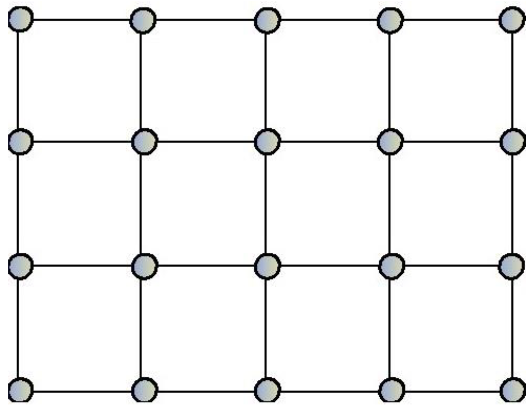
Figure 2.
2D Visualizations of Benchmark Functions.
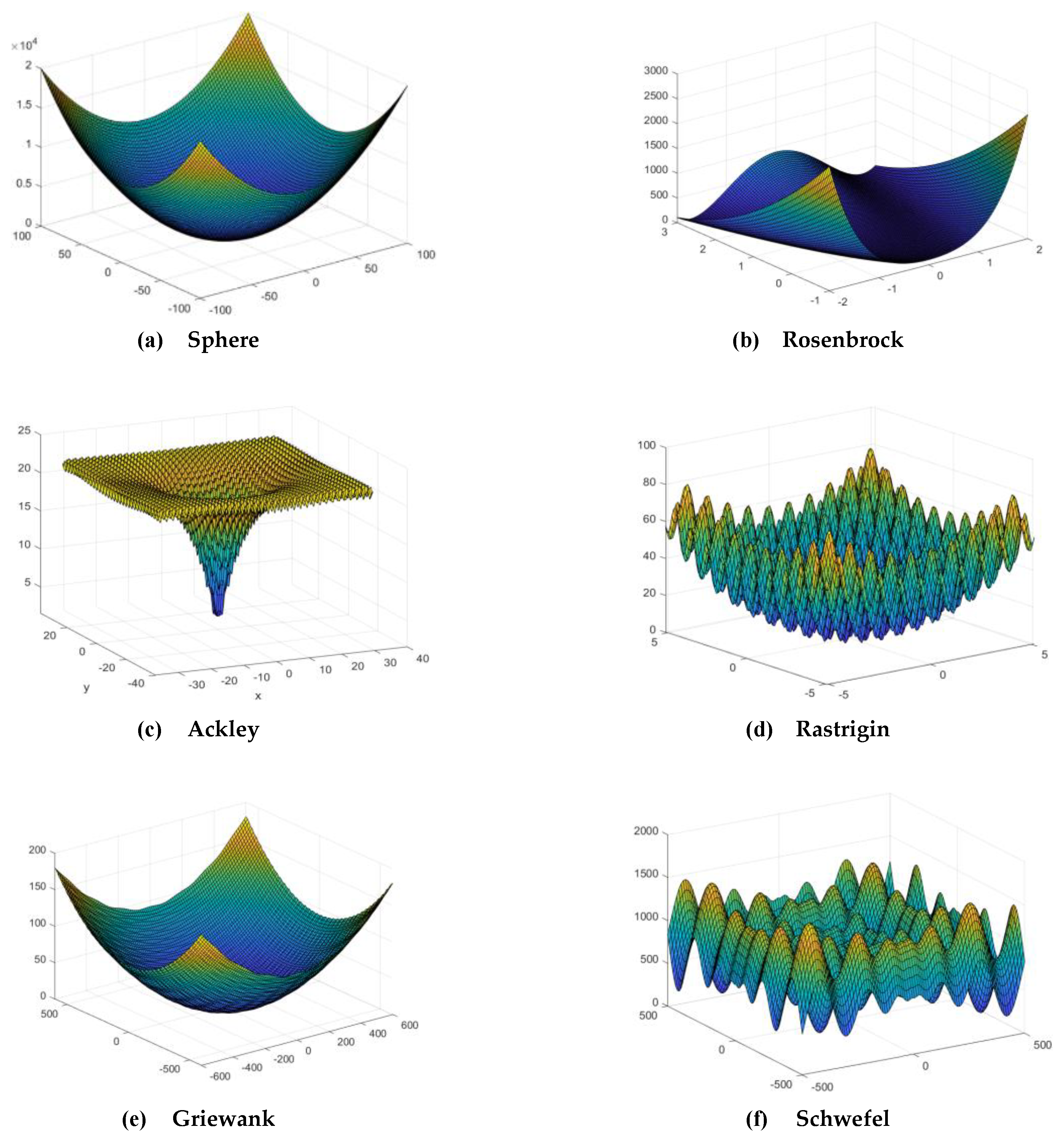
Figure 3.
The topology of a microenvironment network.
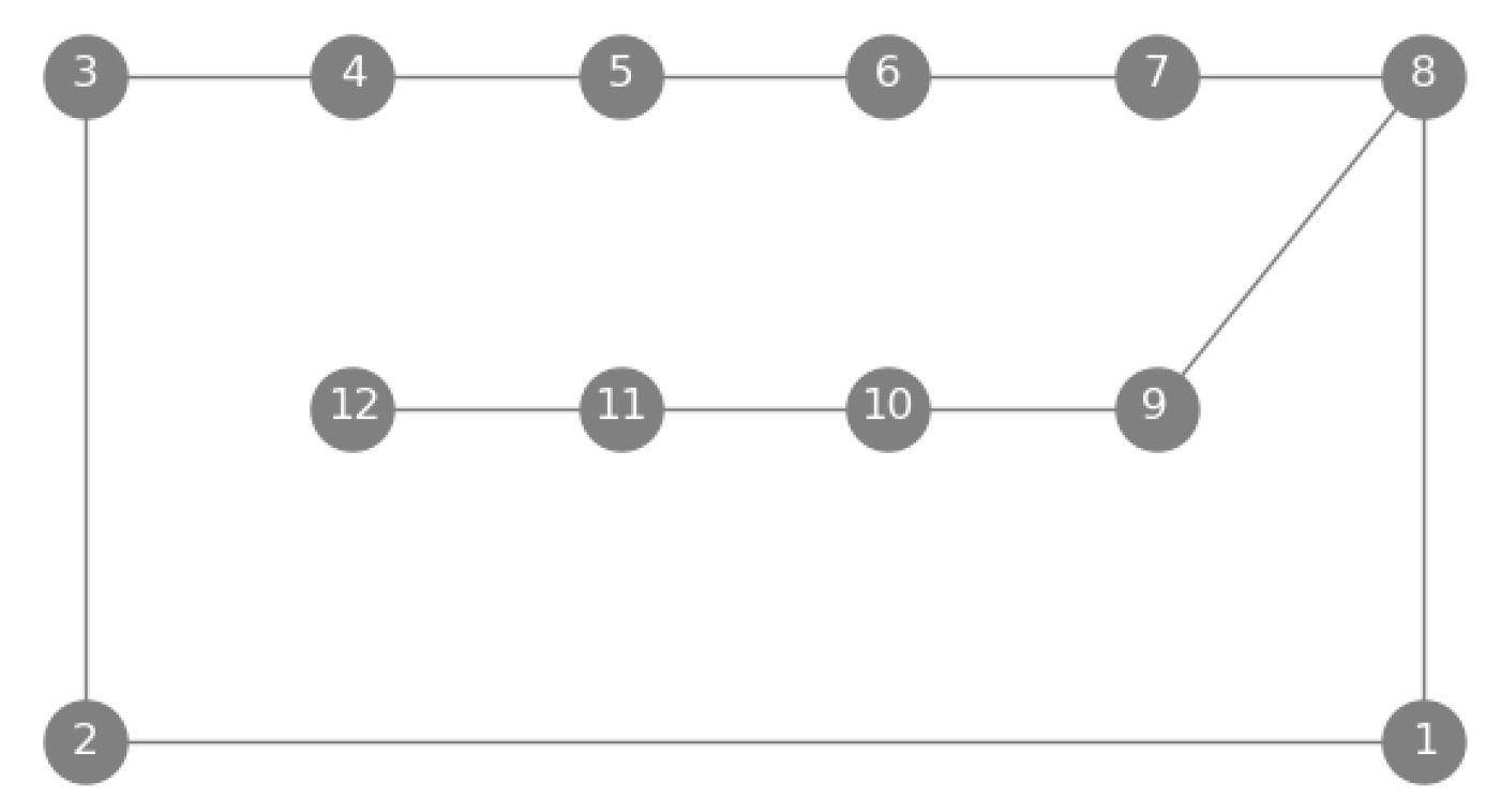
Figure 4.
The topology of 4 microenvironment networks.
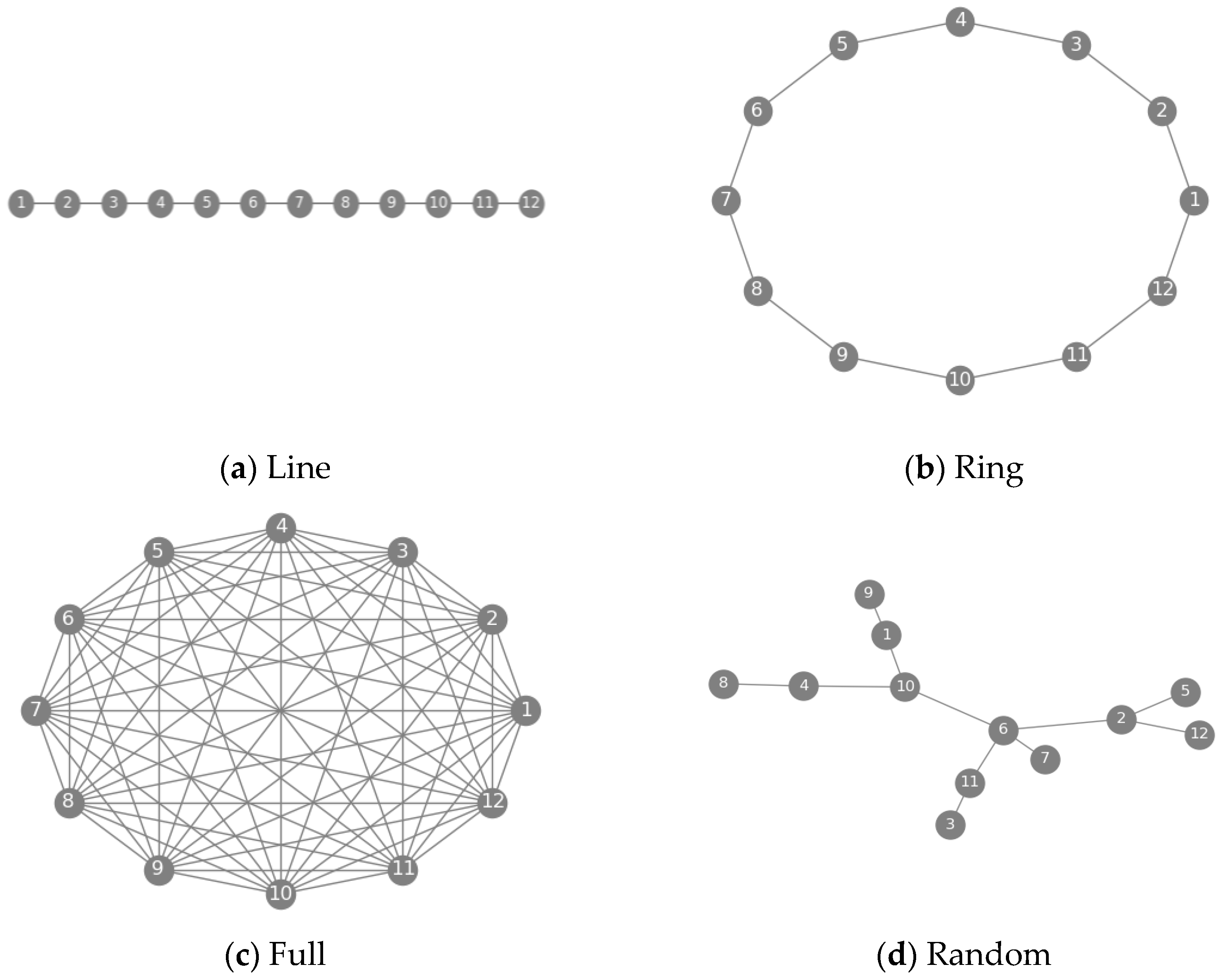
Figure 5.
Comparison of Temperature Fields Reconstructed by three PSO Algorithms.
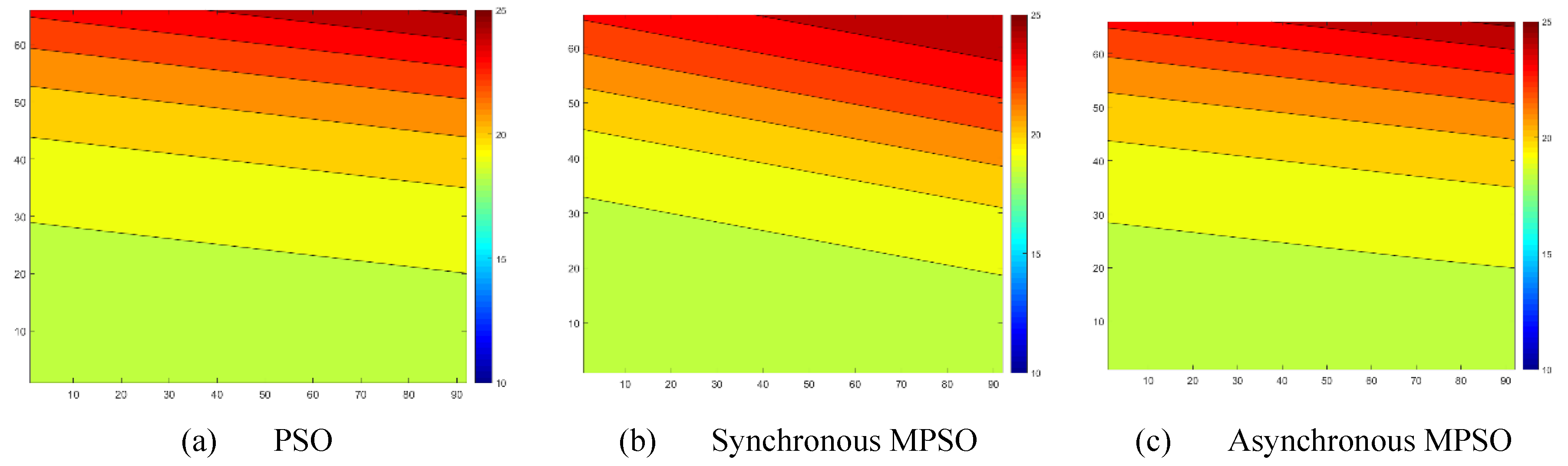

Table 1.
Benchmark functions.
| Function | Formula | Range |
|---|---|---|
| Sphere | [-100, 100] | |
| Rosenbrock | [-100, 100] | |
| Ackley | [-100, 100] | |
| Rastrigin | [-100, 100] | |
| Griewank | [-100, 100] | |
| Schwefel | [-500, 500] |
Table 2.
The performance of the PSO algorithm (maxN=200).
| Benchmark | time(second) | precision | ||||||
| minimum | maximum | mean | summary | minimum | maximum | mean | ||
| Sphere | 7 | 9 | 8.0000 | 96 | 1.4279e-11 | 2.6983e-08 | 5.7411e-09 | |
| Rosenbrock | 6 | 8 | 7.3333 | 88 | 1.6056e-09 | 3.9061e-05 | 6.5947e-06 | |
| Ackley | 8 | 10 | 9.0000 | 108 | 2.9338e-06 | 8.7710e-04 | 1.3989e-04 | |
| Rastrigin | 7 | 9 | 8.4167 | 101 | 1.2292e-12 | 8.6732e-06 | 1.4882e-06 | |
| Griewank | 7 | 9 | 8.4167 | 101 | 1.1171e-07 | 0.0074 | 0.0042 | |
| Schwefel | 7 | 9 | 7.9167 | 95 | 2.5455e-05 | 118.4384 | 11.1567 | |
Table 3.
The performance of PSO algorithm (maxN=200, goal performance=1e-5).
| Benchmark | time(second) | precision | number of iterations | ||||||
| minimum | maximum | mean | summary | minimum | maximum | mean | |||
| Sphere | 2 | 4 | 3.0000 | 36 | 1.0524e-06 | 9.9253e-06 | 4.1243e-06 | 78 | |
| Rosenbrock | 4 | 7 | 5.1667 | 62 | 1.0410e-06 | 9.0092e-05 | 1.1146e-05 | 140 | |
| Ackley | 8 | 10 | 8.7500 | 105 | 6.7112e-06 | 5.4444e-04 | 1.3135e-04 | 200 | |
| Rastrigin | 3 | 9 | 6.3333 | 76 | 4.0304e-08 | 2.1599e-05 | 7.2190e-06 | 152 | |
| Griewank | 4 | 10 | 7.3333 | 88 | 9.6462e-07 | 0.0074 | 0.0028 | 200 | |
| Schwefel* | 1 | 8 | 5.9167 | 71 | 2.6262e-05 | 25.2099 | 2.4680 | 155 | |
Table 4.
The performance of PSO algorithm (maxN=20000, goal performance=1e-5).
| Benchmark | time(second) | precision | number of iterations | ||||||
| minimum | maximum | mean | summary | minimum | maximum | mean | |||
| Sphere | 1 | 3 | 2.4167 | 29 | 8.0604e-07 | 6.5498e-06 | 3.8992e-06 | 64 | |
| Rosenbrock | 5 | 8 | 6.5000 | 78 | 7.9954e-07 | 9.9958e-06 | 5.4557e-06 | 161 | |
| Ackley | 7 | 20 | 12.5000 | 150 | 2.7555e-06 | 6.8468e-05 | 1.1611e-05 | 283 | |
| Rastrigin | 3 | 9 | 6.0833 | 73 | 1.4402e-06 | 8.0403e-06 | 4.8746e-06 | 149 | |
| Griewank | 3 | 87 | 15.9167 | 191 | 1.0553e-06 | 9.4158e-06 | 4.5158e-06 | 212 | |
| Schwefel* | 716 | 1207 | 1100.4 | 13205 | 2.5455e-05 | 335.5827 | 181.3207 | 20000 | |
Table 5.
The performance of Synchronous MPSO algorithm (maxN=200).
| Benchmark | time(second) | precision | ||||
|---|---|---|---|---|---|---|
| minimum | maximum | mean | minimum | maximum | mean | |
| Sphere | 9 | 15 | 12.0000 | 1.9026e-11 | 2.7730e-10 | 1.9970e-10 |
| Rosenbrock | 10 | 16 | 12.8333 | 2.6863e-06 | 2.6863e-06 | 2.6863e-06 |
| Ackley | 10 | 16 | 13.0000 | 5.2168e-06 | 5.2168e-06 | 5.2168e-06 |
| Rastrigin | 9 | 16 | 12.5833 | 3.0659e-08 | 3.0659e-08 | 3.0659e-08 |
| Griewank | 9 | 16 | 13.0833 | 6.6870e-07 | 1.4386e-06 | 1.0537e-06 |
| Schwefel | 14 | 15 | 14.0833 | 2.7654e-05 | 2.8024e-05 | 2.7993e-05 |
Table 6.
The performance of Synchronous MPSO algorithm (maxN=200, goal performance=1e-5).
| Benchmark | time(second) | precision | iterations | ||||
|---|---|---|---|---|---|---|---|
| minimum | maximum | mean | minimum | maximum | mean | ||
| Sphere | 2 | 15 | 9.0833 | 6.9061e-06 | 6.9061e-06 | 6.9061e-06 | 58 |
| Rosenbrock | 6 | 11 | 8.4167 | 3.5176e-06 | 3.5176e-06 | 3.5176e-06 | 135 |
| Ackley | 10 | 15 | 12.6667 | 9.2855e-06 | 9.2855e-06 | 9.2855e-06 | 183 |
| Rastrigin | 7 | 12 | 9.3333 | 3.5689e-06 | 9.9922e-06 | 4.6394e-06 | 145 |
| Griewank | 4 | 11 | 7.7500 | 1.8658e-06 | 1.8658e-06 | 1.8658e-06 | 80 |
| Schwefel* | 5 | 11 | 8.3333 | 5.0415e-05 | 5.0415e-05 | 5.0415e-05 | 132 |
Table 7.
The performance of Synchronous MPSO algorithm (maxN=20000, goal performance=1e-5).
| Benchmark | time(second) | precision | iterations | ||||
|---|---|---|---|---|---|---|---|
| minimum | maximum | mean | minimum | maximum | mean | ||
| Sphere | 3 | 11 | 6.8333 | 3.3261e-06 | 3.3261e-06 | 3.3261e-06 | 67 |
| Rosenbrock | 9 | 14 | 11.4167 | 2.3513e-06 | 2.3513e-06 | 2.3513e-06 | 173 |
| Ackley | 12 | 18 | 15.0000 | 8.9925e-06 | 9.8653e-06 | 9.6471e-06 | 243 |
| Rastrigin | 10 | 15 | 12.4167 | 1.2856e-06 | 1.2856e-06 | 1.2856e-06 | 169 |
| Griewank | 9 | 15 | 12.0000 | 3.9471e-06 | 6.3238e-06 | 6.1257e-06 | 171 |
| Schwefel* | 9 | 13 | 10.9167 | 7.3792e-05 | 7.3792e-05 | 7.3792e-05 | 196 |
Table 8.
The performance of Asynchronous MPSO algorithm (maxN=200).
| Benchmark | time(second) | precision | ||||
|---|---|---|---|---|---|---|
| minimum | maximum | minimum | maximum | minimum | maximum | |
| Sphere | 8 | 11 | 9.0000 | 1.7644e-10 | 5.2181e-08 | 1.7286e-08 |
| Rosenbrock | 7 | 12 | 8.8333 | 2.3681e-05 | 0.8435 | 0.0959 |
| Ackley | 7 | 12 | 9.2500 | 1.4856e-05 | 5.5352e-04 | 1.2233e-04 |
| Rastrigin | 8 | 13 | 9.2500 | 1.3918e-07 | 0.0171 | 0.0021 |
| Griewank | 8 | 12 | 9.3333 | 3.1917e-04 | 0.0224 | 0.0153 |
| Schwefel | 9 | 14 | 11.7500 | 1.5578e-04 | 4.2061 | 0.8016 |
Table 9.
The performance of Asynchronous MPSO algorithm (maxN=200, goal performance=1e-5).
| Benchmark | time(second) | precision | iterations | ||||
|---|---|---|---|---|---|---|---|
| minimum | maximum | mean | minimum | maximum | mean | ||
| Sphere | 3 | 7 | 5.8333 | 1.2883e-06 | 7.2896e-06 | 4.4165e-06 | 116 |
| Rosenbrock | 6 | 11 | 8.1667 | 1.4505e-06 | 0.0030 | 3.8550e-04 | 200 |
| Ackley | 7 | 13 | 8.9167 | 5.7938e-06 | 1.7202e-04 | 6.5167e-05 | 200 |
| Rastrigin | 7 | 10 | 8.2500 | 9.1335e-07 | 3.0272e-04 | 8.5521e-05 | 200 |
| Griewank | 8 | 11 | 9.0833 | 0.0074 | 0.0117 | 0.0079 | 200 |
| Schwefel* | 8 | 11 | 9.0833 | 6.7772e-05 | 2.9875 | 0.5172 | 200 |
Table 10.
The performance of Asynchronous MPSO algorithm (maxN=20000, goal performance=1e-5).
| Benchmark | time(second) | precision | iterations | ||||
|---|---|---|---|---|---|---|---|
| minimum | maximum | mean | minimum | maximum | mean | ||
| Sphere | 3 | 9 | 5.8333 | 2.1601e-07 | 8.7867e-06 | 4.7173e-06 | 127 |
| Rosenbrock | 7 | 16 | 10.4167 | 1.1558e-06 | 9.3172e-06 | 4.8171e-06 | 227 |
| Ackley | 11 | 45 | 21.6667 | 1.5834e-06 | 9.8807e-06 | 6.7718e-06 | 407 |
| Rastrigin | 7 | 22 | 10.7500 | 8.9664e-08 | 9.2383e-06 | 4.9633e-06 | 209 |
| Griewank | 11 | 69 | 26.1667 | 1.4646e-07 | 9.2350e-06 | 4.1181e-06 | 452 |
| Schwefel* | 15 | 1269 | 327.3333 | 2.8554e-05 | 2.4522e-04 | 1.0859e-04 | 520 |
Table 11.
The performance of synchronous MPSO algorithm (Line).
| Benchmark | time(second) | precision | iterations | ||||||
|---|---|---|---|---|---|---|---|---|---|
| minimum | maximum | mean | minimum | maximum | mean | minimum | maximum | median | |
| Sphere | 3 | 12 | 7.5000 | 4.2457e-07 | 4.6760e-07 | 4.4609e-07 | 76 | 85 | 81 |
| Rosenbrock | 7 | 11 | 8.4167 | 9.1477e-06 | 9.1477e-06 | 9.1477e-06 | 146 | 155 | 150 |
| Ackley | 13 | 19 | 16.2500 | 8.7556e-06 | 8.7556e-06 | 8.7556e-06 | 262 | 272 | 267 |
| Rastrigin | 7 | 10 | 8.3333 | 5.2039e-06 | 5.2039e-06 | 5.2039e-06 | 128 | 137 | 132 |
| Griewank | 38 | 42 | 40.0000 | 5.2645e-06 | 5.2645e-06 | 5.2645e-06 | 691 | 700 | 695 |
| Schwefel* | 9 | 13 | 10.3333 | 6.6853e-05 | 6.6853e-05 | 6.6853e-05 | 167 | 178 | 172.5 |
Table 12.
The performance of synchronous MPSO algorithm (Ring).
| Benchmark | time(second) | precision | iterations | ||||||
|---|---|---|---|---|---|---|---|---|---|
| minimum | maximum | mean | minimum | maximum | mean | minimum | maximum | median | |
| Sphere | 3 | 12 | 8.5833 | 5.2046e-06 | 5.2046e-06 | 5.2046e-06 | 69 | 75 | 72 |
| Rosenbrock | 8 | 13 | 10.7500 | 6.1511e-06 | 6.1511e-06 | 6.1511e-06 | 186 | 196 | 191 |
| Ackley | 14 | 17 | 15.1667 | 6.3740e-06 | 6.3740e-06 | 6.3740e-06 | 250 | 256 | 253 |
| Rastrigin | 6 | 11 | 8.2500 | 1.3716e-06 | 1.3716e-06 | 1.3716e-06 | 127 | 133 | 130 |
| Griewank | 10 | 14 | 12.5000 | 9.6413e-06 | 9.6413e-06 | 9.6413e-06 | 211 | 217 | 214 |
| Schwefel* | 9 | 14 | 11.5000 | 3.5431e-05 | 3.5431e-05 | 3.5431e-05 | 181 | 187 | 184 |
Table 13.
The performance of synchronous MPSO algorithm (Full).
| Benchmark | time(second) | precision | iterations | ||||||
|---|---|---|---|---|---|---|---|---|---|
| minimum | maximum | mean | minimum | maximum | mean | minimum | maximum | median | |
| Sphere | 5 | 11 | 8.0000 | 6.9881e-06 | 6.9881e-06 | 6.9881e-06 | 65 | 67 | 66 |
| Rosenbrock | 8 | 14 | 11.1667 | 9.9103e-06 | 9.9103e-06 | 9.9103e-06 | 119 | 120 | 120 |
| Ackley | 19 | 26 | 22.5000 | 9.9360e-06 | 9.9360e-06 | 9.9360e-06 | 267 | 268 | 268 |
| Rastrigin | 11 | 16 | 13.5833 | 4.9590e-06 | 4.9590e-06 | 4.9590e-06 | 162 | 163 | 163 |
| Griewank | 10 | 16 | 12.8333 | 1.0800e-07 | 1.0800e-07 | 1.0800e-07 | 150 | 151 | 151 |
| Schwefel* | 9 | 14 | 11.1667 | 5.4167e-05 | 5.4167e-05 | 5.4167e-05 | 125 | 127 | 126 |
Table 14.
The performance of synchronous MPSO algorithm (Random).
| Benchmark | time(second) | precision | iterations | ||||||
|---|---|---|---|---|---|---|---|---|---|
| minimum | maximum | mean | minimum | maximum | mean | minimum | maximum | median | |
| Sphere | 3 | 8 | 5.5000 | 1.0932e-06 | 1.0932e-06 | 1.0932e-06 | 67 | 71 | 70 |
| Rosenbrock | 6 | 10 | 8.2500 | 7.6528e-06 | 7.6528e-06 | 7.6528e-06 | 134 | 139 | 137 |
| Ackley | 9 | 15 | 11.8333 | 9.4930e-06 | 9.4968e-06 | 9.4958e-06 | 182 | 186 | 185 |
| Rastrigin | 7 | 11 | 8.9167 | 3.5646e-06 | 3.5646e-06 | 3.5646e-06 | 125 | 129 | 127 |
| Griewank | 9 | 14 | 11.0000 | 1.0142e-06 | 1.0142e-06 | 1.0142e-06 | 180 | 183 | 182 |
| Schwefel* | 7 | 20 | 15.4167 | 9.5925e-05 | 9.5925e-05 | 9.5925e-05 | 153 | 158 | 156 |
Table 15.
Performance comparison of PSO and MPSO for temperature field reconstruction.
| Algorithm | time(second) | precision | iterations | ||||||
|---|---|---|---|---|---|---|---|---|---|
| min | max | mean | min | max | mean | min | max | median | |
| PSO | 69 | 181 | 166.4167 | 3.0331e-09 | 1.3406 | 0.3263 | 991 | 2000 | 2000 |
| Synchronous MPSO | 83 | 84 | 83.9167 | 9.5743e-09 | 9.5743e-09 | 9.5743e-09 | 787 | 792 | 790 |
| Asynchronous MPSO | 45 | 151 | 74.1667 | 4.4517e-09 | 9.9995e-09 | 8.1274e-09 | 545 | 1829 | 678 |
Disclaimer/Publisher’s Note: The statements, opinions and data contained in all publications are solely those of the individual author(s) and contributor(s) and not of MDPI and/or the editor(s). MDPI and/or the editor(s) disclaim responsibility for any injury to people or property resulting from any ideas, methods, instructions or products referred to in the content. |
© 2025 by the authors. Licensee MDPI, Basel, Switzerland. This article is an open access article distributed under the terms and conditions of the Creative Commons Attribution (CC BY) license (http://creativecommons.org/licenses/by/4.0/).
Copyright: This open access article is published under a Creative Commons CC BY 4.0 license, which permit the free download, distribution, and reuse, provided that the author and preprint are cited in any reuse.