Submitted:
27 March 2025
Posted:
27 March 2025
You are already at the latest version
Abstract
In the increasingly complex electromagnetic environment, accurately recognizing unknown types of active radar jamming signals has become a task of significant research importance and considerable challenge. Most current intelligent jamming recognition methods struggle to effectively handle unknown jamming signals. Although some open-set jamming recognition algorithms have achieved a certain level of discrimination for unknown jamming in recent years, the introduction of unknown jamming often severely impacts their closed-set recognition performance, especially under low Jamming-to-Noise Ratio(JNR) conditions, where the overall model performance significantly declines. To address these issues, this paper proposes an Open-Set Recognition(OSR) optimization method based on multi-dimensional prototype feature constraints and adversarial reciprocal point learning, termed MDPAR, aiming to simultaneously improve the rejection capability for unknown jamming signals and the closed-set classification accuracy for known jamming signals. First, based on prototype points, a Multi-Dimensional Prototype Feature Constraint(MDPFC) is proposed. By designing Intra-class Compactness Loss(ICL), Inter-class Boundary Loss(IBL), and open-point cosine loss, we optimized the distribution of the feature space for known classes. Second, we introduced an Adversarial margin-based Reciprocal Point Learning method(ARPL) to model the open space where unknown jamming signals reside. Additionally, an Associated Soft Constraint(ASC) between open points and reciprocal points is proposed to jointly optimize and unify the overall distribution of the open space. Finally, the jamming signal data, after domain transformation, is input into the feature extraction network, and the MDPAR model is used for training and testing. Experimental results demonstrate that the proposed MDPAR method exhibits excellent performance across multiple OSR evaluation metrics. Particularly, under conditions where the Jamming-to-Signal Ratio(JSR) is 5 dB and the Signal-to-Noise Ratio(SNR) is above 0 dB, the recognition rate for unknown jamming signals remains above 90\%. Furthermore, through threshold visualization and t-SNE dimensionality reduction analysis of the MDPAR prediction results, clear boundaries between unknown and known class samples are formed, and significant inter-class separation structures are observed within known classes, further validating the effectiveness and advancement of MDPAR in the task of OSR for radar jamming signals.
Keywords:
radar active jamming
; open-set recognition
; neural networks
; multi-dimensional prototype feature constraint
; adversarial reciprocal point learning
1. Introduction
In the complex and dynamic modern electromagnetic environment, radar systems are confronted with a myriad of threats from active jamming signals, posing significant challenges to the anti-jamming strategies of radar systems [1]. With the increasing sophistication of Digital Radio Frequency Memory(DRFM)technology, the variety of new active jamming signals continues to expand, and the styles of jamming become increasingly complex. For radar systems to maintain normal operation, it is imperative to accurately identify the types of active jamming in order to promptly adopt effective countermeasures [2]. As electronic warfare gradually evolves from traditional methods to intelligent approaches, the recognition of active radar jamming, being a crucial component of intelligent radar counter-jamming, is of paramount importance to the field [3]. Therefore, conducting research on more intelligent recognition of active radar jamming signals holds significant theoretical and practical implications.
In recent years, with the continuous advancement of machine learning and deep learning, their formidable capabilities in processing complex data have led to widespread applications across various domains [4]. Numerous experts and scholars have leveraged machine learning and deep learning methodologies to conduct extensive work in the field of intelligent radar jamming recognition, yielding a plethora of research outcomes. The recognition of active radar jamming based on machine learning necessitates the integration of feature engineering to achieve the goal of intelligence. Su et al. [5] extracted a set of feature parameters from radar jamming signals that exhibit low sensitivity to noise, low computational complexity, and minimal influence from jamming parameters, utilizing these for jamming recognition and achieving commendable recognition performance on typical radar jamming patterns. Xu et al. [6] derived a set of highly separable features from the time domain, frequency domain, and Time-Frequency domain, which were then fed into decision trees and Support Vector Machines(SVM) for jamming recognition, effectively identifying seven typical types of suppression and deception jamming. Zhou et al. [7] enhanced the algorithm using bispectrum transformation and kernel density estimation, using a feature fusion algorithm based on Bayesian decision theory to recognize radar received signals, a method that proficiently identifies radar deceptive jamming. The recognition of active radar jamming based on deep learning is more intelligent, capable of adaptively filtering and representing data features across multiple domains of the signal, with recognition performance that exhibits stronger generalization and robustness. In reference [8], the Zernike moments were calculated from the Smoothed Pseudo Wigner-Ville Distribution(SPWD) of the jamming signals and used as feature vectors for signal recognition input into a Convolutional Neural Network(CNN), achieving considerable recognition effectiveness. Wang et al. [9] proposed a novel Siamese network architecture with self-attention capabilities, SA-Siam, which transforms jamming signals into the Time-Frequency(TF) domain. The Siamese network, in conjunction with the Self-Attention block(SA), further distinguishes radar jamming signals and captures the spatial correlations of TF images. The results indicate that this method can achieve commendable jamming recognition performance even with a limited number of jamming signal samples. Reference [10] introduced a novel Jamming Recognition Network(JRNet) based on robust power spectrum features by integrating residual blocks and asymmetric convolutional blocks. JRNet is capable of addressing the degradation problem and enhancing the recognition capability of subtle features. Experimental results on ten types of jamming signals demonstrate that JRNet achieves superior and more stable recognition performance, with an overall recognition accuracy exceeding 90% even at a Jamming-to-Noise Ratio(JNR) of −18 dB. Wei and his team [11], targeting scenarios with limited data, proposed a rapid active jamming recognition method based on a hybrid CNN-Transformer model. This method extracts local features from the complex domain, real part, and imaginary part of the jamming signals through three CNNs, concatenates these features, and then applies positional encoding, followed by the use of Transformer to capture global features. The experimental results indicate that this method not only effectively improves training speed and recognition accuracy but also enables fast and reliable recognition of jamming signals in resource-constrained environments.
However, existing intelligent radar jamming recognition typically assumes that the jamming categories during both training and testing phases are fully known, i.e., the closed-set assumption. In practical applications, the electromagnetic environment faced by radar is complex and variable, with the types of jamming signals being highly uncertain and open, and there exists a vast array of unknown jamming signals [12]. Traditional recognition methods under the closed-set assumption are unable to effectively detect these unknown categories, often misclassifying unknown jamming as known categories, leading to a sharp decline in system performance [13,14]. Therefore, in an open world, Open-Set Recognition(OSR) is gradually becoming an important research direction in the field of radar signal processing.
Currently, with the increasing complexity of electronic countermeasure technologies and the growing demand for radar systems to recognize unknown jamming signals, more and more scholars are beginning to focus on this field and gradually conducting related research. Li et al. [15] proposed a pseudo-label CNN model based on generative adversarial networks, which takes the Time-Frequency features of radar jamming signals as input and intelligently increases labeled samples using adaptive pseudo-labeling methods and generative adversarial networks to achieve semi-supervised recognition of radar jamming, with recognition rates for unknown types ranging from 30.7% to 86.8%. In reference [12], Han proposed an unsupervised jamming pattern recognition scheme based on Zero-Shot Learning(ZSL), and the proposed scheme achieved excellent performance in handling open-set tasks. Reference [16] introduced a multi-task multi-label open-set composite jamming signal recognition framework, which utilizes the time-frequency characteristics of composite jamming signals for multi-label classification while integrating unknown signal detection into the classification process. This method exhibits high recognition accuracy in closed-set environments and strong detection capabilities for unknown signals in open-set environments, effectively enhancing the reliability of jamming systems. Zhou et al. [17] proposed two radar jamming OSR models based on confidence scores and OpenMax, which demonstrate high recognition accuracy for both known and unknown jamming under small sample conditions by outputting the probabilities of jamming belonging to all known classes and the probability of jamming belonging to unknown classes, thereby improving the perception capabilities in complex jamming environments. Reference [18] studied an OSR method for active jamming signals based on relative entropy, using the relative entropy between recognition probability and ideal probability as confidence, and achieving OSR through a voting mechanism on recognition probability and relative entropy, with recognition probabilities exceeding 90% when the JNR is above 10dB. Zhang et al. [19] proposed the RCAE-OWR method, incorporating center loss and reconstruction loss into the Softmax loss to optimize intra-class and inter-class distributions, and the experimental results show that when the JNR exceeds 10 dB, the recognition rate surpasses 92%, which could validate that the method could effectively identify both known and unknown interference.
Despite of existing research has made some progress in the field of OSR for radar jamming signals, most intelligent recognition methods still struggle to effectively handle unknown jamming signals. While some OSR algorithms have achieved a certain level of capability to reject unknown jamming, the introduction of unknown class jamming often significantly impacts their closed-set recognition performance, especially under low JNR conditions, where the overall model performance noticeably declines. To address this issue, this paper proposes an OSR optimization method based on multi-dimensional prototype feature constraints and adversarial reciprocal point learning, termed MDPAR, aiming to effectively enhance the rejection capability for unknown jamming signals while maintaining high closed-set recognition performance for known jamming signals. From the start, we proposed a Multi-Dimensional Prototype Feature Constraint(MDPFC) based on prototype points. By designing Intra-class Compactness Loss(ICL), Inter-class Boundary Loss(IBL), and open-point cosine loss, the distribution of the feature space for known classes is jointly optimized. Next step, we introduced an Adversarial margin-based Reciprocal Point Learning(ARPL) method in order to explicitly model the open space where unknown jamming signals reside. Furthermore, an Associated Soft Constraint(ASC) between open points and reciprocal points is proposed to jointly optimize and unify the overall representation of unknown classes in the feature space. Finally, the jamming signal data, after domain transformation, is input into the feature extraction network, and the MDPAR model is used for training and testing. Experimental results demonstrate that MDPAR exhibits excellent performance across multiple OSR evaluation metrics. Through threshold visualization and t-SNE dimensionality reduction analysis, clear boundaries between unknown and known classes are formed, and significant inter-class separation structures are observed within known classes, fully validating the effectiveness and advancement of MDPAR in the task of OSR for radar jamming signals. Additionally, this study further designs comparative experiments for OSR methods and ablation experiments for the components of MDPAR, thoroughly exploring and verifying the effectiveness and contributions of each module in the MDPAR method.
2. Modeling and Processing of Active Radar Jamming Signals
2.1. Modeling of Active Radar Jamming Signals
Radar jamming encompasses a wide variety of types, we could simply classify them into active jamming and passive jamming based on the energy source of the jamming signals. Active jamming refers to the use of electromagnetic wave energy for interference, and it can be broadly categorized into suppression jamming and deception jamming [20]. Suppression jamming overloads the receiving equipment by increasing signal energy, while deception jamming interferes with enemy recognition by altering signal parameters to create false targets or mislead target positions [21]. This section primarily focuses on the modeling of active jamming signals and elaborates on the preprocessing methods used in this paper for jamming signals, aiming to provide a reliable foundation of data and feature representation for subsequent jamming signal recognition.
In radar jamming and anti-jamming training, the signals received by the radar receiver include radar echo signals, jamming signals, and noise signals, which can be expressed by the following equation.
The typical modulation types of radar signals include Continuous Wave(CW), Linear Frequency Modulation(LFM), Phase Shift Keying(PSK), and Frequency Shift Keying(FSK). Among these, LFM is the most widely used, with its frequency changing linearly over time, characterized by a large bandwidth and long pulse, which can effectively balance the radar’s range and range resolution [22]. Therefore, this paper selects the LFM signal as the radar transmission signal for this research, and its expression is given by the following equation [23].
In Equation (1), the signal frequency could be expressed as , represents the starting frequency of the signal. represents the rate of change slope, A represents the signal amplitude, represents the rectangular pulse with the width of T.
This paper uses the LFM signal as the transmitted signal and selects 11 typical active radar jamming methods as our research subjects, which include: Amplitude Modulation Jamming(AM), Comb Jamming(CJ), Frequency Modulation Jamming(FM), Interrupted Sampling Repeater Jamming (ISRJ), Multiplicative Noise Jamming(MNJ), Smeared Spectrum Jamming(SMSP), Range Gate Pull-Off Jamming(RGPO), Velocity Gate Pull-Off Jamming(VGPO), Range-Velocity Gate Pull-Off Jamming(R-VGPO), Range Multi-False-Target Jamming(RMT), and Velocity Multi-false-target Jamming(VMT).
2.2. Time-Frequency Transform Preprocessing
To obtain the time-frequency domain data of the jamming signals, it is essential to select an appropriate time-frequency transformation method. This research uses the Short-Time Fourier Transform(STFT) [24] for time-frequency analysis. Compared to the WVD [25], STFT not only effectively avoids cross-term interference but also has lower computational complexity and excellent noise robustness [26], thereby providing a solid foundation for subsequent feature extraction and classification tasks. Therefore, we use STFT to acquire the time-frequency distribution of the jamming signals and scales the image size to a predetermined pixels. These time-frequency images serve as model inputs, capturing both the global time-frequency domain characteristics of the signal and preserving local details. For the echo signal mixed with jamming signals and noise, its Fourier transform expression is as follows.
In which, represents the window function, represents the kernel function of the Fourier transform
Under the condition of a signal-to-noise ratio of 0 dB, we randomly sampled the time-frequency distribution images of 11 types of active jamming signals, and the results are shown in Figure 1.
3. Open-Set Recognition Task Modeling for Jamming Signals
This section introduces and analyzes the Open-Set Recognition(OSR) problem for active radar jamming signals. In contrast to traditional closed-set recognition tasks, where training and test sets share identical categories, OSR tasks involve test signals from unknown categories. Thus, recognition models must not only accurately classify known jamming signals but also effectively identify and reject unknown signals [27]. Since unknown signal categories are absent during training, traditional closed-set methods cannot reliably distinguish unknown signals from known ones, presenting the primary challenge in OSR tasks.
As shown in Figure 2, although known class features have been separated clearly in the closed-set feature space, unknown class features remain intermixed and scattered among known classes, often causing misclassification into the nearest known class. To achieve OSR, it is necessary to effectively separate unknown class features from known classes using threshold-based discrimination. Figure 2 also illustrates an open-set feature space, where unknown-class features are clearly distinguished from those of known classes.
In the feature space mapped by radar jamming signals, besides the space occupied by known classes, unknown-class signals reside within the so-called open space O. Samples in this open space carry the risk of being misclassified as known classes, termed open space risk . Letting denote the entire feature space, the mathematical definition of open space risk is expressed as follows [28].
Here, f denotes the classifier function mapping input sample x into binary outputs: =1 indicates recognition as a known class, while =0 denotes an unknown class or rejection from known classes. As illustrated by Equation (3), more samples incorrectly identified as known classes correspond to higher open space risk.
In radar jamming OSR tasks, the goal is to find a classifier f that maximizes accuracy, accurately classifying known signals while effectively detecting unknown signals. Thus, the empirical classification risk for known classes and the open space risk for unknown classes must both be considered. The optimization objective for OSR tasks is defined in Equation (4), where f is iteratively optimized by minimizing .
In Equation (4), H represents the Hilbert space, is the regularization coefficient, and V is the training sample dataset.
Next, we further analyze the OSR task for radar jamming signals. The training dataset can be constructed directly from an existing known jamming library. Assuming there are N labeled samples belonging to K known classes, the radar jamming training dataset is defined in Equation (5).
In Equation (5), and denote the jamming signal sample and its corresponding class label, respectively, where . The test set includes signals from both known and unknown classes. Assuming the test set contains M samples, it can be expressed as Equation (6).
In Equation (6), denotes the signal sample data with labels from the set , where U indicates the number of unknown classes. The feature space mapped from signals of class l after feature extraction is defined as , and its open space is denoted as . can be further divided into occupied by other known classes, and occupied by unknown classes. Thus, the global feature space for class l can be defined as follows.
For class l, the core of the OSR task lies in continuously optimizing and finding a binary classification function to minimize the overall risk . The optimization objective can be written as follows.
In Equation (8), is a regularization coefficient constant used to allocate the weight of .
For K different classes of signals, the problem transforms from a binary classification problem to an open-set multi-class classification problem. The optimization objective becomes:
In Equation (9), f represents the multi-class classification network model, and its optimization objective is essentially consistent with Equation (4). Equation (9) provides a more intuitive representation of the optimization objective, with the ultimate goal of finding a classification network that minimizes the sum of the empirical risk for known class radar jamming classification and the open space risk for unknown class jamming.
4. Proposed OSR Method
This section will provide a detailed exposition of the OSR method proposed in this paper, with a focus on its theoretical principles and key technologies. This includes the design of the feature extraction network, the implementation of multi-dimensional prototype feature constraints, the analysis of the adversarial reciprocal point optimization strategy, and the algorithm based on multi-dimensional prototype feature constraints and adversarial reciprocal point learning. The aim is to comprehensively analyze how the proposed method ensures excellent closed-set performance and effectively resolves the boundary ambiguity between known and unknown classes to enhance OSR performance.
4.1. Feature Extraction Neural Network
We have designed a feature extraction network specifically for the OSR task of radar jamming, which takes the time-frequency diagrams of radar jamming signals as input and maps them to high-dimensional feature vectors to support subsequent classifier tasks for known class classification and unknown class detection. The Convolutional Neural Network(CNN) used in this paper has a hierarchical structure capable of extracting robust and discriminative features from the input data, and its overall architecture is shown in Figure 3.
The network consists of multiple convolutional modules, each composed of several convolutional layers, designed to extract features at different levels of abstraction. The input to this feature extraction network is a radar jamming time-frequency diagram of size , and the entire network is made up of several convolutional modules, each containing three layers of convolutional operations that extract features and progressively compress the spatial dimensions of the feature maps. Specifically, the first two layers of each module have convolutional kernels of size , a stride of 1, and padding of 1, primarily extracting local detailed features; the third layer also has a convolutional kernel size of , but the stride is adjusted to 2 with padding of 1, effectively reducing the spatial dimensions of the feature maps through downsampling while aggregating local feature information. The number of output channels for the convolutional modules gradually increases with depth, starting from 64 in the first module and progressively increasing to 128 and 512, enhancing the feature representation capability.
To improve the model’s generalization ability and training stability, Batch Normalization(BN) and the Leaky ReLU activation function are added after each convolutional operation; the former accelerates convergence, while the latter enhances nonlinear expression. Additionally, a Dropout layer is introduced before the first layer of each convolutional module with a Dropout rate set to to mitigate the risk of overfitting. By randomly suppressing the activation of some neurons, the model’s excessive reliance on training data is reduced, thereby enhancing the model’s robustness to unknown samples.
After passing through all convolutional modules, the size of the feature map output by the network is . To extract global features and reduce computational complexity, the network includes a Global Average Pooling(GAP) layer after the convolutional modules, compressing the feature map into a 512-dimensional vector. This vector integrates global and local information, possesses high discriminative power, and is mapped to a probability distribution of categories through a fully connected layer and Softmax activation function, used for known class classification and unknown class detection.
The feature extraction network in this paper enhances robustness and generalization ability through regularization techniques such as Dropout, BN and Leaky ReLU.
4.2. Multi-Dimensional Prototype Feature Constraint
In the task of OSR for radar jamming, the distribution of known and unknown classes in the feature space is quite complex. Optimizing the distribution of known class features is key to improving classification performance [29]. To address this issue, we propose a multi-dimensional prototype feature constraint optimization method that comprehensively optimizes the feature distribution of known classes from two dimensions: intra-class compactness and inter-class separation. Additionally, based on the concept of prototype points, we introduce the notion of open points [30] to initially model the open space where unknown classes reside, providing reasonable constraints and optimization for the boundary between unknown and known classes, while further optimizing the distribution of known class features, thereby effectively enhancing the model’s overall performance in OSR tasks. Next, we will elaborate on and analyze the relevant technical principles and specific implementation methods.
4.2.1. Intra-class and Inter-class Prototype Feature Constraint Optimization
Intra-class compactness is an important part of optimizing the feature distribution of known classes, aiming to make the features of samples within the same category more concentrated, thereby reducing intra-class variance. To achieve this goal, this paper introduces prototype points as the feature centers of known categories in the feature space. It is important to note that in this study, each known class has a unique prototype point to avoid the increased risk of open space that multiple prototype points might cause. The prototype point can be represented by the following Equation (10).
In Equation (10), and represent the prototype point for signals of class l and the number of samples belonging to that class, respectively. represents the feature vector of the i-th sample belonging to that class, and K is the number of known classes.
During the optimization process, to make the sample features closer to the prototype points of their corresponding classes, this paper designs a distance-based loss function. The goal is to minimize the Euclidean distance between the samples and the prototype points, . Here, represents the Euclidean distance between sample and the prototype point of its corresponding class l. By normalizing the Euclidean distance using Softmax and then applying cross-entropy loss to enable the model to better classify known features, the Intra-class Compactness Loss(ICL) is obtained, as shown in the following equation.
Optimizing only intra-class compactness may lead to overlapping feature distributions of different classes, thereby reducing the model’s discriminative ability. To address this, this paper further introduces inter-class separation constraints and constructs a Generalized Margin Classification Loss(GMCL) [31]. By enhancing the minimum margin between prototype points of different classes, the class boundaries in the feature space are optimized.
For the sample feature , in addition to calculating its distance to the prototype point of its corresponding class l, , an additional constraint is applied to its minimum Euclidean distance to the prototype points of other known classes, . By comparing the relative difference between and , and incorporating the margin hyperparameter, the Inter-Boundary Loss(IBL) is designed as follows.
Figure 4 illustrates the distribution structure of known class samples in the feature space under the joint optimization of ICL and IBL. Through the constraints of ICL, samples of the same class cluster toward their respective prototype centers, forming compact intra-class distributions. At the same time, IBL enhances the boundary distances between class prototype points, significantly improving inter-class discriminability. This optimization ensures both intra-class compactness and effectively avoids overlapping feature distributions between classes, providing the classifier with a more stable and clear feature space structure, thereby reducing the empirical risk caused by classification.
4.2.2. Prototype Open Point Constraint Optimization
Simply optimizing the distribution of known class features cannot directly handle unknown class jamming samples. We also need to reasonably model the distribution of unknown class samples to reduce the risk of unknown samples being misclassified as known classes. To this end, this paper introduces the concept of open points based on prototype learning to explicitly model the potential distribution regions of unknown classes in the feature space, thereby providing reasonable feature representations for unknown classes.
The open point is the mean of the prototype points of all known classes, which, in a sense, can be used to represent the inherent feature center of unknown classes. It can preliminarily model the potential distribution regions of unknown classes in the feature space. The mathematical definition of the open point is as follows.
Open point learning allows the spatial distribution of unknown class samples to contract to some extent, attracting unknown class samples and repelling them from known class samples, thereby reducing open space risk. A schematic diagram of this process is shown in Figure 5. To achieve this goal, a cosine similarity constraint mechanism is used to optimize the functionality of the open point. By limiting the cosine similarity between unknown class samples, known class prototype points, and the open point, the distribution relationships in the feature space can be more precisely adjusted, thereby better achieving the goals of repulsion and attraction of the open point. The vector between the sample feature and its corresponding class prototype point is defined as , and the vector between the prototype point and the open point is defined as . The specific mathematical expressions are given in Equation (14).
The goal of the cosine similarity constraint mechanism is to maximize the cosine value of the angle between vectors and . To facilitate subsequent mathematical expressions and avoid conflicts during the optimization of the loss function, the cosine similarity constraint loss is defined as follows.
By minimizing , the model can, to some extent, attract unknown class samples to the vicinity of the open point while avoiding conflicts with known class prototype points. Additionally, it can further compress the intra-class distribution space of known classes.
To comprehensively optimize the distribution of the feature space, this paper jointly designs ICL, IBL, and the open point cosine constraint loss to construct the complete multi-dimensional prototype feature constraint optimization objective function , as shown in Equation (16).
In Equation (16), is the regularization coefficient for the inter-class boundary loss of known classes, used to balance the degree of inter-class separation. Specifically, ICL is used to enhance the intra-class compactness of known class samples, making the sample features more concentrated around their corresponding prototype points. IBL ensures clear decision boundaries between different classes in the feature space by optimizing inter-class separation. The introduction of the open point-based cosine constraint further compresses the intra-class distribution while preliminarily modeling the distribution regions of unknown classes, forming a fuzzy boundary between unknown and known classes.
4.3. Adversarial Reciprocal Points Learning
Due to the complexity of unknown class distributions and the uncertainty of open regions in feature space, relying solely on the MDPFC method for ambiguous boundary delineation is insufficient to effectively distinguish between known and unknown classes. To further clarify the decision boundary between known and unknown classes, we choose to use Adversarial Reciprocal Point Learning(ARPL) [32] to achieve this objective.
4.3.1. Reciprocal Point Definition
Reciprocal points can essentially be regarded as the opposite of prototype points. While prototype points are used to represent the central features of a known class, the reciprocal point for each class is used to represent the opposite center of its external feature space [33]. The specific distribution of the feature space is illustrated in Figure 6.
The reciprocal point for class l is defined as , which represents the samples in the open space , including . Here, represents the sample data of class l, represents the known class samples that do not belong to class l, and represents the unknown class samples. ARPL maximizes the distance between known class samples and their corresponding reciprocal points to achieve separation between the known class space and the unknown class space. Furthermore, through an adversarial margin optimization mechanism, adversarial learning is performed between reciprocal points and known class samples, effectively forming the boundary between the intra-class sample embedding space and the open space of external samples, thereby minimizing the overlapping region between known and unknown distributions. In short, for samples of class l, the distance from all samples in to should be less than the distance from samples in to . The optimization objective can be expressed as Equation (17).
In Equation (17), represents the set of pairwise distances between all samples in two sample sets in the feature space. In ARPL, the distance metric is a linear combination of the Euclidean distance and the vector dot product. Introducing the vector dot product allows for a better evaluation of the similarity between the embedded features and the reciprocal point. For an input sample x, the mathematical expression of the distance metric is as follows.
In Equation (18), represents the feature extraction network function, which maps low-dimensional samples to a high-dimensional feature space, and m is the dimensionality of the feature space.
4.3.2. Reducing Empirical Classification Risk
To minimize the overlap between samples in and for more effective distinction, a bounded distance threshold R is used to limit the spatial extent of , thereby reducing the open space risk . This is achieved by ensuring that the distance between samples in and does not exceed R, as expressed mathematically in Equation (19).
For samples x whose distance exceeds R, their distance to the reciprocal points of each class is calculated according to Equation (18) to determine their category. The probability that x belongs to class l is normalized by the Softmax function, as shown in Equation (20).
The probability that sample x is classified as class l is proportional to the distance between the feature and . Therefore, the loss function for reciprocal point classification can be expressed as below.
4.3.3. Reducing Open Space Risk
When identifying and classifying signal samples of unknown classes, the optimization objective function is Equation (17). However, since does not appear during the model’s training phase and only comes from the open environment during the testing phase, it is impossible to reduce by limiting through Equation (17). Considering that and are complementary to each other, the spatial extent of the open space can be indirectly constrained by ensuring that the distance between samples in and is greater than R. The open space loss function can be defined by Equation (22).
Simultaneously minimizing and is equivalent to ensuring that is as small as possible relative to the bounded distance threshold R, where R is also continuously learned and updated during the optimization process. The overall final loss function can be expressed as a linear combination of and , as shown below.
In Equation (23), represents the regularization coefficient for the open space loss, used to control the weight allocation of open space risk during the optimization process. Optimizing aims to increase the distance between and , thereby enhancing the model’s ability to classify known classes based on distance. At the same time, optimizing during the process of optimizing ensures that , as an external sample of , is constrained by , limiting it to a spatial range where its distance to does not exceed R. This constraint mechanism promotes mutual constraints among known class samples and continuously adjusts their distribution through adversarial training. During this process, the adversarial optimization between known class samples and reciprocal points gradually pushes known classes toward the edges of the feature space, while unknown class samples are pushed toward the center, as shown in Figure 7. Therefore, this paper defines as the Against Margin Constraint(AMC) loss. By optimizing , a significantly different distribution pattern between known and unknown classes can be formed in the feature space, enabling the model to more effectively distinguish unknown class samples based on distance.
4.4. Multi-Dimensional Prototype and Adversarial Reciprocal Learning Method
In the complex and dynamic OSR scenarios of active radar jamming signals, it is necessary to simultaneously ensure the accurate recognition of known classes and the effective detection of unknown classes. To this end, the previous sections introduced MDPFC and ARPL, which are dedicated to optimizing the feature distribution of known classes and repelling unknown classes, respectively. However, when used independently, these methods often struggle to balance high closed-set accuracy with low open-space risk within the same model. Based on the above analysis, this paper proposes a Multi-Dimensional Prototype and Adversarial Reciprocal Learning method(MDPAR) to address the radar jamming OSR problem. Furthermore, the concept of "open points as the centroid of reciprocal points with relaxation" is introduced to flexibly and uniformly model the distribution centers of unknown classes in feature space, thereby effectively enhancing the model’s detection capability for unknown classes. The principle and feature space learning process of MDPAR are illustrated in Figure 8.
Specifically, MDPFC and ARPL optimize the feature space from different perspectives. While the open points in MDPFC and the reciprocal points in ARPL can both model and represent the open space to varying degrees, they lack an organic connection between them. This may lead to a multi-centered and fragmented distribution of unknown classes in the feature space, which is not conducive to globally consistent discrimination. To address this, we introduce an Associated Soft Constraint(ASC) strategy on the basis of linearly combining MDPFC and ARPL. This strategy aims to maintain a closer global connection between open points and reciprocal points while not interfering with the adversarial repulsion mechanism’s characterization of the differentiated features of each known class. Referring to Figure 8, we aim to globally treat unknown classes as a "central anchor point," and thus consider approximating the open point as the weighted average of all reciprocal points, applying a soft constraint in the form of an arithmetic mean. For this purpose, we define the associated soft constraint loss as shown in Equation (24).
If the deviation between and is too large, the model will incur additional penalties during training, continuously pulling them toward the weighted center. If some reciprocal points maintain a certain deviation due to the unique distribution of a specific external class, the model can balance this difference using AMC without being forced to completely overlap with the open point. ASC ensures both the global convergence of unknown representations and the local dispersion of reciprocal points, thereby balancing the centralized concept of unknown classes and the differentiated repulsion of external distributions of different known classes.
The overall loss of MDPAR can be expressed as follows.
In Equation (25), is a hyperparameter that balances the contributions of MDPFC and ARPL in the overall optimization process. The value of directly determines whether the model leans more toward optimizing the distribution of known classes or enhancing the ability to repel unknown classes. is the weight coefficient for ASC, used to control the global aggregation degree between open points and reciprocal points. By integrating these three loss components into the same network for synchronous optimization, the model gradually converges to a balanced state during training: on one hand, known classes maintain intra-class compactness and inter-class separation under the constraints of prototype points; on the other hand, through the adversarial optimization of open points and reciprocal points, the model globally models the distribution of unknown classes while locally repelling external samples, ultimately constructing a more reasonable and stable high-dimensional open-set discrimination structure. Experimental results show that our method not only maintains high-precision recognition of known classes but also significantly improves the rejection capability for unknown classes, making it suitable for complex electromagnetic environments where radar jamming signals are constantly evolving and new types of interference frequently emerge.
4.5. Threshold Determination Method
During the testing phase, to effectively distinguish between unknown and known jamming signals, we must set a discrimination threshold to balance the recognition requirements for both. For each input sample in the test set under uncertain conditions, the high-dimensional feature is first extracted using the network. Then, based on the new integrated discrimination metric, the confidence of the sample relative to each known class is calculated.
Since the distance discrimination metrics of MDPFC and ARPL reside in different high-dimensional spaces and cannot be directly linearly weighted, we map them to the same probability space before performing weighted merging to obtain the new integrated discrimination metric . As shown in Equation (26), the discrimination metrics of MDPFC and ARPL for the test sample relative to class l are mapped in the probability space, and then weighted according to Equation (25) to achieve balanced integration in the comprehensive discrimination metric, thereby simultaneously considering the repulsion capability for unknown classes and the fine-grained discrimination for known classes.
During the testing phase, between each test sample and all known classes is first calculated, resulting in the metric set , where . Subsequently, is extracted from each to form the set .
After training with MDPAR, the distribution pattern of samples in the test set in the final feature space remains consistent with that during the training phase. When a test sample belongs to a known class or an unknown class , its maximum integrated discrimination metric will exhibit significant numerical differences, belonging to different distributions H and Q, as shown in Equation (27).
During the training phase, only the training set composed of known class signals is used. As long as the sample size in is sufficiently large, the maximum integrated discrimination metric set obtained from training can be used to approximate the true known class distribution H. By performing frequency estimation on this approximate distribution, the probability density function of H can be obtained. After setting the confidence level for the known class recognition accuracy, the OSR threshold can be determined by calculating Equation (28).
Using the threshold to recognize test sample , if its maximum integrated discrimination metric is greater than or equal to , it is classified as a known class; otherwise, it is considered an unknown class. Correspondingly, this discrimination process can be described as Equation (29), thereby achieving effective separation of unknown signals.
The overall algorithmic workflow of this paper is shown in Figure 9.
5. Experiment and Result Analysis
5.1. Experimental Environment and Dataset
The experiments in this paper are conducted using the deep learning framework PyTorch within the Python environment, and are carried out on a personal workstation. The experimental platform operates on the Windows 11 operating system, equipped with 16GB of RAM, an Intel i5-13600KF processor, and an NVIDIA GeForce RTX 4080 GPU(with 16GB of video memory), providing robust hardware support for network training and inference.
This paper utilizes MATLAB 2022a to simulate the 11 typical active radar jamming signals introduced in Section 2.1. In the simulation experiments, an LFM signal is used as the transmitted signal, and the final received signal is the superposition of the true echo signal, the jamming signal, and additive white Gaussian noise. By constructing a signal simulation dataset, the performance of the proposed model algorithm is evaluated. Table 1 provides a detailed list of the simulation parameters for the signal dataset generated in this research.
The open-set dataset for jamming signals consists of 11 typical active radar jamming signals, covering 16 different SNR conditions ranging from -20 dB to 10 dB in 2 dB increments. During the dataset construction process, for each type of jamming signal, 800 samples were generated under each single SNR condition. The training set was constructed without distinguishing between SNRs, meaning that the training file for each jamming signal includes samples from all 16 SNR conditions, totaling to a certain number of samples. Consequently, the entire training set comprises a specific number of samples. To facilitate a comprehensive evaluation of the model’s recognition performance under various SNR conditions, this paper has stratified the test set according to SNR and divided the training and test sets in a certain ratio. In the test set, there are 200 samples for each jamming signal under each individual SNR condition.
In the actual training process, to simulate the OSR scenario, this paper randomly selects 6 out of the 11 jamming signal types as known classes for closed-set training, while the remaining 5 types are used as unknown classes for open-set performance testing. This means that the actual open-set training set contains a certain number of signal samples. During the actual validation and testing phase, the number of known class signal samples under a single SNR in the test set is a specific number, and the number of unknown class signal samples is another specific number.
5.2. Performance Evaluation Metrics of OSR
When evaluating the performance of the OSR algorithm proposed in this paper, we define the known class jamming signals as positive samples and the unknown class jamming signals as negative samples. A variety of metrics are used to comprehensively assess the algorithm’s performance. The primary evaluation metrics include the True Negative Rate(TNR), Accuracy(ACC), Area Under the ROC Curve(AUROC), and the Open-Set Classification Rate(OSCR) as performance testing indicators [34,35,36].
Specifically, TNR measures the proportion of unknown signal samples that are correctly rejected, and it is defined as follows.
In Equation (30), represents the number of unknown signal samples correctly identified as negative, and represents the number of unknown signal samples incorrectly identified as positive.
ACC reflects the proportion of known and unknown signals that are correctly classified out of the total number of samples, i.e.:
In Equation (31), represents the number of known signal samples correctly identified as positive, and represents the number of known signal samples incorrectly identified as negative.
AUROC is used to measure the model’s overall ability to distinguish between positive and negative samples across all possible thresholds. Specifically, the horizontal axis of the ROC curve represents the False Positive Rate(FPR), while the vertical axis represents the True Positive Rate(TPR). The AUROC value ranges between 0.5 and 1, with values closer to 1 indicating better performance in distinguishing positive and negative samples, and values closer to 0.5 indicating weaker discrimination ability. FPR and TPR are defined as below.
Additionally, the OSCR metric comprehensively reflects the model’s ability to correctly classify known classes and reject unknown classes. Specifically, this metric sorts all test samples based on the maximum predicted probability output by the model, constructs an evaluation curve similar to the ROC curve, and integrates this curve. A higher OSCR value indicates that the model can more effectively reject unknown signals while maintaining a high recognition rate for known signals.
5.3. OSR Performance Analysis
This section aims to systematically evaluate the performance of MDPAR in OSR tasks, primarily examining the model’s classification and rejection effectiveness for jamming signals under different SNR conditions. To this end, we conducted experiments and visual analyses of the model from multiple perspectives. The relevant experimental settings are presented in Table 2.
As can be seen from Figure 10, in the high SNR range above 0dB, ACC, AUROC, and OSCR all approach 95% or even close to 100%, and TNR also stabilizes around 90%; in the range from -10dB to 0dB, the four evaluation metrics rise rapidly, achieving a better balance between known classification and unknown rejection; in the low SNR range from -20dB to 10dB, noise causes a severe overlap between known and unknown distributions, resulting in a lower TNR, but the system still maintains a certain recognition capability, with ACC reaching nearly 60%.
Figure 11 displays the comprehensive discriminant metric distance distribution histograms for MDPAR under four representative SNR conditions. By amplifying the score differences through logarithmic mapping, it can be intuitively observed that under medium to high SNR conditions, the distributions of known and unknown signals are distinctly separated, indicating that the categories in the high-dimensional feature space have good discriminative capabilities; whereas under low SNR, the distributions almost overlap, suggesting that noise severely interferes with feature extraction, thereby reducing the model’s ability to reject unknown signals. These results visually reflect the differences in MDPAR’s recognition performance under various SNR conditions and validate the advantages of MDPAR in separating jamming signal features.
From the ROC curves shown in Figure 12, it can be observed that under medium to high SNR conditions, the model’s ROC curves significantly approach the top-left corner, indicating that the model can achieve a high true positive rate and a low false positive rate under these conditions, thereby demonstrating excellent discriminative ability in distinguishing between known and unknown samples. However, under low SNR, the ROC curves noticeably shift downward, suggesting that noise interference significantly increases the misidentification rate of unknown samples. Overall, these results fully validate the effectiveness and robustness of the MDPAR method in the task of jamming signal classification.
The ability to separate features directly determines the overall performance of open-set and closed-set recognition; therefore, we further explore the performance of MDPAR in the separation of radar jamming signal features. Figure 13 illustrates the distribution of 512-dimensional high-dimensional features extracted by MDPAR, reduced to a two-dimensional plane using t-SNE, under different SNR conditions.
As can be seen from Figure 13, under high SNR conditions, the feature vectors of each known category are able to form distinct and compact clusters, with clear boundaries between unknown samples and these clusters; whereas in low SNR environments, due to the impact of noise interference, the feature distribution appears more scattered, with severe overlap between clusters of different categories, making it difficult to effectively distinguish between unknown and known samples. In summary, the analysis shows that MDPAR exhibits exceptional feature separation capabilities, providing strong support for achieving precise OSR.
From the confusion matrices displayed in Figure 14 for four different SNRs, it is evident that as the SNR gradually increases, the classification capability of the MDPAR method for known jamming signals significantly improves. At the low SNR of -16 dB, there is noticeable confusion between categories, with misjudgments primarily located off the diagonal of the confusion matrix. The subtle high-order features in the time-frequency diagrams of SMSP, ISRJ, and FM jamming signals, although different, are often drowned out by noise at low SNRs, leading to a high number of misjudgments.
As the SNR increases to -8 dB and 0 dB, the confusion gradually diminishes, and the correct recognition rate improves accordingly. Ultimately, at the high SNR of 8 dB, the model nearly achieves accurate differentiation of all known jamming categories, with diagonal elements dominating the confusion matrix and misjudgments almost disappearing. These results fully validate the robustness and superior classification performance of MDPAR under different SNRs.
5.4. Open-Set Adaptability Testing
To evaluate the model’s adaptability to an open electromagnetic environment, we designed an open-set adaptability test by varying the number of unknown jamming signal categories to simulate different levels of openness. In the experiment, we randomly selected 1, 2, 3, 4, or all 5 categories as unknown jamming signals to assess the model’s performance in terms of closed-set recognition and unknown rejection. The calculation expression for the degree of openness is as follows [37].
In Equation (33), K and U represent the number of known signal classes and unknown signal classes, respectively.
After 10 repeated experiments, we calculated the average values of various open-set metrics under different openness conditions and presented the OSR metrics of MDPAR as a function of openness at different SNRs in Figure 15. The results show that at high SNRs, regardless of the changes in openness, AUROC, OSCR, and TNR remain at high levels, indicating that the model has strong robustness in distinguishing between known and unknown classes. At low SNRs, as openness increases, the combined interference from noise and unknown categories has some impact on the model’s OSR performance, but the metrics remain within a stable range without significant fluctuations. Overall, MDPAR demonstrates good adaptability to open scenarios under different SNR conditions.
5.5. Comparative Experiment of OSR Algorithm Performance
To comprehensively evaluate the performance of the radar jamming OSR method MDPAR proposed in this paper, we designed a comparative experiment, pitting it against the OpenMax-based OSR method from [17] and the RCAE-OWR method proposed in [19]. With the openness set at 0.134, all algorithms were trained and tested on the same dataset at four representative SNRs, and the results of various evaluation metrics are presented in Table 3. The results show that MDPAR’s OSR performance is generally superior to the other two methods across all SNRs. At low SNRs, MDPAR significantly improves the rejection rate of unknown signals and the recognition rate of known signals, especially at -8 dB, where its TNR is on average about 10% higher than that of OpenMax and RCAE-OWR. At medium to high SNRs, MDPAR’s overall performance advantage remains evident, with all metrics performing excellently.
5.6. Algorithm Ablation Experiment
To investigate the contribution of different modules to the overall performance of MDPAR, we conducted ablation experiments to examine the impact of the weight ratio between MDPFC and ARPL on the model’s performance, while also verifying the effectiveness of introducing ASC. To investigate the contribution of different modules to the overall performance of MDPAR, we conducted ablation experiments, examining the impact of the weight ratio between MDPFC and ARPL on model’s performance, while also verifying the effectiveness of incorporating ASC. It is important to note that in this ablation study, the number of unknown categories is set to 5.
According to Figure 16, under different values of , significant differences in the distribution of comprehensive discrimination metric distances between known and unknown jamming signals can be observed. When =0.1, the number of large-distance samples within known classes increases, while that in unknown classes decreases, thereby reducing their overlap in the open space. However, this compression effect also reduces the inter-class differences among known classes, leading to a decline in closed-set classification performance. When =0.3, MDPFC begins to take effect, effectively compressing intra-class distances within known classes, resulting in more separated feature distributions. Known class samples are mainly concentrated in the higher discrimination metric intervals, while unknown class samples are compressed into lower intervals. When =0.5 and =0.7, the proportion of prototype constraints increases. Although this better compresses intra-class distances within known classes, insufficient constraints on the open space allow some unknown samples to enter the high discrimination intervals, leading to mixed distributions of discrimination metrics.
Next, we conducted an ablation study on ASC to examine its impact on feature space distribution at SNR of 0dB. As shown in the experimental results in Figure 17, with ASC, known class features cluster more compactly under , forming clear boundaries with unknown samples. Without ASC, feature distribution becomes more dispersed, with increased overlap between known and unknown samples.
The choice of is also crucial. As shown in Figure 17b and Figure 17c, when =0.1 or =0.2, unknown samples exhibit better aggregation compared to =0. However, at =0.4, excessive contraction increases the overlap with known samples. These results demonstrate that an appropriately chosen ASC effectively models open space, further constraining it inward and enhancing the separability of unknown features.
6. Conclusions
This study addresses the OSR challenge for radar active jamming signals by proposing MDPAR, an optimized OSR method grounded in multi-directional prototype feature constraints and adversarial reciprocal point learning. MDPAR employs prototype points as its foundation, leveraging MDPFC to refine the feature space distribution of known classes. Concurrently, it models the open space of unknown classes through the synergistic integration of open points and reciprocal points, thereby achieving explicit and effective separation between known and unknown classes in high-dimensional feature spaces. The framework further enhances intra-class compactness and inter-class discriminability for known categories via three specialized loss functions: ICL, IBL, and open-point cosine loss. Simultaneously, ARPL optimizes the open-space boundaries of unknown classes, significantly improving the accurate rejection of unknown samples. Empirical results demonstrate that MDPAR achieves superior performance across multiple OSR evaluation metrics, exhibiting exceptional robustness in high-noise scenarios. Visualization analyses, including threshold heatmaps and t-SNE dimensionality reduction, reveal that MDPAR establishes distinct and stable decision boundaries between known and unknown classes in the feature space, while maintaining strong inter-class separability within known categories. These findings validate the method’s efficacy and innovation for radar jamming signal OSR tasks in complex electromagnetic environments.
However, limitations still exist during the study process. Current limitations include reliance on simulated radar jamming data, which introduces discrepancies compared to real-world measurements, and potential performance degradation under data imbalance or few-shot learning conditions in practical electromagnetic scenarios. To enhance the practicality and generalization of MDPAR, future research will prioritize real-world dataset validation and investigate strategies to improve unknown-class recognition in few-shot learning frameworks, thereby advancing the deployment of such algorithms in operational electromagnetic warfare systems.
Author Contributions
Conceptualization, Y.L.; methodology, Y.L., Z.L. and C.G.; software, Y.L. and S.H.; validation, Y.L., Z.L. and W.C.; formal analysis, Y.L., Z.L. and C.G.; investigation, Y.L., Q.Z. and T.Q.; resources, C.G., Q.Z., W.C. and T.Q.; data curation, Y.L. and S.H.; writing—original draft preparation, Y.L., S.H. and Z.L.; writing—review and editing, Y.L. and Z.L.; visualization, Y.L. and Q.Z.; supervision, C.G., Q.Z., W.C. and T.Q.; project administration, C.G.; funding acquisition, C.G., Q.Z. and W.C. All authors have read and agreed to the published version of the manuscript.
Funding
This research received no external funding
Data Availability Statement
The original contributions presented in the study are included in the article, further inquiries can be directed to the corresponding author. Moreover, the authors have uploaded the code for generating the radar active jamming signal dataset used in this paper to the author’s GitHub profile, the URL is at https://github.com/Liuyh0308/Radar-Active-Jamming-Signal-Modulation-Dataset-Generating-Code.
Conflicts of Interest
The authors declare no conflicts of interest.
References
- Geng, Z.; Yan, H.; Zhang, J.; Zhu, D. Deep-learning for radar: A survey. IEEE Access 2021, 9, 141800–141818. [Google Scholar] [CrossRef]
- Zhou, H.; Wang, Z.; Guo, Z. A Review of Radar Active Interference Identification Algorithms. Data Acquisition and Processing 2022, 37, 1–20. [Google Scholar] [CrossRef]
- Liu, C.; Hao, Z.; Wang, W. Application of Artificial Intelligence Technology in Radar Electronic Countermeasures. Science and Technology Review 2019, 6. [Google Scholar]
- Ruo-Ran, F. Compound Jamming Signal Recognition Based on Neural Networks. In Proceedings of the 2016 Sixth International Conference on Instrumentation & Measurement, Computer, Communication and Control (IMCCC), 2016, pp. 737–740. [CrossRef]
- Su, D.; Gao, M. Research on Jamming Recognition Technology Based on Characteristic Parameters. In Proceedings of the 2020 IEEE 5th International Conference on Signal and Image Processing (ICSIP), 2020, pp. 303–307. [CrossRef]
- Xu, C.; Yu, L.; Wei, Y.; Tong, P. Research on Active Jamming Recognition in Complex Electromagnetic Environment. In Proceedings of the 2019 IEEE International Conference on Signal, Information and Data Processing (ICSIDP), 2019, pp. 1–5. [CrossRef]
- Zhou, H.; Dong, C.; Wu, R.; Xu, X.; Guo, Z. Feature Fusion Based on Bayesian Decision Theory for Radar Deception Jamming Recognition. IEEE Access 2021, 9, 16296–16304. [Google Scholar] [CrossRef]
- Xingyu, Y.; Huailin, R.; Haoran, F. A recognition algorithm of deception jamming based on image of time-frequency distribution. In Proceedings of the 2017 7th IEEE International Conference on Electronics Information and Emergency Communication (ICEIEC), 2017, pp. 275–278. [CrossRef]
- Wang, Z.; Dong, G.; Wang, Y. Radar Jamming Recognition via a New Siamese Network. In Proceedings of the IGARSS 2023 - 2023 IEEE International Geoscience and Remote Sensing Symposium, 2023, pp. 2325–2328. [CrossRef]
- Qu, Q.; Wei, S.; Liu, S.; Liang, J.; Shi, J. JRNet: Jamming Recognition Networks for Radar Compound Suppression Jamming Signals. IEEE Transactions on Vehicular Technology 2020, 69, 15035–15045. [Google Scholar] [CrossRef]
- Wei, J.; Yu, L.; Wei, Y.; Xu, R. A rapid recognition method for radar active jamming based on the Hybrid 3_CNN-Transformer model. IET Radar, Sonar & Navigation 2024. [Google Scholar]
- Han, H.; Li, W.; Feng, Z.; Fang, G.; Xu, Y.; Xu, Y. Proceed From Known to Unknown: Jamming Pattern Recognition Under Open-Set Setting. IEEE Wireless Communications Letters 2022, 11, 693–697. [Google Scholar] [CrossRef]
- Bendale, A.; Boult, T. Towards Open World Recognition. In Proceedings of the Proceedings of the IEEE Conference on Computer Vision and Pattern Recognition (CVPR), June 2015.
- Geng, C.; Huang, S.J.; Chen, S. Recent Advances in Open Set Recognition: A Survey. IEEE Transactions on Pattern Analysis and Machine Intelligence 2021, 43, 3614–3631. [Google Scholar] [CrossRef]
- Li, H.; Fang, X.; Zhang, L.; Kang, H.; Zhang, W. Semi-supervised Open-set Recognition of Radar Active Jamming. In Proceedings of the 2021 CIE International Conference on Radar (Radar), 2021, pp. 2168–2171. [CrossRef]
- Xiao, Y.; Zhang, R.; Yu, X.; Jiang, Y. Open-set recognition of compound jamming signal based on multi-task multi-label learning. IET Radar, Sonar & Navigation 2024. [Google Scholar]
- Zhou, Y.; Shang, S.; Song, X.; Zhang, S.; You, T.; Zhang, L. Intelligent radar jamming recognition in open set environment based on deep learning networks. Remote Sensing 2022, 14, 6220. [Google Scholar] [CrossRef]
- Guan, Z.; Zhu, S.; Lan, L.; Li, X.; Gao, Y.; Zhang, X.; Wang, Y. Open set recognition of radar active jamming signals based on relative entropy. In Proceedings of the IET International Radar Conference (IRC 2023), 2023, Vol. 2023, pp. 3712–3717. [CrossRef]
- Zhang, Y.; Zhao, Z.; Bu, Y. Radar active jamming recognition under open world setting. Remote Sensing 2023, 15, 4107. [Google Scholar] [CrossRef]
- Schuerger, J.; Garmatyuk, D. Deception jamming modeling in radar sensor networks. In Proceedings of the MILCOM 2008 - 2008 IEEE Military Communications Conference, 2008, pp. 1–7. [CrossRef]
- Gong, S.; Wei, X.; Li, X.; Ling, Y. Mathematic principle of active jamming against wideband LFM radar. Journal of Systems Engineering and Electronics 2015, 26, 50–60. [Google Scholar] [CrossRef]
- Nowak, M.; Wicks, M.; Zhang, Z.; Wu, Z. Co-designed radar-communication using linear frequency modulation waveform. IEEE Aerospace and Electronic Systems Magazine 2016, 31, 28–35. [Google Scholar] [CrossRef]
- Gao, M.; Li, H.; Jiao, B.; Hong, Y. Simulation research on classification and identification of typical active jamming against LFM radar. In Proceedings of the Eleventh International Conference on Signal Processing Systems. SPIE, 2019, Vol. 11384, pp. 214–221.
- Bhatti, S.G.; Bhatti, A.I. Radar signals intrapulse modulation recognition using phase-based stft and bilstm. IEEE Access 2022, 10, 80184–80194. [Google Scholar] [CrossRef]
- Faisal, K.N.; Mir, H.S.; Sharma, R.R. Human activity recognition from FMCW radar signals utilizing cross-terms free WVD. IEEE Internet of Things Journal 2023. [Google Scholar] [CrossRef]
- Lee, J.Y. Sound and vibration signal analysis using improved short-time fourier representation. International Journal of Automotive and Mechanical Engineering 2013, 7, 811–819. [Google Scholar] [CrossRef]
- Scheirer, W.J.; de Rezende Rocha, A.; Sapkota, A.; Boult, T.E. Toward Open Set Recognition. IEEE Transactions on Pattern Analysis and Machine Intelligence 2013, 35, 1757–1772. [Google Scholar] [CrossRef]
- Jain, L.P.; Scheirer, W.J.; Boult, T.E. Multi-class open set recognition using probability of inclusion. In Proceedings of the Computer Vision–ECCV 2014: 13th European Conference, Zurich, Switzerland, September 6-12, 2014, Proceedings, Part III 13. Springer, 2014, pp. 393–409.
- Vaze, S.; Han, K.; Vedaldi, A.; Zisserman, A. Open-Set Recognition: A Good Closed-Set Classifier is All You Need. In Proceedings of the International Conference on Learning Representations, 2022.
- Xiang, E.; Huang, R.; Dong, A. An Open-set Recognition Method Based on Open Generation and Feature Optimization. Computer Applications, pp. 1–12.
- Elsayed, G.; Krishnan, D.; Mobahi, H.; Regan, K.; Bengio, S. Large margin deep networks for classification. Advances in neural information processing systems 2018, 31. [Google Scholar]
- Chen, G.; Peng, P.; Wang, X.; Tian, Y. Adversarial reciprocal points learning for open set recognition. IEEE Transactions on Pattern Analysis and Machine Intelligence 2021, 44, 8065–8081. [Google Scholar] [CrossRef]
- Chen, G.; Qiao, L.; Shi, Y.; Peng, P.; Li, J.; Huang, T.; Pu, S.; Tian, Y. Learning open set network with discriminative reciprocal points. In Proceedings of the Computer Vision–ECCV 2020: 16th European Conference, Glasgow, UK, August 23–28, 2020, Proceedings, Part III 16. Springer, 2020, pp. 507–522.
- Scheirer, W.J.; Jain, L.P.; Boult, T.E. Probability models for open set recognition. IEEE transactions on pattern analysis and machine intelligence 2014, 36, 2317–2324. [Google Scholar] [CrossRef]
- Wang, Z.; Xu, Q.; Yang, Z.; He, Y.; Cao, X.; Huang, Q. Openauc: Towards auc-oriented open-set recognition. Advances in Neural Information Processing Systems 2022, 35, 25033–25045. [Google Scholar]
- Boudiaf, M.; Bennequin, E.; Tami, M.; Toubhans, A.; Piantanida, P.; Hudelot, C.; Ben Ayed, I. Open-set likelihood maximization for few-shot learning. In Proceedings of the Proceedings of the IEEE/CVF Conference on Computer Vision and Pattern Recognition, 2023, pp. 24007–24016.
- Zhou, D.W.; Ye, H.J.; Zhan, D.C. Learning placeholders for open-set recognition. In Proceedings of the Proceedings of the IEEE/CVF conference on computer vision and pattern recognition, 2021, pp. 4401–4410.
Figure 1.
Time-frequency diagrams of 11 types of active jamming signals: (a) AM; (b) CJ; (c) FM; (d) ISRJ; (e) MNJ; (f) SMSP; (g) RGPO; (h) VGPO; (i) R-VGPO; (j) RMT; (k) VMT.
Figure 1.
Time-frequency diagrams of 11 types of active jamming signals: (a) AM; (b) CJ; (c) FM; (d) ISRJ; (e) MNJ; (f) SMSP; (g) RGPO; (h) VGPO; (i) R-VGPO; (j) RMT; (k) VMT.
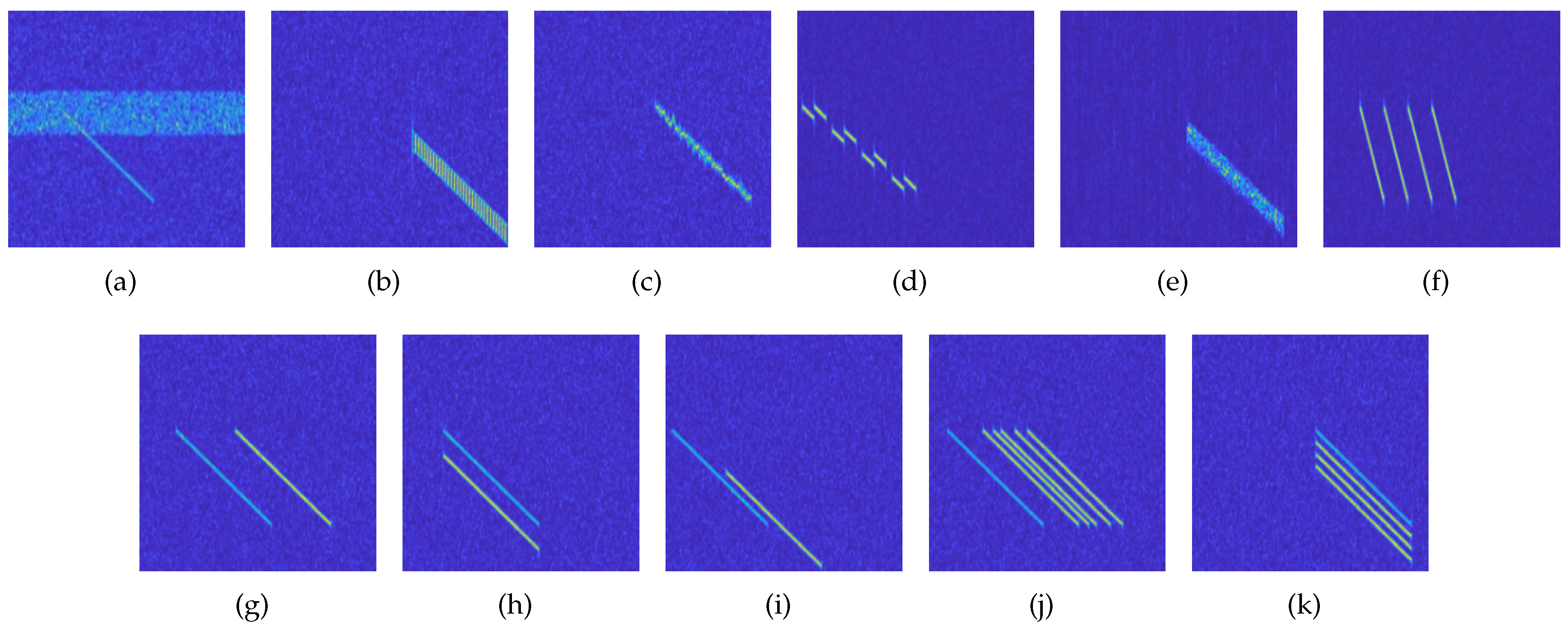
Figure 2.
Schematic diagram of closed-set and open-set tasks.
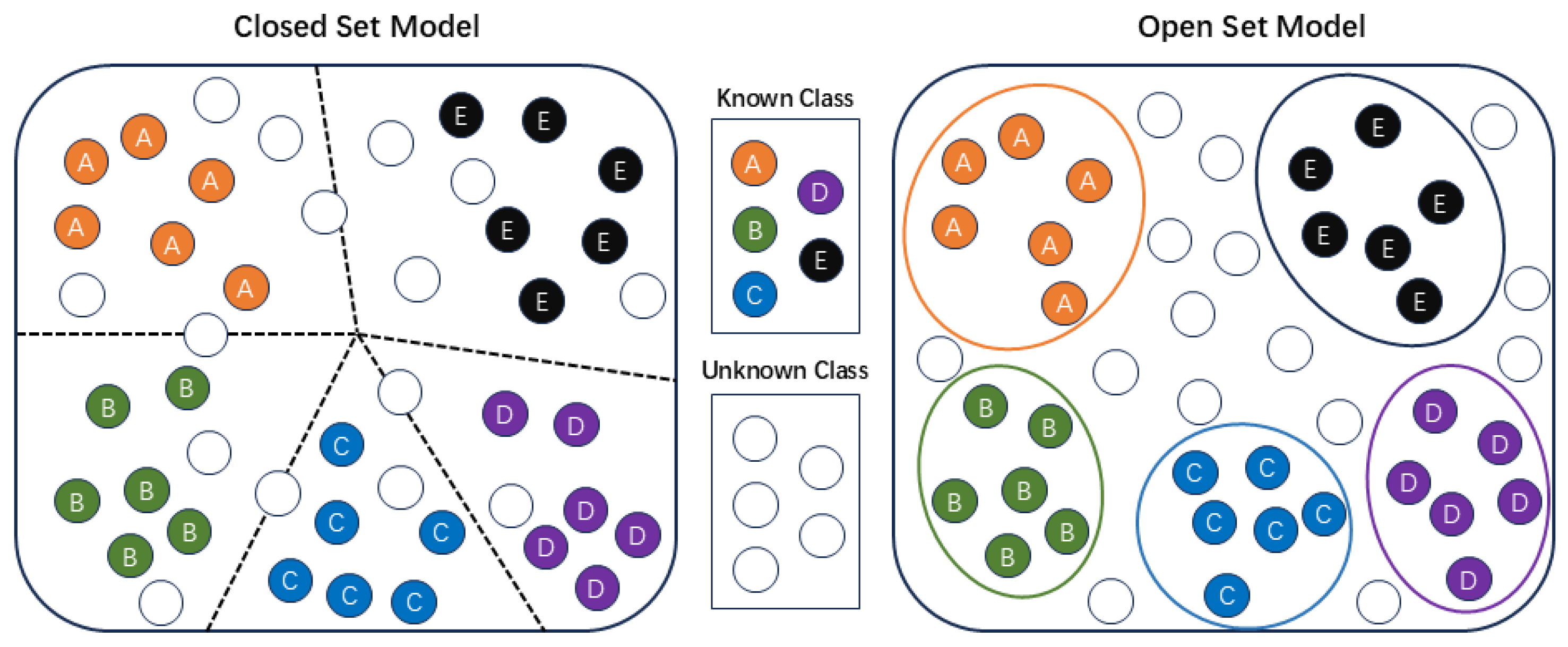
Figure 3.
Framework of the feature extraction network.
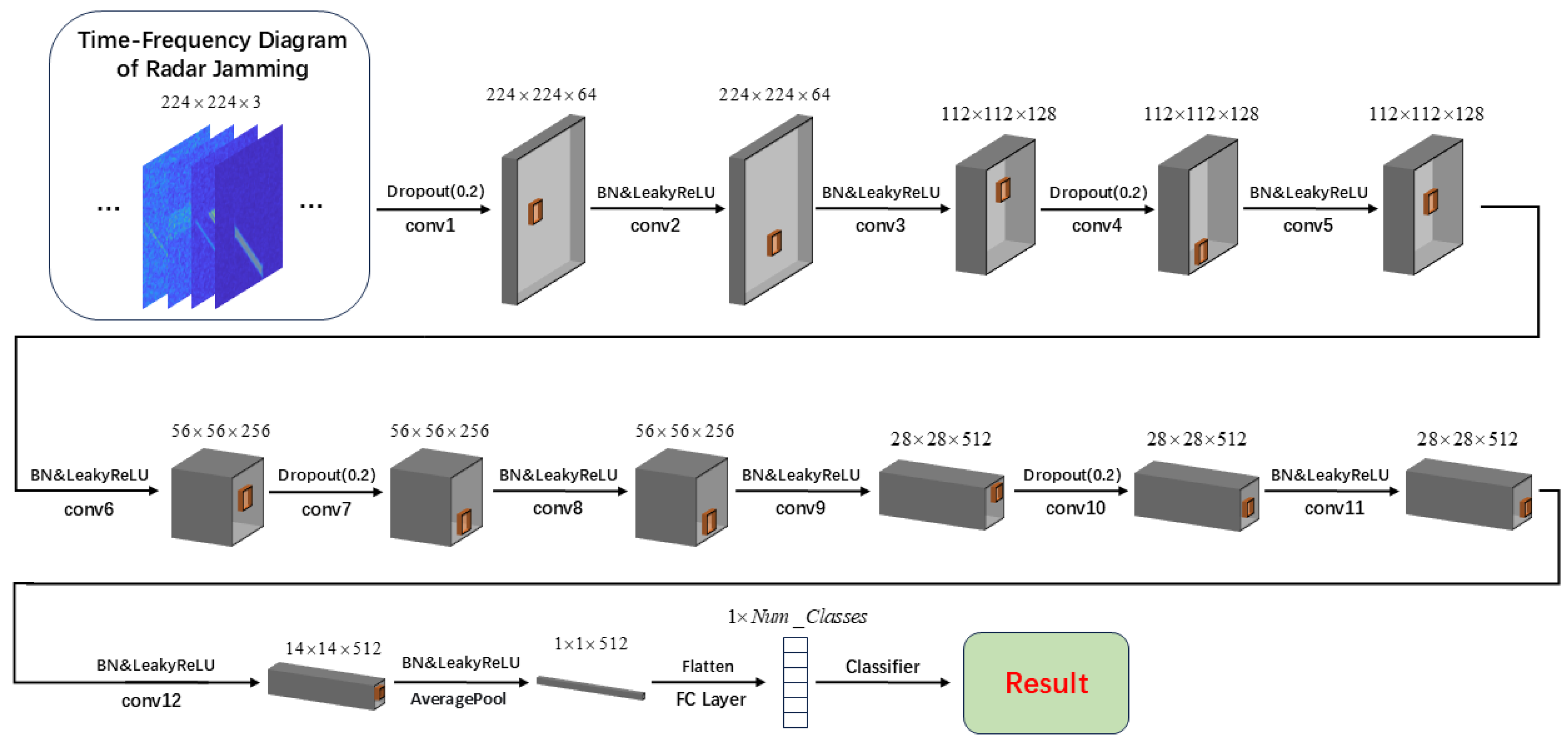
Figure 4.
The feature space of known class distributions optimized by ICL and IBL.
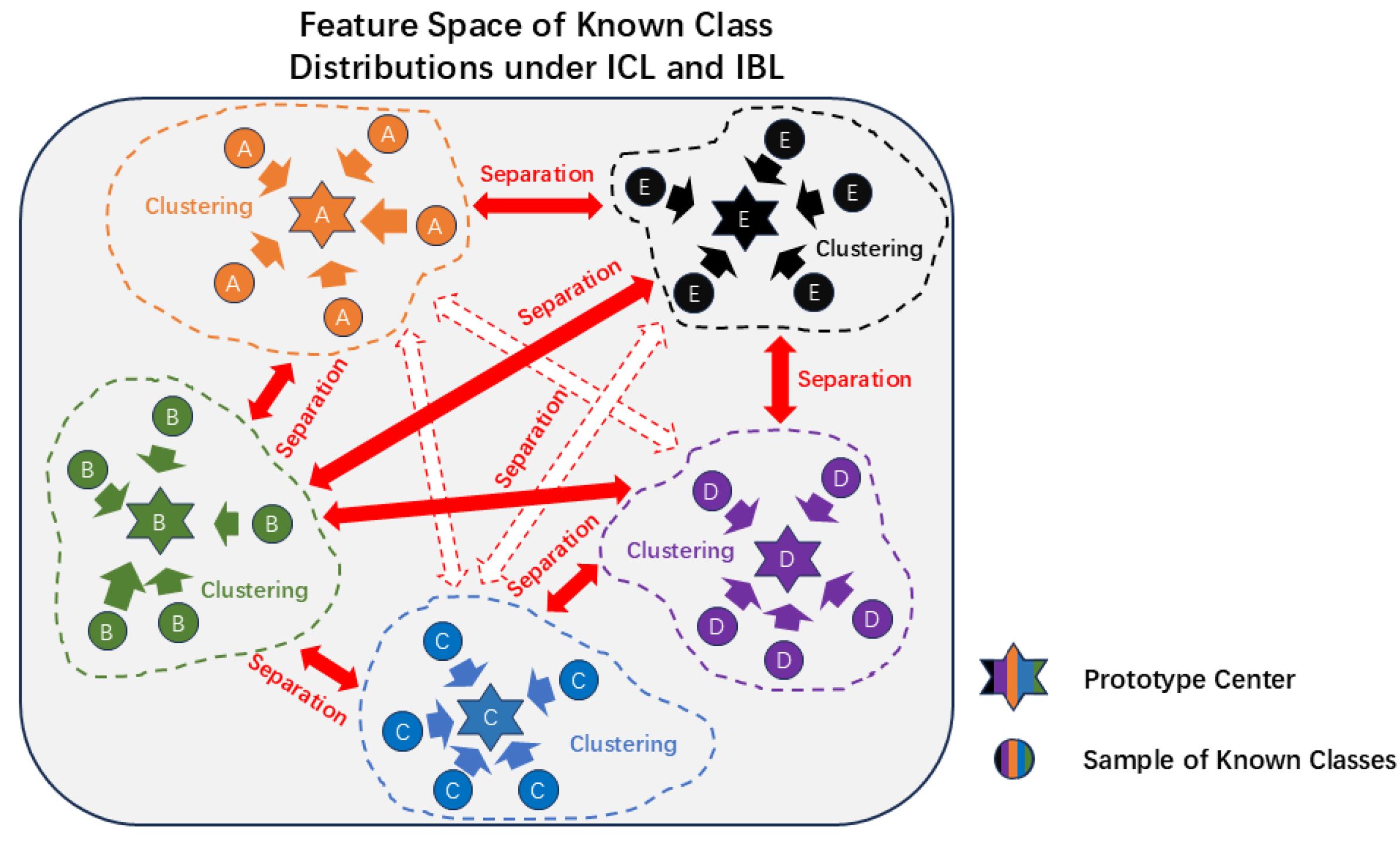
Figure 5.
Schematic diagram of open point learning.
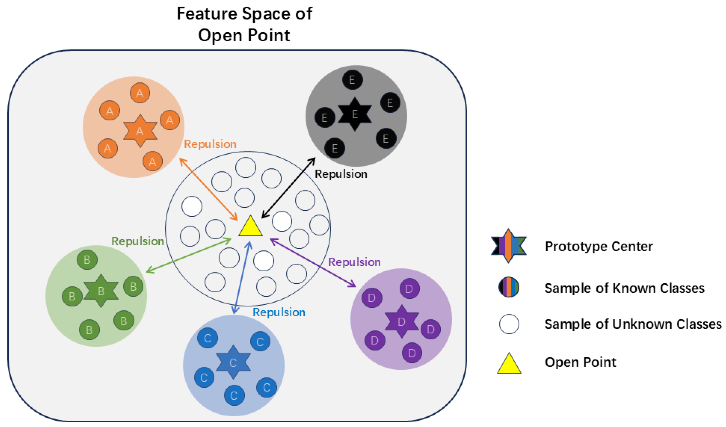
Figure 6.
Comparison diagram of prototype points and reciprocal points.
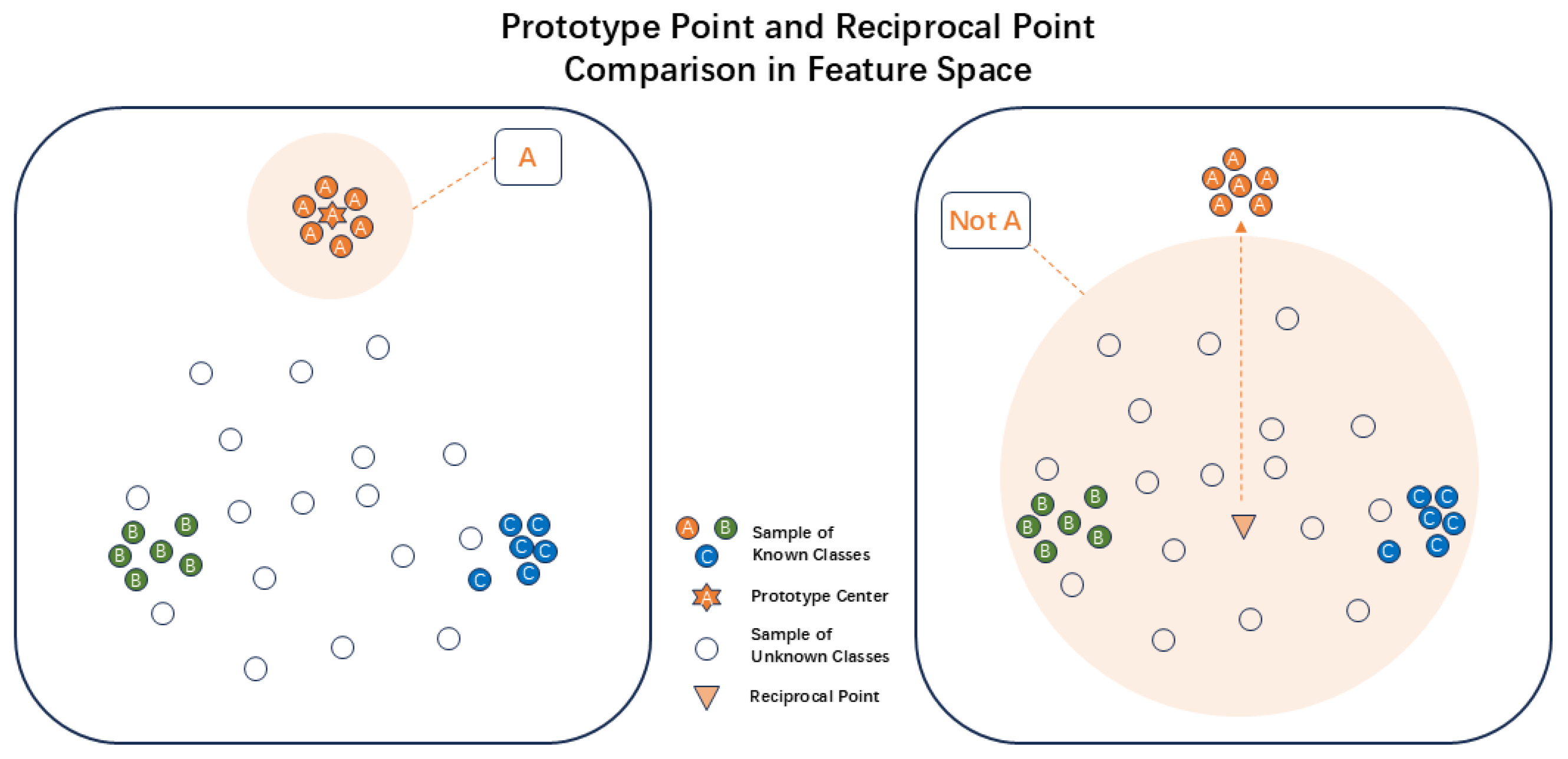
Figure 7.
Feature space mapping before and after ARPL training.
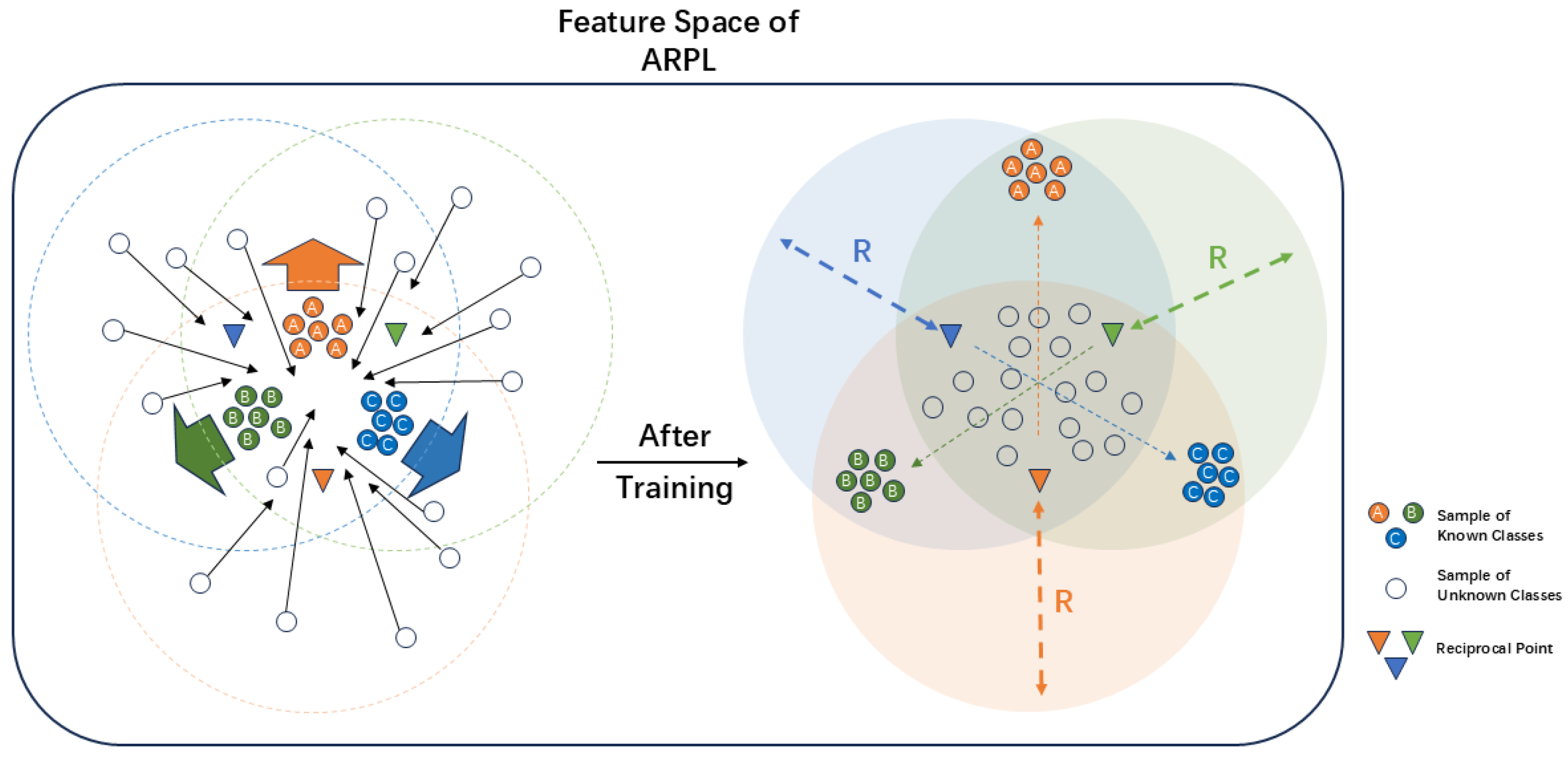
Figure 8.
The principle and feature space learning process of MDPAR.
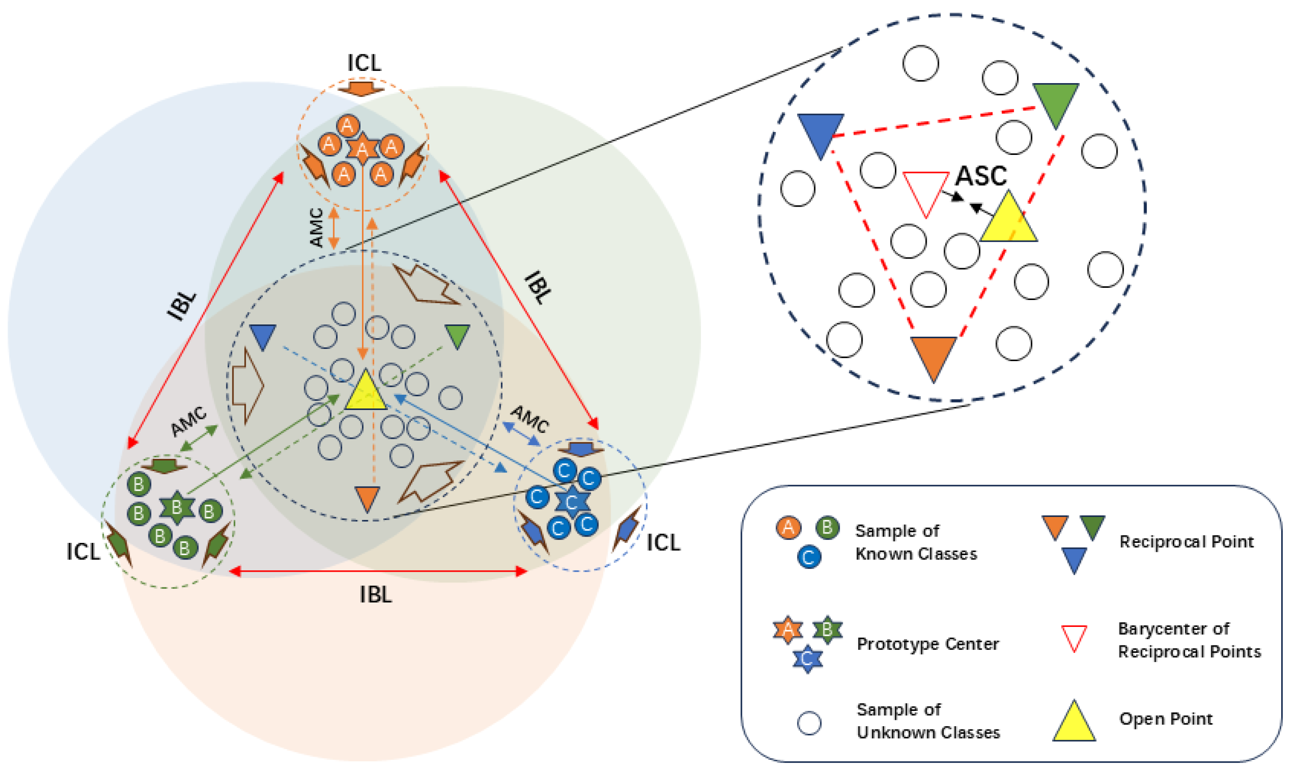
Figure 9.
Overall algorithmic workflow.
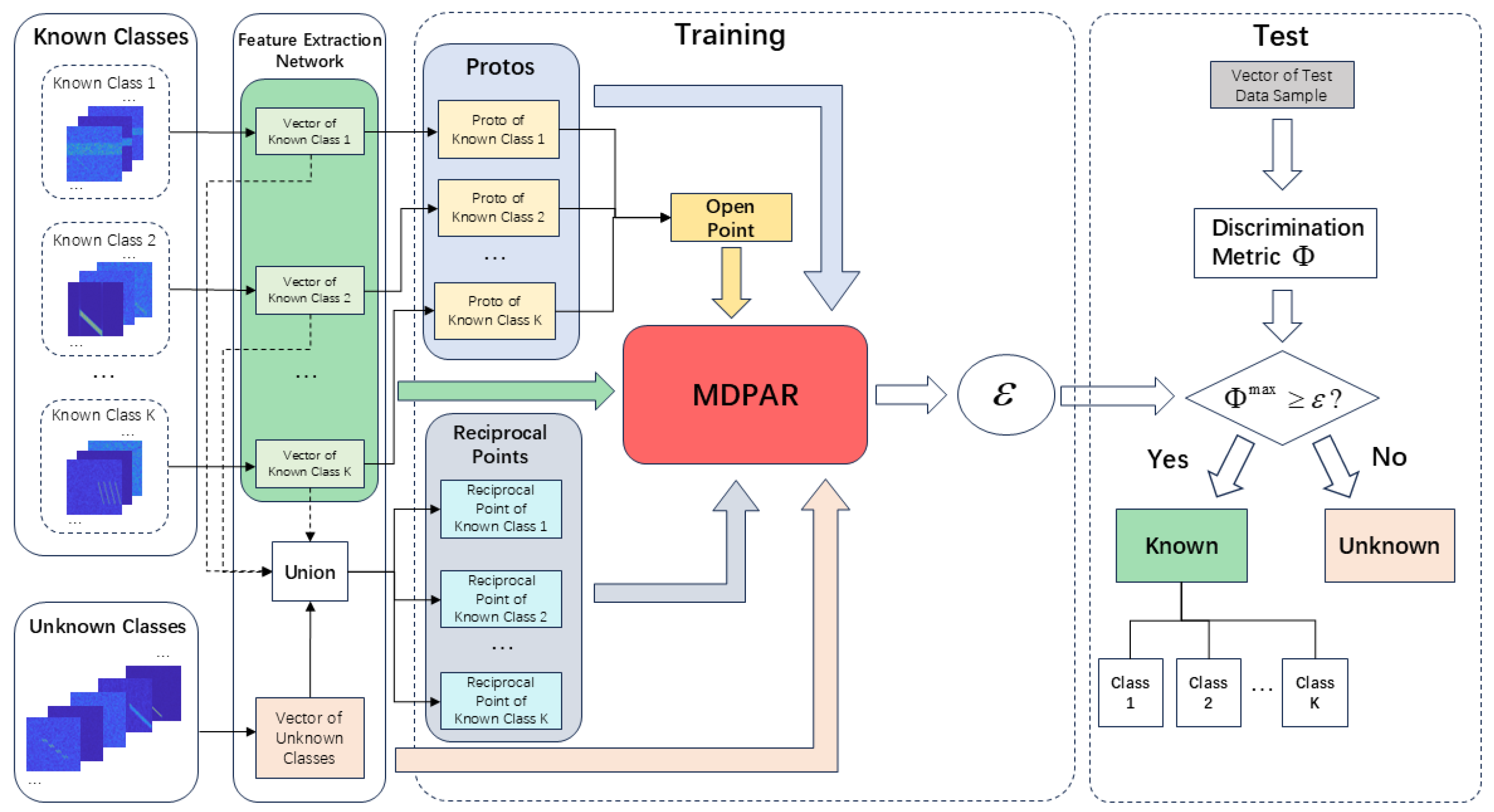
Figure 10.
Changes in open-set metrics of the MDPAR method under different SNRs.
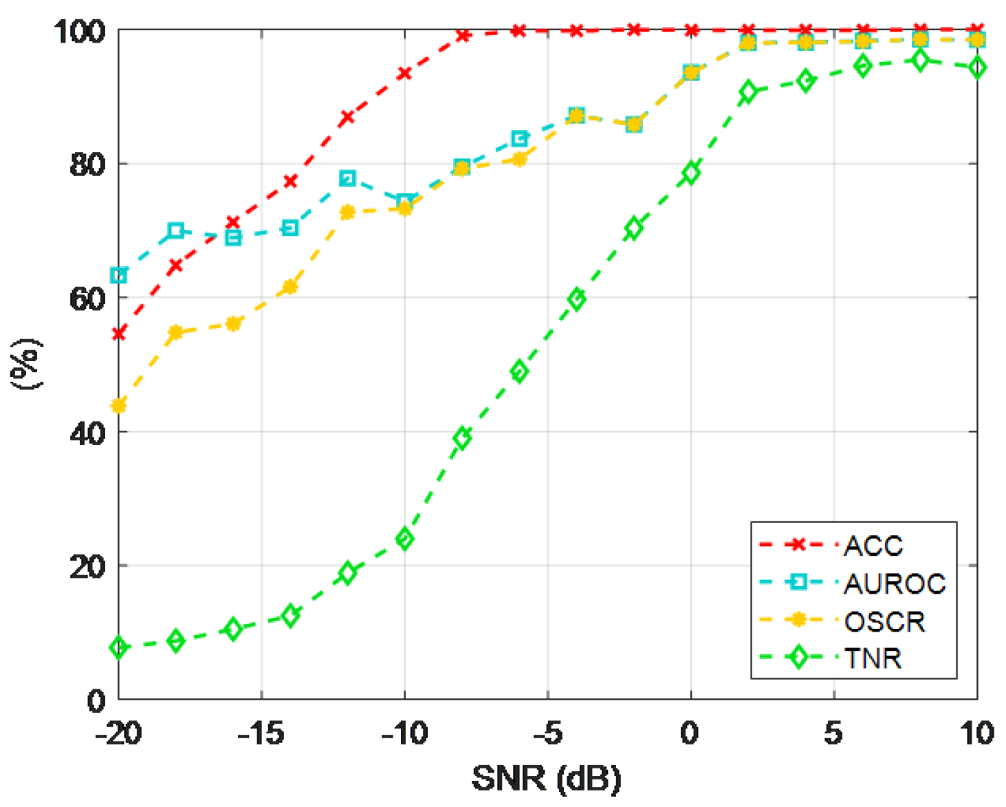
Figure 11.
Histograms of the comprehensive discrimination metric distances for jamming samples using the MDPAR method under different SNRs: (a) -16dB; (b) -8dB; (c) 0dB; (d) 8dB.
Figure 11.
Histograms of the comprehensive discrimination metric distances for jamming samples using the MDPAR method under different SNRs: (a) -16dB; (b) -8dB; (c) 0dB; (d) 8dB.
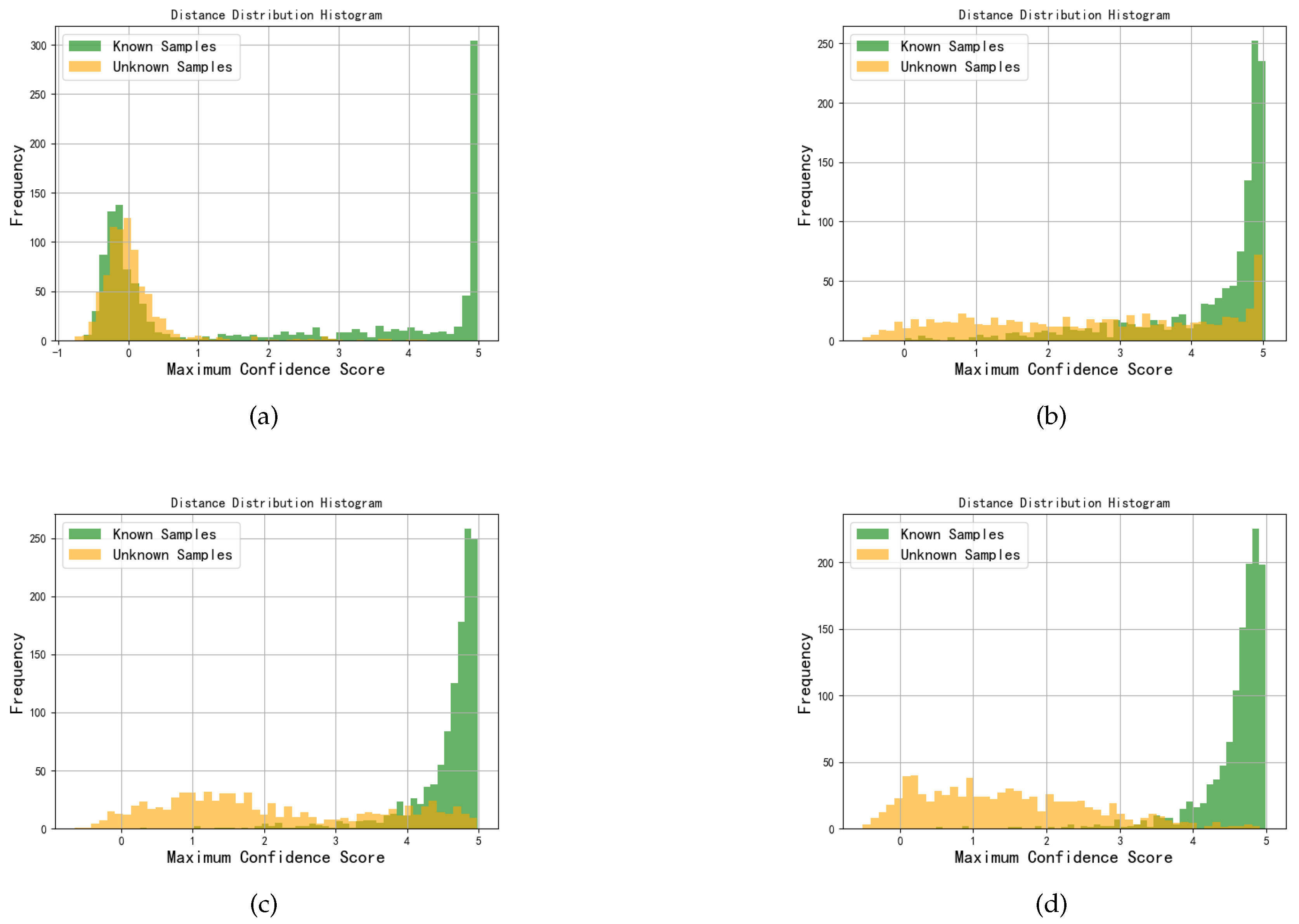
Figure 12.
ROC curves for OSR using the MDPAR method under different SNRs: (a) -16dB; (b) -8dB; (c) 0dB; (d) 8dB.
Figure 12.
ROC curves for OSR using the MDPAR method under different SNRs: (a) -16dB; (b) -8dB; (c) 0dB; (d) 8dB.
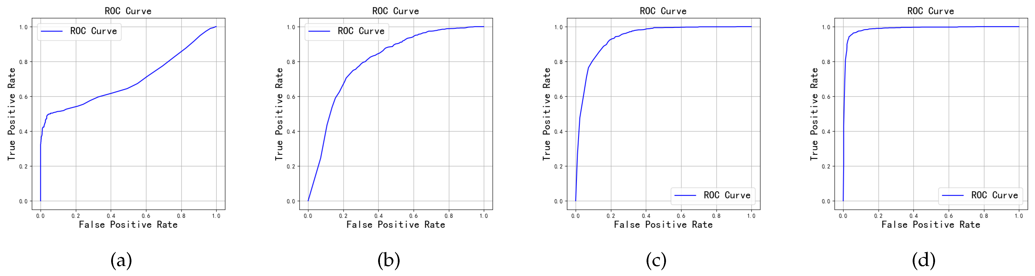
Figure 13.
Visualization of feature vector distributions for OSR using the MDPAR method under different SNRs: (a) -16dB; (b) -8dB; (c) 0dB; (d) 8dB.
Figure 13.
Visualization of feature vector distributions for OSR using the MDPAR method under different SNRs: (a) -16dB; (b) -8dB; (c) 0dB; (d) 8dB.
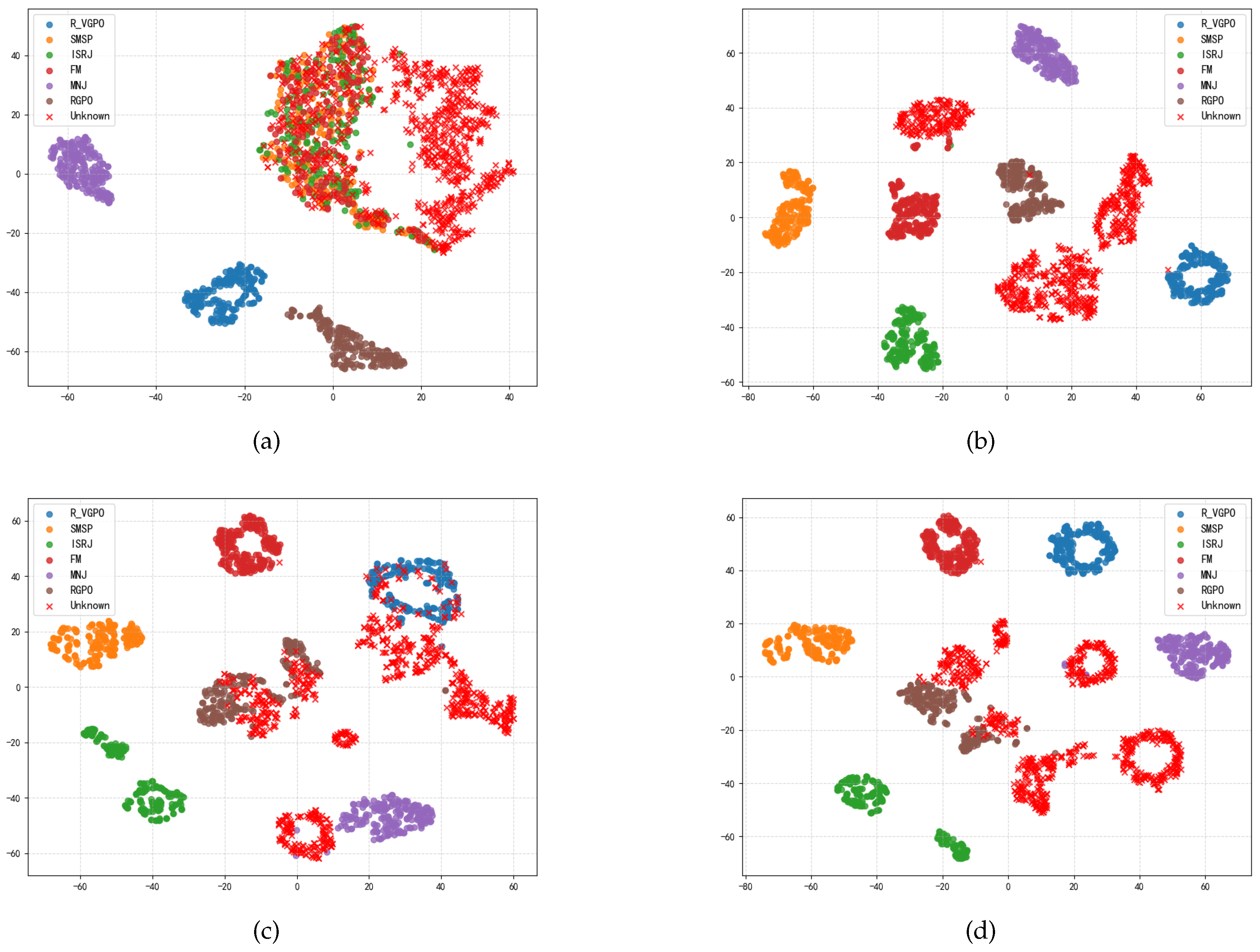
Figure 14.
Confusion matrices for the classification results of known jamming signals using the MDPAR method under different SNRs: (a) -16dB; (b) -8dB; (c) 0dB; (d) 8dB.
Figure 14.
Confusion matrices for the classification results of known jamming signals using the MDPAR method under different SNRs: (a) -16dB; (b) -8dB; (c) 0dB; (d) 8dB.
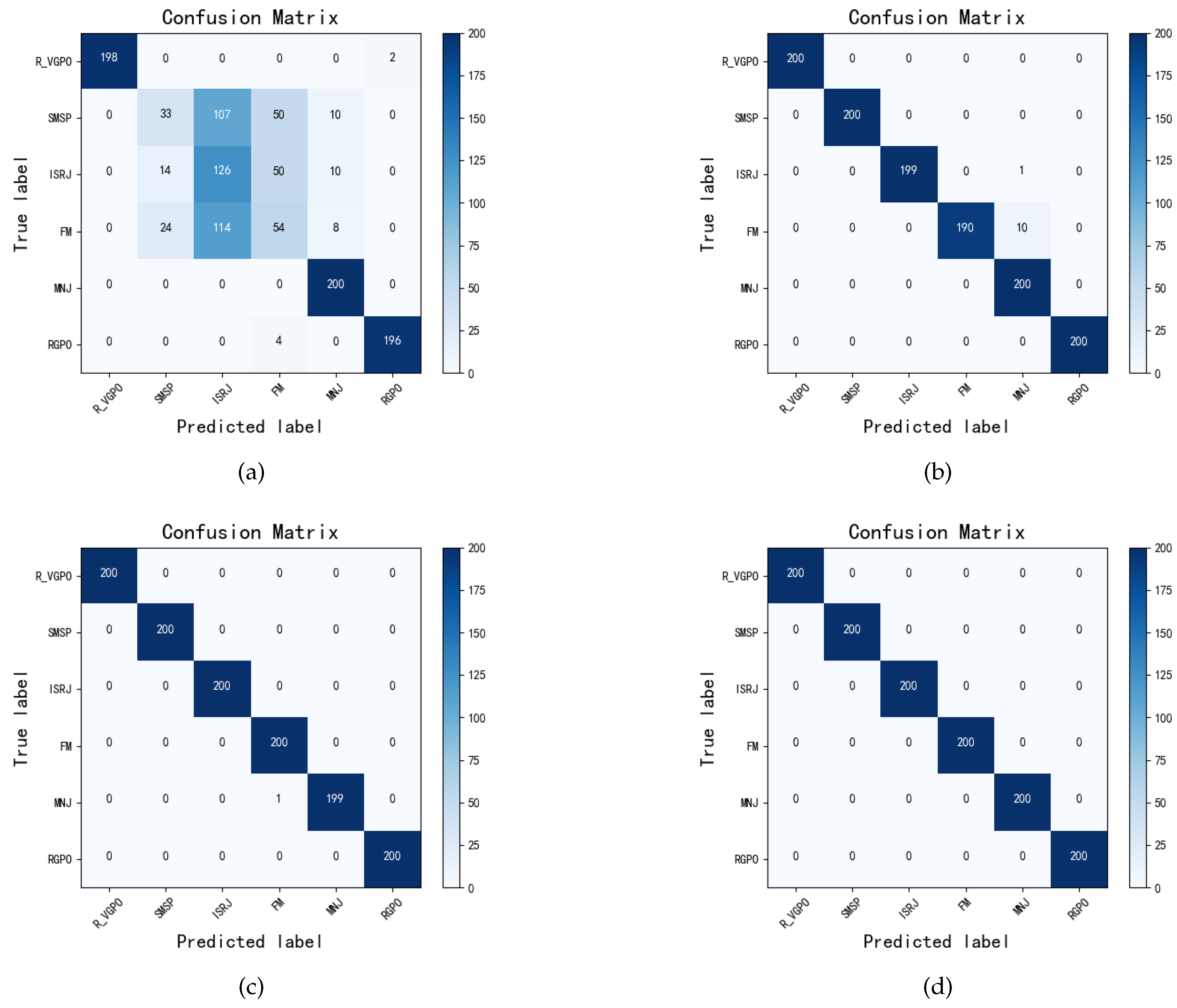
Figure 15.
Changes in MDPAR open-set metrics with openness under different SNR conditions: (a) TNR; (b) AUROC; (c) OSCR.
Figure 15.
Changes in MDPAR open-set metrics with openness under different SNR conditions: (a) TNR; (b) AUROC; (c) OSCR.
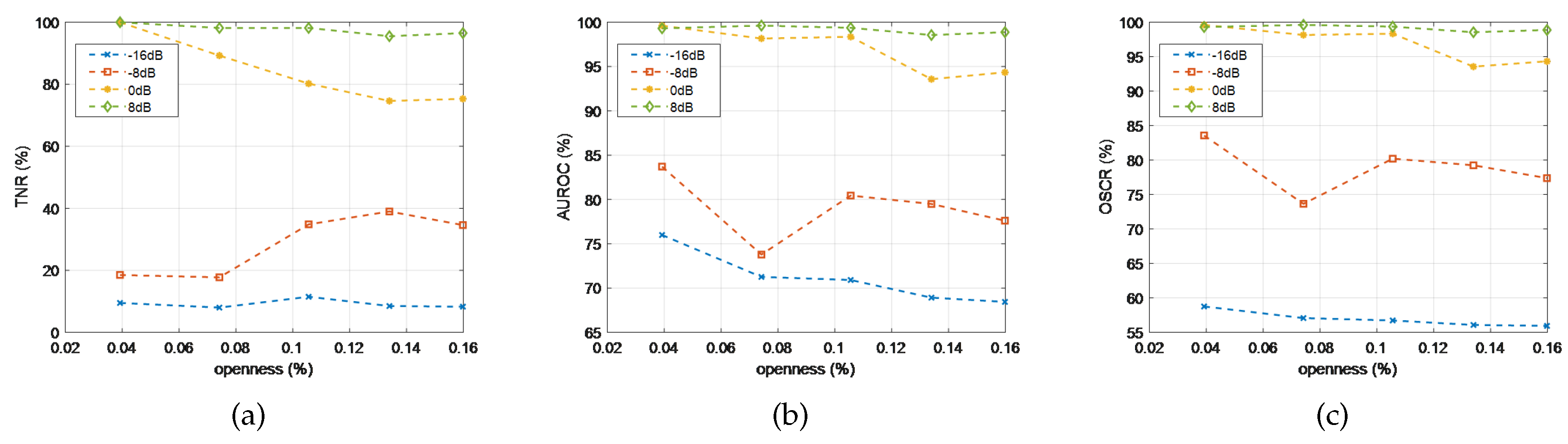
Figure 16.
Histograms of comprehensive discrimination metric distances for samples under different values of : (a) =0.1; (b) =0.3; (c) =0.5; (d) =0.7.
Figure 16.
Histograms of comprehensive discrimination metric distances for samples under different values of : (a) =0.1; (b) =0.3; (c) =0.5; (d) =0.7.
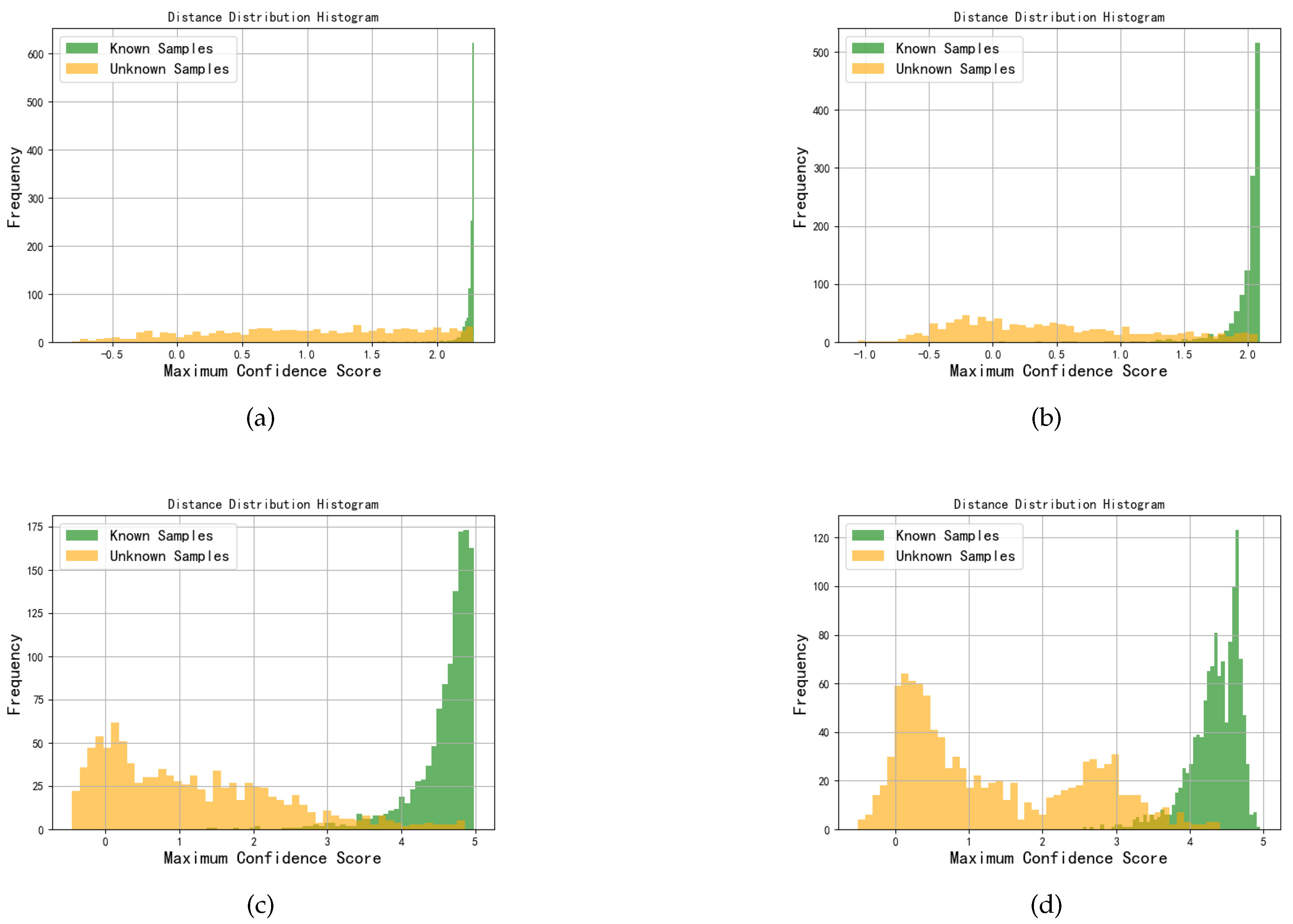
Figure 17.
Differences in feature vector distributions for OSR using the MDPAR method under 0dB with different values of : (a) =0; (b) =0.1; (c) =0.2; (d) =0.4.
Figure 17.
Differences in feature vector distributions for OSR using the MDPAR method under 0dB with different values of : (a) =0; (b) =0.1; (c) =0.2; (d) =0.4.
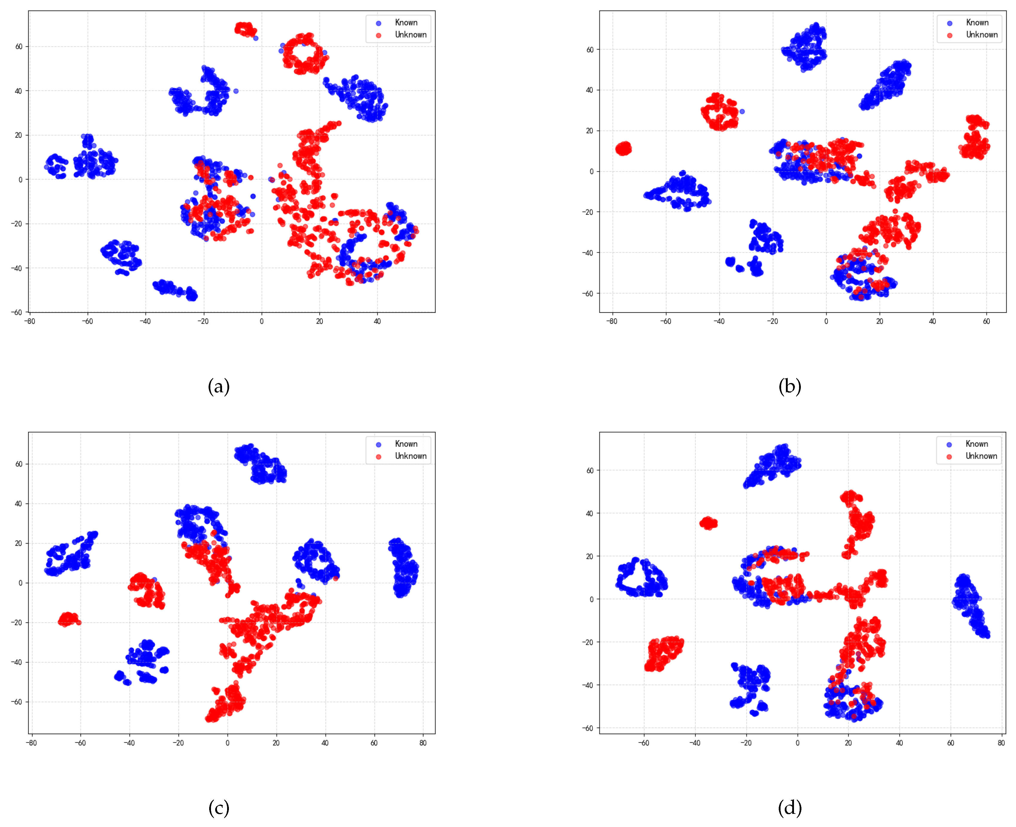

Table 1.
Basic parameter settings for the simulation of transmitted signals and active jamming signals.
Table 1.
Basic parameter settings for the simulation of transmitted signals and active jamming signals.
| Signal Type | Signal Parameter | Parameter Range |
|---|---|---|
| LFM | Sampling Frequency | 100MHz |
| Signal Bandwidth | 40MHz | |
| Center Frequency | 20MHz | |
| Pulse Repetition Interval(PRI) | 100s | |
| Pulse Width | 40s | |
| Signal-to-Noise Ratio(SNR) | -20dB ∼ 10dB | |
| Chirp Rate | MHz/s | |
| Jamming-to-Signal Ratio(JSR) | 5dB | |
| AM | Amplitude Coefficient | [2,3,4] |
| Jamming Bandwidth | 30 ∼ 50MHz | |
| CJ | Number of Comb Subbands | [9,10,11,12] |
| Comb Subbands Amplitude Coefficient | [0.5, 0.6, 0.7] | |
| Comb Subbands Modulation Slope | [0.05, 0.06, 0.08] MHz/s | |
| FM | Noise Bandwidth | [6,8,10] MHz |
| FM Chirp Slope | [1.2,1.4,1.6,1.8] MHz/s | |
| Noise Amplitude | [1,1.4,1.7,2] | |
| Effective Modulation Index | [2,4,6,8] | |
| ISRJ | Sampling Pulse Periods | [4,5,10]s |
| Repetition Times | [4,2,1] | |
| Duty Cycle Values | [20,25,33.33,50]% | |
| Sampling Pulse Width | 1 ∼ 10s | |
| MNJ | Noise Bandwidth | [3,4,6,7] MHz |
| Noise Center Frequency | 20 MHz | |
| SMSP | Sampling Multiples | [3,4,5] |
| RGPOJ,VGPOJ,R-VGPO | RGPO Start Time | 15.5s |
| RGPO Velocity | 100 ∼ 400 m/s | |
| RGPO Duration | 40s | |
| Initial VGPO Velocity | 100 ∼ 300 m/s | |
| VGPO Acceleration | 50 ∼ 500 m/s2 | |
| RMTJ,VMTJ | False Target Delay | 2 ∼ 20s |
| False Target Doppler Shift | 2 ∼ 15 MHz | |
| Number of False Targets | [2,3,4,5] | |
| Inter-False-Target Delay | 1 ∼ 5s | |
| Inter-False-Target Doppler Shift | 1 ∼ 5 MHz |
Table 2.
Experiment setting.
| Params | Value |
|---|---|
| Known Classes | FM,MNJ,ISRJ,SMSP,RPGO,R-VGPO |
| Unknown Classes | AM,CJ,VGPO,RMT,VMT |
| 0.5 | |
| 0.1 | |
| Learning Rate | 0.003 |
| Epoch | 60 |
| Batch Size | 128 |
| Step Size | 30 |
| 0.95 | |
| 0.1 | |
| 0.3 |
Table 3.
Performance comparison of different OSR algorithms.
| Algorithm | SNR(dB) | TNR(%) | ACC(%) | AUROC(%) | OSCR(%) |
|---|---|---|---|---|---|
| OpenMax | -16 | 3.26 | 55.42 | 63.03 | 49.20 |
| -8 | 21.86 | 79.45 | 72.12 | 73.95 | |
| 0 | 63.10 | 92.55 | 88.78 | 81.65 | |
| 8 | 87.33 | 94.45 | 91.24 | 94.12 | |
| RCAE-OWR | -16 | 6.12 | 60.55 | 63.47 | 53.29 |
| -8 | 28.35 | 90.33 | 75.88 | 76.95 | |
| 0 | 72.45 | 96.98 | 90.45 | 89.77 | |
| 8 | 94.12 | 98.67 | 94.56 | 95.89 | |
| MDPAR | -16 | 7.89 | 67.25 | 71.26 | 57.08 |
| -8 | 39.00 | 95.08 | 79.49 | 79.24 | |
| 0 | 75.30 | 99.92 | 94.35 | 94.33 | |
| 8 | 95.50 | 100.00 | 98.56 | 98.55 |
Disclaimer/Publisher’s Note: The statements, opinions and data contained in all publications are solely those of the individual author(s) and contributor(s) and not of MDPI and/or the editor(s). MDPI and/or the editor(s) disclaim responsibility for any injury to people or property resulting from any ideas, methods, instructions or products referred to in the content. |
© 2025 by the authors. Licensee MDPI, Basel, Switzerland. This article is an open access article distributed under the terms and conditions of the Creative Commons Attribution (CC BY) license (http://creativecommons.org/licenses/by/4.0/).
Copyright: This open access article is published under a Creative Commons CC BY 4.0 license, which permit the free download, distribution, and reuse, provided that the author and preprint are cited in any reuse.


