Submitted:
20 March 2025
Posted:
20 March 2025
You are already at the latest version
Abstract
Artificial ocean alkalinization (AOA) is one of the most promising marine carbon dioxide removal technologies. We applied the results from the 6th Coupled Model Intercomparison Project (CMIP6) to characterize the temporal and spatial variabilities of future marine carbon chemistry under the implementation of AOA. Our study shown the carbon system varied widely under the implement of AOA, but some efficiencies may be covered up by the forcing of high carbon emission scenario. Basing on the CMIP6 protocol, which added 0.14 Pmol alkalinity into the ocean ever year, AOA promoted the increase of DIC, delayed the rise of pCO2, and restrained the aggravation of pH and Ω, actually. The temperate oceans in both hemispheres were the most significant impacted basins, whereas the Southern Ocean were the less affected region. In the present century, the oceanic carbon sink would intensify rapidly until the year around 2080, and then weaken slowly. Implementation of AOA merely changed the relative strength of oceanic sink rather than its variation pattern. In deep ocean, what’ more, the effectiveness of AOA did exist, but was quite little for the mitigation of ocean acidification.
Keywords:
carbon chemistry
; artificial ocean alkalinization
; earth system model
1. Introduction
Announced by the Sixth Assessment Report of the Intergovernmental Panel on Climate Change (IPCC), the global surface temperature has increased by 1.1°C by 2011-2020 compared to 1850-1900, which is unequivocally caused by human activities through emission of greenhouse gases (GHG) [1]. Climate researches conducted in recent decades find that carbon dioxide (CO2), the uppermost contributors for GHS, is higher than at any time in the past 200,000 years of human history, which has already break through the concentration of 420 μatm in the end of 2024. And the historical cumulative net emission of CO2 from 1850 to 2019 is estimated to be as much as 2400 ±240 Gt [1] (1Gt =109 t). Consequently, holding temperatures to well below 2 °C, and ideally 1.5 °C above the pre-industrial levels by the end of the century, exactly as the Paris Agreement’s objectives, requires not only rapid reductions of greenhouse gas emissions but removing billions of tons of CO2 from the atmosphere [2].
Marine carbon dioxide removal (mCDR) technologies have recently gained extensive attention because about a quarter of the CO2 emission have been taken up by the ocean sinks since the Industrial Revolution [3,4], and thus the ocean has great influence on the mitigation of climate changes. As a whole, the ocean, serving as the largest pool of reactive carbon, contains about 3800 Gt of dissolved inorganic carbon (DIC), which is imported as a result of the dissolution of atmospheric CO2 into the seawater. Exchange of CO2 between the atmosphere and the ocean mixed layer (roughly the top 100 m of the ocean), regulated basically by the concentration gradient, temperature, and wind speed, is pretty rapid. The characteristic time scale for this air-sea exchange process is on the order of one year. Equation 1 describes what CO2 undergoes after it enters the ocean [5]. The gaseous CO2 firstly transforms into its aqueous form and then forms carbonic acid (H2CO3) (Actually, the aqueous form of CO2 and H2CO3 are hard to distinguish technically). Carbonic acid rapidly dissociates into free hydrogen ion (H+) and bicarbonate (HCO3-). And then, the bicarbonate further dissociates into H+ and carbonate (CO32-) with quite a slow rate. The dissolved species in Equation 1, predominantly in the form of HCO3-, make up the carbonate alkalinity system, the dominant contributor to seawater alkalinity. Alkalinity, roughly refers to the excess of proton acceptors over donors, is a marine chemical parameter that largely determines the buffer capacity for CO2 in seawater (Equation 2) [6]. Basing on the above-mentioned ocean carbon chemistry, the concept of artificial ocean alkalinization (AOA) is put forward. AOA is considered as one of the most promising mCDR methods that has a theoretical sequestration potential in the range of 3 to 30 Gt CO2 yr−1 ([7,8,9]). Increasing alkalinity drives consumption of protons and production of bicarbonate (HCO3−) and carbonate (CO32−), which leads to a corresponding increase of pH and a following decrease of partial pressure of CO2 (pCO2) in seawater. These above changes would finally promote CO2 uptake from the atmosphere via air–sea gas exchange process.
TA = [HCO3-] + 2[CO32-] + [B(OH)4-] + [OH-] + [HPO42-] + 2[PO43-] + [H3SiO4-] + [NH3] + [HS-] – [H+]F – [HSO4-] -[HF] – [H3PO4] + ... - ...
Previous studies have explored some aspects of AOA. For example, basing on an ocean carbon cycle model, Ilyina et al. [10] confirmed that intensive enhancement of ocean alkalinity had the potential to promote oceanic uptake of fossil fuel CO2 from the atmosphere and could avoid further ocean acidification indeed. Feng et al. [11] run AOA simulations in the Great Barrier Reef, Caribbean Sea and South China Sea by an Earth system model of intermediate complexity, and founded alkalinization could counteract the local acidification changes expected in 21st century, in aspects of both oceanic surface pCO2 and surface aragonite saturation (Ω). However, Keller at al. [12] found the effectiveness of AOA was actually limited by the production ability and the transport capacity of alkalinity material. So, the practical AOA induced atmospheric CO2 reduction under current conditions was relatively small compared with the expected business-as-usual CO2 emissions, and as a result, the atmospheric CO2 would continue to increase gradually. Zhou et al. [13] presented the global maps of AOA efficiency, and found that the equilibration kinetics had two characteristic timescales: rapid surface equilibration followed by a slower second phase. These kinetics vary considerably with latitude and the season of alkalinity release.
At present, there seems to be little consensus about the climate impacts and marine response of AOA, especially under the background of continuous rising carbon emission. Methodologically, the AOA implementation could be obtained by both observation-based estimations [e.g. 14,15,16] and model simulation outputs [e.g. 17,18,19]. But in a way, model simulation can compensate for the inevitable temporal-spatial limitation of observation-based methods. The Earth System Models (ESMs) are the latest generation of the state-of-the-art climate models, which couple the carbon cycle processes among the atmosphere, land, and ocean, and simulate the real earth systems to the maximum extent. Therefore, the ESMs could serve as a helpful and powerful tool to analyze and diagnose the AOA.
To address this, we apply the up-to-date datasets produced by the new versions of ESM from the 6th Coupled Model Intercomparison Project (CMIP6) to characterize the temporal and spatial variabilities of marine carbon chemistry under the implementation of AOA. This paper will provide the comprehensive fundamental information of the CMIP6 AOA experiment, present the variabilities of the four most important carbonate chemistry parameters (DIC, pH, pCO2 and Ω), and estimates the long-term average and future tendency of air-sea CO2 exchange flux (FCO2). The remainder of this paper is organized as following. Section 2 introduces the model, datasets, and analytical materials. The results and discussions are presented in Section 3. Section 4 makes the conclusion.
2. Materials and Methods
We use the NorESM2-LM model in this study, which is the second generation of the fully coupled Earth system model developed by the Norwegian Climate Center [20]. For details, the atmosphere component of NorESM2-LM is built on the Community Atmosphere Model version 6 (CAM6) but with particulate aerosols and the aerosol-radiation-cloud interaction parameterization, which is referred to as the CAM6-Nor. The ocean component is the Bergen Layered Ocean Model (BLOM), which employs an isopycnic vertical coordinate, with near-isopycnic interior layers and variable density layers in the surface mixed boundary layer [20]. The ocean biogeochemistry component of NorESM2-LM is adapted from the HAMburg Ocean Carbon Cycle model and was converted to isopycnic coordinate (iHAMOCC) [21]. The sea ice model component is based upon the Community Ice CodE (CICE) sea ice model [22]. What’s more, the NorESM2-LM employs the latest version of Community Land Model (CLM5) as the land component [23].
Data analyzed in this study are derived from the monthly outputs of three CMIP6 experiments: the esm-hist, the esm-ssp585, and the esm-ssp585-ocn-alk [24,25]. Briefly, The CMIP6 esm-hist simulation, in which the atmospheric CO2 concentration is calculated according to the historical anthropogenic CO2 emissions forcing, is essential for the reliability testing before the ocean alkalinization experiment. This experiment is run from the year of 1850 to 2014. The esm-ssp585, then, is driven by the SSP5-8.5 high CO2 emission scenario and run from the end year of esm-hist simulation until the end of this century (2015 to 2100), and serves as the control run and branching point for the subsequent ocean alkalinization experiment. The esm-ssp585-ocn-alk simulation, forcing by the SSP5-8.5 high CO2 emission scenario as well, adds 0.14 Pmol TA (1 Pmol=1015 mol) to the upper ice-free ocean surface waters between 70°N and 60°S every year during from 2015 to 2100. In general, the average differences between the AOA esm-ssp585-ocn-alk and the no-AOA esm-ssp585 of specific parameters are obtained as the net effectiveness of AOA implement. What’s more, the key information about the CMIP6 experiments conducted by the NorESM2-LM is summarized in Table 1 as below.
Observational dataset employed in this paper is the classic climatological air-sea CO2 flux from Lamont-Doherty Earth Observatory of Columbia University with the original resolution of 4°×5° [26], which was widely used in the study of global carbon cycle. We re-gridded it into 1°×1° grid and referred to it as “Takahashi2009” for the comparison of long-term average air-sea CO2 flux and spatial distributions of model bias.
3. Results and Discussion
3.1. Performance of the model simulation
The simulated global air-sea CO2 flux in the NorESM2-LM esm-his experiment is compared with the observational result of Takahashi2009 to assess the general performance of the model (Figure 1). The result indicates the model could generally reproduce the dominant patterns of Takahashi2009: the equatorial Pacific is the major oceanic CO2 source for atmosphere, and the temperate oceans in both hemispheres are the major oceanic sinks for atmospheric CO2 with the North Atlantic is the most intensive CO2 sink. What’s more, the long-term average annual net uptake flux of CO2 by the global oceans has been estimated to be 2.05 PgC yr-1 for the NorESM2-LM model, which is exactly in accordance with the climatological results of Takahashi et al. [26,27] (1.6 to 2.2 PgC yr-1). What’s more, Qu et al. [28] had assessed the long-term average and spatial-temporal variability of global air-sea CO2 exchange flux (FCO2) since 1980s basing on the results of 18 CMIP6 ESMs. They found the NorESM2-LM performed particularly well comparing with the other CMIP6 ESMs because its root-mean-square error (RMSE) with respect to the observation result was quite low among the 18 CMIP6 ESMs. These consistencies arguably indicate that the NorESM2-LM performs fairly well in simulating the mean state of global air-sea CO2 exchange process. As a result, we could apply its following result of esm-ssp585 and esm-ssp585-ocn-alk for further investigate reasonably.
3.2. Variations of the marine carbon system during AOA
Generally, the carbonate system can be described by six fundamental parameters in thermodynamic equilibrium: DIC, TA, [CO2], [HCO3-], [CO32−], and pH. The concentrations of OH− and pCO2 can be readily calculated using the dissociation constant of water and Henry’s law [5]. Given the first and second dissociation constants of carbonic acid and the definitions of DIC and TA, the marine carbon system can be constrained by knowing simply two carbonate chemistry parameters, except temperature, salinity, and pressure. In order to depict the variations of marine carbon system under the implementation of AOA more comprehensively, we investigate four important marine carbon parameters, except TA, simulated by the esm-ssp585-ocn-alk experiment, and compared them with those from the esm-ssp585 experiment. They are DIC, pCO2, pH, and Ω. It is worth pointing out that, DIC and pCO2 are usually adopted to characterize the budgets of oceanic carbon source/sink and Ω and pH are used to reveal the feature of ocean acidification. In our article, the trend of a specific carbon chemistry parameter is calculated on gridded monthly data using ordinary least squares (OLS) regression. And the time series of a parameter is calculated by the area weight mean value of global gridded data.
Overall, the implementation of AOA indeed changed the response of marine carbon sysem on the ever growing carbon emission significantly. Simultated by the esm-ssp585-ocn-alk experiment conducted by the NorESM2-LM, the global-averaged concentrations of DIC and pCO2 increased obviously in the rates of 2.54 μmol·kg-1·yr-1 and 6.80 μatm·yr-1 during the period of 2015 to 2100 (Figure 2a and 2b), respectively, while the pH and Ω decreased clearly in the rates of -0.041 yr-1 and -0.0156 yr-1, respectively (Figure 2c and 2d). The raised concentrations of DIC and pCO2 were easy to explain, because the addion of alkalinity contains abundant carbon in the form of [HCO3-] or [CO32-].
However, the paradoxical results of pH and Ω after AOA seemd perverse (enhanced TA but aggravated acidifation). We attributed this results to the inadequacy of alkalinization with respect to the carbon emission budget. In the CMIP6 project, the esm-ssp585-ocn-alk experiment was also driven by the SSP5-8.5 high CO2 emission scenario. Shared Socioeconomic Pathways (SSPs) are climate change scenarios of projected socioeconomic global changes up to 2100 as defined in the IPCC Sixth Assessment Report on climate change in 2021. SSP5-8.5 is a very high greenhouse gas emissions scenario where CO2 emissions triple by 2075 and the concentration of atmospheric CO2 is estimated to be as high as more than 1100 μatm in 2100 [29]. The CMIP6 esm-ssp585-ocn-alk experiment adds 0.14 Pmol TA to the upper ice-free ocean surface waters between 70°N and 60°S every year during from 2015 to 2100. The aforementioned results of pH and Ω just implied that the AOA with the intensity of esm-ssp585-ocn-alk experiment in CMIP6 could not counteract the effects of the SSP5-8.5 high CO2 emission. As a matter of fact, the original intention of esm-ssp585-ocn-alk experiment was not to test the maximum potential of AOA, which would be difficult given the the way in which ocean carbonate chemistry is simulated, but rather to compared the response of models to a significant alkalinity perturbation [12]. Nevertheless, if we compared the esm-ssp585-ocn-alk experiment with the esm-ssp585 experiment without AOA measurements (blue dash line in Figure 2), it could be detected explicitly that the AOA promoted the increase of DIC, delayed the rise of pCO2, and restrained the aggravation of pH and Ω, actually (Figure 2).
As for the spatial features of changes in surface distributions of marine carbon system, we calculated the differences between the AOA esm-ssp585-ocn-alk experiment and the no-AOA esm-ssp585 experiment, and present its long-term average results in a global perspective in Figure 3. It was conspicuously that, under the background of high CO2 emission scenario, the implementation of AOA was able to induce increases of DIC, pH, and Ω, and reduction of pCO2, globally (Figure 3a-d). It needs to be specifically pointed out that these above mentioned “increase” and “decrease” were relative to the no-AOA esm-ssp585 of course. In terms of spatial distribution, the temperate oceans in both hemispheres were the most significant impacted basins, whereas the Southern Ocean were the less affected region. This spatial distribution patter had also been confirmed by previous studies [e.g. 10]. To a great extent, this was because the alkalinity was only added into the ice-free ocean surface waters between 70°N and 60°S basing on the CMIP6 protocols. So, the Southern Ocean, which generally located at south of 60° S latitude, should be the least disturbed ocean for AOA before waters affected by alkalinization were transported there by ocean flow and mixing. Nevertheless, some study argued that adding alkalinity to surface waters which would be longer in contact with the atmosphere were more effective in lowering of atmospheric CO2 [10]. So, in view of the circulation pattern and the prevailing Antarctic Circumpolar Current, alkalinization at the Southern Ocean site had the fastest and largest effect on the regional surface carbon system chemistry, whereas alkalinity added in the surface waters in the North Atlantic had only a small effect on the surface carbon system chemistry because the North Atlantic was the area of deep water formation. Furthermore, the spatial patterns in AOA efficiency and its seasonal variation were estimated to be most pronounced at subpolar latitudes in a short time scale (less than 15 years) [2]. By reason of the foregoing, the esm-ssp585-ocn-alk experiment of CMIP6 was able to simulate the overall variation pattern of the marine carbon system during AOA, but the detailed spatial and seasonal variations need further specific modeling.
3.3. Effect of AOA on air-sea CO2 exchange flux
Artificial ocean alkalinization is considered as one of the most promising ocean-based carbon dioxide removal methods. By increasing surface TA, the seawater carbon system equilibrium chemistry moves towards bicarbonate (HCO3-) and carbonate (CO32-), and then the surface pCO2 decreases subsequently, simulating the net transfer of CO2 from the atmosphere to the ocean. This is the marine chemistry fundamental for AOA. In this section, we would present the fffect of AOA on air-sea CO2 exchange flux.
The annual net global air-sea CO2 exchange flux was adopted from the variable of “fgco2” in the no-AOA esm-ssp585 experiment and the AOA esm-ssp585-ocn-alk experiment every CMIP6 model, which means “surface downward mass flux of carbon dioxide expressed as carbon”. We obtained two instructive findings (Figure 4): in the present century, the oceanic carbon sink would intensify observably until the year around 2080, and then slow down gradually. And the implementation of AOA merely changed the relative strength of oceanic sink rather than the above variation pattern. To be specific, the annual air-sea CO2 exchange flux enhanced more rapidly with a rate of (0.061 PgC·yr-2) under the AOA measurement than those without AOA measurement (0.048 PgC·yr-2). After 2080, however, the net sink of the ocean reduced in nearly equal rates of 0.012 to 0.014 PgC·yr-2. We speculated the switch of the ocean CO2 sink occurred around 2080 under the high SSP5-8.5 scenario was probably caused by the variation of ocean-atmosphere dynamics conditions, which was beyond the scope of this article and need further investigation.
Did the addition of 0.14 Pmol TA every year of CMIP6 protocols could lower the atmospheric CO2 concentration under the high SSP5-8.5 scenario? Our results suggested that the effectiveness of AOA did exist, but was quite little (Figure 5). Figure 5 illustrated that the concentrations of atmospheric CO2 increased continuously both for the no-AOA esm-ssp585 (bule), and the AOA esm-ssp585-ocn-alk (orange) during from 2015 to the end of this century. It has been mentioned above that the SSP5-8.5 is a very high greenhouse gas emissions scenario where the concentration of atmospheric CO2 is estimated to be as high as more than 1100 μatm in 2100. Hence, mainly controlled by the ever-increasing carbon emission, the globally averaged atmospheric CO2 concentration rose rapidly, and exceed 1000 μatm around the year of 2100. The AOA project just lower the increase rate for about 0.5 μatm·yr-1 (7.28 minus 7.78). Hence, in simple terms, the supplement of alkalinity material should be increased substantially just for the sake of lowering the atmospheric CO2 concentration under the high SSP5-8.5 scenario.
3.4. Effects of AOA into the ocean interior, take Ω for an example
By increasing TA, the buffering capacity of seawater is enhanced so that seawater pH and CaCO3 saturation degree should increase. However, the relevant results in Section 3.2 indicated that controlled by the ever-increasing carbon emission, the surface pH and Ω actually decreased (e.g. Figure 2c and 2d). Due to the pressure effect, the saturation degree of CaCO3 usually decreases along with the depth of seawater. When Ω is above 1, CaCO3 tends to precipitate, and while below 1, CaCO3 tends to dissolve. So, the concentration of Ω was basically >1 in the surface ocean, but it could be <1 in the deep layer. In this section, we applied the “minimum depth of aragonite undersaturation in seawater”, a parameter simulated by the NorESM2-LM, as an appropriate index to evaluate the effect of AOA into the ocean interior.
Firstly, we calculated the globally mean values of minimum depth of aragonite undersaturation, and presented them in Figure 6. The result shown that the minimum depth of aragonite undersaturation would decrease rapidly under the high SSP5-8.5 scenario, no matter the implement of AOA or not. The implement of AOA merely lowers the decreasing rate for about 0.26 m·yr-1 (-5.04 minus -5.30, in Figure 6). In the year of 2100, the global ocean deeper than about 3900 m would be undersaturated to aragonite, implying the growing problem of ocean acidification under the high SSP5-8.5 scenario. As a result, the Figure 6 suggested that the effectiveness of AOA did exist in deep ocean, but was quite little for the mitigation of ocean acidification.
4. Conclusions
Artificial ocean alkalinization (AOA) is one of the most promising marine carbon dioxide removal (mCDR) technologies, which has an enormous theoretical sequestration potential for atmospheric CO2. In this article, we apply the results of the Earth System Model (ESM) from the 6th Coupled Model Intercomparison Project (CMIP6) to characterize the temporal and spatial variabilities of marine carbon chemistry under the implementation of AOA. Our research shown that the marine carbon chemistry system varied widely under the implement of AOA, but some efficiencies were covered up by the forcing of high carbon emission scenario ssp5-8.5. Basing on the CMIP6 protocols, the AOA experiment adds 0.14 Pmol TA to the upper ice-free ocean surface waters between 70°N and 60°S every year during from 2015 to 2100, and could promote the increase of DIC, delayed the rise of pCO2, and restrained the aggravation of pH and Ω, to different extent actually. The esm-ssp585-ocn-alk experiment of CMIP6 was able to simulate the overall variation pattern of the marine carbon system during AOA. The temperate oceans in both hemispheres were the most significant impacted basins, whereas the Southern Ocean were the less affected region. But the detailed spatial and seasonal variations need further specific modeling. In the present century, the oceanic carbon sink would intensify until the year around 2080, and then slow down. The implementation of AOA merely changed the relative strength of oceanic sink rather than the variation pattern. Our results also suggested that the effectiveness of AOA on the atmospheric CO2 concentration under the high SSP5-8.5 scenario did exist, but was quite little, so the concentrations of atmospheric CO2 increased continuously both for the no-AOA esm-ssp585 and the AOA esm-ssp585-ocn-alk during from 2015 to the end of this century. In a similar way, what’ more, the effectiveness of AOA into the ocean interior did exist, but was quite little for the mitigation of ocean acidification under the high SSP5-8.5 scenario. In the year of 2100, the global ocean deeper than about 3900 m would be undersaturated to aragonite, implying the growing problem of ocean acidification.
Author Contributions
Conceptualization, B.QU. and X.LI.; methodology, B.QU.; validation, B.QU.; data curation, B.QU.; writing—original draft preparation, B.QU.; writing—review and editing, L.DUAN.; supervision, H.YUAN.; project administration, J.SONG. All authors have read and agreed to the published version of the manuscript.”.
Funding
Please add: This research was funded by National Natural Science Foundation of China (No. 41806133).
Institutional Review Board Statement
Not applicable.
Informed Consent Statement
Not applicable.
Data Availability Statement
All data analyzed in this study are publicly available. Outputs from the nine Earth System Models from the CMIP6 were downloaded from the arcXhive at https://esgf-node.llnl.gov/projects/cmip6/.
Acknowledgments
We acknowledge the World Climate Research Programme’s Working Group on Coupled Modelling, which is responsible for CMIP, and we thank the climate modeling groups for producing and making available their model output. We thank the anonymous reviewers for their helpful comments.
Conflicts of Interest
The authors declare no conflicts of interest.
References
- Core Writing Team. Climate Change 2023: Synthesis Report. In Contribution of Working Groups I, II and III to the Sixth Assessment Report of the Intergovernmental Panel on Climate Change, H. Lee., J. Romero., Eds.; IPCC: Geneva, Switzeland, pp. 4.
- Zhou, M., Tyka, M.D., Ho, D.T., Yankovsky, E., Bachman, S., Nicholas, T., Karspeck, A.R., Long, M.C. Mapping the global variation in the efficiency of ocean alkalinity enhancement for carbon dioxide removal. Nat. Clim. Chang. 2024, 1–7. [CrossRef]
- Friedlingstein, P., O’Sullivan, M., Jones, M.W., Andrew, R.M., Bakker, D.C.E., Hauck, J., Landschützer, P., Le Quéré, C., Luijkx, I.T., Peters, G.P., Peters, W., Pongratz, J., Schwingshackl, C., Sitch, S., Canadell, J.G., Ciais, P., Jackson, R.B., Alin, S.R., Anthoni, P., Barbero, L., Bates, N.R., Becker, M., Bellouin, N., Decharme, B., Bopp, L., Brasika, I.B.M., Cadule, P., Chamberlain, M.A., Chandra, N., Chau, T.-T.-T., Chevallier, F., Chini, L.P., Cronin, M., Dou, X., Enyo, K., Evans, W., Falk, S., Feely, R.A., Feng, L., Ford, D.J., Gasser, T., Ghattas, J., Gkritzalis, T., Grassi, G., Gregor, L., Gruber, N., Gürses, Ö., Harris, I., Hefner, M., Heinke, J., Houghton, R.A., Hurtt, G.C., Iida, Y., Ilyina, T., Jacobson, A.R., Jain, A., Jarníková, T., Jersild, A., Jiang, F., Jin, Z., Joos, F., Kato, E., Keeling, R.F., Kennedy, D., Klein Goldewijk, K., Knauer, J., Korsbakken, J.I., Körtzinger, A., Lan, X., Lefèvre, N., Li, H., Liu, J., Liu, Z., Ma, L., Marland, G., Mayot, N., McGuire, P.C., McKinley, G.A., Meyer, G., Morgan, E.J., Munro, D.R., Nakaoka, S.-I., Niwa, Y., O’Brien, K.M., Olsen, A., Omar, A.M., Ono, T., Paulsen, M., Pierrot, D., Pocock, K., Poulter, B., Powis, C.M., Rehder, G., Resplandy, L., Robertson, E., Rödenbeck, C., Rosan, T.M., Schwinger, J., Séférian, R., Smallman, T.L., Smith, S.M., Sospedra-Alfonso, R., Sun, Q., Sutton, A.J., Sweeney, C., Takao, S., Tans, P.P., Tian, H., Tilbrook, B., Tsujino, H., Tubiello, F., van der Werf, G.R., van Ooijen, E., Wanninkhof, R., Watanabe, M., Wimart-Rousseau, C., Yang, D., Yang, X., Yuan, W., Yue, X., Zaehle, S., Zeng, J., Zheng, B. Global Carbon Budget 2023. Earth Sys. Sci. Data 2023, 15, 5301–5369.
- Gruber, N., Bakker, D.C.E., DeVries, T., Gregor, L., Hauck, J., Landschützer, P., McKinley, G.A., Müller, J.D. Trends and variability in the ocean carbon sink. Nat Rev Earth Environ 2023, 4, 119–134. [CrossRef]
- Zeebe, R.E. History of Seawater Carbonate Chemistry, Atmospheric CO2, and Ocean Acidification. Ann. Rev. Ear. Plane. Sci 2012, 40, 141–165.
- Wolf-Gladrow, D.A., Zeebe, R.E., Klaas, C., Körtzinger, A., Dickson, A.G. Total alkalinity: The explicit conservative expression and its application to biogeochemical processes. Mar. Chem. 2007, 106, 287–300. [CrossRef]
- Köhler, P., Abrams, J.F., Völker, C., Hauck, J., Wolf-Gladrow, D.A. Geoengineering impact of open ocean dissolution of olivine on atmospheric CO2, surface ocean pH and marine biology. Environ. Res. Lett. 2013, 8, 014009.
- Renforth, P., Henderson, G. Assessing ocean alkalinity for carbon sequestration. Reviews of Geophysics 2017, 55, 636–674. [CrossRef]
- Feng, E.Y., Koeve, W., Keller, D.P., Oschlies, A. Model-Based Assessment of the CO2 Sequestration Potential of Coastal Ocean Alkalinization. Earth’s Future 2017, 5, 1252–1266. [CrossRef]
- Ilyina, T., Wolf-Gladrow, D., Munhoven, G., Heinze, C. Assessing the potential of calcium-based artificial ocean alkalinization to mitigate rising atmospheric CO2 and ocean acidification. Geophy. Res Lett 2013, 40, 5909–5914. [CrossRef]
- Feng, E.Y., Keller, D.P., Koeve, W., Oschlies, A. Could artificial ocean alkalinization protect tropical coral ecosystems from ocean acidification? Environ. Res. Lett. 2016, 11, 074008. [CrossRef]
- Keller, D.P., Feng, E.Y., Oschlies, A. Potential climate engineering effectiveness and side effects during a high carbon dioxide-emission scenario. Nat. Comm. 2014. 5, 3304. [CrossRef]
- Zhou, M., Tyka, M.D., Ho, D.T., Yankovsky, E., Bachman, S., Nicholas, T., Karspeck, A.R., Long, M.C. Mapping the global variation in the efficiency of ocean alkalinity enhancement for carbon dioxide removal. Nat. Clim. Chang. 2024, 1–7. [CrossRef]
- Tollefson, J. Start-ups are adding antacids to the ocean to slow global warming. Will it work? Nature 2023, 618, 902–904. [CrossRef]
- Xin, X., Goldenberg, S.U., Taucher, J., Stuhr, A., Arístegui, J., Riebesell, U. Resilience of Phytoplankton and Microzooplankton Communities under Ocean Alkalinity Enhancement in the Oligotrophic Ocean. Environ. Sci. Technol 2024, https://doi.org/10.1021/acs.est.4c09838. [CrossRef]
- Cai, W.-J., Jiao, N. Wastewater alkalinity addition as a novel approach for ocean negative carbon emissions. The Innovation 2022, 3, 100272. [CrossRef]
- González, M.F., Ilyina, T., Sonntag, S., Schmidt, H. Enhanced Rates of Regional Warming and Ocean Acidification After Termination of Large-Scale Ocean Alkalinization. Geophy. Res. Lett. 2018, 45, 7120–7129. [CrossRef]
- Burt, D.J., Fröb, F., Ilyina, T. The Sensitivity of the Marine Carbonate System to Regional Ocean Alkalinity Enhancement. Front. Clim. 2021, 3, 624075. [CrossRef]
- Bach, L.T., Ferderer, A.J., LaRoche, J., Schulz, K.G. Technical note: Ocean Alkalinity Enhancement Pelagic Impact Intercomparison Project (OAEPIIP). Biogeosci. 2024, 21, 3665–3676. [CrossRef]
- Seland, Ø., Bentsen, M., Olivié, D., Toniazzo, T., Gjermundsen, A., Graff, L.S., Debernard, J.B., Gupta, A.K., He, Y.-C., Kirkevåg, A., Schwinger, J., Tjiputra, J., Aas, K.S., Bethke, I., Fan, Y., Griesfeller, J., Grini, A., Guo, C., Ilicak, M., Karset, I.H.H., Landgren, O., Liakka, J., Moseid, K.O., Nummelin, A., Spensberger, C., Tang, H., Zhang, Z., Heinze, C., Iversen, T., Schulz, M. Overview of the Norwegian Earth System Model (NorESM2) and key climate response of CMIP6 DECK, historical, and scenario simulations. Geoscientific Model Development 2020, 13, 6165–6200. [CrossRef]
- Tjiputra, J.F., Roelandt, C., Bentsen, M., Lawrence, D.M., Lorentzen, T., Schwinger, J., Seland, Ø., Heinze, C. Evaluation of the carbon cycle components in the Norwegian Earth System Model (NorESM). Geoscientific Model Development 2020, 6, 301–325. [CrossRef]
- Hunke E. C., W. H. Lipscomb, A. K. Turner, N. Jeffery, and Scott Elliott. CICE: The Los Alamos Sea Ice Model. Documentation and Software User’s Manual. 2015, Version 5.1. T-3 Fluid Dynamics Group, Los Alamos National Laboratory, Tech. Rep. LA-CC-06-012.
- Lawrence, D.M., Fisher, R.A., Koven, C.D., Oleson, K.W., Swenson, S.C., Bonan, G., Collier, N., Ghimire, B., Kampenhout, L. van, Kennedy, D., Kluzek, E., Lawrence, P.J., Li, F., Li, H., Lombardozzi, D., Riley, W.J., Sacks, W.J., Shi, M., Vertenstein, M., Wieder, W.R., Xu, C., Ali, A.A., Badger, A.M., Bisht, G., Broeke, M. van den, Brunke, M.A., Burns, S.P., Buzan, J., Clark, M., Craig, A., Dahlin, K., Drewniak, B., Fisher, J.B., Flanner, M., Fox, A.M., Gentine, P., Hoffman, F., Keppel-Aleks, G., Knox, R., Kumar, S., Lenaerts, J., Leung, L.R., Lipscomb, W.H., Lu, Y., Pandey, A., Pelletier, J.D., Perket, J., Randerson, J.T., Ricciuto, D.M., Sanderson, B.M., Slater, A., Subin, Z.M., Tang, J., Thomas, R.Q., Martin, M.V., Zeng, X. The Community Land Model Version 5: Description of New Features, Benchmarking, and Impact of Forcing Uncertainty. J. Adv. Mod. Ear. Sys. 2019, 11, 4245–4287. [CrossRef]
- Eyring, V., Bony, S., Meehl, G.A., Senior, C.A., Stevens, B., Stouffer, R.J., Taylor, K.E. Overview of the Coupled Model Intercomparison Project Phase 6 (CMIP6) experimental design and organization. Geosci. Mod. Dev. 2016, 9, 1937–1958. [CrossRef]
- Keller, D.P., Lenton, A., Scott, V., Vaughan, N.E., Bauer, N., Ji, D., Jones, C.D., Kravitz, B., Muri, H., Zickfeld, K. The Carbon Dioxide Removal Model Intercomparison Project (CDRMIP): rationale and experimental protocol for CMIP6. Geosci. Mod. Dev. 2018, 11, 1133–1160. [CrossRef]
- Takahashi, T., Sutherland, S.C., Wanninkhof, R., Sweeney, C., Feely, R.A., Chipman, D.W., Hales, B., Friederich, G., Chavez, F., Sabine, C., Watson, A., Bakker, D.C.E., Schuster, U., Metzl, N., Yoshikawa-Inoue, H., Ishii, M., Midorikawa, T., Nojiri, Y., Körtzinger, A., Steinhoff, T., Hoppema, M., Olafsson, J., Arnarson, T.S., Tilbrook, B., Johannessen, T., Olsen, A., Bellerby, R., Wong, C.S., Delille, B., Bates, N.R., de Baar, H.J.W. Climatological mean and decadal change in surface ocean pCO2, and net sea–air CO2 flux over the global oceans. Deep Sea Res. II: Topical Studies in Oceanography 2009, 56, 554–577. [CrossRef]
- Takahashi, T., Sutherland, S.C., Sweeney, C., Poisson, A., Metzl, N., Tilbrook, B., Bates, N., Wanninkhof, R., Feely, R.A., Sabine, C., Olafsson, J., Nojiri, Y. Global sea–air CO2 flux based on climatological surface ocean pCO2, and seasonal biological and temperature effects. Deep Sea Res. Part II: Topical Studies in Oceanography 2002, 49, 1601–1622.
- Qu, B., Song, J., Li, X., Yuan, H., Zhang, K., Xu, S. Global air-sea CO2 exchange flux since 1980s: results from CMIP6 Earth System Models. J. Ocean. Limnol. 2022, 40, 1417–1436. [CrossRef]
- Meinshausen, M., Nicholls, Z.R.J., Lewis, J., Gidden, M.J., Vogel, E., Freund, M., Beyerle, U., Gessner, C., Nauels, A., Bauer, N., Canadell, J.G., Daniel, J.S., John, A., Krummel, P.B., Luderer, G., Meinshausen, N., Montzka, S.A., Rayner, P.J., Reimann, S., Smith, S.J., van den Berg, M., Velders, G.J.M., Vollmer, M.K., Wang, R.H.J. The shared socio-economic pathway (SSP) greenhouse gas concentrations and their extensions to 2500. Geosci. Mod. Dev. 2020, 13, 3571–3605. [CrossRef]
Figure 1.
The long-term average air-sea CO2 flux rates (units: 10-9 kgC/(m2∙s)) for (a) the observationally based results of Takahashi2009, and (b) the model simulated historical result of NorESM2-LM.
Figure 1.
The long-term average air-sea CO2 flux rates (units: 10-9 kgC/(m2∙s)) for (a) the observationally based results of Takahashi2009, and (b) the model simulated historical result of NorESM2-LM.
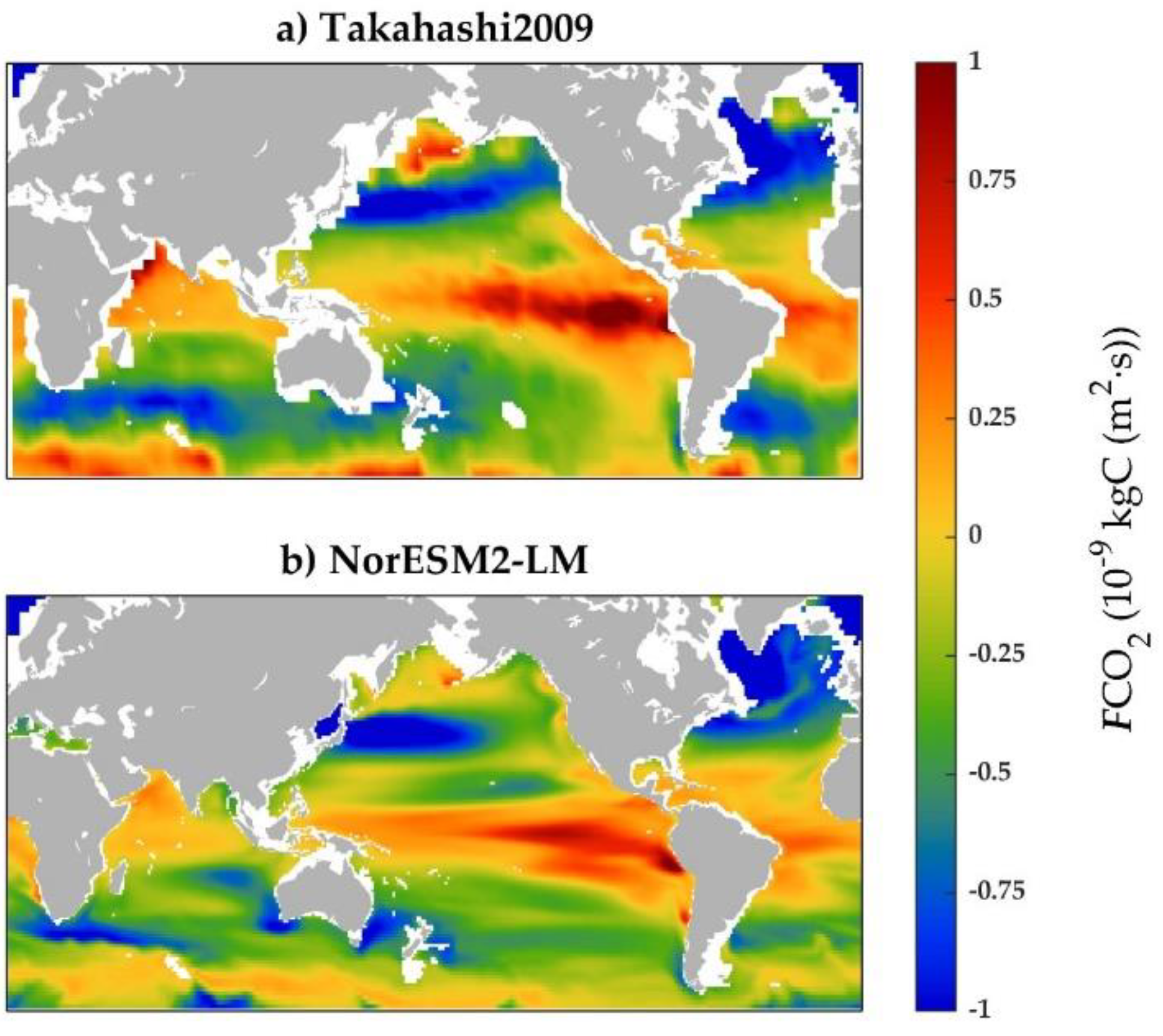
Figure 2.
The time series variations of global-integrated-averaged (a) DIC, (b) pCO2, (c) pH, and (d) Ω for the esm-ssp585 (blue) and esm-ssp585-ocn-alk (orange) experiment conducted by the NorESM2-LM. The details in brackets imply the annual trends of related parameters, respectively. For details, please refer to the Section 3.2.
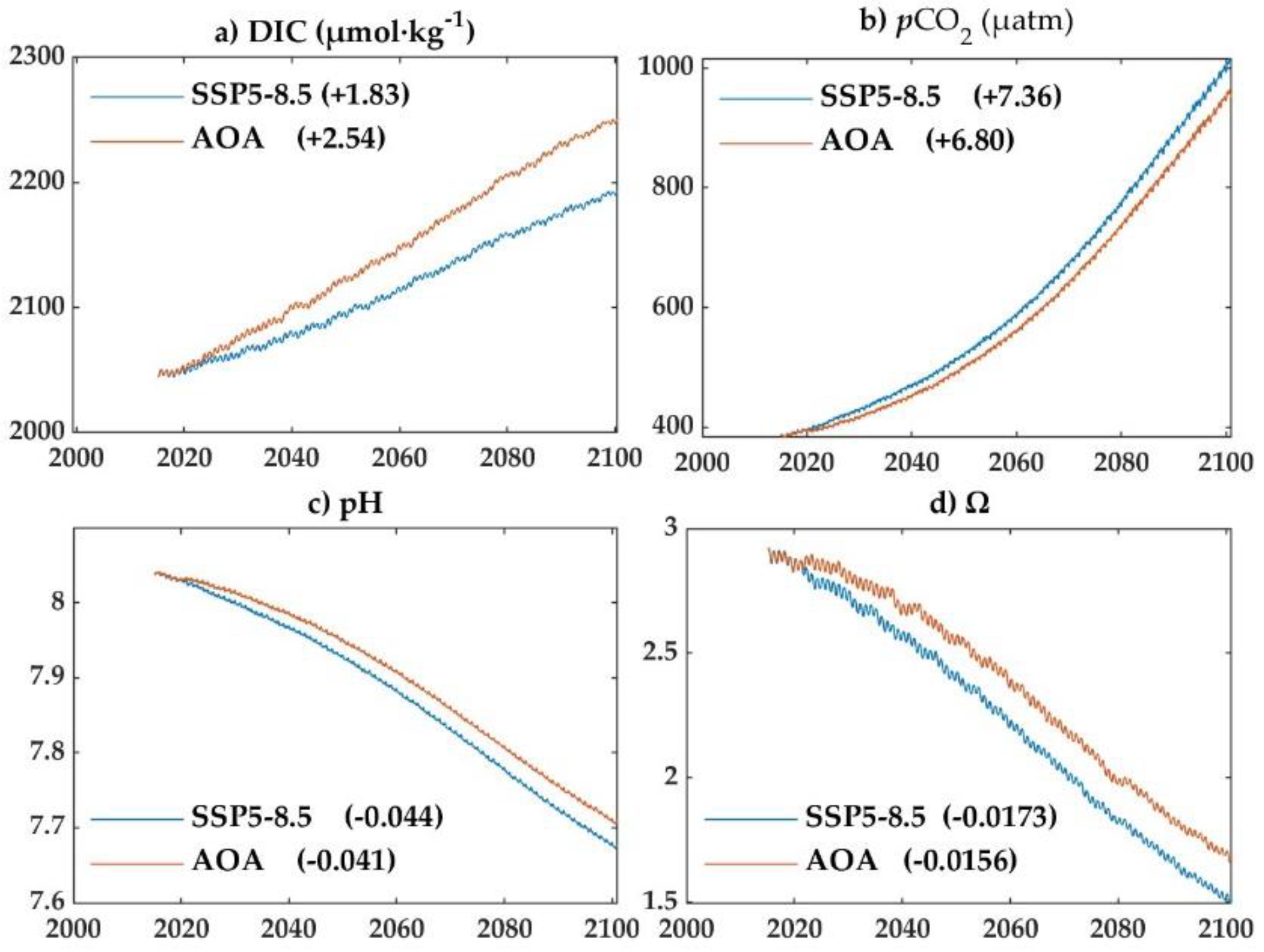
Figure 3.
Changes in surface distributions of (a) DIC, (b) pCO2, (c) pH, and (d) Ω calculated as the average differences between the AOA esm-ssp585-ocn-alk and the no-AOA esm-ssp585.
Figure 3.
Changes in surface distributions of (a) DIC, (b) pCO2, (c) pH, and (d) Ω calculated as the average differences between the AOA esm-ssp585-ocn-alk and the no-AOA esm-ssp585.
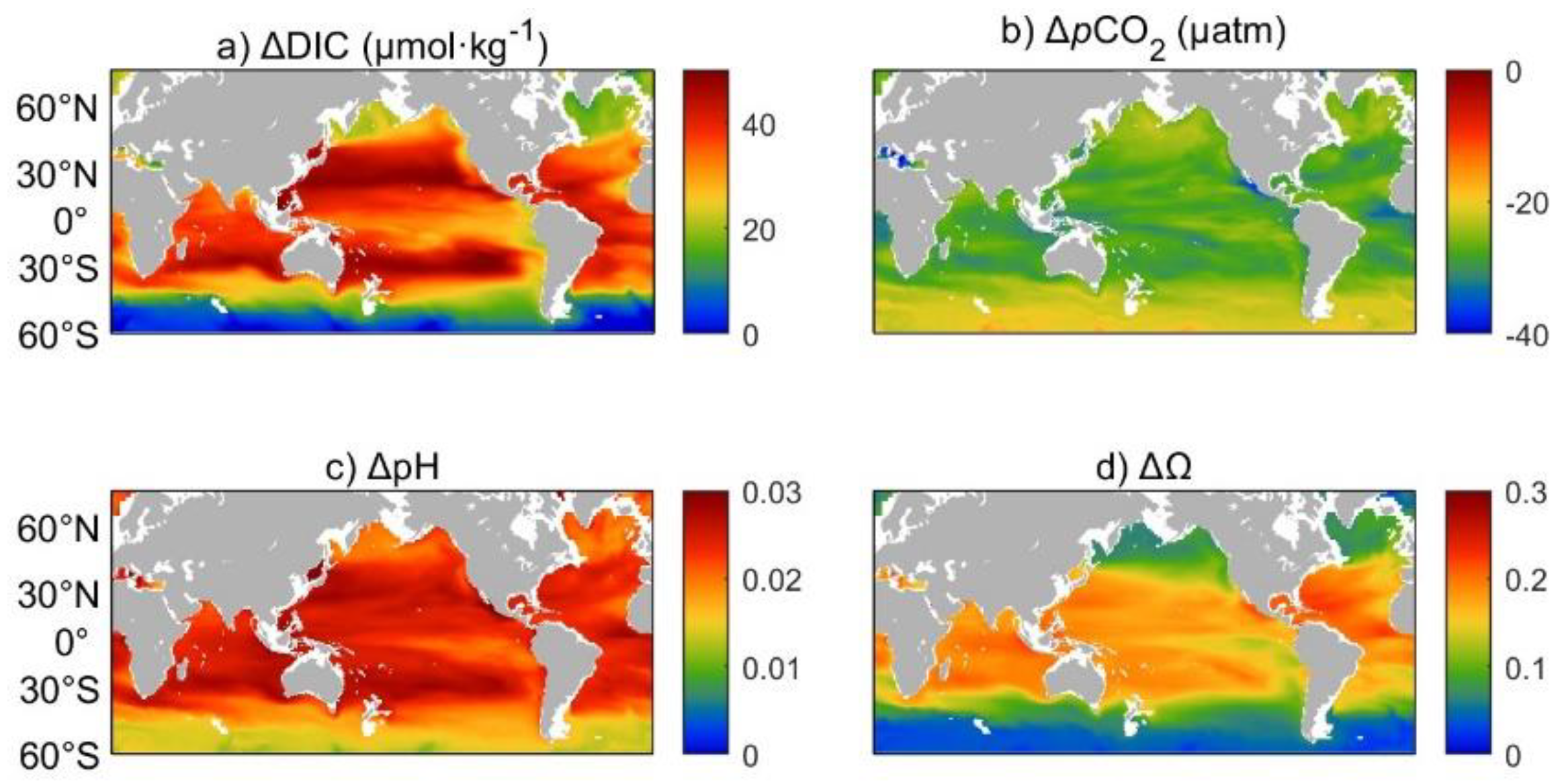
Figure 4.
Annual net global air-sea CO2 exchange flux rates of the no-AOA esm-ssp585 (blue), and the AOA esm-ssp585-ocn-alk (orange). The details in brackets imply the annual trends of related parameters, respectively. For details, please refer to Section 3.3.
Figure 4.
Annual net global air-sea CO2 exchange flux rates of the no-AOA esm-ssp585 (blue), and the AOA esm-ssp585-ocn-alk (orange). The details in brackets imply the annual trends of related parameters, respectively. For details, please refer to Section 3.3.
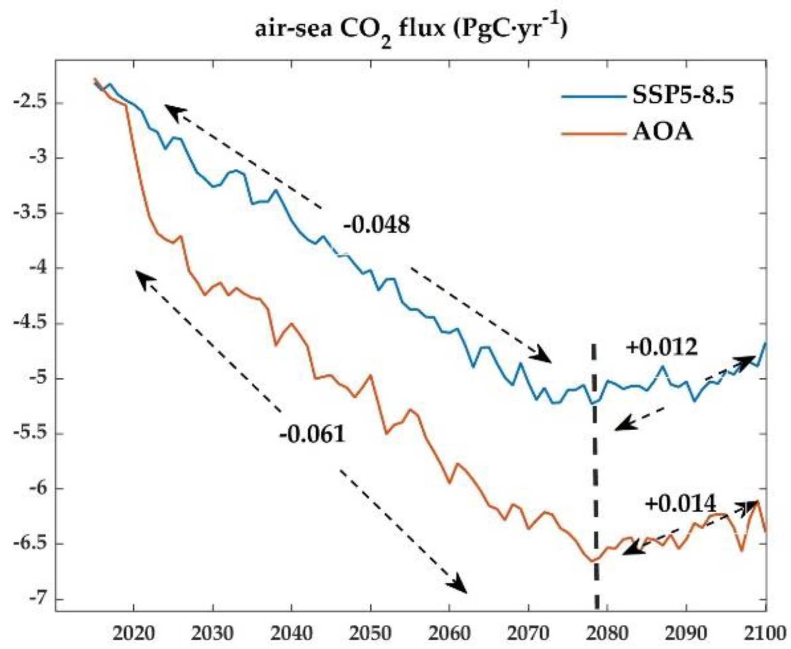
Figure 5.
Globally averaged atmospheric CO2 concentrations of (bule) the no-AOA esm-ssp585, and (orange) the AOA esm-ssp585-ocn-alk. The details in brackets imply the trends of related parameters, respectively. For details, please refer to Section 3.3.
Figure 5.
Globally averaged atmospheric CO2 concentrations of (bule) the no-AOA esm-ssp585, and (orange) the AOA esm-ssp585-ocn-alk. The details in brackets imply the trends of related parameters, respectively. For details, please refer to Section 3.3.
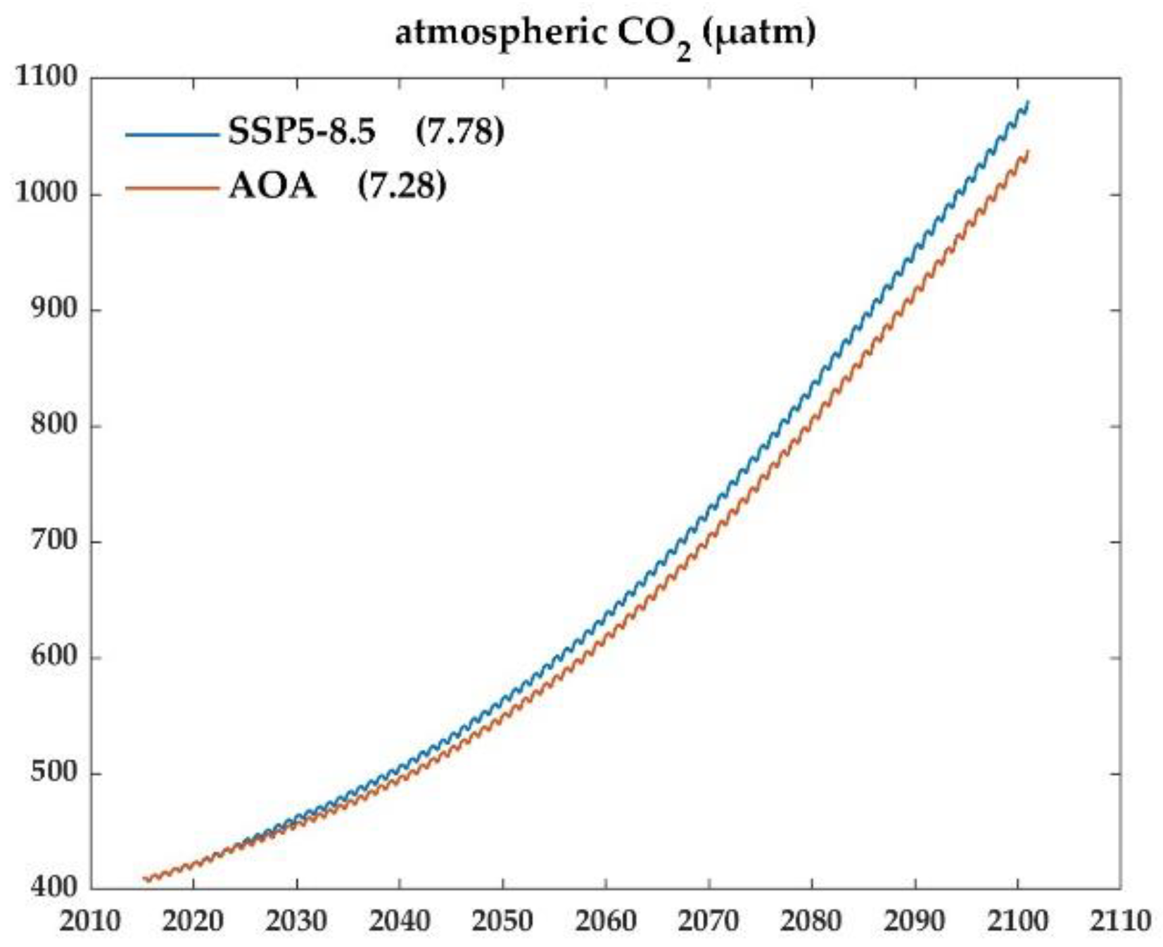
Figure 6.
Globally averaged aragonite saturation depth (bule) the no-AOA esm-ssp585, and (orange) the AOA esm-ssp585-ocn-alk. The details in brackets imply the annual trends of related parameters, respectively. For details, please refer to Section 3.4.
Figure 6.
Globally averaged aragonite saturation depth (bule) the no-AOA esm-ssp585, and (orange) the AOA esm-ssp585-ocn-alk. The details in brackets imply the annual trends of related parameters, respectively. For details, please refer to Section 3.4.
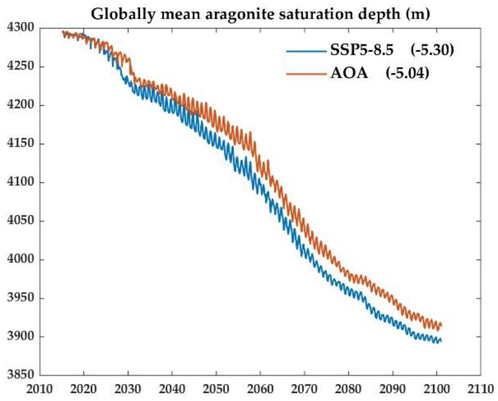

Table 1.
Ocean alkalinization experiment simulations conducted by the NorESM2-LM.
| CMIP6 Experiment ID | Simulation description | Run time |
|---|---|---|
| esm-his | CO2-emission-driven historical scenario | 1850-2014 |
| esm-ssp585 | CO2-emission-driven SSP5-8.5 scenario | 2015-2100 |
| esm-ssp585-ocn-alk | SSP5-8.5 scenario with 0.14 Pmol yr−1 alkalinity added | 2015-2100 |
Disclaimer/Publisher’s Note: The statements, opinions and data contained in all publications are solely those of the individual author(s) and contributor(s) and not of MDPI and/or the editor(s). MDPI and/or the editor(s) disclaim responsibility for any injury to people or property resulting from any ideas, methods, instructions or products referred to in the content. |
© 2025 by the authors. Licensee MDPI, Basel, Switzerland. This article is an open access article distributed under the terms and conditions of the Creative Commons Attribution (CC BY) license (http://creativecommons.org/licenses/by/4.0/).
Copyright: This open access article is published under a Creative Commons CC BY 4.0 license, which permit the free download, distribution, and reuse, provided that the author and preprint are cited in any reuse.


