Submitted:
20 March 2025
Posted:
20 March 2025
You are already at the latest version
Abstract
Global water demand due to population growth and agricultural development, has led to widespread overexploitation of groundwater, particularly in semi-arid regions. Traditional hydrochemistry monitoring system still suffers from limited laboratory accessibility and high costs. This study aims to predict major ions of groundwater, including Ca²⁺, Mg²⁺, Na⁺, SO₄²⁻, Cl⁻, K⁺, HCO₃⁻, and NO₃⁻, utilizing two field measurable parameters (i.e., total dissolved solids (TDS) and mineralization (MIN)) in Aflou_Syncline region, Algeria. A multilayer perceptron (MLP) model optimized with the Levenberg-Marquardt backpropagation (LMBP) provided the most predictive accuracy for the different ions of SO₄²⁻, Mg²⁺, Na⁺, Ca²⁺, and Cl⁻ with R2 = (0.842, 0.980, 0.759, 0.945, 0.895) and RMSE = (53.660, 12.840, 14.960, 36.460, 30.530) (mg/L) in the testing phase, respectively. However, the predictive accuracy for the remaining ions of K⁺, HCO₃⁻, and NO₃⁻ was supplied as R² = (0.045, 0.366, 0.004) and RMSE = (6.480, 41.720, 40.460) (mg/L), respectively. The performance of our model (LMBP-MLP) was validated in similar geological areas in the adjacent area, including Aflou, Madna, and Ain Madhi. In addition, LMBP-MLP showed very promising results, with performance similar to the original research area.
Keywords:
Groundwater ions
; artificial neural networks
; groundwater overexploitation
; semi-arid regions
; hydrochemical monitoring
1. Introduction
Global demand for water is expected to surge by 2050 due to population growth, economic growth, and changing consumption patterns. Estimates suggest that as many as 6 billion people could face water shortages if demand increases by 20 to 30 percent from current levels [1]. Agriculture, which accounts for 70% of global freshwater withdrawals, will increase competition for resources, especially in dry areas [2,3]. These challenges were illustrated in Algeria obviously, where groundwater quality, a major source of irrigation in arid regions, is declining due to salinity and agricultural pollution [4,5]. For this reason, groundwater quality monitoring is very important for sustainable water resource management [6,7]. Extensive sampling campaigns and extensive water chemistry scans are required to monitor the amount of degradation. These scans should include the important chemical ions in water such as Ca2⁺, Mg2⁺, Na⁺, K⁺, HCO3⁻, Cl⁻, and SO42⁻ [8,9]. Effective monitoring, however, still requires significant resources and ongoing sampling and analysis. This highlights the urgency of innovative solutions such as artificial neural networks to streamline water quality assessment [10].
Artificial intelligence (AI) has emerged as an innovative tool to simplify water quality assessment. Early application includes [11], who predicted the drinking water quality index (WQI) of Baghdad using artificial neural networks (ANN), identified pH and chloride as the main factors (R2=0.973). Subsequent work by [12] optimized the ANN architecture for prediction, showing that a simpler MLP-4-5-4 model performed better accuracy (R2=0.989) than a deeper network. Based on these foundations, [13] accomplished nitrate concentration predictions by integrating land use data with pH, conductivity, and temperature, highlighting the adaptability of ANN to multivariable systems. More recently, [9] developed an ANN to predict ion concentrations (Ca2⁺, Mg2⁺, Na⁺, K⁺, HCO3⁻, Cl⁻, and SO42⁻) directly from electrical conductivity (EC), achieving high accuracy within the trained EC range. These developments are consistent with a broader trend in ANN-based environmental modeling, with hybrid approaches combining physical and data-driven models gaining popularity.
These methodological innovations have been applied to address regional challenges. [14] compared radial basis function neural networks (RBF-NN) and probabilistic neural networks (PNN) in Iraq’s Alnekheeb Basin. They found that PNN was superior in assessing irrigation suitability through salinity and sodium uptake ratios. Similarly, [15] utilized ANN to predict groundwater salinity, outperforming conventional regression models and enabling tailored irrigation strategies for salinity-sensitive crops in Spain’s Campo de Cartagena. Furthermore, [16] demonstrated the scalability of ANN in stressed groundwater layers, achieving perfect TDS prediction (R2=0.984) in the Babylonian region of Iraq. However, there are still gaps in applying these technologies to regions with complex evaporite geology, such as the semi-arid regions of North Africa.
In this research, the authors focused on the application of ANN techniques in the Aflou_syncline region of Algeria, a region with distinct geological and climatic features and dependent on groundwater stored in sandstone strata influenced by Aptian gypsum and Triassic evaporite [17]. Here, the increase in the number of wells and the intensive exploitation of groundwater resources have accelerated evaporation and dissolution, increasing the risk of salinity [4]. This research attempted to estimate the ions including Ca2⁺, Mg2⁺, Na⁺, K⁺, SO42⁻, Cl⁻, NO3⁻, and HCO3⁻ employing ANN optimized with various learning algorithms based on two field measured parameters including total dissolved solids (TDS) and mineralization (MIN) values.
The progress of this research is structured as follows. Chapter 2 explains research material including study area and data collection. Chapter 3 presents model and evaluation including artificial neural networks, optimization algorithm, and measures of accuracy. Chapter 4 provides methodology including model development and hyperparameters selection. Chapter 5 organizes the results and discussion including testing the developed model in adjacent areas. Finally, the main conclusions are addressed in Chapter 6.
2. Research Material
2.1. Subsection Study Area and Data Collection
The objective of this study was to predict major ion concentrations, including Ca2+, Mg2+, Na+, K+, SO42⁻, Cl⁻, NO3⁻, and HCO3⁻, utilizing two field-measured parameters, total dissolved solids (TDS) and mineralization (MIN) in the Barremian-Aptian-Albian groundwater system of Aflou_Syncline region. Situated in the Central Sahara Atlas, about 300 km southwest of Algiers, Aflou_Syncline region is located north of Djebel Amour, at 1,400 m above sea level (Figure 1).
From its geographical coordinates (i.e., 34.11°N and 2.10°E), it is located in a mountainous area that acts as a natural barrier between the Sahara Atlas and the Sahara Plateau. This high terrain further exacerbates the climatic contrasts, protecting the region from Mediterranean influences and creating a semi-arid climate with relatively cool temperatures and limited rainfall. Geologically, the area is part of the Saharan Atlas Fold Belt, composing of Mesozoic sediments that date from the Triassic to the Cretaceous. These deposits reflect alternating marine and continental deposits, with limestone, limestone-rich beds, and sandstone-dominated strata. To accomplish this research, 153 groundwater samples were collected from wells distributed throughout the research area and analyzed at the National Office of Water Resources (NAWR) Hydrology Laboratory. These datasets form the basis for modeling correlation among total dissolved solids (TDS), mineralization (MIN), and major ion concentrations employing ANN.
For this purpose, the dataset was split into three subsets: training (75%), validation (15%), and test (10%). The training subset was utilized to adjust the model parameters, while the validation subset was utilized for fine-tuning hyperparameters and mitigate overfitting. Finally, the test subset was utilized to assess the model’s generalization capability, evaluating its performance on new data.
3. Model and Evaluation
3.1. Artificial Neural Networks and Optimization Algorithms
A multilayer perceptron (MLP), also known as a feedforward connected neural networks (FCNN), is a fundamental architecture in deep learning in which every neuron in one layer is connected to all neurons in the next layer, allowing the network to learn nonlinear and complicated relationships in the data [18].
The training concept of MLP is the process of optimizing weights and biases to minimize the loss function, and is usually accomplished utilizing the backpropagation method, a gradient-based optimization algorithm [19]. Backpropagation applies the chain rule to compute the gradient of the loss function for each weight, allowing the network to iteratively adjust its parameters [20]. However, standard backpropagation can be slow to converge or unstable, which has led to the development of advanced optimization algorithms.
These optimizing algorithms include 1) Levenberg-Marquardt (trainlm), which combines gradient descent and Gauss-Newton methods for fast convergence, but requires significant memory; 2) Conjugate Gradient with Polak-Ribière Updates (traincgp), which is memory efficient and suitable for large networks; 3) Gradient Descent with Momentum and Adaptive Learning Rate (traingdx), which utilizes momentum to accelerate convergence and adapts the learning rate dynamically; 4) One-Step Secant (trainoss), which approximates the Hessian matrix to reduce computational complexity; 5) BFGS Quasi-Newton (trainbfg), a second-order optimization method that approximates the inverse Hessian for faster convergence; 6) Conjugate Gradient with Powell-Beale Restarts (traincgb), which periodically resets the search direction to avoid stagnation; 7) Gradient Descent with Adaptive Learning Rate (traingda), which adjusts the learning rate based on gradient behavior; 8) Resilient Backpropagation (trainrp), which updates weights based on the sign of the gradient rather than its magnitude, making it robust to gradient vanishing; and 9) Conjugate Gradient with Fletcher-Reeves updates (traincgf), another conjugate gradient method, ensures efficient optimization [21,22,23,24,25].
The addressed optimization algorithms are implemented in various machine learning frameworks, such as MATLAB’s neural network toolbox, and are chosen based on problem requirements, including network size, data complexity, and computational constraints. For example, Levenberg-Marquardt (trainlm) algorithm is often utilized for small to medium-sized networks because of its speed, whereas Conjugate Gradient with Polak-Ribière Updates (traincgp) and Conjugate Gradient with Powell-Beale Restarts (traincgb) algorithms are preferred for large networks because of their memory efficiency. Also, the choice of optimization algorithm depends on the characteristics of loss surface. In addition, BFGS Quasi-Newton (trainbfg), one of second-order methods is effective on smooth, convex surfaces, whereas Gradient Descent with Momentum and Adaptive Learning Rate (traingdx), a first-order method, is more versatile on non-convex terrain [23,26,27].
3.2. Measures of Accuracy
To evaluate the performance of developed model, the authors employed two main statistical measures of accuracy, namely the coefficient of determination (R2) (Eq. 1) and the root mean square error (RMSE) (Eq. 2). R2 quantifies the proportion of variance in the dependent variable that can be predicted by the independent variables, providing insight into the explanatory power of developed model. Also, it assesses the predictive accuracy by comparing the model’s performance to the mean of the measured data, with values closer to one indicating a better fit [7,28]. In addition, RMSE provides a simple way to interpret a predictive accuracy by measuring the average size of the error between the predicted and measured values [29,30].
(1)
(2)
Where, = The predicted values, = The measured values,
= The mean of the measured values, = The mean of the predicted values, n = The number of data available.
In addition, the authors incorporated ion balance (a chemical index) to assess the model’s predictive ability to maintain chemical balance, which is especially important for applications involving water quality or environmental chemistry. Also, the addressed measurements provide a comprehensive assessment of the model’s predictive accuracy and reliability.
Ionic equilibrium is often evaluated via the charge balance (CB) index (Eq. 3), which is an important metric for assessing chemical consistency of a solution, especially in water quality researches [31]. The interpretation of charge balance values depends on specific thresholds defined for the analysis context such as Eq.4 and Eq. 5.
(3)
(4)
(5)
Where, ΣC = sum of cations (mg/L) and ΣA = sum of anions (mg/L).
For instance, a |CB| value of less than 5 indicates a good ionic balance, reflecting a high degree of chemical consistency. A |CB| between 5 and 8 suggests a moderate ionic balance, while a |CB| greater than 8 signifies a poor ionic balance, indicating potential issues with the chemical composition. However, these thresholds can vary depending on the research’s requirements. In other cases, |CB|<6 may be considered good, 6≤|CB|≤12 is moderate, and |CB|>12 is poor. For more lenient assessments, thresholds such as |CB|<10 (good), 10≤|CB|≤20 (moderate), and |CB|>20 (poor) might be applied. These ranges help to classify the reliability of ion balances, ensuring the accuracy and validity of chemical data in environmental or analytical studies [32].
4. Methodology
4.1. Model Development
In this research, a Levenberg-Marquardt backpropagation multilayer perceptron (LMBP-MLP) was trained to predict the concentrations of important ions (i.e., Ca2⁺, Mg2⁺, Na⁺, SO42⁻, Cl⁻, K⁺, HCO3⁻, and NO3⁻) in water utilizing measurements of MIN, TDS, and some ions (i.e., Mg2⁺, Na⁺, and SO42⁻). The selection of appropriate feature variables and hyperparameters, including the number of neurons in the hidden layer, the type of activation function, the type of learning function, and the learning rate of ANN model, played a critical role in the model development.
The selection of appropriate features for each ANN model (LMBP-MLP) was guided by a correlation heatmap of Pearson correlation coefficients, ensuring that the most relevant variables were utilized for each ion prediction (see Figure (2)). A correlation matrix helps to identify factors that exhibit statistical association based on the Pearson correlation coefficient, which quantifies the linear relationship between two variables. Figure 2 demonstrated that MIN and TDS showed strong correlations with most ions, especially SO42⁻, Na⁺, Mg2⁺, Ca2⁺, and Cl⁻, with correlation coefficients exceeding 0.85. This suggested that these elements originated primarily from evaporite deposits, such as gypsum and saltpeter, found in the Triassic and Aptian formations, and from limestone layers embedded within the Baremian-Aptian sandstone formations, which constitute the most important aquifer system in the region. In contrast, the remaining factors showed weak correlations with coefficients less than 0.53. In particular, NO3⁻ and HCO3⁻ displayed low correlation values, reflecting that the two substances have different origins. In addition, Nitrates (NO3⁻) mainly comes from agricultural fertilizers, while bicarbonates (HCO3⁻) is produced by dissolution of calcite, the main mineral matrix of the Barem-Aptian sandstone. Potassium ions (K⁺), derived from the dissolution of the rare mineral sylvin, is present in low concentrations and contribute minimally to MIN and TDS.
The heatmap also highlighted a very strong correlation for (MIN, SO42⁻) and (TDS, SO42⁻) (PCC>0.95), followed by Na⁺ and Mg2⁺, both of which exhibit significant correlations (PCC>0.92) with MIN and TDS. Both Na⁺ and Mg2⁺ displayed important correlations with SO42⁻ (PCC>0.86). Also, a notable correlation was observed between Ca2⁺ and Cl⁻ with MIN and TDS (PCC>0.85). The moderate correlation was provided between SO42⁻ and Cl⁻ (PCC>0.71). In contrast, the remaining ions (i.e., K⁺, HCO3⁻, and NO3⁻) did not display any significant correlations with the other studied elements. Depending on results of this analysis, feature variables suitable for each ANN model were selected as shown in Table 1.
4.2. Hyperparameters Selection
The activation functions utilized in all developed models include the sigmoid activation function in the hidden layer and the linear transfer function in the output layer. The learning rate was set to 0.001 to ensure stable and efficient training. To select the most suitable training algorithm, the authors trained a model with two neurons utilizing the first three variables (i.e., SO42-, Na+, and Mg2) listed in Table 1. The training algorithm illustrating the highest performance criterion was selected for optimization process. In this research, the evaluated training algorithms included trainlm, traincgp, traingdx, trainoss, trainbfg, traincgb, traingda, trainrp, and traincgf, respectively. Figure 3 shows the performance of training algorithms in this research. Results showed that Levenberg-Marquardt (trainlm) algorithm was superior to remaining algorithms and was the recommended choice for this research.
Choosing the number of neurons in the hidden layer is a critical factor in determining the accuracy of model training process. An excessive number of neurons can lead to overfitting, where the model memorizes noise instead of learning meaningful patterns. Conversely, if there are too few neurons, the model’s capacity to capture complex relationships is limited, which can lead to underfitting [33,34,35].
To enhance the performance of each model, the optimal number of neurons in the hidden layer was determined using a trial-and-error approach, with the number of neurons ranging from 1 to 30. Figure 4 illustrates the effect of difference in the number of hidden neurons on model accuracy in the validation phase. This showed how changing the number of hidden neurons affected the model accuracy. Based on the results, the optimal number of hidden neurons for each model was identified as follows: five neurons for LMBP-MLP1, LMBP-MLP2, and LMBP-MLP3; three neurons for LMBP-MLP4; nine neurons for LMBP-MLP5 and LMBP-MLP7; ten neurons for LMBP-MLP6; and eighteen neurons for LMBP-MLP8.
Figure 5 illustrates the flowchart of modeling process. Initially, SO42⁻ concentrations were predicted based on measured TDS and MIN values. Afterwards, Na⁺ and Mg2⁺ concentrations were computed utilizing measured (i.e., TDS and MIN) and predicted (SO42⁻) values. Also, the prediction of Ca2⁺ concentrations incorporated measured (i.e., TDS and MIN) and predicted (i.e., SO42⁻, Na⁺, and Mg2⁺) values. Similarly, Cl⁻ and K⁺ concentrations were predicted utilizing measured TDS and MIN, along with predicted SO42⁻ and Na⁺ values. Finally, NO3⁻ and HCO3⁻ concentrations were calculated based on measured TDS and MIN, integrating with the predicted Mg2⁺ values.
5. Results and Discussion
Table 2 presents the results of developed ANN models for all major ions in the Aflou_Syncline region of Algeria, utilizing the coefficient of determination (R2) and root mean square error (RMSE) as evaluation metrics in training, validation, and test datasets. The predictive accuracy of model performance varied greatly based on different ANN models.
The following ANN models, including LMBP-MLP1, LMBP-MLP2, LMBP-MLP3, LMBP-MLP4, and LMBP-MLP5, presented the accurate performance, as indicated by high R2 values and relatively low RMSE values across all subsets. This implies that addressed models can accurately predict the concentrations of these ions (SO42⁻, Na⁺, Mg2⁺, Cl⁻, and Ca2⁺) in the Aflou_Syncline region. However, the addressed models, including LMBP-MLP6, LMBP-MLP7, and LMBP-MLP8, provided poorer performance. That is, low R2 values and high RMSE values indicated that these models have difficulty capturing the variability of K+, HCO3-, and NO3- ions.
Figure 6 illustrates the comparison between predicted and measured values of all major ions in the testing phase. Utilizing line plots and scatter plots. It provides a comparative assessment of measured and predicted ion concentrations, providing important insights into the hydrochemical dynamics of the region.
For sulfate (SO42⁻), magnesium (Mg2⁺), and sodium (Na⁺) in the testing phase, the line plots for individual ANN models (i.e., LMBP-MLP1, LMBP-MLP2, and LMBP-MLP3) supplied the strong visual agreement between observed and predicted values, highlighting the reliability of LMBP-MLP1, LMBP-MLP2, and LMBP-MLP3. Scatterplots further quantified this alignment, showing strong predictive accuracy with high coefficients of determination (R2 =0.940 for SO42⁻, R2=0.920 for Mg2⁺, and R2=0.910 for Na⁺).
For calcium (Ca2⁺) and chloride (Cl⁻), The analysis results revealed partial model efficacy. The Ca2⁺ line plot is broadly consistent with the measured trend, but the deviations in 70–80 of samples show that it has limited ability to capture regional differences. The Ca2⁺ scatterplot (R2=0.890) confirmed this, suggesting that high concentrations of outliers led to lower accuracy in the higher ranges. Similarly, the Cl⁻ scatterplot tracks the trend adequately, but underestimates the sharp peak at 90–100 of samples, as evidenced by the clustering of scatterplot outliers (R2=0.870) above the regression line. These discrepancies may arise from extreme values or incomplete representation of location-specific geochemical interactions, highlighting the need for targeted fine-tuning to improve prediction performance for these ions.
In contrast to the strong correlations for SO42⁻, Mg2⁺, and Na⁺, some models (i.e., LMBP-MLP6, LMBP-MLP7, and LMBP-MLP8) provided poor performance for the scatterplots of potassium (K⁺), bicarbonate (HCO3⁻), and nitrate (NO3⁻). The K⁺ scatterplot (R2=0.440) showed minimal agreement with the observed data and failed to reproduce the variability. Also, The HCO3⁻ scatterplot (R2=0.330) provided a nearly random dispersion, indicating a fundamental flaw in either variable selection or mechanical assumptions. Although NO3⁻ scatterplot (R2=0.520) supplied a marginal improvement, LMBP-MLP8 systematically underestimated maximum concentrations, due to unaccounted for anthropogenic or biogeochemical influences.
Figure 7 presents the sorted charge balance (CB) values of all samples utilizing the predicted ion concentrations. It displays aligned equilibrium ion values for 153 water samples from the Aflou_Syncline region employing the predicted ion concentrations. This ion balance serves as an indicator of data quality and the accuracy of ion estimation, with values closer to 0 indicating a better match between positive and negative charges. Samples are classified into three groups: “Good” (green), “Moderate” (yellow), and “Poor” (red) based on their deviation from ion balance. Most of the samples (84%) were classified as “Good”, suggesting the overall reliability of data and satisfactory performance of the developed models. However, 11% of the samples fell into the “Moderate” category, indicating potential problems such as measurement errors, the presence of uncounted ions, or sample degradation. A small number of samples (5%) were classified as “Poor,” indicating serious errors that required reevaluation.
5.1. Testing the Developed Model in Adjacent Areas
To evaluate the generalized ability of developed models, their performance was tested utilizing 20 water samples collected from three external locations within the research area. These locations share the same geological structure as the main research area, but show some petrological differences. The selected locations include Madna (6 samples), Aflou (4 samples), situated southwest of the Aflou_Syncline, and Ain Madhi (10 samples), situated further south. The predictive accuracy of developed models was assessed utilizing the coefficient of determination (R2), and the results were presented in Figure 8.
Our results presented significant differences in model performance across different ions and locations, highlighting that both ion-specific behavior and location-specific characteristics have an impact. The applied models showed high prediction accuracies for SO42⁻, Mg2⁺, and Na⁺, and consistently high R2 values at all points, indicating that the relationships between these ions and the feature variables were stable.
For Ca2⁺ and Cl⁻, the applied models performed well in Aflou and Madna, but supplied poor accuracy in Ain Madhi, suggesting location-specific hydro-geochemical factors that influence ion concentrations. In contrast, the applied models performed poorly for NO3⁻ and K⁺, with R2 values close to 0 at three locations. This is likely due to external influences such as agricultural activities (NO3⁻) and local mineral dissolution (K⁺).
The prediction of HCO3⁻ varied significantly, supplying moderate performance at Madna but low accuracy at Aflou and Ain Madhi, indicating that hydro-geochemical control may be possible depending on the location. The differences of performance in applied models can be attributed to differences in rock composition, groundwater flow dynamics, and local environmental factors affecting ion concentrations.
The geological characteristics at Ain Madhi may provide more pronounced variations than those of Aflou and Madna, which may lead to inconsistencies that the applied models may not fully capture. In addition, location-specific geochemical processes, anthropogenic influences (e.g., fertilizer use affecting NO3⁻), and varying mineral dissolution rates (e.g., sylvite dissolution for K⁺) may contribute to the observed discrepancies.
Overall, the applied models demonstrated strong predictive ability for SO42⁻, Mg2⁺, and Na⁺, whereas it performed poorly for Ca2⁺, Cl⁻, HCO3⁻, NO3⁻, and K⁺, especially at Ain Madhi. These results highlighted the need for additional location-specific calibrations to improve model accuracy for specific ions and account for local hydro-geochemical variations.
To estimate the charge balance (CB) in the adjacent areas of Aflou, Madna, and Ain Madhi, the authors utilized Figure 8 to identify ions with high predictive performance (R2>0.600) and replaced ions with low performance utilizing measured data to ensure accuracy.
The values of selected ions utilized for Ionic Balance calculations varied depending on locations. In Aflou, the selected ions were SO42⁻, Cl⁻, Ca2⁺, Mg2⁺, Na⁺, and K⁺. For Ain Madhi, only SO42⁻, Ca2⁺, Mg2⁺, and Na⁺ satisfied the selection criteria, while in Madna, the chosen ions included SO42⁻, HCO3⁻, Cl⁻, Ca2⁺, Mg2⁺, and Na⁺. The results of the Ionic Balance and their evaluation are presented in Table 3, Table 4, and Table 5.
Each table (Table 3, Table 4, and Table 5) provides predicted and measured ion concentrations, the calculated charge balance, and their evaluation of samples. In Aflou, 75% of the samples were rated as “Good”, indicating reliable data and accurate ion estimates, 25% were rated as “Moderate” and 0% were rated as “Poor”. In contrast, Ain Madhi featured a wider range of sample quality, featuring 50% “Good” samples, along with 30% “Poor” and 20% “Moderate” ratings. This suggests potential data quality issues specific to Ain Madhi, which could arise from sample contamination or measurement errors. Madna, similar to Aflou, gave mostly “Good” ratings (66.67%), with 33.33% being “Moderate” samples, suggesting generally reliable data with localized discrepancies. The variability in charge balance across all regions highlights the importance of ion balance analysis as a tool to assess data quality and validate ion estimates. The presence of “Poor” and “Moderate” samples highlights the need for further investigation to identify and correct potential problems to ensure the accuracy and reliability of hydrochemical data.
6. Conclusion
In Algeria, groundwater remains critical for irrigation, but groundwater quality in areas such as the Aflou region is increasingly compromised by salinity and agricultural contamination, threatening agricultural sustainability. Conventional monitoring methods that rely on expensive sampling campaigns and laboratory analyses highlight the urgent need for innovative and cost-effective solutions to ensure water security. Artificial intelligence (AI), especially artificial neural networks (ANN), has emerged as a revolutionary tool in the field of hydrochemistry.
In this research, the authors introduced a novel algorithm to predict eight major ions (Ca2⁺, Mg2⁺, Na⁺, K⁺, HCO3⁻, SO42⁻, Cl⁻, and NO3⁻) utilizing only two accessible parameters (i.e., total dissolved solids (TDS) and mineralization (MIN). The Levenberg-Marquardt backpropagation multilayer perceptron (LMBP-MLP) model with ion-specific customized architecture achieved robust predictive accuracies for SO42⁻, Mg2⁺, Na⁺, Ca2⁺, and Cl⁻ (R2 and NSE≥0.87), proving its usefulness in real-time monitoring. However, predictive accuracies for K⁺, HCO3⁻, and NO3⁻ were less reliable (R2≤0.50), most likely due to complex environmental interactions and low concentrations leading to little statistical significance. The validation via charge balance analysis confirmed strong ionic balance in 95% of predictions, but 5% showed discrepancies requiring improvement.
Spatial tests across three locations (i.e., Aflou, Madena, and Ain Madhi) showed consistent accuracy for SO42⁻, Mg2+, and Na⁺, moderate performance for Ca2⁺ and Cl⁻, variable results for K⁺ and HCO3⁻, and overall poor prediction of NO3⁻. These results highlighted the model’s adaptability to regions such as Aflou and Madna, while also emphasizing the need for expanded geographic data to improve generalization. Despite these limitations, this algorithm has made great strides in water resource management in salinity-affected areas. Direct TDS and MIN measurements enable early detection of important ions (Ca2⁺, Mg2⁺, Na⁺, SO42⁻, and Cl⁻), providing three key benefits: cost savings, adaptability, and efficiency.
Author Contributions
Conceptualization, S.M.E., A.H.(Abderrahmane Hamimed) and M.Z.; methodology, M.Z.; validation, S.M.E., A.H.(Abderrahmane Hamimed) and S.K.; formal analysis, A.H.(Azzaz Habib)., A.H.(Abderrahmane Hamimed) and M.Z.; investigation, A.H.(Azzaz Habib)., I.C. and S.K.; data curation, S.M.E. and A.H.(Abderrahmane Hamimed).; writing—original draft preparation, S.M.E., A.H.(Azzaz Habib), A.H.(Abderrahmane Hamimed), M.Z., I.C. and S.K.; writing—review and editing, M.Z., I.C. and S.K.; visualization, S.M.E., A.H.(Azzaz Habib) and A.H.(Abderrahmane Hamimed); supervision, S.K.; funding acquisition, I.C. All authors have read and agreed to the published version of the manuscript.
Funding
Research for this paper was carried out under the KICT Research Program (Project No. 20250108-001, Development of IWRM-Korea Technical Convergence Platform Based on Digital New Deal) funded by the Ministry of Science and ICT.
Data Availability Statement
The data presented in this study will be available on interested request from the corresponding author.
Conflicts of Interest
The authors declare no conflicts of interest.
Abbreviations
The following abbreviations are used in this manuscript:
| TDS | Total dissolved solids |
| MIN | Mineralization |
| MLP | Multilayer perceptron |
| LMBP | Levenberg-Marquardt backpropagation |
| AI | Artificial intelligence |
| WQI | Water quality index |
| ANN | Artificial neural networks |
| EC | Electrical conductivity |
| RBF-NN | Radial basis function neural networks |
| PNN | Probabilistic neural networks |
| FCNN | Feedforward connected neural networks |
| R2 | Coefficient of determination |
| RMSE | Root mean square error |
| CB | Charge balance |
| LMBP-MLP | Levenberg-Marquardt backpropagation multilayer perceptron |
References
- UNESCO. The United Nations world water development report 2018. 2019, nature-based solutions for water. UN.
- Boretti, A.; Rosa, L. Reassessing the projections of the world water development report. NPJ Clean Water, 2019, 2, 15. [Google Scholar] [CrossRef]
- Canton, H. Food and agriculture organization of the United Nations—FAO. In The Europa directory of international organizations 2021, 2021, pp. 297-305, Routledge.
- Hamed, Y.; Hadji, R.; Redhaounia, B.; Zighmi, K.; Bâali, F.; El Gayar, A. Climate impact on surface and groundwater in North Africa: a global synthesis of findings and recommendations. Euro-Mediterr. J. Environ. Integr. 2018, 3, 25. [Google Scholar] [CrossRef]
- Bioud, I.; Semar, A.; Laribi, A.; Douaibia, S.; Chabaca, M.N. Assessment of groundwater quality and its suitability for irrigation: the case of Souf Valley phreatic aquifer. Algerian Journal of Environmental Science and Technology.
- Shiri, N.; Shiri, J.; Yaseen, Z.M.; Kim, S.; Chung, I.M.; Nourani, V.; Zounemat-Kermani, M. Development of artificial intelligence models for well groundwater quality simulation: Different modeling scenarios. PLoS One. 2021, 16, e0251510. [Google Scholar] [CrossRef] [PubMed]
- Alizamir, M.; Ahmed, K.O.; Kim, S.; Heddam, S.; Gorgij, A.D.; Chang, S.W. Development of a robust daily soil temperature estimation in semi-arid continental climate using meteorological predictors based on computational intelligent paradigms. PLoS one. 2023, 18, e0293751. [Google Scholar] [CrossRef]
- Lopes, M.B.S. The 2017 World Health Organization classification of tumors of the pituitary gland: a summary. Acta Neuropathol. 2017, 134, 521–535. [Google Scholar] [CrossRef]
- Khadra, F.W.; El Sibai, R.; Khadra, W.M. (2024). Deriving groundwater major ions from electrical conductivity using artificial neural networks supported by analytical hydrochemical solutions. Groundwater Sustainable Dev. 2024, 24, 101056. [Google Scholar] [CrossRef]
- Tao, H. , Hameed, M. M., Marhoon, H.A., Zounemat-Kermani, M., Heddam, S., Kim, S.,... & Yaseen, Z M. Groundwater level prediction using machine learning models: A comprehensive review. Neurocomputing. 2022, 489, 271–308. [Google Scholar]
- Khudair, B.H.; Jasim, M.M.; Alsaqqar, A.S. Artificial neural network model for the prediction of groundwater quality. Civ. Eng. J. 2018, 4, 2959–2970. [Google Scholar] [CrossRef]
- Setshedi, K.J.; Mutingwende, N.; Ngqwala, N.P. The use of artificial neural networks to predict the physicochemical characteristics of water quality in three district municipalities, eastern cape province, South Africa. Int. J. Environ. Res. Public Health. 2021, 18, 5248. [Google Scholar] [CrossRef]
- Stylianoudaki, C.; Trichakis, I.; Karatzas, G.P. Modeling groundwater nitrate contamination using artificial neural networks. Water. 2022, 14, 1173. [Google Scholar] [CrossRef]
- Allawi, M.F.; Al-Ani, Y.; Jalal, A.D.; Ismael, Z.M.; Sherif, M.; El-Shafie, A. Groundwater quality parameters prediction based on data-driven models. Eng. Appl. Comput. Fluid Mech. 2024, 18, 2364749. [Google Scholar]
- Mateo, L.F.; Más-López, M.I.; García-del-Toro, E.M.; García-Salgado, S.; Quijano, M.Á. (2024). Artificial Neural Networks to Predict Electrical Conductivity of Groundwater for Irrigation Management: Case of Campo de Cartagena (Murcia, Spain). Agronomy. 2024, 14, 524. [Google Scholar]
- Al-Sulttani, A.O.; Ali, S.K.; Abdulhameed, A.A.; Jassim, D.T. Artificial Neural Network Assessment of Groundwater Quality for Agricultural Use in Babylon City: An Evaluation of Salinity and Ionic Composition. Int. J. Des. Nat. Ecodyn. 2024, 19, 329–336. [Google Scholar]
- Sekkoum, M.; Safa, A.; Stamboul, M. (2020). Groundwater hydrochemistry of Aflou syncline, Central Saharan Atlas of Algeria. Desalin. Water Treat. 2020, 190, 424–439. [Google Scholar]
- Kim, S.; Cho, J.S.; Park, J.K. Hydrological analysis using the neural networks in the parallel reservoir groups, South Korea. In World Water & Environmental Resources Congress, United States, 2003.
- Kim, S.; Seo, Y.; Lee, C.J. Modeling of rainfall by combining neural computation and wavelet technique. Procedia Eng. 2016, 154, 1231–1236. [Google Scholar]
- Zakhrouf, M.; Bouchelkia, H.; Stamboul, M.; Kim, S.; Heddam, S. Time series forecasting of river flow using an integrated approach of wavelet multi-resolution analysis and evolutionary data-driven models. A case study: Sebaou River (Algeria). Phys. Geogr. 2018, 39, 506–522. [Google Scholar]
- Hagan, M.T.; Demuth, H.B.; Beale, M. Neural network design. PWS Publishing Co, 1997.
- Haykin, S. Neural Networks: A comprehensive foundation. Prentice-Hall Inc. Upper Saddle River, New Jersey, 1999.
- Kim, S.; Lee, S. Forecasting of flood stage using neural networks in the Nakdong river, South Korea. In Watershed Management and Operations Management, United States, 2000.
- Bishop, C.M.; Nasrabadi, N.M. Pattern recognition and machine learning. New York, Springer, 2006.
- Zakhrouf, M.; Bouchelkia, H.; Stamboul, M.; Kim, S.; Singh, V.P. (2020). Implementation on the evolutionary machine learning approaches for streamflow forecasting: case study in the Seybous River, Algeria. J. Korea Water Resour. Assoc. 2020, 53, 395–408. [Google Scholar]
- Rumelhart, D.E.; Hinton, G.E.; Williams, R.J. (1986). Learning representations by back-propagating errors. Nature, 1986, 323, 533–536. [Google Scholar]
- Nocedal, J.; Wright, S.J. Numerical optimization. New York, NY, Springer, 1999.
- Kim, S.; Seo, Y.; Malik, A.; Kim, S.; Heddam, S.; Yaseen, Z.M.; Kisi, O.; Singh, V.P. Quantification of river total phosphorus using integrative artificial intelligence models. Ecol. Indic. 2023, 153, 110437. [Google Scholar]
- Seo, Y.; Kim, S.; Singh, V.P. Physical interpretation of river stage forecasting using soft computing and optimization algorithms. In Harmony Search Algorithm: Proceedings of the 2nd International Conference on Harmony Search Algorithm (ICHSA2015) (pp.
- Alizamir, M.; Gholampour, A.; Kim, S.; Keshtegar, B.; Jung, W.T. Designing a reliable machine learning system for accurately estimating the ultimate condition of FRP-confined concrete. Sci. Rep. 2024, 14, 20466. [Google Scholar]
- Reed, M.H. Calculation of multicomponent chemical equilibria and reaction processes in systems involving minerals, gases and an aqueous phase. Geochim. Cosmochim. Acta. 1982, 46, 513–528. [Google Scholar] [CrossRef]
- Stuyfzand, P.J. Hydrogeochemcal (HGC 2.1), for storage, management, control, correction and interpretation of water quality data in Excel® spread sheet. KWR-rapport B111698-002, 2012.
- Kim, S.; Kim, H.S. Uncertainty reduction of the flood stage forecasting using neural networks model. JAWRA J. Am. Water Resour. Assoc. 2008, 44, 148–165. [Google Scholar] [CrossRef]
- Fushiki, T. Estimation of prediction error by using K-fold cross-validation. Stat. Comput. 2011, 21, 137–146. [Google Scholar] [CrossRef]
- Gu, Y.; Wylie, B.K.; Boyte, S.P.; Picotte, J.; Howard, D.M.; Smith, K.; Nelson, K.J. An optimal sample data usage strategy to minimize overfitting and underfitting effects in regression tree models based on remotely-sensed data. Remote Sens. 2016, 8, 943. [Google Scholar] [CrossRef]
Figure 1.
Geographic map of the research area.
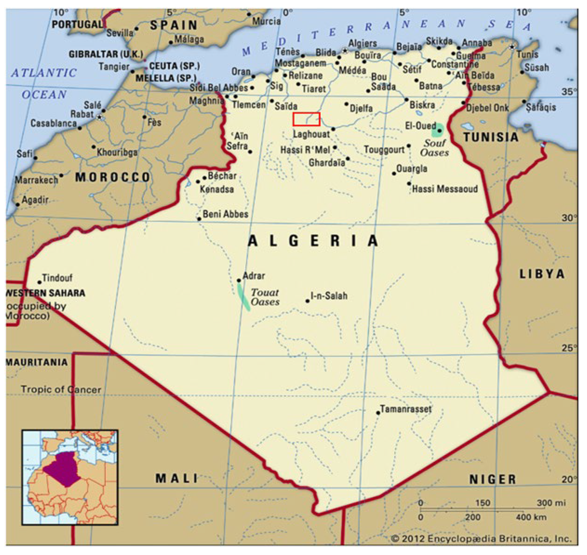
Figure 2.
Heatmap of statistical associations based on the Pearson correlation coefficient (PCC).
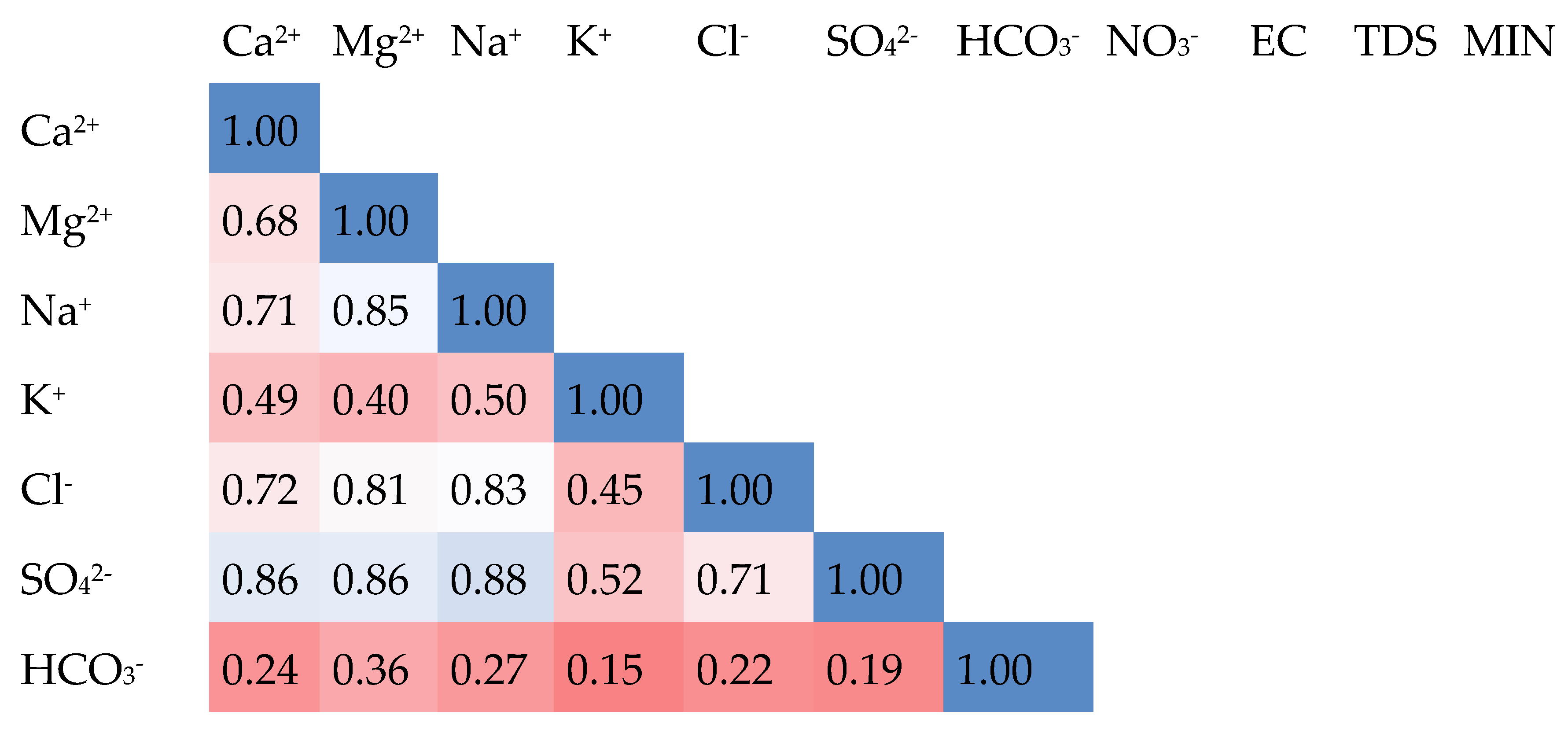
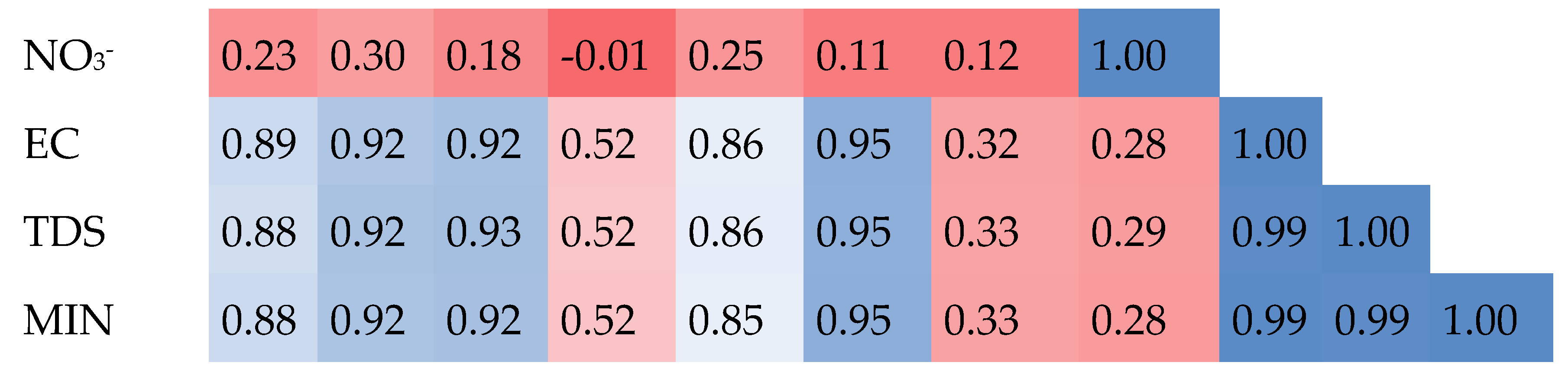
Figure 3.
The performance of training algorithms.
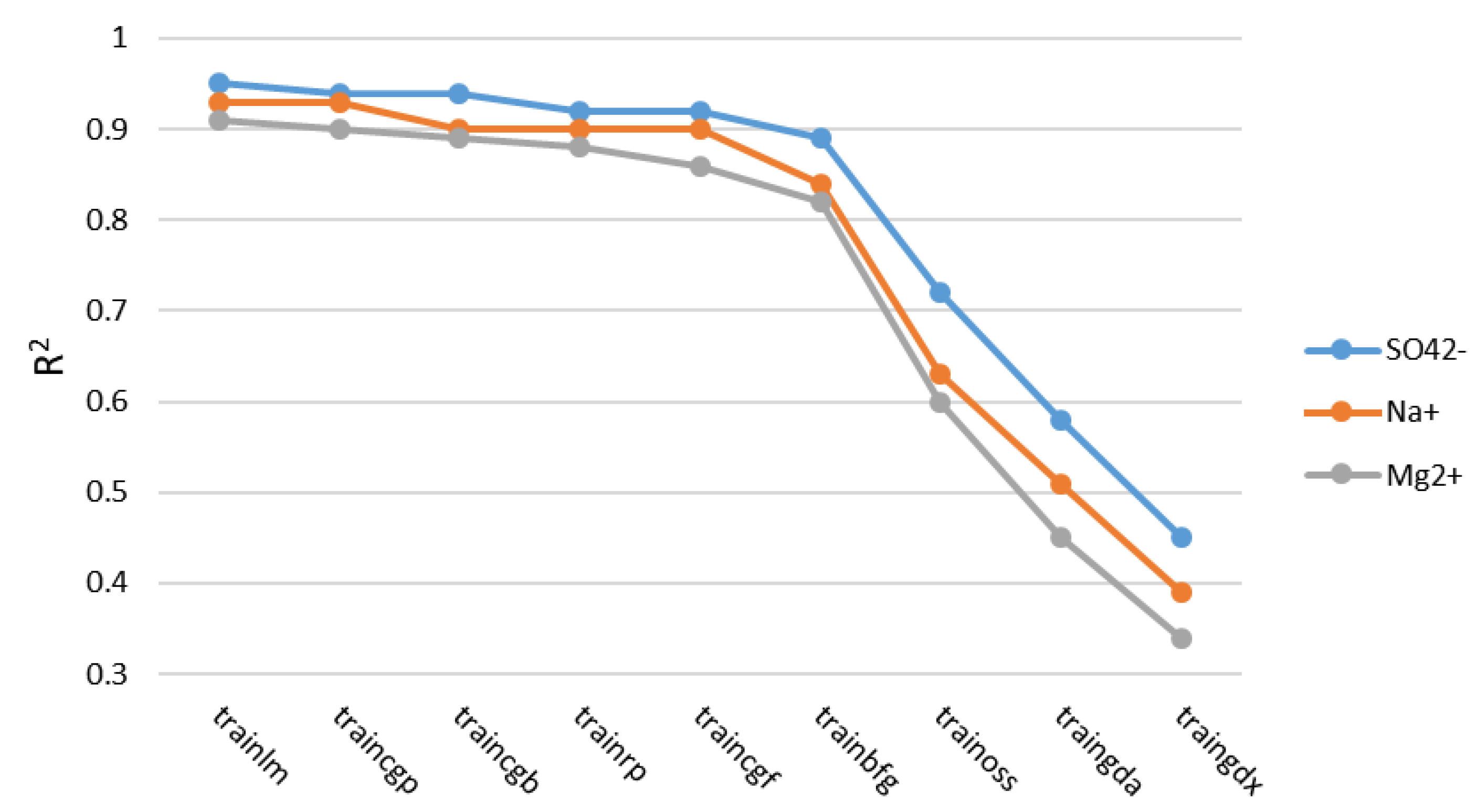
Figure 4.
Effect of the difference in the number of hidden neurons on model accuracy in the validation phase (a) SO42-, (b) Mg2+, (c) Na+, (d) Ca2+, (e) Cl-, (f) K+, (g) HCO3-, and (h) NO3-.
Figure 4.
Effect of the difference in the number of hidden neurons on model accuracy in the validation phase (a) SO42-, (b) Mg2+, (c) Na+, (d) Ca2+, (e) Cl-, (f) K+, (g) HCO3-, and (h) NO3-.
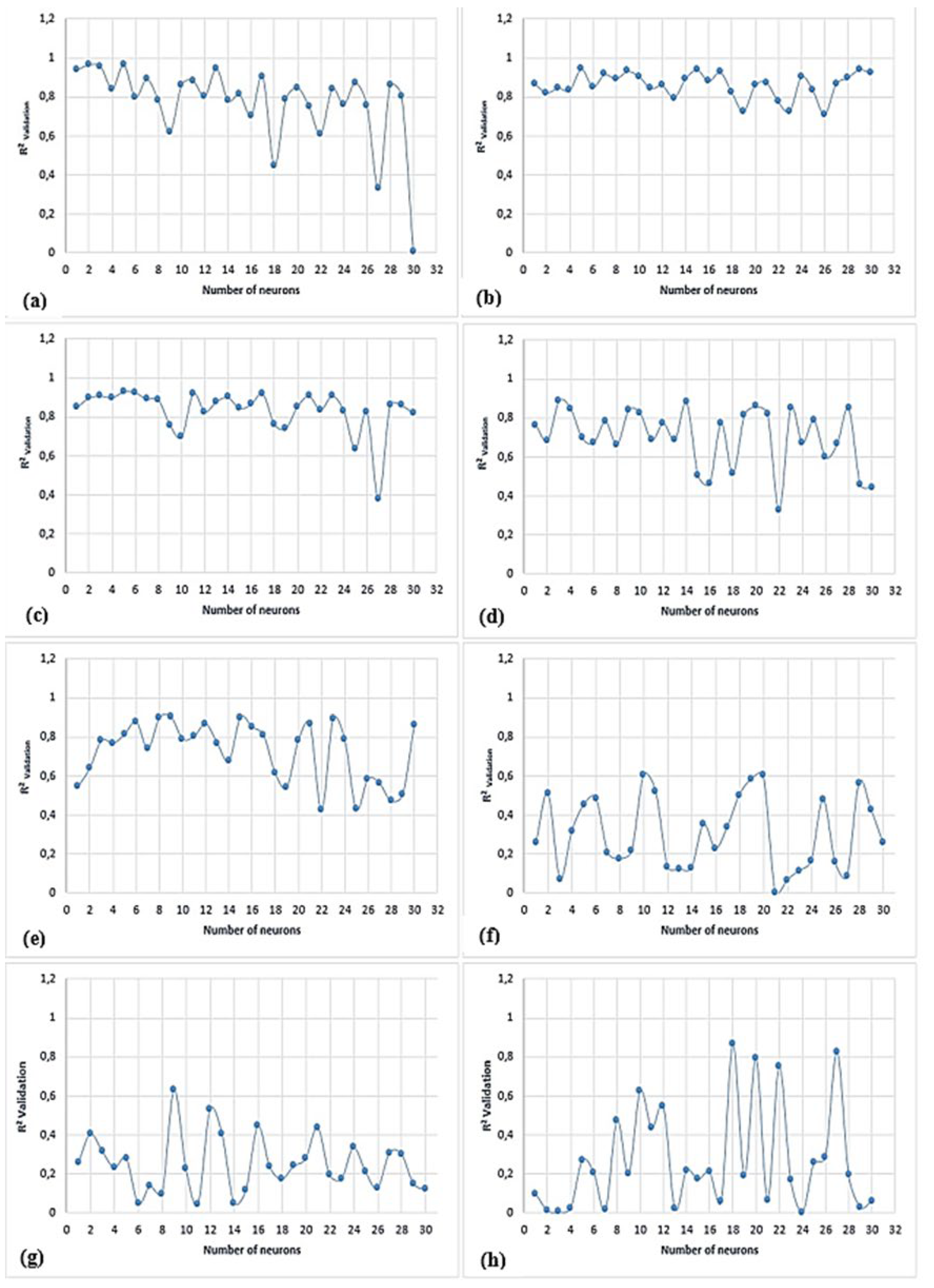
Figure 5.
Flowchart of modeling process.
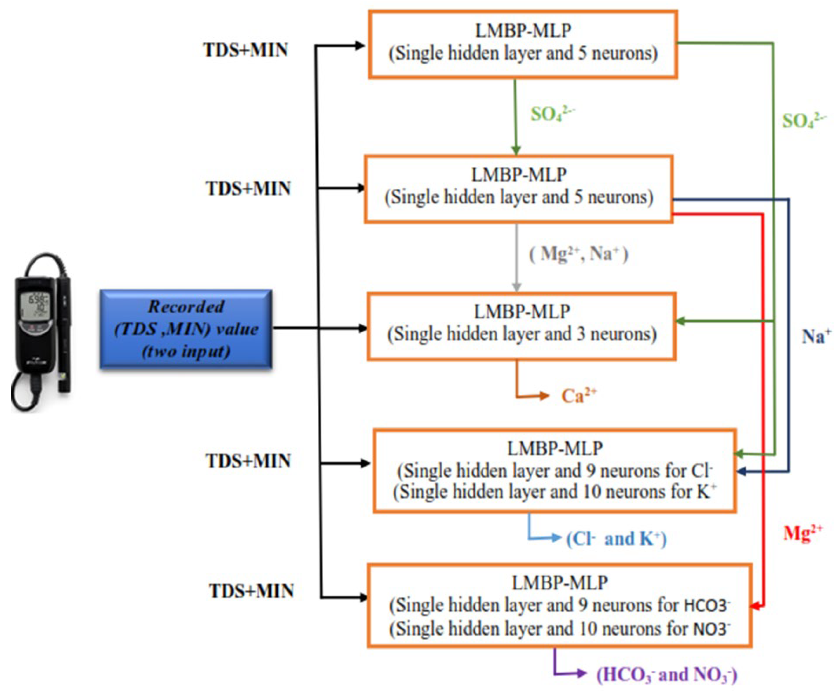
Figure 6.
Comparison between predicted and measured values of all major ions for the all dataset (a) SO42-, (b) Mg2+, (c) Na+, (d) Ca2+, (e) Cl-, (f) K+, (g) HCO3-, and (h) NO3-.
Figure 6.
Comparison between predicted and measured values of all major ions for the all dataset (a) SO42-, (b) Mg2+, (c) Na+, (d) Ca2+, (e) Cl-, (f) K+, (g) HCO3-, and (h) NO3-.
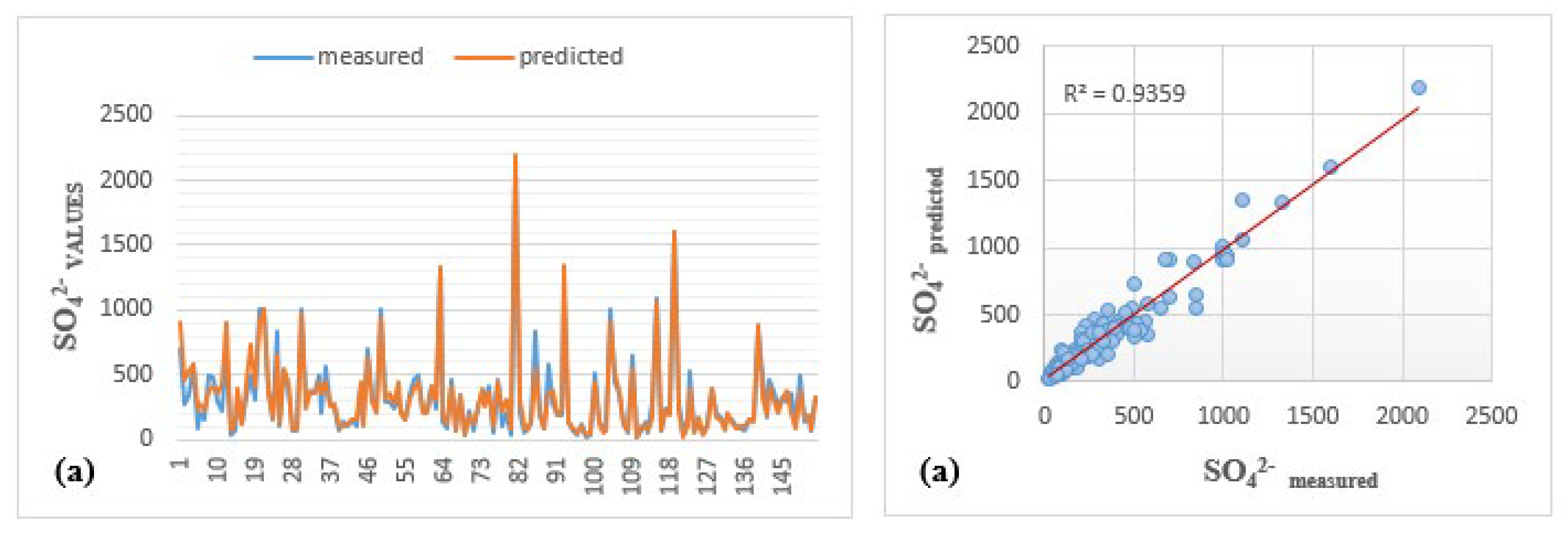
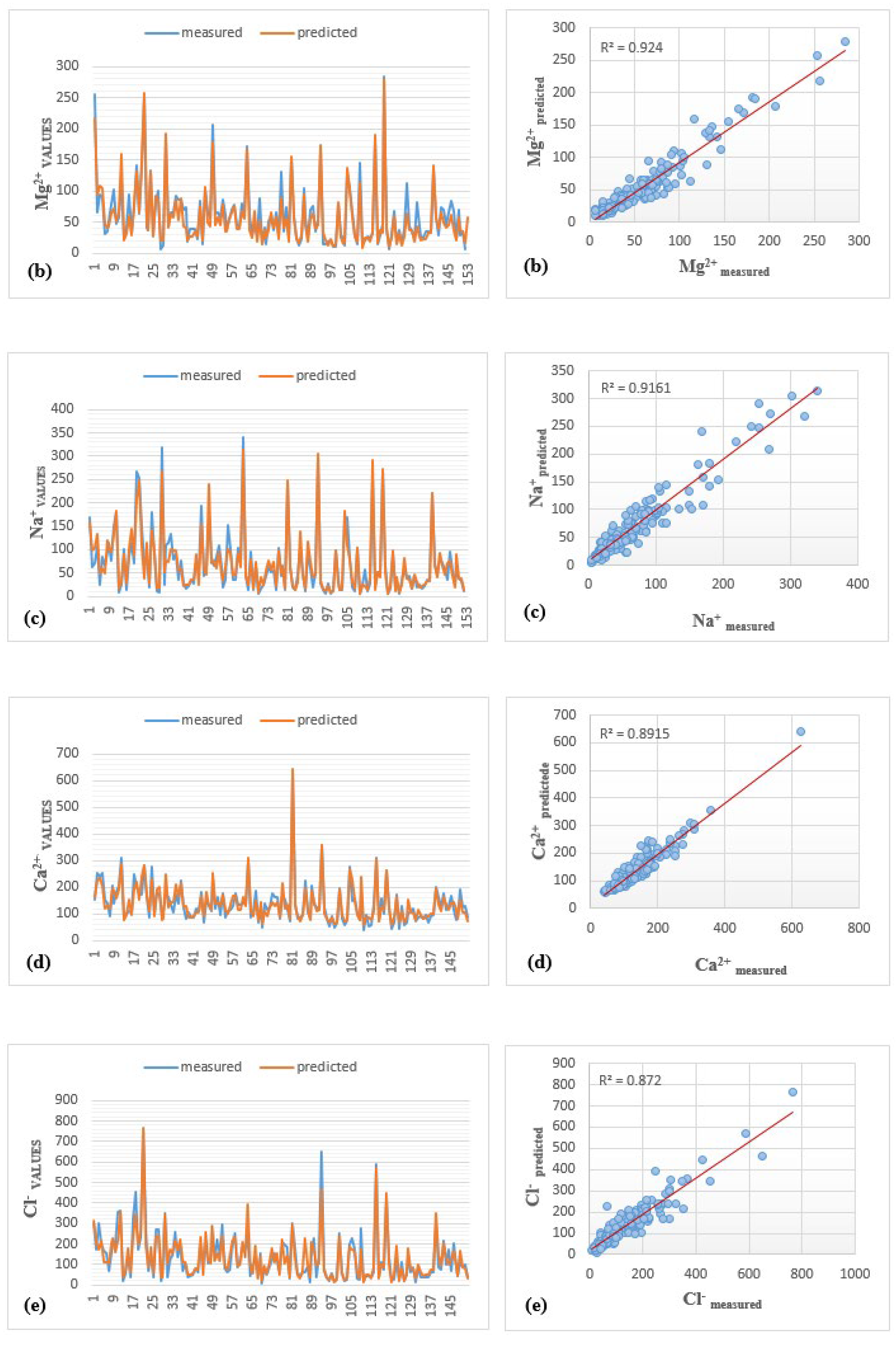
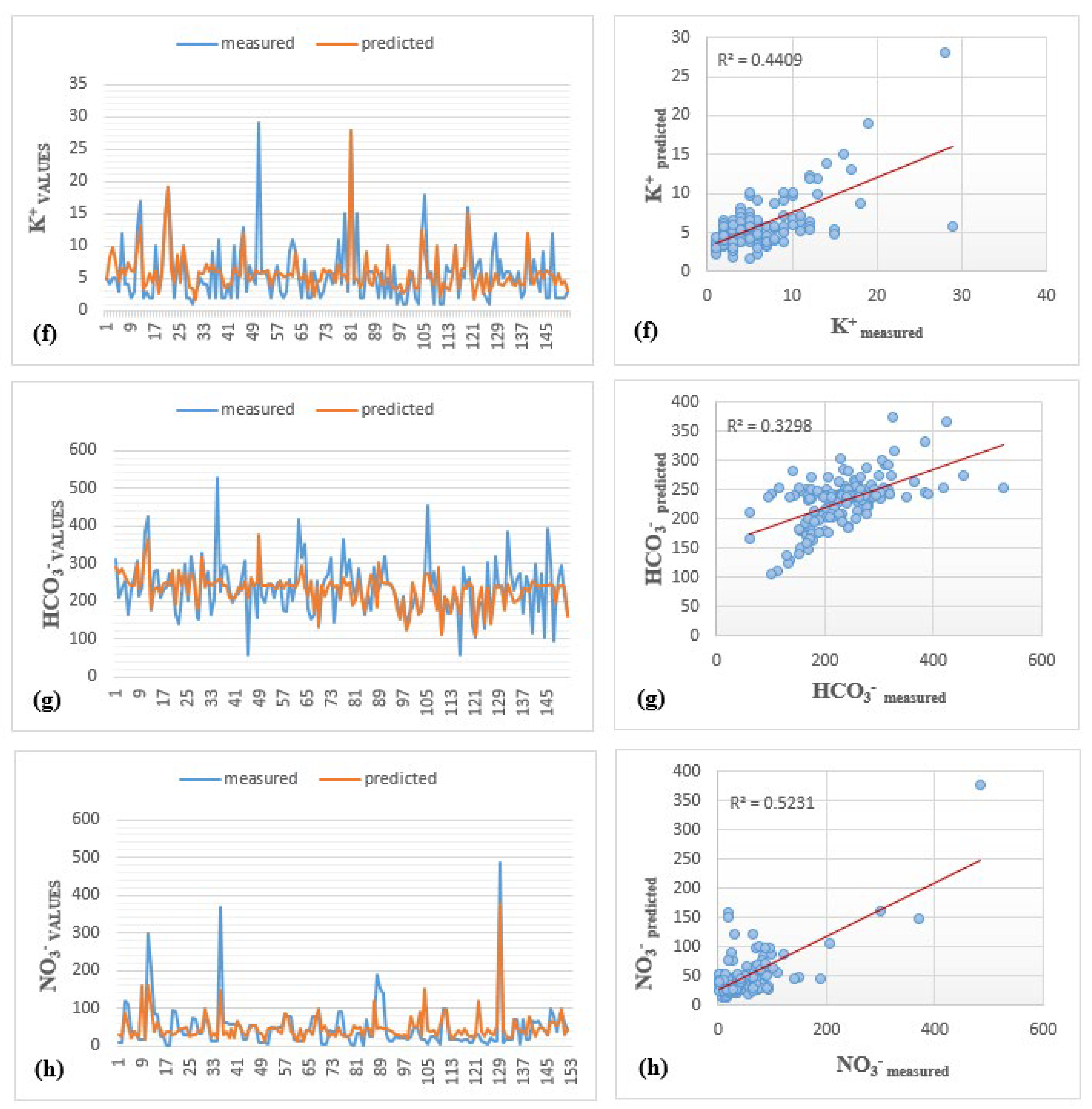
Figure 7.
The sorted charge balance (CB) values of all samples utilizing the predicted ions.
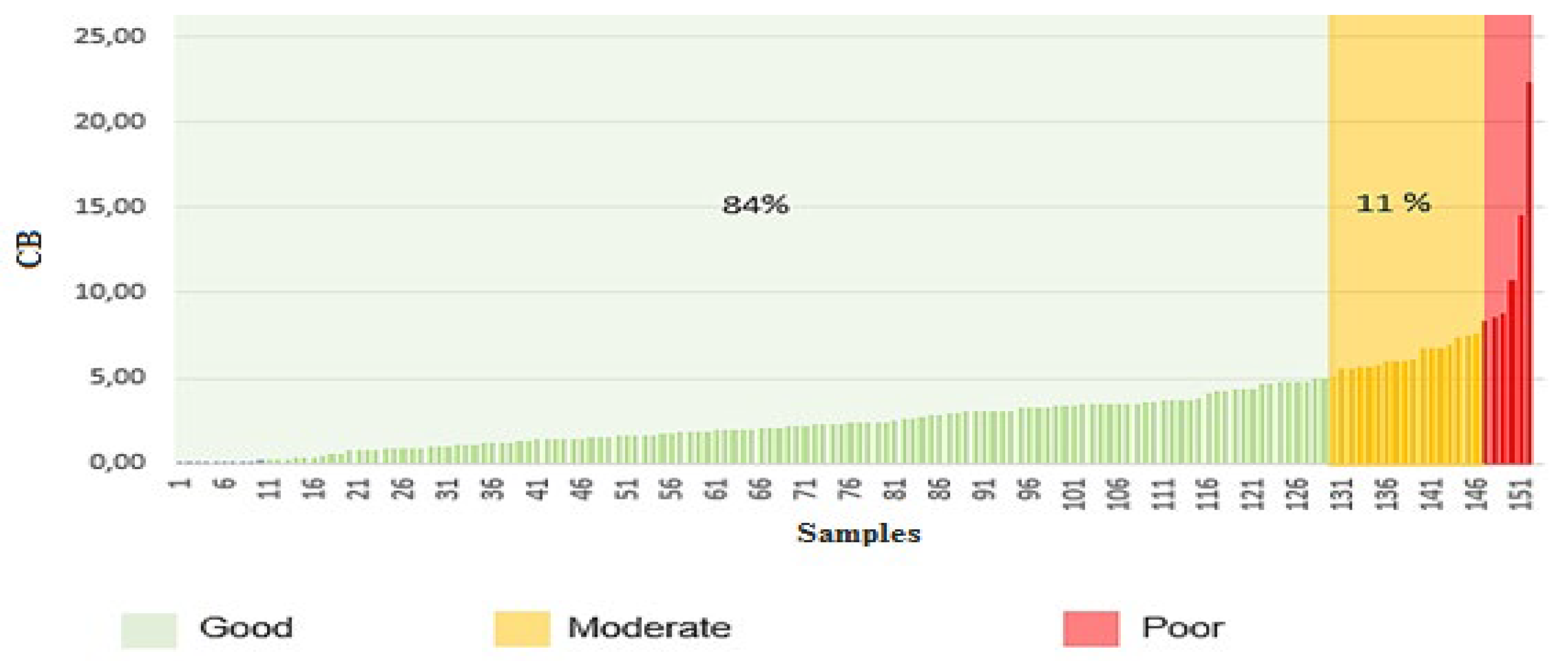
Figure 8.
Comparison of developed models performance in adjacent areas (Aflou, Madena, and Ain Madhi).
Figure 8.
Comparison of developed models performance in adjacent areas (Aflou, Madena, and Ain Madhi).
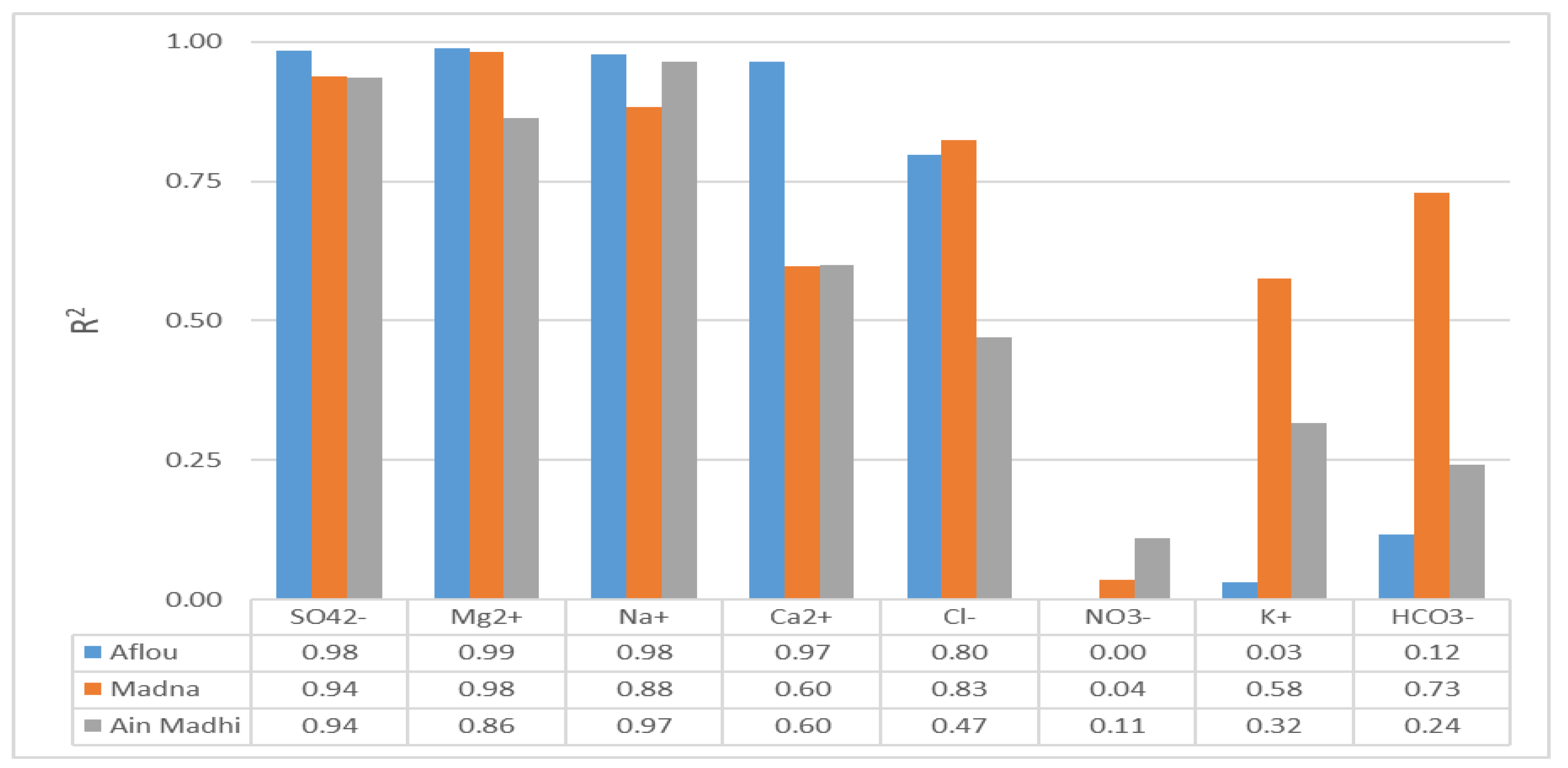

Table 1.
Features and output variables for the developed ANN models of all major ions.
| ANN Model | Features | Output |
|---|---|---|
| LMBP-MLP1 | TDS, MIN | SO42- |
| LMBP-MLP2 | TDS, MIN, SO42- | Mg2+ |
| LMBP-MLP3 | TDS, MIN, SO42- | Na+ |
| LMBP-MLP4 | TDS, MIN, SO42-, Na+, Mg2+ | Ca2+ |
| LMBP-MLP5 | TDS, MIN, SO42-, Na+ | Cl- |
| LMBP-MLP6 | TDS, MIN, SO42-, Na+ | K+ |
| LMBP-MLP7 | TDS, MIN, Mg2+ | HCO3- |
| LMBP-MLP8 | TDS, MIN, Mg2+ | NO3- |
Table 2.
Results of the developed ANN models for all major ions.
| ANN Model | Training | Validation | Test | All | ||||
|---|---|---|---|---|---|---|---|---|
| R2 | RMSE(mg/L) | R2 | RMSE(mg/L) | R2 | RMSE(mg/L) | R2 | RMSE(mg/L) | |
| LMBP-MLP1 | 0.923 | 65.730 | 0.964 | 56.970 | 0.842 | 53.660 | 0.936 | 63.368 |
| LMBP-MLP2 | 0.921 | 14.890 | 0.943 | 11.800 | 0.980 | 12.840 | 0.924 | 14.274 |
| LMBP-MLP3 | 0.916 | 20.230 | 0.927 | 17.270 | 0.759 | 14.960 | 0.916 | 19.346 |
| LMBP-MLP4 | 0.867 | 21.990 | 0.887 | 23.510 | 0.945 | 36.460 | 0.892 | 24.034 |
| LMBP-MLP5 | 0.865 | 44.640 | 0.902 | 43.600 | 0.895 | 30.530 | 0.872 | 43.296 |
| LMBP-MLP6 | 0.533 | 2.990 | 0.601 | 2.850 | 0.045 | 6.480 | 0.441 | 3.482 |
| LMBP-MLP7 | 0.300 | 64.250 | 0.630 | 37.760 | 0.366 | 41.720 | 0.330 | 59.029 |
| LMBP-MLP8 | 0.325 | 43.400 | 0.865 | 40.870 | 0.004 | 40.460 | 0.523 | 41.886 |
Table 3.
The value of charge balance (CB) and their evaluation of samples (Aflou).
| Area | SO42- Pred. |
NO3- Meas. | HCO3- Meas. |
Cl- Pred. |
Ca2+ Pred. | Mg2+ Pred. | Na+ Pred. | K+ Pred. |
CB % |
Evaluation |
|---|---|---|---|---|---|---|---|---|---|---|
| Aflou | 105 | 5 | 240 | 45 | 88 | 23 | 23 | 7 | 0.03 | Good |
| 410 | 30 | 326 | 135 | 152 | 68 | 82 | 7 | 3.54 | Good | |
| 906 | 15 | 273 | 210 | 292 | 146 | 168 | 14 | 7.45 | Moderate | |
| 393 | 14 | 239 | 190 | 153 | 61 | 86 | 7 | 3.23 | Good |
Table 4.
The value of charge balance (CB) and their evaluation of samples (Aflou).
| Area | SO42- Pred. |
NO3- Meas. | HCO3- Meas. | Cl- Meas. |
Ca2+ Pred. | Mg2+ Pred. | Na+ Pred. | K+ Meas. |
CB % |
Evaluation |
|---|---|---|---|---|---|---|---|---|---|---|
| Ain Madhi | 434 | 9 | 237 | 145 | 206 | 83 | 102 | 5 | 11.60 | Poor |
| 426 | 10 | 232 | 145 | 206 | 80 | 104 | 5 | 11.90 | Poor | |
| 123 | 13 | 212 | 70 | 95 | 27 | 28 | 2 | 0.07 | Good | |
| 124 | 16 | 185 | 93 | 95 | 27 | 28 | 2 | 1.57 | Good | |
| 1677 | 4 | 237 | 400 | 177 | 298 | 270 | 15 | 4.87 | Good | |
| 1227 | 10 | 217 | 370 | 576 | 173 | 247 | 12 | 15.28 | Poor | |
| 291 | 13 | 247 | 240 | 187 | 38 | 140 | 6 | 4.51 | Good | |
| 281 | 2 | 241 | 205 | 183 | 38 | 131 | 6 | 7.40 | Moderate | |
| 352 | 5 | 162 | 220 | 163 | 50 | 104 | 15 | 2.65 | Good | |
| 257 | 34 | 144 | 155 | 128 | 41 | 58 | 6 | 0.77 | Good |
Table 5.
The value of charge balance (CB) and their evaluation of samples (Madna).
| Area | SO42- Pred. |
NO3- Meas. |
HCO3- Pred. | Cl- Meas. |
Ca2+ Pred. | Mg2+ Pred. | Na+ Pred. | K+ Meas. |
CB % |
Evaluation |
|---|---|---|---|---|---|---|---|---|---|---|
| Madna | 888 | 7 | 230 | 354 | 199 | 142 | 221 | 12 | 1.28 | Good |
| 903 | 84 | 281 | 250 | 236 | 148 | 209 | 14 | 2.44 | Good | |
| 631 | 54 | 263 | 257 | 185 | 106 | 155 | 12 | 1.11 | Good | |
| 437 | 17 | 247 | 198 | 213 | 82 | 107 | 7 | 7.77 | Moderate | |
| 629 | 71 | 266 | 250 | 181 | 104 | 158 | 14 | 1.64 | Good | |
| 65 | 3 | 167 | 29 | 73 | 16 | 14 | 4 | 6.72 | Moderate |
Disclaimer/Publisher’s Note: The statements, opinions and data contained in all publications are solely those of the individual author(s) and contributor(s) and not of MDPI and/or the editor(s). MDPI and/or the editor(s) disclaim responsibility for any injury to people or property resulting from any ideas, methods, instructions or products referred to in the content. |
© 2025 by the authors. Licensee MDPI, Basel, Switzerland. This article is an open access article distributed under the terms and conditions of the Creative Commons Attribution (CC BY) license (http://creativecommons.org/licenses/by/4.0/).
Copyright: This open access article is published under a Creative Commons CC BY 4.0 license, which permit the free download, distribution, and reuse, provided that the author and preprint are cited in any reuse.


