Submitted:
13 March 2025
Posted:
14 March 2025
You are already at the latest version
Abstract
The market risk measurement of a trading portfolio in banks, specifically the practical implementation of the value-at-risk (VaR) and expected shortfall (ES) models, involves intensive recalls of the pricing engine. Machine learning algorithms may offer a solution to this challenge. In this study, we investigate the application of the Gaussian process (GP) regression and multi-fidelity modeling technique as approximation for the pricing engine. More precisely, multi-fidelity modeling combines models of different fidelity levels, defined as the degree of detail and precision offered by a predictive model or simulation, to achieve rapid yet precise prediction. We use the regression models to predict the prices of mono- and multi-asset equity option portfolios. In our numerical experiments, conducted with data limitation, we observe that both the standard GP model and multi-fidelity GP model outperform both the traditional approaches used in banks and the well-known neural network model in term of pricing accuracy as well as risk calculation efficiency.
Keywords:
value-at-risk
; expected shortfall
; Basel III
; FRTB
; option pricing
; multi-asset option
; Gaussian processes regression
; multi-fidelity model
; machine learning
; neural networks
MSC: 91G20, 91B05, 62G08, 60G15, 65D05
1. Introduction
Market risk refers to the risk of losses resulting from adverse movements in market prices, encompassing both on- and off-balance sheet positions. From a regulatory standpoint, market risk emanates from positions held in a bank trading book, as well as from commodity and foreign exchange risk positions within the entire balance sheet. Counterparty credit risk, on the other hand, relates to the risk that a counterparty in a transaction may get default before all the cash flows have been settled. Credit valuation adjustment (CVA) risk pertains to the risk of incurring losses due to fluctuations in CVA values triggered by changes in counterparty credit spreads and market risk factors. Financial risk management has always been a central activity in banking industry, but since the 2008 global financial crisis, it has become even more important: there is an increasing focus on how financial risks are being assessed, monitored and managed. In the last three decades, extensive research, spanning both academic and financial industry domains [13,15,16,48], has been dedicated to advancing banking practices and refining risk calculations to meet existing and forthcoming challenges.
The European Banking Authority (EBA) plays a crucial role in ensuring consistent implementation of the new regulations across the European Union, particularly with respect to the Fundamental Review of the Trading Book (FRTB) as part of the Basel III reforms [3], by developing technical standards, guidelines, and reports. Specifically, the Basel Committee on Banking Supervision introduced the FRTB framework to enhance accuracy and consistency in trading book capital requirements. This initiative has compelled banks with trading operations to swiftly implement significant changes. Banks had to reinforce their models, data management, information technology infrastructure, and processes. Additionally, capital markets businesses had to optimize product structures, adjust hedging strategies, and reprice products. For some banks, unprofitable business lines due to FRTB led to downsizing or exiting their operations. The impact of FRTB on banks is multifaceted, affecting methodologies, data management, processes, and systems. These changes pose significant challenges, particularly in areas like non-modellable risk factors and the development of default risk charge (DRC) methodologies. Simultaneously, the implementation of FRTB necessitates substantial upgrades in banking systems, including computational capacities and alignment of risk factors. The FRTB also emphasizes the importance of market and reference data quality, demanding a coherent framework for sourcing and mapping positions accurately. These interconnected challenges highlight the intricate demands faced by banks in adapting to FRTB regulatory requirements. Banks must increase computational capacities, revalue positions daily, and develop new platforms to compute standardized capital charges: significantly higher calculation capacity will be required compared to that for current value-at-risk (VaR) calculations and banks estimate an increase in number of full revaluation runs by a factor of 5 to 10 [4]. Simultaneously, the banking industry response to these complex demands involves exploring the potential of machine learning, which has gained prominence for big data management, function interpolation and exploration in various sectors. In finance, machine learning applications in, such as pricing, fraud detection, credit scoring, and portfolio management, have become increasingly significant [17,19,36]. This technological advancement offers a potential solution to the intricate challenges posed by the FRTB, offering innovative ways to adapt and streamline banking processes in the face of regulatory requirements.
A recent study by the [19] highlights the potential of machine learning in enhancing risk models by detecting complex patterns in large datasets. The neural network family, famous for its universal approximation and its customization flexibility, is applied to various financial tasks ranging from derivative pricing and hedging [10,29] to calibration [26] and partial differential equations solving [28]. [50] show improvements in the volatility forecast using neural network and GELM, where the latter is a combination of the generalized autoregressive conditional heteroskedasticity (GARCH) model and extreme machine learning (ELM) model [27], this then enhances the accuracy and efficiency in value-at-risk calculations. [46] make a survey on the application of neural network models in quantitative finance. Bayesian models such as the Gaussian process regression can be explored for the yield curve forecast and derivatives pricing [40], reducing computation time. [14] apply GP models to the fast derivatives pricing and hedging under the assumption that the market is modelled by a limited set of parameters. They provide the numerical test of European call, American put and barrier option in the variance gamma and Heston models. [23,38] replace the linear regression model in the [37] model by a Gaussian process regression to price Bermudan options. In particular, at each backward evaluation time step, they train a GP regression to estimate the time value of the option. [12] focus on the approximation of European call in the Heston model, they furthermore study the multi-output Gaussian processes (GPs) structure to simultaneously estimate various option prices underwritten on the same asset. In [34] the market value of the whole trading portfolio of different options on a common underlying is efficiently approximated by a Gaussian process regression. In a nutshell, the choice between neural networks and Gaussian process regression depends on the specific task requirements. The former is The latter is preferred when uncertainty analysis in predictions is crucial, or when there are limitations in the number of training points available. Despite these advancements, machine learning methods have not fully integrated into the financial risk measurement framework yet.
This work aligns with the research flow of [34], which produced encouraging results for the and calculation of the portfolio consisting of financial instruments written on a single asset. However, one drawback of the approach is the curse of dimensionality. As the input space dimension of the pricing function increases, the number of sampling points required to train the machine learning algorithm, used as a proxy pricing function, increases substantially. This issue becomes practically challenging when evaluating multi-asset options such as best-of, worst-of and basket options. The GP techniques applied to fixed income derivatives like Bermudan swaptions also suffer from the curse of dimensionality. At this stage, the main difficulty lies in the limitation of training data rather than the scalability of Gaussian processes model for learning large datasets (cf. Section 3.2). While the direct use of machine learning model may be efficient enough, some enhancement techniques can be applied to achieve optimal results. For example, when performing the risk calculation of an interest rate derivatives portfolio, [47] apply dimensional reduction techniques, e.g. principal component analysis (PCA) or learning from diffusive risk factors [1], to reduce the number of market risk factors before interpolating the portfolio value by Chebyshev tensors. However, when products are highly nonlinear and depend on many diffusive risk factors, e.g. multi-asset derivatives, the dimensional reduction techniques proposed in [47] may be no longer appropriate. This leads us to explore other enhancement techniques such as multi-fidelity modeling. Fidelity in modeling refers the degree of detail and precision offered by a predictive model or simulation. High-fidelity models provide highly accurate outcomes but require substantial computational resources, for instance, the pricing engine in our financial case. Due to its high cost, the use of high-fidelity models is often limited in practice. By contrast, low-fidelity models, while resulting to less accurate outcomes, are cheaply accessible and often offer some useful insights of the learning problem. By combining models of different fidelity levels, multi-fidelity modeling exploits all the information along these models and their correlation structure to provide quick yet accurate predictions. [18] do a survey of the multi-fidelity modeling. This technique can be used along with any machine learning models, such as neural networks [35,39] or Gaussian process regression [6,30,32]. In the research, we investigate multi-fidelity Gaussian process regression (mGPR). While the latter is well-known and widely used in geostatistics and physics under the name cokriging (see lecture notes in https://geostatisticslessons.com and references therein), to the best of our knowledge, we have not seen any of its application in quantitative finance. This motivates us to study this modeling for the financial application, where high-fidelity model is the derivative pricing engine and lower fidelity models can be either its simpler approximations or fast pricing engines of correlated products.
The rest of the chapter is organized as follows. Section 2 introduces the principle of market risk according to the regulation, highlighting the computational challenge in the practical implementation of VaR and ES model. Section 3 reviews the Gaussian process regression and its application in the risk calculation of the trading portfolios. Section 4 describes multi-fidelity modeling and how it works with GP model, coming along with some ideas of their application in quantitative finance. Section 5 sketches the setup and the training specification for our numerical experiments, which are reported in Section 6. Section 7 concludes our findings and provides perspectives for future research.
2. Market Risk Assessment and Computational Challenge
According to [4], market risk is defined as "the risk of losses (in on- and off-balance sheet positions) arising from movements in market prices". Market risks include default risk, interest rate risk, credit spread risk, equity risk, foreign exchange (FX) risk commodities risk, and so on. Regulatory separates market risk with other kinds of financial risk, for example, credit risks referring to the risk of loss resulting from counterparty (the party with whom the bank makes engagement in the contract) default or operational risk referring the risk of loss resulting from the failures of internal banking system. Under the FRTB framework, banks can choose either the standardized measurement method (SMM) or the internal model-based approach (IMA) to quantify their market risks. The first approach, which can be easily implemented, is not appealing to banks due to its overestimation of the capital required to cover market risks. The second approach more accurately reflects the risk sensitivities and better postulates the economic risk carried by the banking balance sheet. However, to use their own proposed internal model, banks must gain the regulatory approval through a rigorous backtesting procedure.
Under the internal model approach the calculation of capital charge is based on tail risk measures, namely value-at-risk () and expected shortfall (), of the possible loss of the holding portfolio during a certain trading period. and are measured at typically high confidence levels (for ) or (for ) in a short liquidity horizon, i.e. day or 10 days. Assume that the value of a considered trading portfolio at date t is a function of risk factors , denoted by . At date , the possible loss of the portfolio (or profit and loss), denoted by , is defined by
where is the value of portfolio at date and the approximation is probably the convention used by the bank, considering time horizon h is small, e.g. one day or ten days. By the approximation in (1), can be interpreted as the potential loss of the portfolio resulted from the shock of the risk factors . The value-at-risk at a confidence level represents the minimum capital required to cover the market risk, while the expected shortfall means the average loss given the latter exceeds the . These two risk measures are defined by
Statistical methods for calculating (2) include analytical, historical and Monte Carlo approaches ([45] Section 2.2 page 61). According to the the Monte Carlo method, is the -percentile of the set of possible losses simulated for time horizon h, while is the empirical average of losses above the . Shocks of risk factors at date are generated by synthetic dynamic models calibrated from the historical market data. The market risk calculation procedure by Monte Carlo is summarized in Algorithm 1, see also [25] for a review of risk calculation by the Monte Carlo methods.
| Algorithm 1:Calculation of and by full repricing approach |
|
input: Calibrated diffusion model, pricing engine , an actual vector of risk factors , a confidence level , time step h and a large number N
output: estimated and
Compute
Simulate N scenarios of shock using calibrated diffusion model
Compute N corresponding prices
Compute N scenarios of losses
Compute and by Monte Carlo
|
Remark 1.
In the FRTB, the calculation of market risk for a trading book by the internal model-based approach needs to be implemented for various liquidity horizons associated with different risk factors. To be more specific, for a considered portfolio, banks need to classify involved risk factors into five categories of liquidity horizons: 10, 20, 40, 60 and 120 days. The FRTB requires banks to assess market risk for these liquidity horizons by taking into account shocks to risk factors at the same and longer horizons. For example, the risk calculation for 10-day horizon must consider shocks to risk factors from all five categories, while the risk calculation for 20-day horizon needs to consider shocks at 20 days and longer. This framework provides a more comprehensive and accurate assessment of market risk, but requires a complex and time-consuming calculation process.
2.1. Computational Challenge and Applications of Machine Learning
The market risk calculation appears to be doable by Algorithm 1. Nevertheless, we have not discussed yet about the computational complexity of the pricing engine. In banks, the pricing engine of a trading derivative portfolio involves various numerical algorithms depending on the nature of the portfolio. Some products or portfolios can be rapidly priced, such as using analytical formulas or accurately fast approximations. However, when financial models and/or products of the portfolio are complex as usually the case in practice, some heavily computational algorithms need to be referenced including Monte Carlo schemes, tree methods, see for example ( [11] Chapter 6 and 7). The risk calculation using any of the algorithms mentioned above is referred to as the full repricing approach (i.e. full revaluation approach). The latter is the most accurate but very costly (for a portfolio of complex products) as the measurement of the tail risk, i.e. VaR and ES, of the portfolio needs to recall intensively the pricing engine.
In the context of implementing the and calculation using Monte Carlo simulation, banking institutions tend to avoid direct use of pricers, as it is time consuming and makes them inefficient. Certain banks prefer to use proxies based on sensitivity calculation and second-order Taylor developments to compute the possible losses of derivative portfolios [8], see Section B. Although these approaches offer performance gains, their precision is often questioned. Recently, alternative approaches have emerged that aim to strike a balance between performance and precision in risk calculation, such as value-at-risk and expected shortfall. Among these methods, the works of [12], and [14] explore the application of Gaussian process regression in finance, and [46] discuss the use of neural networks in the same context. The common idea behind these studies is to use machine learning models as interpolation tools, also known as surrogate models, to estimate derivative prices. More recently, [47] use Chebyshev polynomials as interpolators, combined with principal component analysis techniques (PCA), for financial risk calculation, aligning with the same line of though. Figure 1 illustrates the risk calculation process that employs these innovative machine learning approaches, involving only a few complete revaluations of a derivative portfolio.
2.2. Equity Options
In the remainder of this chapter, the objective is to evaluate and manage the market risk associated with a trading portfolio consisting of equity derivatives. These products are written on a stock whose the price at date t is denoted by . Among these derivative products, vanilla options, barrier options, and American options on a single underlying asset can be mentioned. In the Black-Scholes model, the values of these options are simply determined by analytical formulas depending on the underlying asset price , except the American option values for which a numerical method, e.g. binomial tree, is mandatory. The portfolio may also include multi-underlying options such as basket options, best-of options and worst-off options. For this case, we denote by the prices of d underlying assets that are governed by lognormal processes:
where r is a risk-free rate, denote the asset volatilities, and are Brownian motions with a correlation matrix . In what follows, we assume the constant risk-free rate and volatilities.
Let denote the value of the European multi-asset derivative at the maturity T, also called the payoff. Subject to the above assumptions, the value of the European multi-asset option at date t is the conditional expectation under the risk neutral probability of the discounted payoff, denoted by ,
We are particularly interested in four options whose the payoff can be written as a vanilla option payoff against a strike K given in Table 1.
Given (3), the price of geometric average options are fast referenced by the Black-Scholes formula, and the price of basket options can be accurately approximated by the Black-Scholes formula thanks to the convention that the sum of lognormal variables is approximately a lognormal variable [7]. Otherwise, the price of other options in Table 1 are evaluated by Monte Carlo simulation.
3. Gaussian Process Regression for Option Pricing
Gaussian process regression is the canonical method for Bayesian modeling of spatial functions. The method is highly recommended in cases where data is sparse because of its generalization of the Gaussian distribution from finite-dimensional vector spaces to infinite-dimensional functional spaces. Due to this principle, the model is considered as non-parametric. In this section we briefly introduce the Gaussian process regression and its application to model financial derivative products. The more background of GP model can be referenced in [44] and Chapter 15 [41].
In what follows, bold lowercase letters, e.g. , stand for vector notation, whereas bold uppercase letters, e.g. , are used for matrix notation.
3.1. Gaussian Processes Regression and Prediction
Let be a probability space, consider a random vector for a positive integer d corresponding to the dimension of inputs, and a response variable . In supervised learning, the goal is to learn a target function portraying the relation between inputs and the response variable. To this end, we assume the following regression
where are i.i.d Gaussian white noise with zero mean and variance . Different from other regression models which usually assume a parameterization form of f, the Gaussian processes place directly a multivariate normal prior on the space of functions. Implicitly, for any set of input points in , the random vector is multivariate normally distributed. More precisely, given a data set of N observations , where is taken from set , is the concatenated matrix in which each row is the row-vector of one observation of inputs. Let . In the Gaussian process regression,
where is the identity matrix of size N, is a prior mean vector parameteried by a mean function , and denotes the covariance matrix characterized by a kernel function such that .
Unless some extra knowledge about the prior mean function, for simplicity one can choose . Note that the convention is related only to the prior distribution and does not imply that the posterior distribution (the prediction) has zero mean. Similarly, we can impose some knowledge of the target function on the choice of the kernel function. For example, the exponential sine squared kernel takes into account the periodic characteristic of function ([44] pp. 92). The Matern kernel and the squared exponential kernel are the most frequently used stationary kernels ([44] pp. 83-84). The Matern kernel reads
where is the gamma function and is the modified Bessel function of the second kind. The smoothness of the approximate function is controllable through a positive parameter , i.e. (7) is once differentiable when and twice differentiable when . As tends to infinity, the Matern kernel (7) becomes infinitely differentiable and converges to the squared exponential kernel. The length-scale parameter can be a d positive vector and each component will be used to standardize a corresponding component of inputs. If the variances by column of the input are equal, the vector length-scale parameter will measure the impact of input variables into the predictive conditional variance, yielding an insight about the variable importance ([44] Section 5.1 and 6.6). Other kernel functions can be found in ( [44] Section 4). When in is observed directly from the groundtruth function f, i.e. , the white noise in (5) and its variance in above equations will be removed and this refers to the interpolation with noise-free observations. In brief, Gaussian processes provide a lot of flexibility to integrate extra knowledge of the learning problem, apart from data set , into the prior model hypothesis , which is particularly useful for financial applications.
For a matrix of test points, denoted by , the joint prior distribution of the response reads
where , ; and and are respectively covariance matrix of , and of and . Once the model is learned (see Section 3.2), the predictive (posterior) distribution of * is
where the posterior mean and variance are given as follows
Remark 2.
(i)As we will discuss in Section 3.2, the repeated computation of the inverse matrix in the learning procedure is a bottleneck of the GP model. However, in the prediction phase (cf. (9)) the matrix inversion is required only one time and it is even already computed during the learning phase. In particular, the posterior mean is numerically computed using the following linear expression, for ,
(ii)The posterior mean can be also written by the following linear combination, without the loss of generality, suppose the zero mean prior,
where (11) interprets the GP prediction of unction f at a new point, say as a linear combination from a set of N observable points However, the GPs model is not a linear interpolation since the non-linear term is incorporated in yi. Moreover, in the general case where exact observations are not accessible, the model will interpolate from the noisy observations taking into account the variance of noise. Hence GP model is considered as a powerful non-linear interpolation tool
3.2. Estimation of Model Parameters
The learning procedure of Gaussian process model involves finding the best suited parameters of the mean function , the covariance kernel function k, jointly denoted by θ and the white noise variance σ. The set of GP parameters can be estimated either by maximum likelihood or maximum a posteriori, or cross-validation method (see ( [44] Section 5.4) and ([41] Section 15.2.4)). By mean of computational facility, maximum likelihood is the the most used among these and this method is chosen to be a default method for the standard Gaussian processes. The criterion that we aim to maximize is the marginal likelihood, also called by the (model) evidence reads
Notice that the first term of (12) correspond to the data-fit can be seen as the the negative squared loss with a kernel-based weight in linear regression whereas the second term relates to the penalty of the model complexity (see [44] Section 2.4 and 5.4.1).
Maximizing the evidence (or minimizing the negative evidence) is usually solved by a global optimization method, namely BFGS ([42] Chapter 6), as in Scikit-learn Python package or by any gradient-based method such as Adam [31] in Gpytorch Python package. In any case, the numerical implementation must be done by full batch and involves reversing the covariance matrix of size whose the complexity is (using Cholesky decomposition). Contrarily, the prediction step (cf. (9)) costs only . Hence, even Gaussian process model is a great interpolation tool, the classical model is not appropriate for high-dimensional problem that requires an important amount of training points N to explore the target surface. Many innovative approaches are proposed to tackle this issue and in general they are developed through the use of low-rank approximation (or possibly decomposition) of the covariance matrix [22,49] and/or the use of other learning methods such as (stochastic) variational inference [5,24,49]. We refer the reader to the documentation of Gpytorch package on Python [21] for the detail as well as numerical implementation of these approaches.
3.3. Application to Derivative Portfolio Valuation
The application of Gaussian process regression is not restricted to evaluating mono-asset derivatives as illustrated below, but also applies to multi-asset derivatives in the same manner. However, when the number of underlying assets is high, one needs to use Monte Carlo sampling instead of the grid point sampling technique used in low-dimensional problems. The regression model can directly approximate the value of the entire portfolio without any additional computational cost for learning and prediction, regardless of the portfolio size and complexity. This is hence favorable for risk calculation applications ([9] Remark 3).
When the considered portfolio consists of a possibly large number of mono-asset derivatives, one can still use efficiently GP regression by the decomposition technique provided in [34]. More precisely, the portfolio may depend on a vector of d assets (risk factors) but each of its derivatives is underwritten on single stock. The portfolio price is the conditional expectation of the total derivative payoffs given the stock asset vector , hence, a function of . By the nature of the considered portfolio, we are able to categorize by risk factor
where is the sub-portfolio corresponding to the j-th stock. We build the approximate of each by one-dimensional Gaussian process model. To this end, for , we sample N equidistant training points of , say , in a determined range , and the corresponding price . Since this is the one-dimensional interpolation case and the price functions in finance are usually well-behaved, we only need to recall the pricing engine few times for sampling training data. For example, in the mono-asset portfolio experiments [34], the GPs can reach the good results using only . Once the learning is done, the GP price of a sub-portfolio at a new point is the predictive mean of the posterior distribution
where is determined in Remark 2
(ii)
(with the adaptation of notations). The GP price of the whole portfolio is then deduced by (13). The market risk calculation is straightforward by using the GP pricing model instead of the pricing engine in the Monte Carlo method (cf. Algorithm 1).
Remark 3.(i)For a derivative which depends on several market risk factors such as asset volatility, dividend and interest rate and so on, the bank sometimes uses the Black model for the pricing engine. In this case, we can train bring it back to the two-dimensional interpolation problem, i.e. the discounted future price and the volatility, and efficiently apply GP.
(ii)In the case of basket options, one can use the current price of (cf. Table 1) as the unique learning feature, leading to one-dimension Gaussian process regression.
(ii)When the derivative depends on many risk factors, i.e. multi-asset products. The algorithm may require a large number of training data for a good approximation. In our financial application, the time to get pricing training points (sampled by costly pricing engine) is more relevant than the model learning difficulty of GPR mentioned in Section 3.2.
4. Multi-fidelity Gaussian Processes Regression
In the previous section, we describe how to apply GPR to interpolate the surface of price function using a few number of price points. However, the number of required points increases dramatically with the number of risk factors. Suppose that we have access to other kinds of information, e.g. a weak pricing engine based on a lower number of Monte Carlo simulations or using few discretization time steps in the tree model, the question arises how to take into benefit of this knowledge in modeling. For this purpose, we investigate multi-fidelity Gaussian process regression (mGPR) that allows us to learn the ground truth target from several information sources, each with a different level of fidelity. Any detail of this model can be found in [6,30,32].
Assuming that we have s data sets, denoted by , sorted by increasing level of fidelity (i.e. is the most accurate and expensive data whereas is the most simplified and abundant data). In [30], the autoregressive model is used to model the cross-correlation structure between different levels:
where are scalar correlation parameters between and , measures the mismatch between j and and ϵ is the while noise of the lowest fidelity model. In mGPR, is supposed independent of . The goal of the model is to lean which is the relationship between the input and the highest fidelity response.
4.1. Two-fidelity Gaussian Process Regression Model
In this section, we focus on the mGPR with two fidelity levels. Let assume a data set of low-fidelity points, denoted by and a second set of high-fidelity points, denoted by , such that last points of low-fidelity data coincides with high-fidelity data, i.e.
The multi-fidelity modeling involves the following regression functions
where the parameter ρ describes the correlation of the high- and low-fidelity data, is a Gaussian process model of against and δ is the second GP model conditionally independent with the former. In what follows, we consider GP models with constant prior mean [20,30] parameterized by coefficient β, Marten kernel covariance function with and parameterized by θ as per (7), and a multiplicative form of the marginal variance . In particular, the prior model is
and
where l and ξ are mean vectors and , and the covariance matrices . Hence the multi-fidelity model is characterized by the parameters of the first and second Gaussian processes: and , and the correlation parameter ρ.
4.2. Illustrative Application of Multi-Fidelity Model in Option Pricing
For the pricing and risk calculation problem, our proposed approach is to learn the pricing engine, cf. the high fidelity model, with the less precise price values, cf. lower fidelity data. For instance, if the pricing engine involves Monte Carlo simulation of paths, we can sample weak price values calculated by only, e.g. 100 paths as low-fidelity data (see Section 6.2 for numerical experiments). In the American option pricing case, where the accurate price value is calculated using a binomial tree with 100 time steps, the weaker price can be generated by a sparser tree with only, e.g. 10 time steps. Conversely, if the target is the American option, which is expensively computed by tree model, its European counterpart, which is quickly evaluated using the Black-Scholes formula, can serve as lower fidelity data.
Remark 4.[2] propose an analytic approximation of an American option which is equal to the value of its European counterpart plus an add-on or their intrinsic values with a switch condition detailed in Section A.
Figure 2 and Table 2 demonstrate the numerical test of an American put of strike 62. The configuration of this experiment is detailed in Section 5 and Section 6.1. In particular, the GPR is trained with only 5 American put prices, while the mGPR integrates additionally 10 European prices as low-fidelity data. All training points are drawn from a regular grid of the underlying asset within an interval, and test points are uniformly sampled within the same interval. We observe a significant mismatch of the GPR estimate (cf. blue curve), notably in the in-the-money region, whereas the mGPR estimate (cf. yellow curve) satisfactorily fits the American put price computed using a binomial tree with 100 time steps. Additionally, the mGPR provides smaller prediction uncertainty represented by the light yellow interval, which closely aligns with the yellow curve and is visually indistinguishable in Figure 2. For further comparison, we also implement a second standard GPR, learning the discrepancy between American and European prices, and the approximation introduced in [2] (see Section A). Their results are then reported in Table 2.
4.3. Conditional Distribution of the Estimate
We describe now the posterior mean and variance of the prediction once the model is completely learned. Following the demonstration in Appendix A [20], for a new point , the prediction of the high-fidelity model follows normal distribution:
with mean and variance functions:
where
In addition, is the covariance function between and
and the covariance matrix of vector reads
We can notice that the computation of (21) involves reversing the massive covariance matrix of size . To reduce the computational complexity, one can apply the Schur complement of block matrix which is thus presented by Proposition 3.1 in [32].
Instead of performing the inversion matrix in (24) which has a complexity of , the computation of in (25), involving the inverse of and , has a much lower complexity of . By substituting (25) into (21) and doing some calculus, one can simplify the above formulas as follows
yielding the posterior mean and variance
4.4. Bayesian Estimation of Model Parameters
Due to the conditional independence assumption in the second line of (17), the first set can be separately learnt by, for example, the maximum likelihood method using data set . While the parameters of the second Gaussian processes and the correlation parameter ρ need to be jointly estimated to carry out the idea of formulation (17) ([32] Section 3.3.2). Similarly to (12), the parameters of the low-fidelity model are estimated by maximizing the following log-likelihood
Differentiating the above equation w.r.t. and and solving it at 0 yield
and
To learn the second Gaussian process model, we define
The log-likelihood of the model reads
yieling the MLEs of
To compute the above parameters, one needs to estimate by solving the following optimization
Note that (36) can be directly solved by numerical methods mentioned in Section 3.2 since the inversion of the small matrix of size is not problematic. While the same procedure may not be applied for system (31) when the number of low-fidelity is large. We then present in the next subsection the sparse Gaussian process model for low-fidelity model.
5. Experiment Design and Model Specification
In this section, we present numerical tests dedicated to evaluating the accuracy and performance of the algorithms studied earlier in this chapter. More specifically, these experiments are conducted on two trading portfolios (cf. Section 6.1 and Section 6.3), interspersed by an examination of individual multi-asset calls (cf. Section 6.2). The first one concerns a portfolio of single underlying derivatives, including plain vanilla (call and put), barrier and American options. The second one consists of multi-asset options, such as geometric, basket, best-of- and worst-of- options. The comparison is based on benchmark methods and scores explained below. We conclude this section by specifying the model of the implemented algorithms.
First, we analyze the case of the single-asset options portfolio described in [34]. This portfolio, with a time maturity of ten years, consists of 100 distinct calls and puts issued on each of the four considered underlying assets. In particular, each asset is used to write 10 vanilla, 10 barrier and 5 American options with their strikes randomly generated from 60 to 140. More details about market and product parameters in the portfolio are presented in Tables 1 and A.1 [34]. We then evaluate the price of each multi-asset option, as indicated in Table 1. Each option expires after two years and is based on the same five assets. The actual values of geometric call options can be calculated using the Black-Scholes formula and serve as a reference. In the case of high dimensionality, the considered portfolio comprises 500 derivatives, depending on the performance of 20 stocks, generating a total of 20 market risk factors. Each derivative is characterized by various parameters, including a random selection of underlying assets from 2 to 20, a strike price ranging from 80 to 160, and a number of options from 100 to 500. It is noteworthy that each derivative can be either a call or a put option among the four types introduced in Section 2.2. The portfolio maturity is set at 5 years, meaning that all its derivatives have a maturity ranging from 6 months to 5 years. In the Black-Scholes model framework, we choose a risk-free rate of . Initial asset prices are arbitrarily chosen within a range of 100 to 120, and the volatility of these assets is set to vary between 0.2 and 0.5 with a random correlation matrix, refer to Table 3 and Figure 3. Finally, we examine the pricing and risk calculation problem for different time horizons, namely one day, ten days, and one month. At longer horizons, the magnitude of shocks and their volatilities increase, leading to a significant challenge in adapting the number of interpolation points. Financially, the price function becomes less linear, and the tail of the potential loss distribution becomes heavier.
5.1. Benchmarking
For the numerical implementation of market risk metrics calculation, the full pricing approach uses paths in any case. This level is chosen to ensure a satisfactory level of convergence of high quantiles estimation. However, a limited number () of these prices is chosen to train the machine learning models.
Regarding the exact pricing engine, the value of vanilla and barrier options in the mono-asset derivatives portfolio are calculated by analytical formulas, while the binomial tree with 100 time steps is used to evaluate American options. For multi-asset options, the exact pricing engine is defined by a Monte Carlo simulation of paths, except for geometric options whose the price can be computed by the Black-Scholes formula.
We implement the sensitivity-based pricing approximation (SxS) in Section B. To get sensitivities data, we shock relatively of each risk factor and use the central finite difference, yielding totally 40 portfolio evaluations for the first order sensitivity-based approach. The second order sensitivities are numerical unstable and lead to a worse approximation of the price. Hence they are not considered in our numerics.
Regarding machine learning methods, we implement a two-hidden-layer neural network (see Section C) (NN) and two Gaussian process models introduced in Section 3 (GPR) and Section 4 (mGPR). In the latter, the high-fidelity data consists of the Monte Carlo paths prices, while the low-fidelity comprises weak prices based on 100 MC paths in Section 6.2 and 500 MC paths in Section 6.3. For measuring the pricing mismatch, we use the mean absolute percentage error (MAPE) over scenarios in the and computation:
where and are respectively actual price (i.e. analytical or Monte Carlo price) and predicted price (e.g. GPR approximative price), and is the actual price without shock. The MAPE evaluating the average relative error of the estimate and the true observation is a common choice for benchmarking in finance. For risk assessment purpose, we measure the error of value-at-risk and expected shortfall calculated based on surrogate models (i.e. and ) against the full revaluation ones calculated based on actual prices (i.e. and ). For the relative measure, the error is then standardised by today price
Finally, the computation time is also reported to compare the resource efficiency.
5.2. Model Specification
For neural network model, we train a two-hidden-layer Relu network of 50 hidden units (cf. Section C). We observe numerically that more complex architectures do not significantly improve the approximation performance. Network parameters are calibrated by the stochastic gradient descent algorithm, i.e. Adam optimizer [31], using 2000 epochs. The learning rate is set at and each batch takes one fifth of the training data size.
The standard Gaussian process regression is trained using the scikit-learn Python package. We set a zero mean prior distribution and use Matern kernels with (see (7)) to model the covariance matrix. A single length-scale is selected; however, the input is normalized by subtracting its empirical mean and then dividing by its empirical standard error. The optimization is restarted 5 times for the numerical stability. To implement multi-fidelity Gaussian process regression, we use emukit package [43] which is built upon the Gpy framework developed by machine learning researchers from the University of Sheffield. The model configuration is either set as the standard Gaussian processes or left at its default. The optimization is rerun 5 times.
6. Numerical Results
The main aim of this section is to provide a numerical analysis of algorithms based on Gaussian process regression (GPR) and the multi-fidelity model (mGPR) when applied to the repeated valuation and market risk calculation of an equity trading portfolio. It is worth emphasizing that a key advantage of the proposed new methods is that valuation and risk assessment are performed at the portfolio level, rather than on a deal-by-deal basis, which is the case with traditional approaches.
6.1. Mono-Asset Options Portfolio Case
Figure 4 and Figure 5 and Table 4 outline the performance of Gaussian Process Regression (GPR) in the full revaluation and risk calculation of a mono-asset portfolio with the sub-portfolio techniques outlined in Section 3.3. The accuracy of the GPR is evident in both pricing and risk calculation. For this mono-asset experiment, we train the regression models by a regular grid and backtest with more (uniformly) random data [14,34]. In particular, the training and test stock prices are shocked around their initial values using their diffusion models, e.g.
where and h denote respectively the initial stock price and volatility of the i-th asset, and the common interest rate and time step.
In Figure 4 and Figure 5, a precise fit of the price function is achieved when employing 5 points or more for training each sub-portfolio. The risk measures estimated by the GPR approach consistently converge to the benchmark measures obtained by the full revaluation approach, i.e. the intensive Monte Carlo method with 100,000 paths. The latter takes approximately 2 hours and 25 minutes on our machine. When learning from 10 points (resp. 5 points), the GPR achives a speed up of 1,000 times (resp. 2,000 points) compared to the full revaluation approach. The high runtime of the full revaluation approach in this experiment is primarily due to the American pricing calculations using a binomial tree with 100 time steps. This section concludes the performance of the Gaussian process regression in the mono-asset portfolio pricing and risk calculation.
6.2. Multi-Asset Options Case
Figure 6 and Table 5 display the results of the pricing and risk calculation for a five-asset geometric average call. Both GPR and mGPR models are trained using Monte Carlo prices with 100,000 paths, while the analytical prices are used as a reference for backtesting. Additionally, mGPR uses 200 prices obtained through the Monte Carlo method with 100 paths as low-fidelity data, which is still less expensive than one price point used 100,000 paths. The top left plot in Figure 6 shows that two GPR models trained with 50 points can outperform Monte Carlo prices. The error decreases, reaching 10 basis points at 200 training points. Notably, mGPR outperforms GPR at lower numbers of data points before their error curves converge.
The quantile-quantile (q-q) plots in Figure 6 trace the left tail of the simulated price distribution below the 10th percentile, corresponding to the right tail of the loss in the risk calculation in Table 5. Despite the Monte Carlo price having a higher MAPE error compared to GPR prices, its tail perfectly matches the true price. The tails of GPR and mGPR prices also converge as the number of training points increases. We stop the convergence curve of mGPR at 200 training points (corresponding to high-fidelity data) because we only use 200 low-fidelity points. In Table 5, the one-day and estimated by GPRs using 200 data points have an error of around 7 basis points. Notably, GPR models significantly save time in risk calculation, including sampling and training time with 200 points (13 seconds for GPR compared to 7488 seconds for the brute force Monte Carlo approach). The mGPR model remains an effective approximation for risk measurement, especially in cases of high pricing engine costs, such as with complex portfolios, and when using minimal price points is preferred.
Figure 7, Figure 8 and Figure 9 and Table 6, Table 7 and Table 8 show the results for other options, with similar computational times to those in Table 5. Most of the remarks made in the geometric average call case are still valid for these other cases. In the arithmetic average basket call case, the risk measures computed by two GPR models have an error of about 23 basis points, which is less than 10 basis points in the two other cases. These above errors can be computed by applying results in Table 6, Table 7 and Table 8 into (37).
6.3. Multi-Asset Options Portfolio Case
Figure 10 and Table 9 illustrate the results of a multi-asset options portfolio . The time horizon of the value-at-risk and expected shortfall is set at one day. The second-order sensitivity-based approach (SxS) and the neural network learning from 40 points are not reported here due to their low precision. The learning of mGPR incorporates 500 prices computed by 500 Monte Carlo paths as low-fidelity data. Despite the portfolio complexity, both GPR models (GPR and mGPR) achieve impressive results with only 40 points. The GPR model has a MAPE of , slightly outperformed by the mGPR model with a MAPE of . While SxS performs about 10 times worse with an error of . Figure 10 highlights this difference, showing that the predicted left tail of SxS prices diverges significantly from the true price represented by the red diagonal line. While the predicted left tails of GPR and mGPR prices are not perfect, but they still concentrate around the tail of the true price, i.e. the red line.
In Table 9, mGPR predictions offer more accurate estimates of the and compared to GPR predictions, with errors of 34bps and 32bps, respectively, versus 54bps for both errors in GPR. As more data becomes available, the performance of all models improves. Generally, two GPR models outperform NN, with a MAPE of () compared to the one of NN’s () when learning with (). The difference is more pronounced in the prediction of the left tail, as seen in the two bottom plots in Figure 10. The left tails predicted by GPR and mGPR closely align with the true one, while NN underestimates the left tail. When trained with , mGPR’s errors in risk measures, around 30bps, are only half of GPR’s errors. However, this difference disappears when training with .
Table 10 displays the runtime for various risk calculation methods on our server with an Intel(R) Xeon(R) Gold 5217 central processing unit (CPU) and a Nvidia Tesla V100 graphics processing unit (GPU). The full repricing approach involves simulating scenarios of shock, with each scenario being a Monte Carlo simulation of paths computed over 500 derivatives. Without advanced programming on the GPU, the sampling procedure in banks may take up to one day. Alternative approaches show significant computational performance gains. For instance, standard Gaussian processes regression achieves a speedup of 230 times compared to the full repricing approach when learning with points, i.e. a total of 2.6 comparing to 600 seconds. Despite mGPR’s longer learning times (i.e. 56 when learning with ), its computational efficiency compared to full repricing remains remarkable. It is important to note that, under realistic constraints of the more time-consuming pricing engine in banks, the mGPR approach may take a bit longer than the GPR approach for the learning procedure, but it provides better precision in risk calculation, especially when limiting the use of the pricing engine. Table 11 and Table 12 and Figure 11 and Figure 12 correspond to the risk assessment results for a ten-day and one-month horizon, and observations from the one-day horizon case hold true for other time horizons.
7. Conclusions
We have introduced statistical and machine learning tools to handle the repeated valuation of extensive portfolios comprising linear and non-linear derivatives. To be more precise, we applied a Bayesian non-parametric technique, known as Gaussian process regression (GPR). To evaluate the accuracy and performance of these algorithms, we have considered a multi-asset options portfolio and a portfolio of non-linear derivatives, including vanilla and barrier/American options on an equity asset. The numerical tests demonstrated that the GPR algorithm outperforms pricing models in efficiently conducting repeated valuations of large portfolios. It is noteworthy that the GPR algorithm eliminates the need to separately revalue each derivative security within the portfolio, leading to a significant speed-up in calculating value-at-risk (VaR) and expected shortfall (ES). This independence from the size and composition of the trading portfolio is remarkable. Consequently, we argue that it is more advantageous for banks to construct their risk models using the power of GPR techniques in terms of calculation accuracy and speed-up.
Moreover, we have investigated multi-fidelity modeling technique and have explored its applications in pricing and risk calculation, a relatively novel concept in quantitative finance. The multi-fidelity modeling approach leverages limited access to the price engine while incorporating information from other related, more affordable resources to enhance the approximation. Trained regression models offer price estimates at the portfolio level, making them more favorable for risk calculation compared to classical pricing approaches that evaluate products individually. Our numerical findings indicate that machine learning models such as neural networks and Gaussian process regression provide more accurate results and significant time savings compared to traditional sensitivity-based approaches, maintaining precision in risk calculation akin to the full repricing approach. With the limitation of training price data, GPR models yield more impressive results than neural network. Despite the longer learning time required for mGPR, especially when low-fidelity data is available, it yields better or at least equal precision compared to the standard GPR model. Notably, as multi-fidelity modeling is not yet well-known in quantitative finance, it presents an intriguing direction for research, allowing scientists to explore traditional relationships in finance to define low-fidelity models and enhance the learning process.
Future research delves into other topics and applications of algorithms such that Gaussian process regression and multi-fidelity modeling, with a particular focus on the fixed income portfolio. We also envisage the use of the replicating portfolio value, assumed to be accessible, as low-fidelity data to leverage the learning of the target portfolio value. Additionally, the price of European basket options can serve as low-fidelity data to approximate the price of their American/Bermudian counterparts. The Black-Scholes price of derivatives can be used to improve the approximation of their Heston price. We leave these interesting applications there for future study.
Appendix A Barone-Adesi and Whaley Approximation of American Option Values
In contrast to European options, American ones grant the holder the right to exercise the contract at any time up to the expiration date. This leads to a more complicated mathematical problem when pricing American options, for which we need to use some numerical methods, such as tree models with high time steps as mentioned in Section 2.2 and Section 6.1. For this reason, pioneers in quantitative finance have looked for a way to approximate the American option values. Among them, [2] propose an analytical approximation of American option value based on the price its European counterparts, as presented below.
For a European call (put) of strike K, maturity T and underlying asset following log normal dynamic (cf. (3)), its value () is computed by the well-known Black-Scholes formula:
where
with r is risk-free rate, σ is the asset volatility and Φ is cumulative density function of the standard normal variable.
where
with and satisfy
Appendix B Sensitivity-Based Pricing Approximation
In order to measure the market risk by Monte Carlo without recalling expensive pricing engine, many banks use Taylor approximation for portfolio evaluation. This technique is also known as delta-gamma approximation method in literature [8,9]. With the same notation used in Section 2, for each scenario of underlying assets , the corresponding value of the portfolio is approximated by
where Δ and Γ are, respectively, the gradient (i.e. delta) and Hessian matrix (i.e. gamma) of the portfolio value with respect to risk factor , and . Because of the nature of (A7), pioneers in banks usually call this pricing approximation by sensitivities times shocks, abbreviated by SxS. In practice, Δ and Γ are not analytically available in closed form and they are usually estimated by finite difference (or bump and revalue) in practice. If there are d risk factors affecting the portfolio, then one needs to recall the price engine times for estimating Δ by central finite difference [Chapter 8 [11] and additionally times for estimating Γ. This approximation pricing approach provides a significant computational improvement in risk calculation for small and medium numbers of risk factors d, i.e. less than 100. However, its precision can reach an acceptable level once several conditions are met: the portfolio value is well-approximated by a linear or quadratic functions of risk factors; the shocked risk factors remain locally in the neighborhood of their initial values ; and the Δ and Γ must be accurately estimated.
Appendix C Neural Network Regression
Alongside Gaussian processes, the neural network is also a powerful non-linear model for interpolation. Different to GP regression, the neural network can be learned quickly and is scalable with the number of training points, however the model requires a sufficient training data set to learn. In this section, we provide the main notation and concept of neural networks referring the reader to [33] for a detailed presentation.
We denote by neural network family of h hidden layers, u hidden units and activation function σ, furthermore, this family maps input vectors in to output vectors in . Functions in this family are represented by the following sequential mapping (see also Figure A1),
This family of functions is parameterized by weights and biases . We denote the set of trainable parameters as . Additionally, nonlinear activation function σ, element-wisely applied, plays a crucial role in establishing the complex mapping between inputs and outputs of the network. The rectified linear unit function (Relu), i.e. is usually chosen, that is also our case, because of its generalisation property Section 6.3.1 [33].
Given a set of training data , the neural network regression looks for minimizing the following mean square error
References
- Abbas-Turki, L., S. Crépey, and B. Saadeddine (2023). Pathwise CVA regressions with oversimulated defaults.Mathematical Finance 33(2), 274–307.
- Barone-Adesi, G. and R. E. Whaley (1987). Efficient analytic approximation of american option values. the Journal of Finance 42(2), 301–320.
- Basel Committee on Banking Supervision (2013). Fundamental review of the trading book: A revised market risk framework. Available at https://www.bis.org/publ/bcbs265.pdf.
- Basel Committee on Banking Supervision (2019). Minimum capital requirements for market risk. Available at https://www.bis.org/bcbs/publ/d457.pdf.
- Blei, D. M., A. Kucukelbir, and J. D. McAuliffe (2017). Variational inference: A review for statisticians.Journal of the American statistical Association 112(518), 859–877.
- Brevault, L., M. Balesdent, and A. Hebbal (2020). Overview of gaussian process based multi-fidelity techniques with variable relationship between fidelities, application to aerospace systems.Aerospace Science and Technology 107, 106339.
- Brigo, D., F. Mercurio, F. Rapisarda, and R. Scotti (2003). Approximated moment-matching dynamics for basket-options pricing.Quantitative Finance 4(1), 1–16.
- Britten-Jones, M. and S. M. Schaefer (1999). Non-linear value-at-risk.Review of Finance 2(2), 161–187.
- Broadie, M., Y. Du, and C. C. Moallemi (2015). Risk estimation via regression.Operations Research 63(5), 1077–1097.
- Buehler, H., L. Gonon, J. Teichmann, and B. Wood (2019). Deep hedging. Quantitative Finance 19(8), 1271–1291.
- Crépey, S. (2013). Financial Modeling, A Backward Stochastic Differential Equations Perspective. Springer Finance Textbook Series.
- Crépey, S. and M. Dixon (2019). Gaussian process regression for derivative portfolio modeling and application to CVA computations.Journal of Computational Finance 24(1), 1–35.
- Culkin, R. and S. R. Das (2017). Machine learning in finance: the case of deep learning for option pricing. Journal of Investment Management 15(4), 92–100.
- De Spiegeleer, J., D. B. Madan, S. Reyners, and W. Schoutens (2018). Machine learning for quantitative finance: Fast derivative pricing, hedging and fitting. Quantitative Finance 18(10), 1635–1643.
- Dowd, K. (2003). An introduction to market risk measurement. John Wiley & Sons.
- Dowd, K. (2007). Measuring market risk. John Wiley & Sons.
- Ferguson, R. and A. Green (2018). Deeply learning derivatives. CompSciRN: Artificial Intelligence (Topic). .
- Fernández-Godino, M. G., C. Park, N.-H. Kim, and R. T. Haftka (2016). Review of multi-fidelity models. . arXiv:1609.07196.
- Financial Stability Board (2017). Artificial intelligence and machine learning in financial services: Market developments and financial stability implications. Available at https://www.fsb.org/wp-content/uploads/P011117.pdf. .
- Forrester, A. I. J., A. Sóbester, and A. J. Keane (2007). Multi-fidelity optimization via surrogate modelling. the Royal Society A: Mathematical, Physical and Engineering Sciences 463, 3251 – 3269.
- Gardner, J., G. Pleiss, K. Q. Weinberger, D. Bindel, and A. G. Wilson (2018). Gpytorch: Blackbox matrix-matrix Gaussian process inference with GPU acceleration. Advances in neural information processing systems 31, 7576–7586.
- Gardner, J., G. Pleiss, R. Wu, K. Weinberger, and A. Wilson (2018). Product kernel interpolation for scalable Gaussian processes.International Conference on Artificial Intelligence and Statistics 84, 1407–1416.
- Goudenège, L., A. Molent, and A. Zanette (2021). Variance reduction applied to machine learning for pricing Bermudan/American options in high dimension. Oleg Kudryavtsev, Antonino Zanette. Applications of Lévy Processes. .
- Hoffman, M. D., D. M. Blei, C. Wang, and J. Paisley (2013). Stochastic variational inference.Journal of Machine Learning Research 14, 1303–1347.
- Hong, L. J., Z. Hu, and G. Liu (2014). Monte carlo methods for value-at-risk and conditional value-at-risk: a review. ACM Transactions on Modeling and Computer Simulation (TOMACS) 24(4), 1–37.
- Horvath, B., A. Muguruza, and M. Tomas (2021). Deep learning volatility: a deep neural network perspective on pricing and calibration in (rough) volatility models. Quantitative Finance 21(1), 11–27.
- Huang, G.-B., Q. -Y. Zhu, and C.-K. Siew (2006). Extreme learning machine: theory and applications. Neurocomputing 70(1-3), 489–501.
- Huré, C., H. Pham, and X. Warin (2020). Deep backward schemes for high-dimensional nonlinear PDEs. Mathematics of Computation 89(324), 1547–1579.
- Hutchinson, J. M., A. W. Lo, and T. Poggio (1994). A nonparametric approach to pricing and hedging derivative securities via learning networks.The journal of Finance 49(3), 851–889.
- Kennedy, M. C. and A. O’Hagan (2000). Predicting the output from a complex computer code when fast approximations are available. Biometrika 87(1), 1–13.
- Kingma, D. P. and J. Ba (2015). Adam: A method for stochastic optimization. The 3rd International Conference on Learning Representations. .
- Le Gratiet, L. (2013). Multi-fidelity Gaussian process regression for computer experiments. Ph. D. thesis, Université Paris-Diderot-Paris VII.
- LeCun, Y., Y. Bengio, and G. Hinton (2015). Deep learning.Nature 521(7553), 436–444.
- Lehdili, N. Oswald, and H. Gueneau (2019). Market risk assessment of a trading book using statistical and machine learning. . [CrossRef]
- Li, S., W. Xing, R. Kirby, and S. Zhe (2020). Multi-fidelity bayesian optimization via deep neural networks. In H. Larochelle, M. Ranzato, R. Hadsell, M. Balcan, and H. Lin (Eds.), Advances in Neural Information Processing Systems, Volume 33, pp. 8521–8531. Curran Associates, Inc.
- Liu, S., C. W. Oosterlee, and S. M. Bohte (2019). Pricing options and computing implied volatilities using neural networks.Risks 7(1), 16.
- Longstaff, F. A. and E. S. Schwartz (2001). Valuing American options by simulation: a simple least-squares approach. The review of financial studies 14(1), 113–147.
- Ludkovski, M. (2018). Kriging metamodels and experimental design for Bermudan option pricing. Journal of Computational Finance 22(1), 37–77.
- Meng, X. and G. E. Karniadakis (2020). A composite neural network that learns from multi-fidelity data: Application to function approximation and inverse pde problems. Journal of Computational Physics 401, 109020.
- Mu, G., T. Godina, A. Maffia, and Y. C. Sun (2018). Supervised machine learning with control variates for american option pricing.Foundations of Computing and Decision Sciences 43(3), 207–217.
- Murphy, K. P. (2012). Machine learning: A probabilistic perspective. The MIT Press.
- Nocedal, J. and S. J. Wright (1999). Numerical optimization. Springer.
- Paleyes, A., M. Mahsereci, and N. D. Lawrence (2023). Emukit: A python toolkit for decision making under uncertainty. Proceedings of Python in Science Conference 22, 68–75.
- Rasmussen, C. E. and C. K. Williams (2006). Gaussian Processes for Machine learning. The MIT Press.
- Roncalli, T. (2020). Handbook of Financial Risk Management. Chapman and Hall/CRC.
- Ruf, J. and W. Wang (2019). Neural networks for option pricing and hedging: A literature review. Journal of Computational Finance 24(1), 1–46.
- Ruiz, I. and M. Zeron (2021). Machine Learning for Risk Calculations: A Practitioner’s View. John Wiley & Sons.
- Saunders, A., M. M. Cornett, and O. Erhemjamts (2021). Financial institutions management: A risk management approach. McGraw-Hill.
- Titsias, M. (2009). Variational learning of inducing variables in sparse Gaussian processes. Proceedings of Machine Learning Research 5, 567–574.
- Zhang, H.-G., C. -W. Su, Y. Song, S. Qiu, R. Xiao, and F. Su (2017). Calculating value-at-risk for high-dimensional time series using a nonlinear random mapping model. Economic Modelling 67, 355–367.
Figure 1.
Risk calculation procedure.
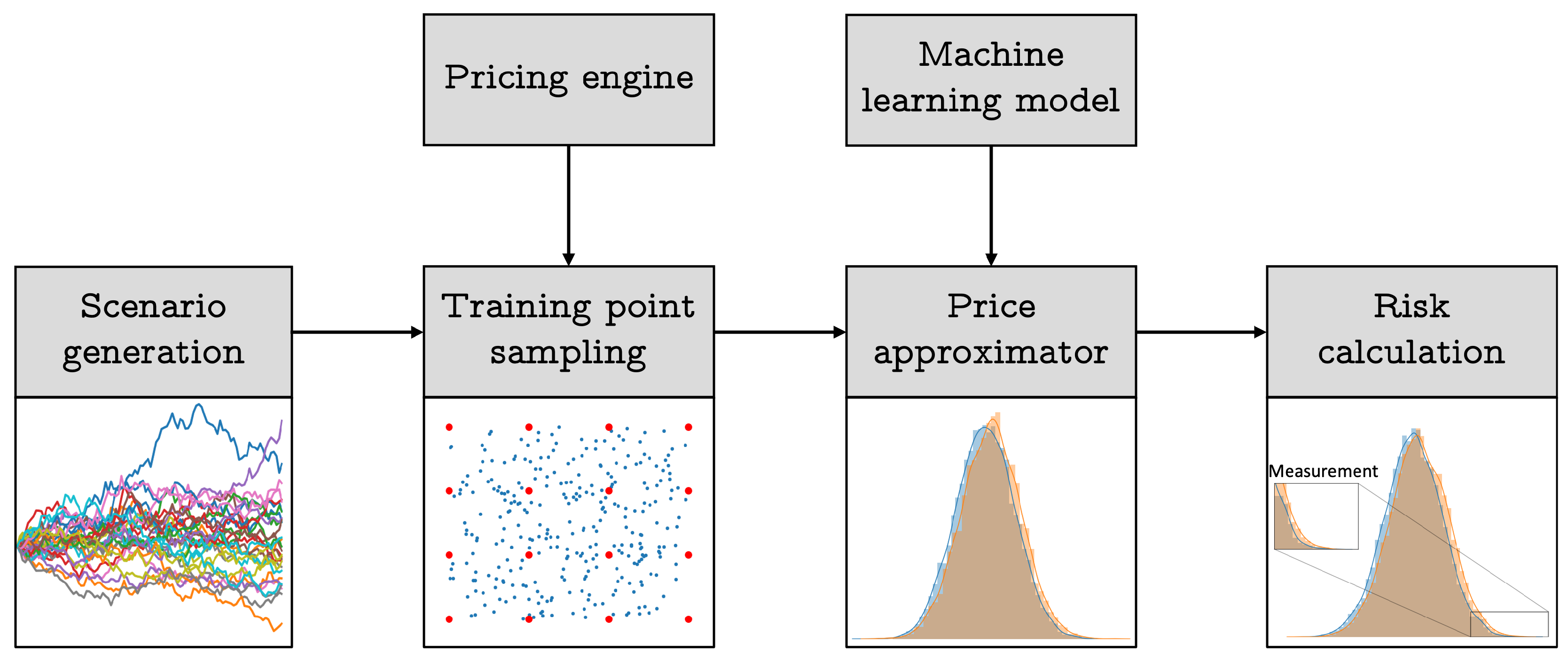
Figure 2.
American put prices predicted by GPRs learned from 5 points. Red circles represent training points in GPR and high-fidelity points in mGPR, and green inverted triangles are low-fidelity points in mGPR. The light blue and light yellow (very close to yellow curve) regions depict the uncertainty of the GPR and mGPR predictions respectively.
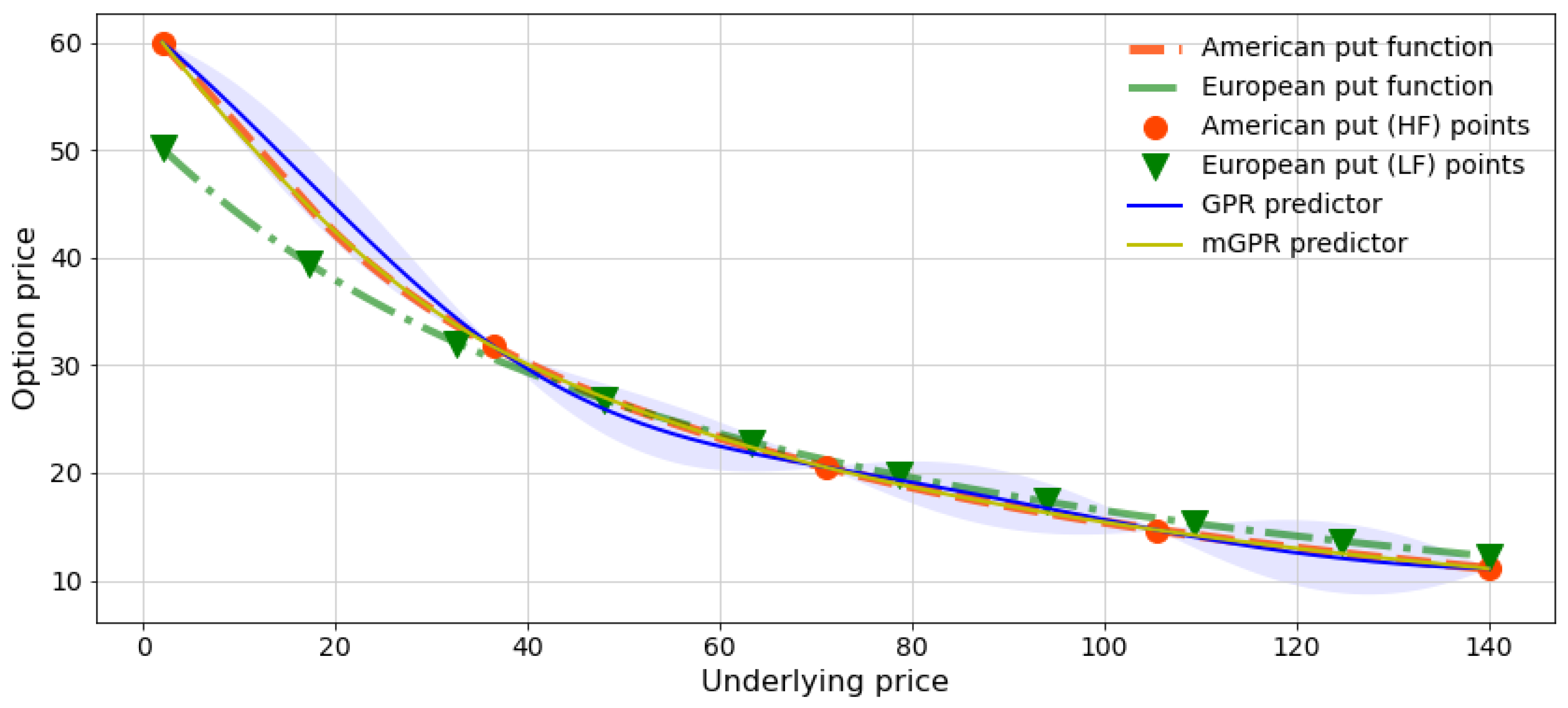
Figure 3.
Heatmap of the stock covariance matrix.
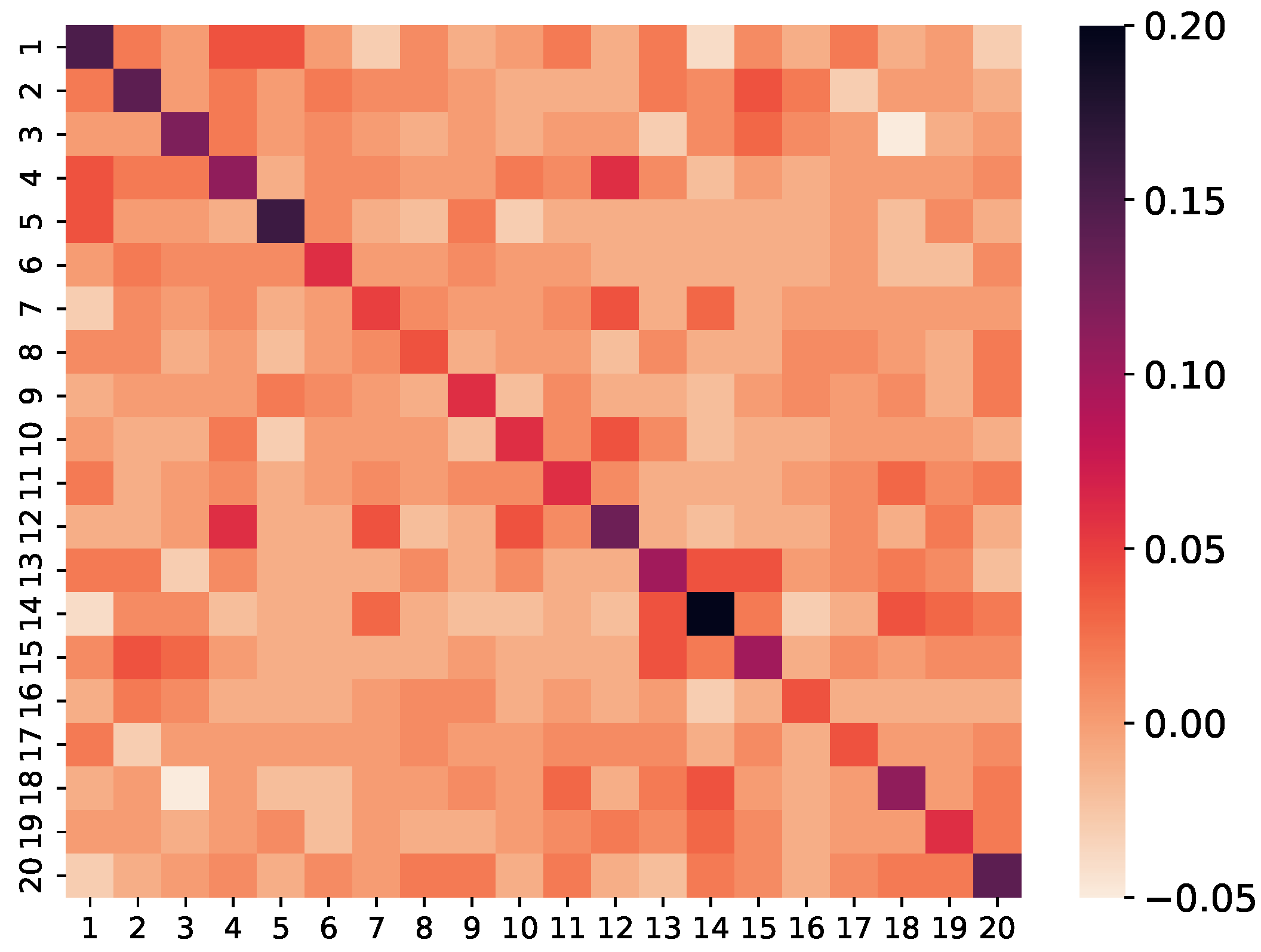
Figure 4.
Convergence of MAPE of GPR estimates when increasing the number of training points in mono-asset portfolio case.
Figure 4.
Convergence of MAPE of GPR estimates when increasing the number of training points in mono-asset portfolio case.
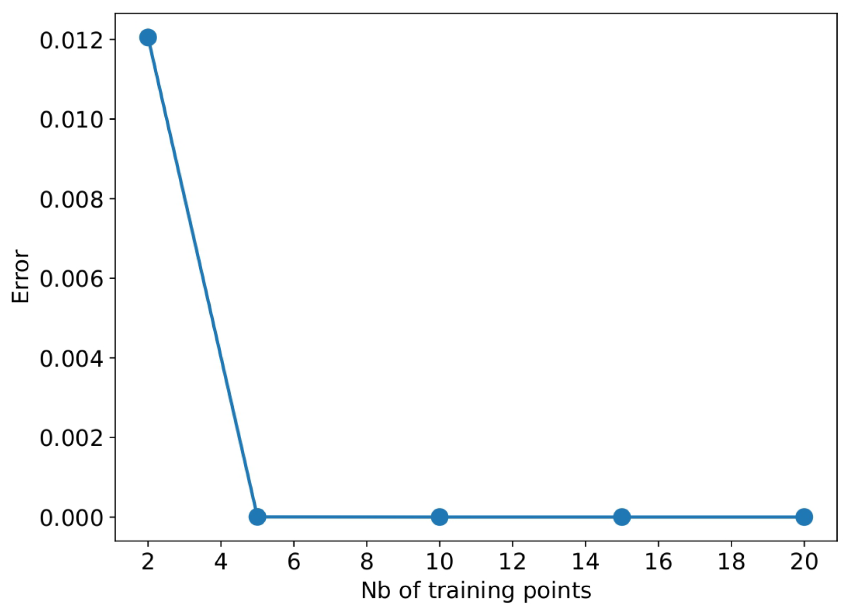
Figure 5.
q-q plots of GPR predicted price using 5 (Left), 10 (Center) and 20 (Right) training points against the true price, i.e. analytical and binomial tree prices, in the mono-asset portfolio case.
Figure 5.
q-q plots of GPR predicted price using 5 (Left), 10 (Center) and 20 (Right) training points against the true price, i.e. analytical and binomial tree prices, in the mono-asset portfolio case.
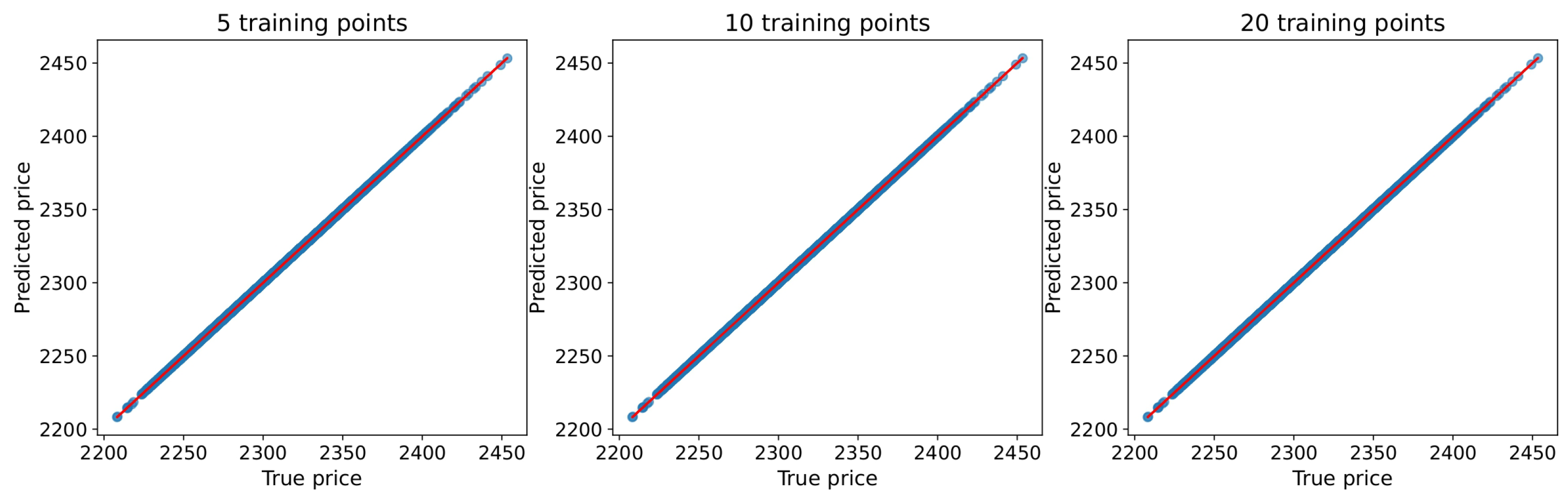
Figure 6.
MAPE of estimates of 5-asset geometric average call as a function of the number of training points (Top Left) and q-q plots comparing predictors learned from 50 (Top Right), 100 (Bottom Left) and 200 (Bottom Right) points against the true price, i.e. Black-Scholes price, below their quantile levels. The mGPR uses 200 low-fidelity points.
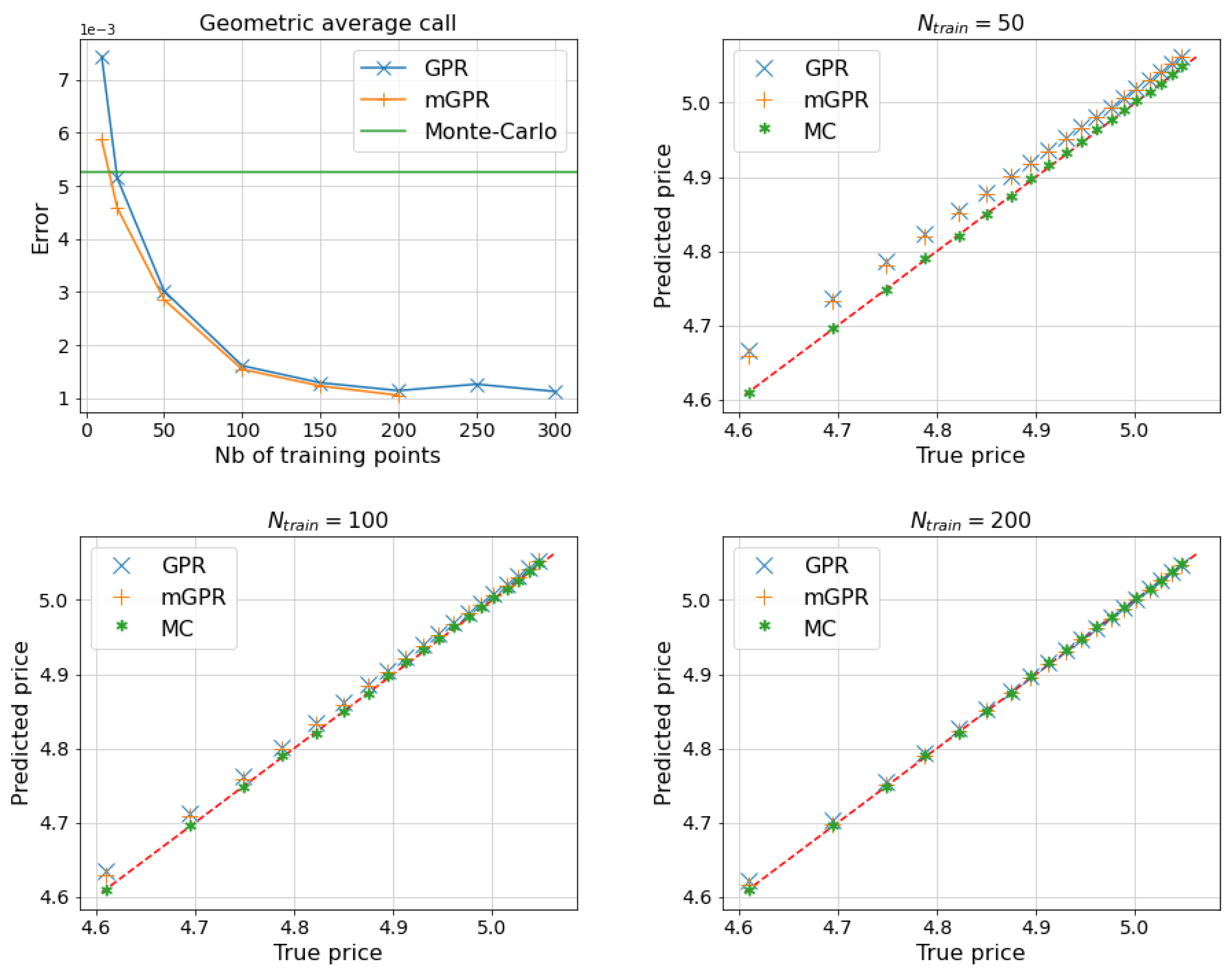
Figure 7.
MAPE of estimates of 5-asset basket call as a function of the number of training points (Top Left) and q-q plots comparing predictors learned from 50 (Top Right), 100 (Bottom Left) and 200 (Bottom Right) points against the true price, i.e. Monte-Carlo price with paths, below their quantile levels.
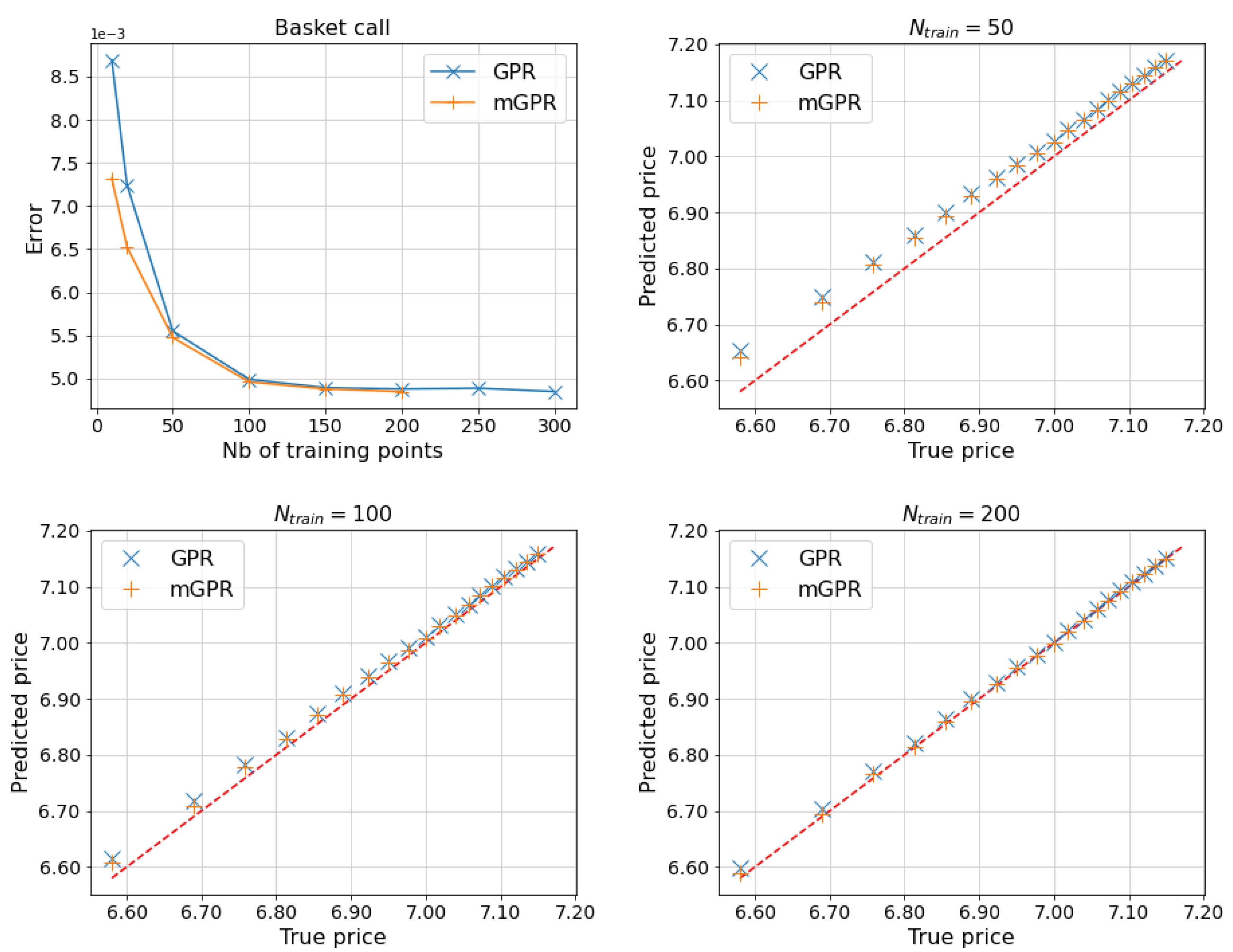
Figure 8.
MAPE of estimates of 5-asset best-of-call as a function of the number of training points (Top Left) and q-q plots comparing predictors learned from 50 (Top Right), 100 (Bottom Left) and 200 (Bottom Right) points against the true price, i.e. Monte-Carlo price with paths, below their quantile levels.
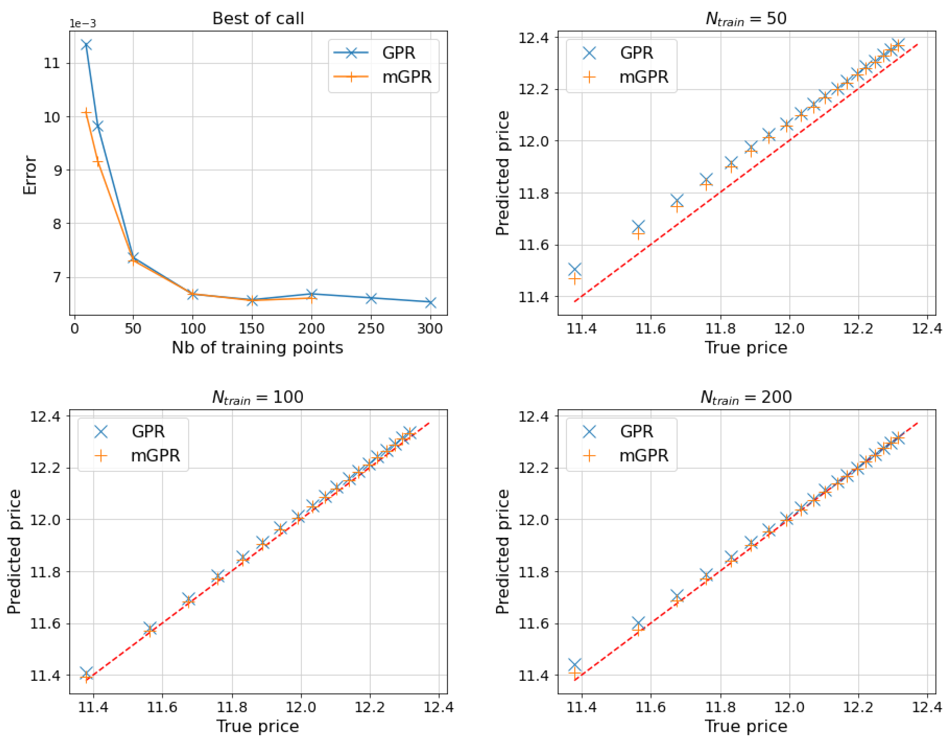
Figure 9.
MAPE of estimates of 5-asset worst-of call as a function of the number of training points (Top Left) and q-q plots comparing predictors learned from 50 (Top Right), 100 (Bottom Left) and 200 (Bottom Right) points against the true price, i.e. Monte-Carlo price with paths, below their quantile levels.
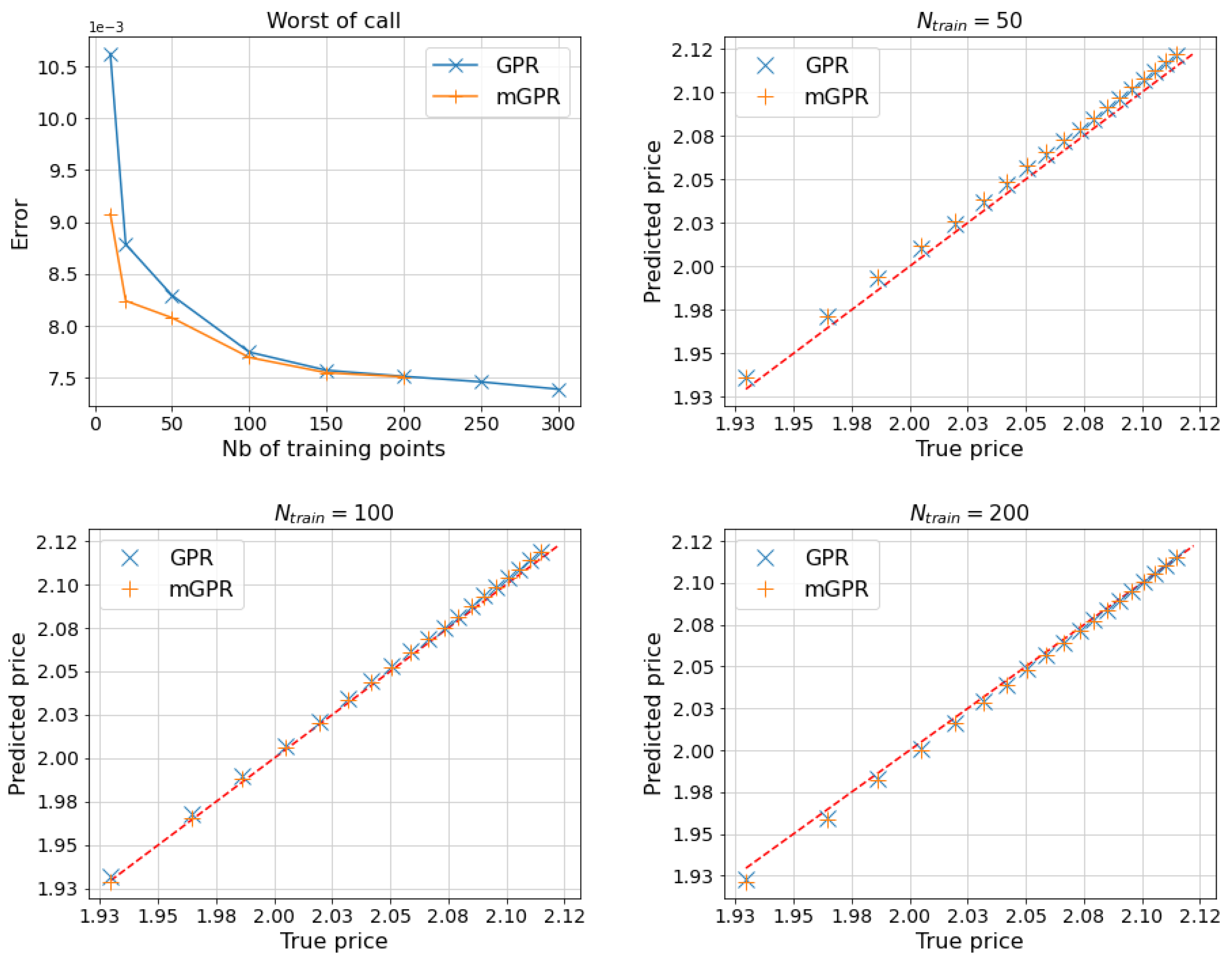
Figure 10.
MAPE of estimates of equity option portfolio with one day horizon as a function of the number of training points (Top Left) and q-q plots comparing predictors learned from 40 (Top Right), 100 (Bottom Left) and 500 (Bottom Right) points against the true price, i.e. Monte-Carlo price with paths, below their quantile levels. The MAPE of SxS prediction is not included in figures due to its high value but can be found in Table 9.

Figure 11.
MAPE of estimates of equity option portfolio with ten days horizon as a function of the number of training points (Top Left) and q-q plots comparing predictors learned from 40 (Top Right), 100 (Bottom Left) and 500 (Bottom Right) points against the true price, below their quantile levels. The MAPE of SxS prediction is not included in figures due to its high value but can be found in Table 11.
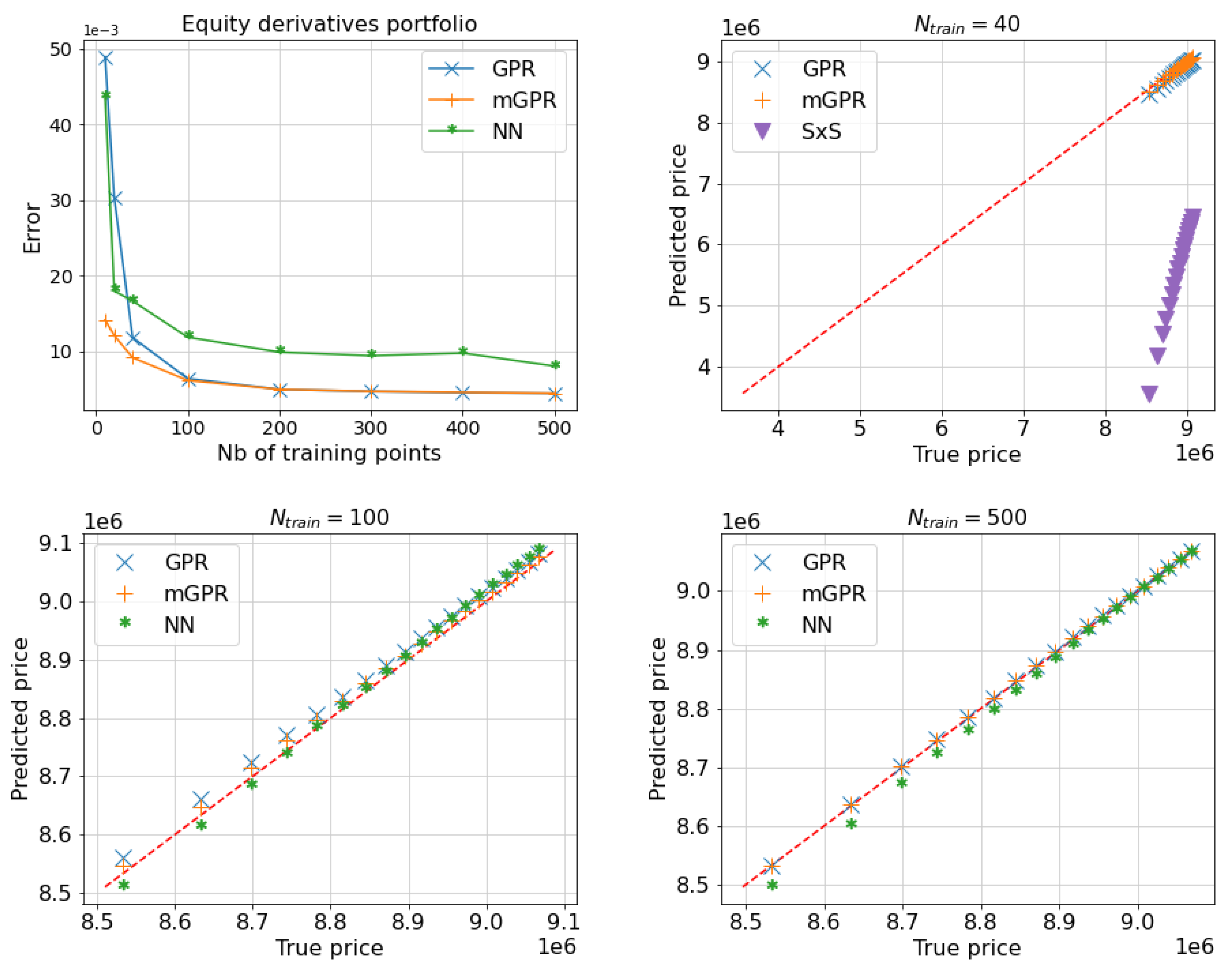
Figure 12.
MAPE of estimates of equity option portfolio with one month horizon as a function of the number of training points (Top Left) and q-q plots comparing predictors learned from 40 (Top Right), 100 (Bottom Left) and 500 (Bottom Right) points against the true price, i.e. Monte-Carlo price with paths, below their quantile levels. The MAPE of SxS prediction is not included in figures due to its high value but can be found in Table 12.
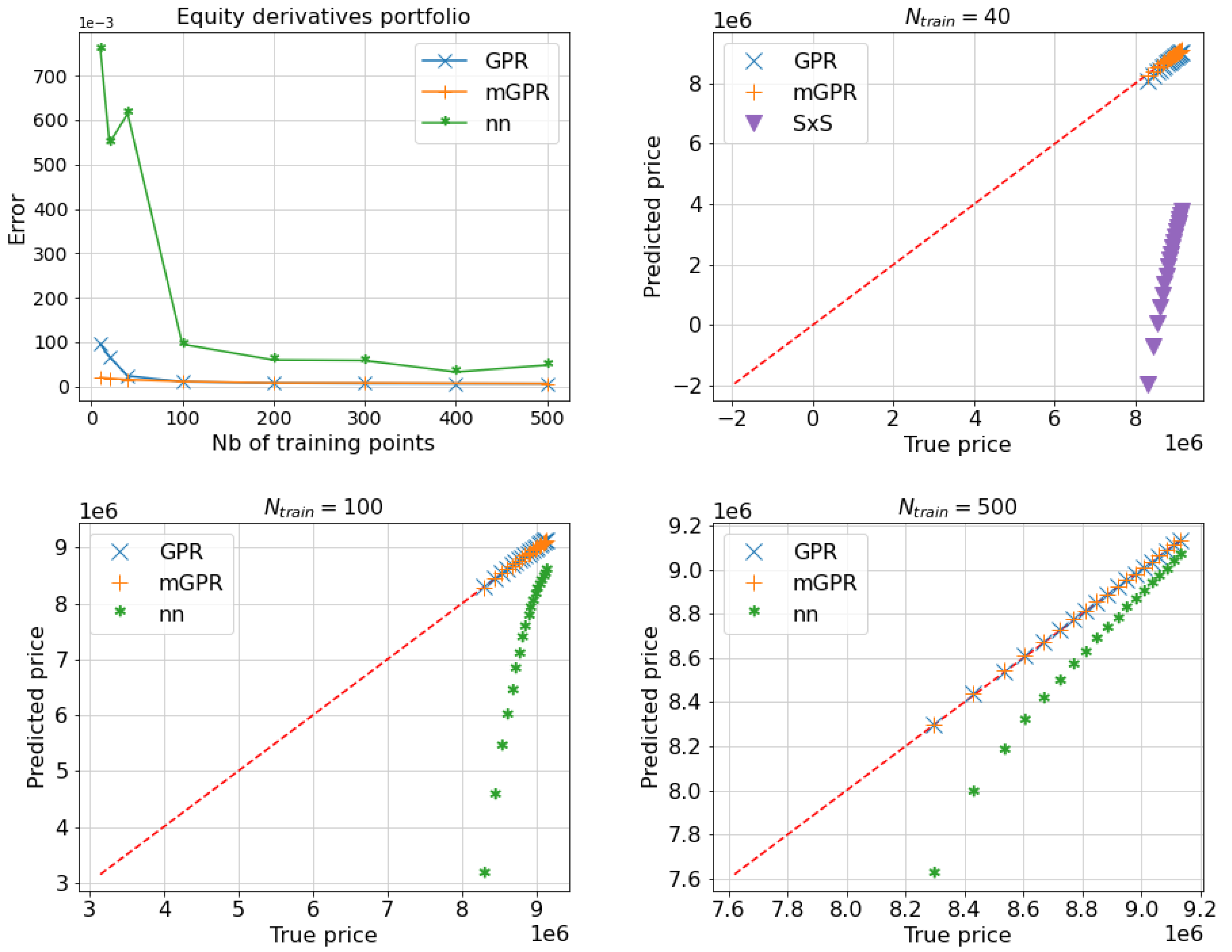
Figure A1.
Two-hidden-layer neural network architecture.
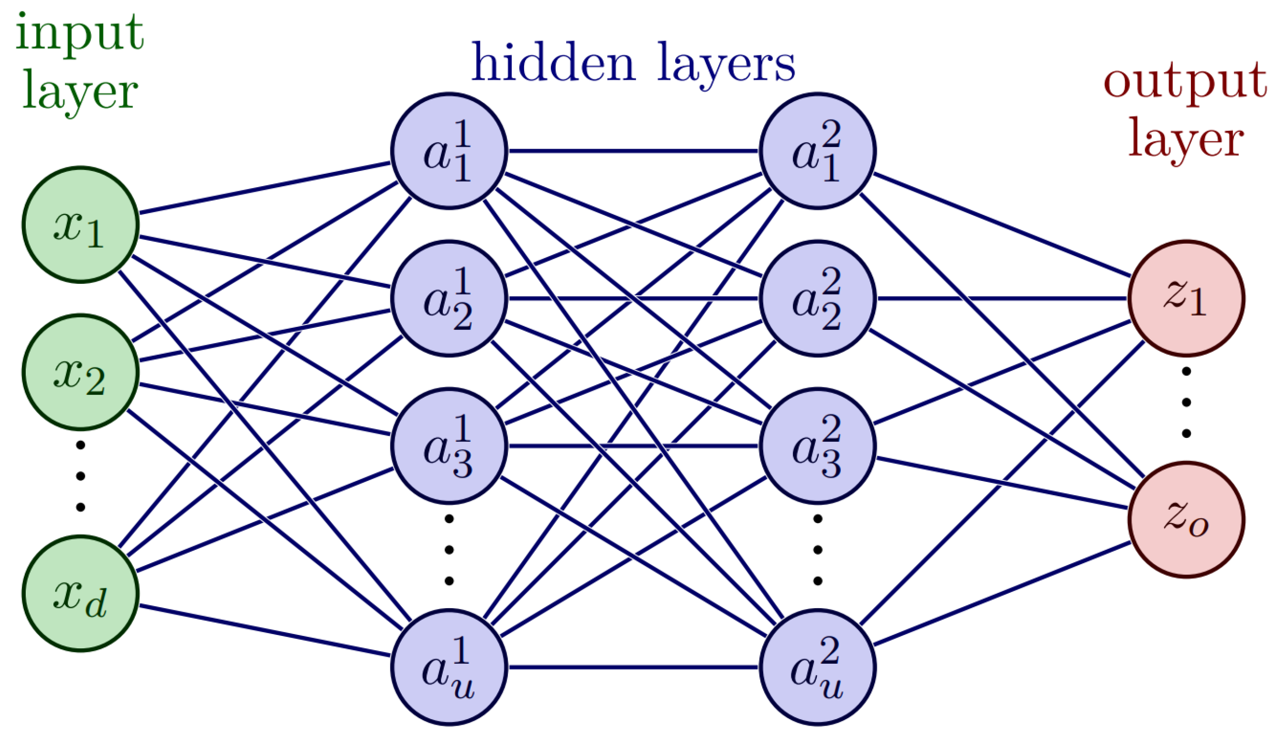

Table 1.
Multi-asset options covered in our numerics.
| Option | Geometric average call/put |
Basket call/put | Best-of call/put |
Worst-of call/put |
|---|---|---|---|---|
| Payoff |
with . The case , for , defines arithmetic average options.
Table 2.
Out-of-sample mean absolute error (MAE) of the predictors against the American put price computed by binomial tree of 100 time steps. The GPR with control variate learns the discrepancy between American price and its European counterpart. The BW approximation refers to the [2] approach.
Table 2.
Out-of-sample mean absolute error (MAE) of the predictors against the American put price computed by binomial tree of 100 time steps. The GPR with control variate learns the discrepancy between American price and its European counterpart. The BW approximation refers to the [2] approach.
| Model | GPR | GPR with control variate |
BW approximation |
mGPR |
|---|---|---|---|---|
| MAE | 0.6848 | 0.3199 | 0.2859 | 0.1367 |
Table 3.
Initial stock prices.
| 103.79 | 115.33 | ||
|---|---|---|---|
| 100.41 | 102.28 | ||
| 109.73 | 118.77 | ||
| 115.22 | 118 | ||
| 108.82 | 103.47 | ||
| 110.19 | 113.28 | ||
| 100.27 | 100.43 | ||
| 110.23 | 102.45 | ||
| 119.78 | 106.64 | ||
| 117.87 | 103.32 |
Table 4.
VaR and ES estimates using GPR against the true measures in the mono-asset portfolio case.
| Confidence level | True measure | ||||
|---|---|---|---|---|---|
| VaR | 39.83 | 39.84 | 39.83 | 39.83 | |
| 50.90 | 50.89 | 50.92 | 50.91 | ||
| 60.28 | 60.29 | 60.29 | 60.29 | ||
| 70.53 | 70.55 | 70.56 | 70.54 | ||
| ES | 53.98 | 53.98 | 53.99 | 53.98 | |
| 63.02 | 63.02 | 63.03 | 63.02 | ||
| 70.95 | 70.95 | 70.97 | 70.96 | ||
| 80.15 | 80.15 | 80.17 | 80.15 | ||
| Speed-up | 2h25 - benchmark | x2000 | x1000 | x500 |
Table 5.
One day and of 5-asset geometric average call estimated by proxy pricing models.
| Model | Number of training points () | ||||||
| 10 | 20 | 50 | 100 | 150 | 200 | ||
| VaR 99% |
GPR | 0.6900 | 0.7639 | 0.7768 | 0.8007 | 0.7989 | 0.8108 |
| mGPR | 0.7749 | 0.8028 | 0.7815 | 0.8054 | 0.8018 | 0.8155 | |
| MC | 0.8220 | ||||||
| True | 0.8190 | ||||||
| ES 97.5% |
GPR | 0.6931 | 0.7650 | 0.7757 | 0.8011 | 0.8005 | 0.8108 |
| mGPR | 0.7781 | 0.8060 | 0.7811 | 0.8057 | 0.8033 | 0.8159 | |
| MC | 0.8235 | ||||||
| True | 0.8202 | ||||||
| Computational time (in second) |
GPR | 0 | 1 | 3 | 6 | 10 | 13 |
| mGPR | 10 | 10 | 12 | 23 | 30 | 32 | |
| MC | 7488 | ||||||
| True initial price | 5.5135 | ||||||
Table 6.
One day and of 5-asset basket call estimated by proxy pricing models.
| Model | Number of training points () | ||||||
| 10 | 20 | 50 | 100 | 150 | 200 | ||
| VaR 99% |
GPR | 0.9163 | 1.0067 | 1.0289 | 1.0597 | 1.0588 | 1.0732 |
| mGPR | 1.0123 | 1.0550 | 1.0371 | 1.0673 | 1.0630 | 1.0824 | |
| True | 1.1013 | ||||||
| ES 97.5% |
GPR | 0.9199 | 1.0077 | 1.0280 | 1.0615 | 1.0607 | 1.0748 |
| mGPR | 1.0143 | 1.0583 | 1.0371 | 1.0674 | 1.0643 | 1.0832 | |
| True | 1.1016 | ||||||
| True initial price | 7.7770 | ||||||
Table 7.
One day and of 5-asset best-of-call estimated by proxy pricing models.
| Model | Number of training points () | ||||||
| 10 | 20 | 50 | 100 | 150 | 200 | ||
| VaR 99% |
GPR | 1.4704 | 1.5850 | 1.6380 | 1.7258 | 1.6907 | 1.7064 |
| mGPR | 1.5869 | 1.6604 | 1.6682 | 1.7403 | 1.6982 | 1.7346 | |
| True | 1.7483 | ||||||
| ES 97.5% |
GPR | 1.4714 | 1.5878 | 1.6435 | 1.7279 | 1.6928 | 1.7084 |
| mGPR | 1.5906 | 1.6675 | 1.6721 | 1.7438 | 1.7010 | 1.7373 | |
| True | 1.7517 | ||||||
| True initial price | 13.3101 | ||||||
Table 8.
One day and of 5-asset worst-of call estimated by proxy pricing models.
| Model | Number of training points () | ||||||
| 10 | 20 | 50 | 100 | 150 | 200 | ||
| VaR 99% |
GPR | 0.3153 | 0.3447 | 0.3584 | 0.3619 | 0.3661 | 0.3704 |
| mGPR | 0.3625 | 0.3673 | 0.3584 | 0.3640 | 0.3677 | 0.3711 | |
| True | 0.3651 | ||||||
| ES 97.5% |
GPR | 0.3625 | 0.3673 | 0.3584 | 0.3640 | 0.3677 | 0.3711 |
| mGPR | 0.3624 | 0.3670 | 0.3587 | 0.3645 | 0.3681 | 0.3715 | |
| True | 0.3657 | ||||||
| True initial price | 2.3296 | ||||||
Table 9.
Pricing approximation and risk calculation of the portfolio with one day horizon.
| Full pricing |
40 | 100 | 500 | |||||||
|---|---|---|---|---|---|---|---|---|---|---|
| model | SxS | GPR | mGPR | NN | GPR | mGPR | NN | GPR | mGPR | |
| MAPE | 9,447,616 | 6.13% | 0.61% | 0.57% | 0.48% | 0.43% | 0.42% | 0.43% | 0.38% | 0.38% |
| 358,862 | 1,575,039 | 307,983 | 325,145 | 374,986 | 340,394 | 343,926 | 368,887 | 350,397 | 351,493 | |
| 359,972 | 1,584,907 | 309,301 | 328,193 | 377,288 | 342,130 | 347,312 | 370,475 | 351,211 | 353,116 | |
| Err. | - | 12.87% | 0.54% | 0.36% | 0.17% | 0.20% | 0.16% | 0.11% | 0.09% | 0.08% |
| Err. | - | 12.97% | 0.54% | 0.34% | 0.18% | 0.19% | 0.13% | 0.11% | 0.09% | 0.07% |
Table 10.
Computation time comparison of and calculation by alternative methods.
| Full valorisation |
40 | 100 | 500 | |||||||
|---|---|---|---|---|---|---|---|---|---|---|
| model | SxS | GPR | mGPR | NN | GPR | mGPR | NN | GPR | mGPR | |
| Learning time | 0 | 0 | 1 | 41 | 25 | 2 | 56 | 30 | 13 | 135 |
| Sampling time | 600 | 0.2 | 0.6 | 3 | ||||||
Table 11.
Pricing approximation and risk calculation of the portfolio with ten days horizon.
| Full pricing |
40 | 100 | 500 | |||||||
|---|---|---|---|---|---|---|---|---|---|---|
| model | SxS | GPR | mGPR | NN | GPR | mGPR | NN | GPR | mGPR | |
| MAPE | 9,447,616 | 20.27% | 1.18% | 0.92% | 1.19% | 0.64% | 0.61% | 0.8% | 0.44% | 0.44% |
| 814,166 | 5,252,412 | 896,191 | 843,186 | 835,971 | 785,850 | 799,501 | 847,257 | 810,857 | 811,540 | |
| 814,604 | 5,320,871 | 895,574 | 843,831 | 836,584 | 787,204 | 800,163 | 848,514 | 812,423 | 812,947 | |
| Err. | - | 46.98% | 0.87% | 0.31% | 0.23% | 0.30% | 0.16% | 0.35% | 0.04% | 0.03% |
| Err. | - | 47.70% | 0.86% | 0.31% | 0.23% | 0.29% | 0.15% | 0.36% | 0.02% | 0.02% |
Table 12.
Pricing approximation and risk calculation of the portfolio with one month horizon.
| Full pricing |
40 | 100 | 500 | |||||||
|---|---|---|---|---|---|---|---|---|---|---|
| model | SxS | GPR | mGPR | NN | GPR | mGPR | NN | GPR | mGPR | |
| MAPE | 9,447,616 | 38.44% | 2.35% | 1.50% | 9.48% | 1.02% | 1.09% | 1.72% | 0.60% | 0.60% |
| 1,016,862 | 10,137,189 | 1,175,837 | 1,046,029 | 1,092,622 | 995,794 | 1,006,735 | 1,103,964 | 1,009,737 | 1,010,166 | |
| 1,011,890 | 10,267,028 | 1,177,443 | 1,042,407 | 1,104,343 | 991,431 | 1,004,123 | 1,119,376 | 1,005,141 | 1,005,065 | |
| Err. | 96.54% | 1.68% | 0.31% | 0.8% | 0.22% | 0.11% | 0.92% | 0.08% | 0.07% | |
| Err. | 97.96% | 1.75% | 0.32% | 0.98% | 0.22% | 0.08% | 1.14% | 0.07% | 0.07% | |
Disclaimer/Publisher’s Note: The statements, opinions and data contained in all publications are solely those of the individual author(s) and contributor(s) and not of MDPI and/or the editor(s). MDPI and/or the editor(s) disclaim responsibility for any injury to people or property resulting from any ideas, methods, instructions or products referred to in the content. |
© 2025 by the authors. Licensee MDPI, Basel, Switzerland. This article is an open access article distributed under the terms and conditions of the Creative Commons Attribution (CC BY) license (http://creativecommons.org/licenses/by/4.0/).
Copyright: This open access article is published under a Creative Commons CC BY 4.0 license, which permit the free download, distribution, and reuse, provided that the author and preprint are cited in any reuse.


