Preprint
Review

Deep Learning in Airborne Particulate Matter sensing and Surface Plasmon Resonance for Environmental Monitoring

This version is not peer-reviewed.

Submitted:

11 March 2025

Posted:

13 March 2025

You are already at the latest version

Abstract

This review explores advanced sensing technologies and Deep Learning (DL) methodologies for monitoring airborne particulate matter (PM), critical for environmental health assessment. It begins with discussing the significance of PM monitoring and introduces surface plasmon resonance (SPR) as a promising technique in environmental applications, alongside the role of DL neural networks in enhancing these technologies. This review analyzes advancements in airborne PM sensing technologies and the integration of DL methodologies for environmental monitoring. The review emphasizes the importance of PM monitoring for public health, environmental policy, and scientific research. Traditional PM sensing methods, including their principles, advantages, and limitations, are discussed, covering gravimetric techniques, continuous monitoring, optical and electrical methods, and microscopy. The integration of DL with PM sensing offers potential for enhancing monitoring accuracy, efficiency, and data interpretation. DL techniques such as convolutional neural networks (CNNs), autoencoders, recurrent neural networks (RNNs), and their variants, are examined for applications like PM estimation from satellite data, air quality prediction, and sensor calibration. The review highlights data acquisition and quality challenges in developing effective DL models for air quality monitoring. Techniques for handling large and noisy datasets are explored, emphasizing the importance of data quality for model performance, generalizability, and interpretability. The emergence of low-cost sensor technologies and hybrid systems for PM monitoring is discussed, acknowledging their promise while recognizing the need for addressing data quality, standardization, and integration issues. The review identifies areas for future research, including the development of robust DL models, advanced data fusion techniques, applications of deep reinforcement learning, and considerations of ethical implications.

Keywords: 
;  ;  ;  ;  ;  ;  ;  

1. Introduction:

Airborne PM is a complex mixture of solid particles and liquid droplets suspended in the air, varying in size, composition, and origin. Monitoring PM has become increasingly crucial due to its profound impacts on human health, environmental safety, and climate change. The significance of PM monitoring spans several key areas, including public health protection, environmental preservation, and policy development. From a public health perspective, PM monitoring is vital due to the severe health impacts associated with exposure. The World Health Organization (WHO) estimates that exposure to fine PM (PM2.5) contributes to approximately 4.2 million premature deaths globally each year, primarily due to cardiovascular and respiratory diseases, and lung cancer[1]. PM, especially fine (PM2.5) and ultrafine particles, can penetrate deep into the respiratory system and even enter the bloodstream, leading to a wide range of health problems[2].
Long-term exposure to PM has been associated with increased mortality rates, reduced life expectancy, and a higher incidence of chronic diseases such as asthma, chronic obstructive pulmonary disease (COPD), and cardiovascular disorders. Short-term exposure to high levels of PM can exacerbate existing health conditions and lead to acute health effects, including increased hospital admissions for respiratory and cardiovascular issues[3]. Children, the elderly, and individuals with pre-existing health conditions are particularly vulnerable to the adverse effects of PM exposure. Recent studies have also suggested potential links between PM exposure and neurological disorders, including cognitive decline and an increased risk of dementia[4]. Given the wide-ranging health impacts, accurate monitoring of PM levels is essential for assessing public health risks and implementing timely interventions to protect vulnerable populations .
From an environmental perspective, PM monitoring is crucial for understanding and mitigating its impacts on ecosystems and climate. Different components of PM can have varying effects on climate. While some particles, such as black carbon, contribute to global warming by absorbing solar radiation, others, like sulfates, have a cooling effect by reflecting sunlight back into space [5]. Understanding the composition and distribution of PM through comprehensive monitoring is essential for accurate climate modeling and prediction.
PM deposition can harm plant life by blocking stomata, reducing photosynthesis, and altering soil chemistry. This can lead to reduced agricultural productivity and changes in ecosystem composition[6]. Furthermore, PM can be deposited in water bodies, affecting aquatic ecosystems and potentially contaminating drinking water sources [7]. Fine particles are also the primary cause of reduced visibility in many urban and natural areas, including national parks and wilderness areas[8]. From a regulatory and policy standpoint, effective monitoring of PM is essential for developing and enforcing air quality standards and regulations. Many countries and international organizations have established air quality guidelines and standards based on PM concentrations. For instance, the United States Environmental Protection Agency (EPA) has set National Ambient Air Quality Standards (NAAQS) for PM2.5 and PM10, which require regular monitoring and reporting[9]. Accurate PM monitoring data is crucial for assessing compliance with air quality standards, identifying pollution hotspots and sources, evaluating the effectiveness of air pollution control measures, informing urban planning and zoning decisions, and providing timely public health advisories during high pollution events. This information is vital for policymakers to develop and implement effective strategies for reducing PM pollution and its associated health and environmental impacts.
Recent technological advancements have significantly improved our ability to monitor PM accurately and in real-time. Traditional monitoring methods, such as gravimetric analysis, are being complemented and sometimes replaced by more advanced techniques. These include optical particle counters, satellite remote sensing, low-cost sensors, and the application of machine learning and artificial intelligence for data analysis and forecasting[10]. The development of affordable, portable PM sensors has enabled the creation of dense monitoring networks and citizen science initiatives, greatly increasing the spatial resolution of PM data. This enhanced monitoring capability allows for more comprehensive and detailed assessments of PM distribution and its impacts on local communities. As urbanization continues and climate change alters atmospheric dynamics, the need for accurate, comprehensive PM monitoring will only increase. Future directions in PM monitoring include improving the characterization of PM composition and sources, better understanding the health effects of ultrafine particles and specific PM components, developing more accurate exposure assessment methods, and integrating PM monitoring with other environmental and health data for comprehensive risk assessment. Additionally, there is a growing focus on addressing environmental justice concerns related to disproportionate PM exposure in disadvantaged communities. Improved monitoring can help identify and address these disparities, ensuring that air quality management strategies benefit all populations equally.
Surface plasmon resonance (SPR) is a powerful and versatile optical sensing technique that has gained significant attention in the field of environmental monitoring. SPR is based on the excitation of surface plasmons-coherent electron oscillations that exist at the interface between a metal and a dielectric material-by incident light. This phenomenon is highly sensitive to changes in the refractive index near the metal surface, making SPR an excellent tool for detecting and quantifying various environmental contaminants and changes in environmental conditions. The fundamental principle of SPR involves the interaction of light with free electrons on a metal surface, typically gold or silver, which results in a reduction in the intensity of reflected light at a specific angle or wavelength. This change is highly sensitive to the adsorption of molecules on the metal surface, as it alters the local refractive index. As such, SPR can be used to monitor the presence of pollutants, such as heavy metals, pesticides, and other hazardous substances, in air, water, and soil environments. The ability to provide real-time, label-free detection makes SPR an attractive option for continuous environmental monitoring applications [11, 12].
One of the key advantages of SPR in environmental monitoring is its high sensitivity and specificity. SPR sensors can detect minute changes in the refractive index, allowing for the detection of low concentrations of pollutants. This sensitivity is further enhanced by the use of nanomaterials, such as graphene and gold nanoparticles, which amplify the SPR signal and improve detection limits. For example, SPR sensors have been developed to detect heavy metals like cadmium and lead in water samples, demonstrating the potential for these sensors to provide early warning of contamination events [13]. Additionally, SPR can be integrated with other sensing technologies, such as fiber optics, to create compact and portable devices suitable for field deployment [14]. The versatility of SPR extends beyond chemical detection to include biological monitoring. SPR can be used to detect pathogens, allergens, and other biological agents in the environment, which is particularly important for monitoring water quality and ensuring the safety of drinking water supplies. SPR-based biosensors can detect specific proteins, nucleic acids, and microorganisms by exploiting the specific binding interactions between target molecules and immobilized biorecognition elements on the sensor surface. This capability allows for the rapid and accurate detection of biological contaminants, which is crucial for preventing the spread of diseases and protecting public health [15].
Moreover, SPR technology is continually evolving, with recent advances focusing on enhancing its performance and expanding its applications. Innovations such as the development of SPR imaging (SPRI) and the integration of SPR with smartphone technology have opened new possibilities for environmental monitoring. SPRI allows for the visualization of spatial distributions of analytes on the sensor surface, providing additional information about the sample composition and enabling multiplexed detection of multiple analytes simultaneously. Meanwhile, smartphone-based SPR platforms offer a cost-effective and accessible solution for on-site environmental monitoring, allowing users to perform analyses without the need for specialized laboratory equipment [16]. The application of SPR in environmental monitoring is not without challenges. The performance of SPR sensors can be affected by factors such as temperature fluctuations, non-specific binding, and matrix effects from complex environmental samples. To address these issues, ongoing research is focused on improving sensor design, developing robust surface chemistries, and implementing advanced data analysis techniques. For instance, the use of machine learning algorithms to process SPR data can enhance the accuracy and reliability of detection by compensating for environmental interferences and extracting meaningful patterns from complex datasets [14]. The surface plasmon resonance is a highly effective and adaptable tool for environmental monitoring, offering real-time, sensitive, and specific detection of a wide range of chemical and biological contaminants. Its ability to operate in diverse environmental settings and its potential for integration with modern technologies make SPR a promising approach for addressing current and future challenges in environmental health and safety. As research and development in this field continue to advance, SPR is expected to play an increasingly important role in safeguarding the environment and public health.
Despite the advantages, implementing SPR for environmental monitoring, particularly for airborne pollutants, presents several challenges: Environmental Interferences: Temperature fluctuations, humidity variations, and non-specific binding of molecules present in complex environmental samples can significantly affect the performance of SPR sensors. These interferences can lead to signal drift, reduced sensitivity, and inaccurate measurements, particularly for low concentrations of airborne pollutants. Matrix Effects: The composition of airborne particulate matter is highly diverse, with varying particle sizes, shapes, and chemical properties. These matrix effects can influence the interaction of pollutants with the SPR sensor surface, leading to measurement inconsistencies and difficulties in accurately quantifying specific pollutants. Sensitivity to Ultrafine Particles: Ultrafine particles, while posing significant health risks, contribute minimally to the overall mass of particulate matter. SPR sensors may have limitations in detecting and quantifying these ultrafine particles due to their small size and low mass, potentially underestimating their contribution to air pollution levels. Surface Chemistry and Functionalization: Developing robust and selective surface chemistries for SPR sensors is crucial for targeting specific airborne pollutants. Non-specific binding of other molecules present in the air can interfere with the detection of the target pollutant, reducing sensor accuracy and reliability. Real-Time Monitoring and Data Processing: Continuous, real-time monitoring of airborne pollutants using SPR requires efficient data acquisition and processing systems. The development of algorithms and software to handle the high data rates generated by SPR sensors and to compensate for environmental interferences is essential for reliable air quality monitoring. Cost and Portability: While SPR technology has advanced significantly, the cost and portability of SPR systems for widespread environmental monitoring remain considerations. Developing miniaturized, cost-effective SPR sensors that can be easily deployed in various environments is crucial for expanding the application of this technology for air quality assessment.

2. Airborne Particulate Mater Sensing:

Accurate measurement of PM concentrations is crucial for assessing air quality, understanding pollution sources, and evaluating potential health impacts. Over the years, various sensing techniques have been developed to quantify PM levels in the atmosphere. This section provides an overview of the traditional methods used for measuring airborne PM, their principles of operation, advantages, and limitations. EPA reference methods, such as the Federal Reference Method (FRM) and Federal Equivalent Methods (FEMs), are essential for providing accurate and reliable PM measurements for regulatory purposes. These methods, typically based on gravimetric analysis, establish a baseline for evaluating the performance of other PM sensing technologies. While fundamental to air quality monitoring, EPA reference methods often involve time-intensive sampling and analysis procedures, which can limit their spatial and temporal coverage. The conventional methods of PM sensing are shown in the figure 1, and they are breifely described in the following subsections as well.

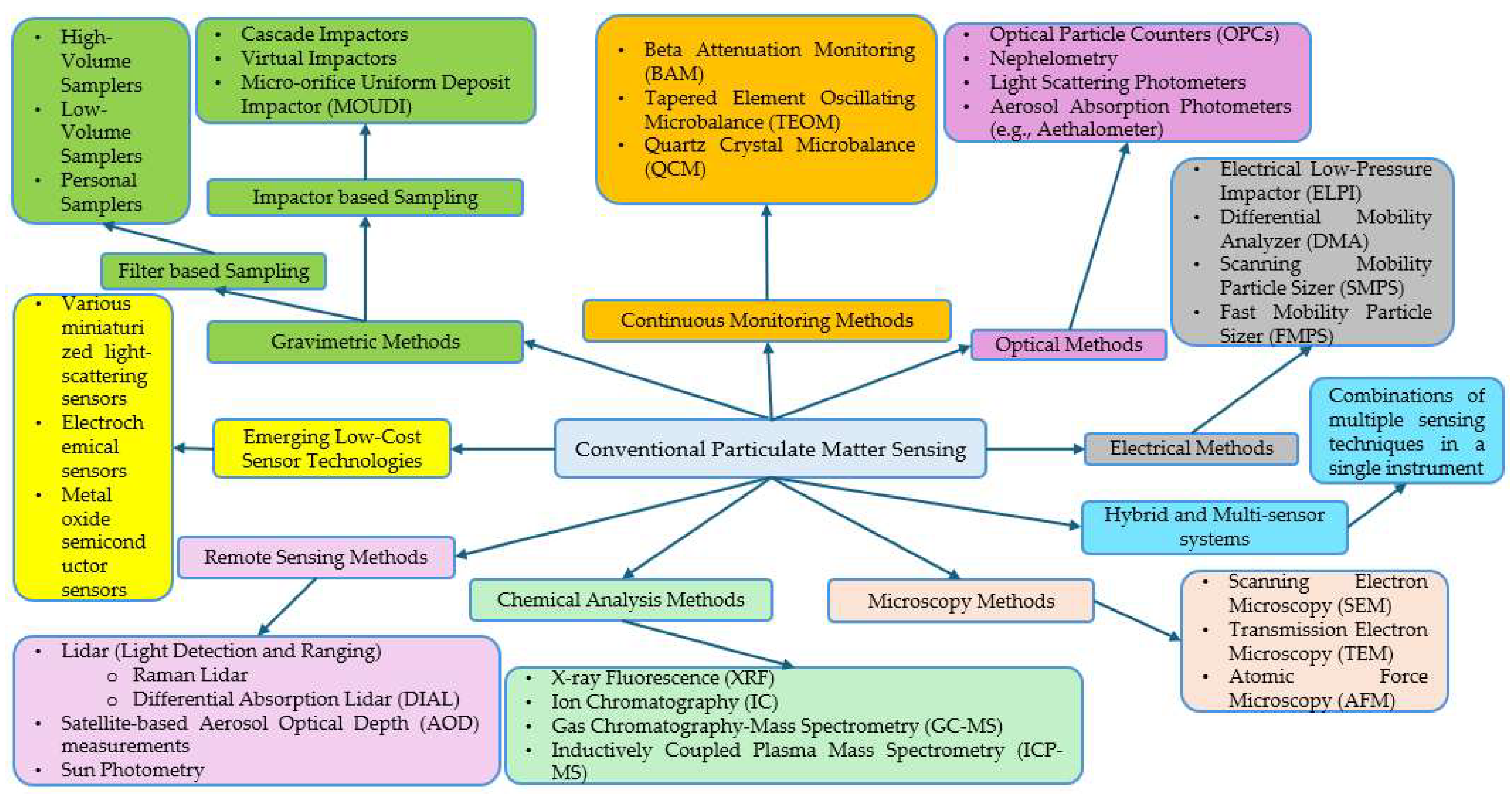
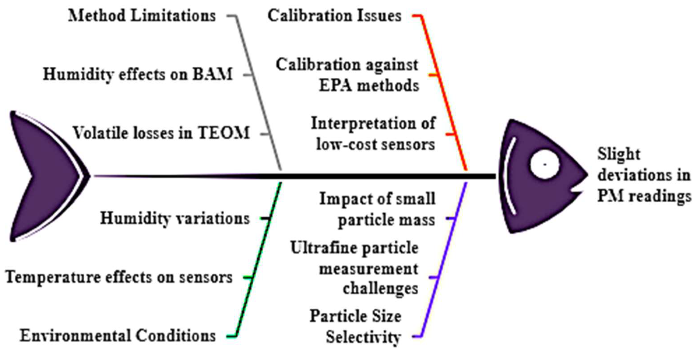
2.1 Traditional methods of measuring airborne PM, and their limitations and challenges

Various traditional methods are employed for particulate matter (PM) sensing, each relying on different principles and offering unique advantages and limitations. As shown in Figure 1, these conventional methods encompass a range of techniques, including: Gravimetric methods, which rely on mass measurements. Continuous monitoring techniques, such as the Tapered Element Oscillating Microbalance (TEOM) and Beta Attenuation Monitoring (BAM). Optical methods, which measure light scattering or absorption by particles . Electrical methods, such as the Electrical Low Pressure Impactor (ELPI) and Scanning Mobility Particle Sizer (SMPS). Microscopy methods, including Scanning Electron Microscopy (SEM) and Transmission Electron Microscopy (TEM). The following subsections will delve into each of these methods, detailing their principles of operation, benefits, and drawbacks.

2.1.1. Gravimetric Methods

Gravimetric methods of sampling are fundamental techniques in the field of air quality monitoring and PM analysis. These methods rely on the principle of mass measurement to quantify the concentration of airborne particles. Filter-based sampling, which includes high-volume, low-volume, and personal samplers, is the most common gravimetric approach. High-volume samplers, such as those used by Chow et al. (2006), typically operate at flow rates of 1.13 to 1.70 m³/min and are primarily used for measuring total suspended particles (TSP) and PM10[17]. Low-volume samplers, operating at lower flow rates (e.g., 16.7 L/min), are commonly employed for PM2.5 and PM10 measurements, as demonstrated in the study by Solomon et al. (2014)[18]. Personal samplers, designed for individual exposure assessment, have been effectively utilized by Brouwer et al. (2009) to evaluate occupational exposure to PM in various workplace environments[19]. These filter-based methods have proven invaluable in regulatory compliance monitoring and epidemiological studies due to their ability to provide accurate mass concentration data and allow for subsequent chemical analysis of collected particles.
Impactor-based gravimetric methods offer size-selective particle collection, enabling researchers to analyze the size distribution of airborne particulates. Cascade impactors, such as those employed by Marple et al. (1991), consist of multiple stages that separate particles based on their aerodynamic diameter, providing detailed information on particle size fractions[20]. Virtual impactors, as used in the study by Sioutas et al. (1994), utilize a unique design to separate particles into two size fractions without the need for impaction plates, reducing particle bounce and re-entrainment issues[21]. The Micro-orifice Uniform Deposit Impactor (MOUDI), developed by Marple et al. (1991) and utilized in numerous studies including that of Cass et al. (2000), offers high-resolution particle size separation with uniform particle deposition, making it particularly useful for chemical speciation studies[20, 22]. These impactor-based methods have been instrumental in understanding the size-dependent composition and behavior of atmospheric aerosols, contributing significantly to our knowledge of PM sources, formation mechanisms, and potential health impacts.
Despite their widespread use and reliability, gravimetric methods for measuring airborne PM face several limitations and challenges. One significant issue is the time-intensive nature of these techniques, as noted by Chow et al. (2006), which can delay the availability of data for timely decision-making in air quality management[23]. The potential for measurement artifacts due to volatile organic compounds and water absorption on filters, as highlighted by Vecchi et al. (2009), can lead to overestimation or underestimation of particle mass[24]. Sioutas et al. (1994) pointed out that impactor-based methods may suffer from particle bounce and re-entrainment, particularly for dry particles, potentially affecting size distribution measurements[21]. Additionally, gravimetric methods typically provide integrated measurements over extended sampling periods, limiting their ability to capture short-term fluctuations in PM concentrations, as discussed by Wilson et al. (2002)[25]. The labor-intensive nature of filter handling, conditioning, and weighing processes also introduces the potential for human error, as emphasized by Amaral et al. (2015) [26]. Furthermore, these methods generally do not provide real-time data, which can be crucial for immediate public health interventions during acute pollution events. Despite these limitations, gravimetric methods remain the gold standard for regulatory compliance monitoring due to their accuracy and traceability, as they align with EPA reference methods for PM measurement . These methods provide a direct measurement of particle mass, which is the primary metric used in EPA air quality standards. The established procedures and protocols for gravimetric sampling ensure consistency and comparability of measurements across different monitoring networks.

2.1.2. Continuous monitoring methods

Continuous monitoring methods for airborne PM have revolutionized air quality assessment by providing real-time, high-resolution data on particle concentrations. Among these methods, Beta Attenuation Monitoring (BAM), Tapered Element Oscillating Microbalance (TEOM), and Quartz Crystal Microbalance (QCM) have emerged as widely adopted techniques. BAM, which utilizes the attenuation of beta radiation by collected particles to determine mass concentration, has been extensively used in regulatory monitoring networks. For instance, Liu et al. (2023) employed BAM monitors to assess PM2.5 concentrations in urban areas of China, demonstrating its effectiveness in capturing diurnal and seasonal variations in PM levels[27]. The TEOM method, based on the change in oscillation frequency of a tapered element as particles accumulate, has been particularly valuable for continuous PM2.5 monitoring. In a comprehensive study, Su et al. (2021) compared TEOM measurements with filter-based methods, highlighting TEOM's ability to provide accurate, real-time data while minimizing volatilization losses[28]. The QCM technique, which measures mass loading through changes in the resonant frequency of a quartz crystal, has found applications in both outdoor and indoor air quality monitoring. Tariq et al. (2023) utilized QCM sensors for real-time monitoring of fine PM in indoor environments, showcasing its sensitivity and rapid response to concentration changes[29].
These continuous monitoring methods offer unique advantages over traditional gravimetric techniques. BAM provides excellent correlation with reference methods while offering continuous data collection, making it ideal for long-term monitoring programs. Jayaratne et al. (2020) demonstrated BAM's reliability in a year-long PM2.5 monitoring campaign across multiple urban sites[30]. TEOM's ability to provide highly time-resolved data has made it invaluable for studying short-term pollution events and their health impacts. For example, Yadav et al. (2022) used TEOM data to investigate the association between hourly PM2.5 concentrations and hospital admissions, revealing important insights into acute health effects of PM exposure[31]. QCM's high sensitivity to ultra-fine particles and rapid response time make it particularly suited for monitoring in dynamic environments or for tracking rapid changes in particle concentrations.
While these continuous monitoring methods offer significant advantages, they are not without limitations and challenges. Schweizer et al. (2016) highlighted the importance of understanding data and equipment limitations when using BAM for creating PM2.5 air quality health advisories[32]. They found that BAM measurements can be affected by relative humidity, potentially leading to overestimation of particle concentrations under high humidity conditions. Grover et al. (2005) demonstrated that traditional TEOM measurements may underestimate PM concentrations due to the loss of volatile components[33]. Their study compared TEOM measurements with filter-based methods and showed that the Filter Dynamic Measurement System (FDMS) TEOM can provide more accurate measurements by accounting for these volatile losses. Wang et al. (2015) evaluated three low-cost particle sensors in laboratory conditions, examining their performance and calibration needs[34]. They found that these sensors can be affected by environmental factors such as temperature, highlighting the importance of proper calibration and understanding of sensor limitations for accurate PM measurements. Additionally, all these methods face challenges in accurately measuring ultrafine particles, which contribute little to mass but may have significant health impacts. Kuula et al. (2020) evaluated the particle-size selectivity of low-cost optical PM sensors in laboratory conditions[35]. Their study highlighted challenges in accurately measuring smaller particles, including ultrafine particles, with these sensors. This work emphasizes the need for careful interpretation of data from low-cost instruments when assessing the full spectrum of PM sizes, particularly for air quality monitoring applications[35]. The challenges in the continuous PM Monitoring methods are summarised in Figure 2.
Continuous monitoring methods offer advantages in terms of real-time data acquisition, enabling more timely responses to air quality changes. However, it's crucial to calibrate them against EPA reference methods to ensure accuracy and comparability. EPA has established guidelines and protocols for evaluating the performance of continuous PM monitors, ensuring their measurements are traceable to reference methods. This rigorous evaluation process ensures the reliability and regulatory acceptance of continuous monitoring data.

2.1.3. Optical methods

Optical methods for measuring PM have become increasingly attractive in air quality monitoring due to their ability to provide real-time, high-resolution data. These methods include Optical Particle Counters (OPCs), nephelometers, light scattering photometers, and aerosol absorption photometers like the Aethalometer.
Optical Particle Counters (OPCs) have been widely used for their ability to provide size-resolved particle number concentrations. For example, Kuula et al. (2020) evaluated the particle-size selectivity of low-cost OPCs in laboratory conditions, demonstrating their potential for widespread air quality monitoring[35]. Their study showed that OPCs can effectively measure particles in the PM2.5 and PM10 size ranges, though with some limitations in accuracy for the smallest particles. Nephelometers, which measure light scattering by aerosols, have been employed in both stationary and mobile monitoring setups. Magi et al. (2020) used a nephelometer alongside a beta attenuation monitor to evaluate PM2.5 concentrations in an urban setting, highlighting the nephelometer's ability to capture short-term variations in particle concentrations[36].
Light scattering photometers offer rapid response times and high sensitivity, making them suitable for detecting sudden changes in particle concentrations. Malings et al. (2020) conducted a long-term evaluation of low-cost light scattering sensors for fine particle mass monitoring, demonstrating their potential for large-scale deployment after appropriate calibration[37]. Aerosol absorption photometers, such as the Aethalometer, provide unique insights into black carbon concentrations. Drinovec et al. (2015) described a new Aethalometer model with improved performance, showcasing its ability to measure black carbon with finer time resolution and sensitivity[38].
These optical methods are unique in their ability to provide real-time data with high temporal resolution, which is crucial for understanding short-term variations in air quality and for public health interventions. While gravimetric methods remain the gold standard for regulatory purposes, they cannot match the temporal resolution of optical methods. Additionally, optical methods allow for more widespread and cost-effective monitoring networks, as demonstrated by the increasing use of low-cost sensors in citizen science projects and urban air quality studies.
However, optical methods for PM measurement also face several limitations and challenges. One significant issue is the dependence of light scattering on particle properties such as size, shape, and refractive index, which can lead to measurement biases. Crilley et al. (2018) demonstrated that relative humidity can significantly affect the performance of optical particle counters, potentially leading to overestimation of particle mass concentrations under high humidity conditions[39]. Another challenge is the difficulty in accurately measuring ultrafine particles, which contribute little to mass but may have significant health impacts. Wang et al. (2015) highlighted the limitations of low-cost optical sensors in detecting particles smaller than 0.3 μm, which can be a significant portion of urban aerosols[34]. Calibration remains a critical issue, as the response of optical instruments can vary depending on the composition and size distribution of aerosols. Zheng et al. (2018) showed that the performance of low-cost optical sensors can vary significantly across different environments, emphasizing the need for location-specific calibrations[40]. Additionally, Alfano et al. (2020) pointed out that most optical methods assume spherical particle geometry and a standard particle density, which may not accurately represent the diverse range of atmospheric aerosols[41]. Despite these challenges, ongoing research and technological advancements continue to improve the accuracy and reliability of optical methods for PM measurement. While optical methods offer advantages in real-time monitoring and size-resolved measurements, their accuracy can be influenced by particle composition, size distribution, and environmental factors. Calibration against EPA reference methods, such as FRM or FEMs, is essential for reliable PM measurements. EPA provides guidance on calibration procedures and performance criteria for optical PM sensors to ensure their measurements are consistent with regulatory requirements.

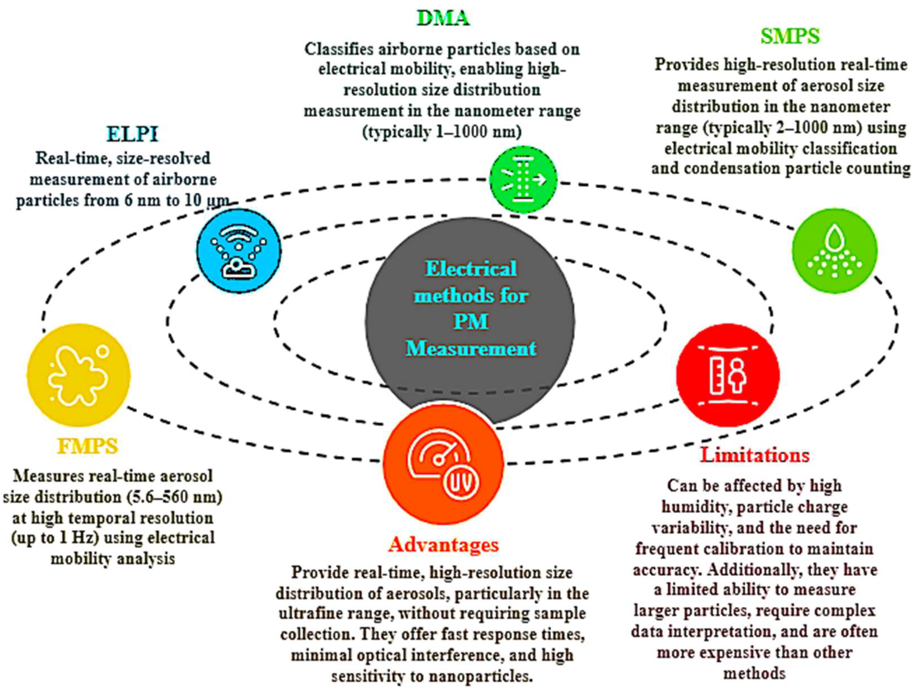
2.1.4. Electrical Methods:

Electrical methods for measuring airborne PM have become increasingly important in aerosol science due to their ability to provide high-resolution, real-time data on particle size distributions and concentrations. These methods include the Electrical Low Pressure Impactor (ELPI), Differential Mobility Analyzer (DMA), Scanning Mobility Particle Sizer (SMPS), and Fast Mobility Particle Sizer (FMPS), their overview is as shown in Figure 3.
The Electrical Low Pressure Impactor (ELPI) has gained popularity for its wide particle size range and real-time measurement capabilities. Lee et al. (2021) applied an ELPI to measure residual particles in an epitaxial growth reactor, demonstrating its effectiveness in monitoring chamber purge performance after semiconductor processing[42]. In a different application, Rissler et al. (2014) used ELPI to characterize nanoparticle emissions from a small-scale biomass combustion unit, highlighting its versatility in various emission studies[43].
The Differential Mobility Analyzer (DMA) and Scanning Mobility Particle Sizer (SMPS) are often used in tandem to provide high-resolution particle size distributions. Sowlat et al. (2016) employed an SMPS system to characterize ultrafine particles in urban environments, highlighting its capability to measure particles in the size range of 14.6 to 661.2 nm with high time resolution[44]. Their study in central Los Angeles demonstrated the SMPS's effectiveness in capturing detailed particle number size distributions, which were crucial for source apportionment of ambient particle number concentrations[44]. Similarly, Levin et al. (2014) utilized SMPS to investigate the size-resolved hygroscopicity of atmospheric aerosols, demonstrating its applicability in atmospheric science research[45].
The Fast Mobility Particle Sizer (FMPS) offers rapid measurements of particle size distributions, making it valuable for studying dynamic aerosol processes. Wang et al. (2015) utilized an FMPS to investigate the rapid changes in particle emissions during aircraft engine start-up and shutdown, demonstrating its unique ability to capture transient aerosol events with 1-second time resolution[34]. In another study, Zimmerman et al. (2014) used FMPS to characterize nanoparticle exposure during 3D printing processes, showcasing its applicability in occupational health research[46].
These electrical methods offer unique advantages over traditional optical or gravimetric techniques. They can measure particles in the nanometer range, which is crucial for understanding the formation and behavior of ultrafine particles that are of increasing concern in air quality and health studies. For instance, Fonseca et al. (2016) combined SMPS and ELPI measurements to characterize ultrafine particles in subway systems, demonstrating the complementary nature of these techniques in comprehensive aerosol characterization[47].
However, electrical methods for PM measurement also face several limitations and challenges. One significant issue is the potential for particle charging effects to influence measurements, particularly for ultrafine particles. Levin et al. (2015) demonstrated that the charging state of particles can affect their mobility and, consequently, their measured size distribution in electrical mobility analyzers[48]. Another challenge is the sensitivity of these instruments to changes in ambient conditions, such as temperature and humidity. Schmid et al. (2002) showed that relative humidity can significantly affect the performance of DMAs, potentially leading to measurement biases in atmospheric studies[49]. Additionally, these instruments often require a stable power supply and controlled environmental conditions, which can limit their applicability in field studies. Wu et al. (2013) highlighted the importance of careful instrument design and data processing when using SMPS systems in field measurements, emphasizing the need to account for factors such as particle hygroscopicity and chemical composition that can affect size distribution measurements[50]. Furthermore, the high cost and complexity of many electrical measurement systems can limit their widespread deployment, particularly in large-scale monitoring networks. Despite these challenges, ongoing research and technological advancements continue to improve the accuracy, reliability, and applicability of electrical methods for PM measurement in diverse environmental conditions.

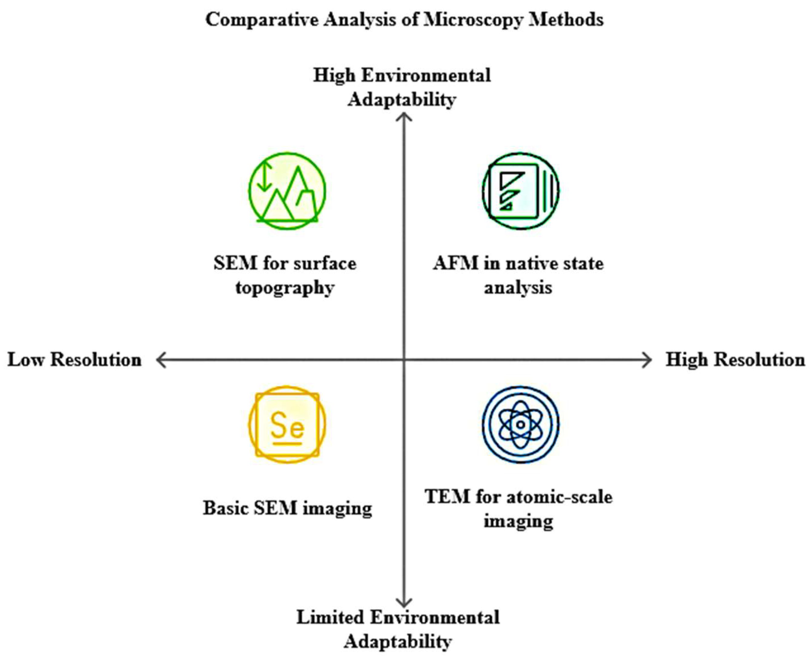
2.1.5. Microscopy methods

Microscopy methods such as Scanning Electron Microscopy (SEM), Transmission Electron Microscopy (TEM), and Atomic Force Microscopy (AFM) have revolutionized our ability to visualize and analyze materials at the nanoscale. The comparative view of these methods are given in the Figure 4. These techniques offer unique capabilities for characterizing the structure, morphology, and properties of a wide range of samples.
Scanning Electron Microscopy (SEM) provides high-resolution imaging of particle surface topography and composition. Shi et al. (2015) utilized SEM to investigate the morphology and adhesive properties of PM2.5 airborne pollutants, revealing intricate details of soot particles and their aggregation capabilities[51]. The ability of SEM to provide three-dimensional-like images with a large depth of field makes it invaluable for studying complex structures of atmospheric particles.
Transmission Electron Microscopy (TEM) offers even higher resolution than SEM, allowing for atomic-scale imaging and analysis of internal structures of airborne particles. Longyi et al. (2022) employed TEM to study the mixing states of individual atmospheric particles, providing crucial insights into their formation and transformation processes[52]. TEM's unique capability to provide both real-space imaging and electron diffraction patterns makes it indispensable for crystallographic studies and chemical composition analysis of atmospheric aerosols.
Atomic Force Microscopy (AFM) stands out for its ability to provide three-dimensional surface topography of airborne particles with sub-nanometer resolution. Shi et al. (2015) used AFM to investigate the nanoscale mechanical properties of PM2.5 particles, demonstrating its potential for characterizing the adhesiveness and deformation of airborne pollutants[51]. AFM's versatility in operating under various environmental conditions makes it particularly valuable for studying particles in their native state.
These microscopy methods are often used in combination to provide a comprehensive characterization of airborne PM. For instance, Sielicki et al. (2011) combined SEM and TEM with Energy-dispersive X-ray spectroscopy (EDX/EDS) to analyze metal-containing airborne particles, leveraging SEM for overall morphology and TEM for detailed internal structure and elemental composition[53].
Recent advancements in microscopy techniques have further expanded their capabilities in atmospheric particle analysis. Laskin et al. (2019) demonstrated the use of automated SEM/EDX for high-throughput characterization of thousands of individual particles, enabling statistically robust analysis of particle populations in complex atmospheric samples[54]. These microscopy methods complement traditional bulk analysis techniques by providing detailed information on individual particle characteristics, which is crucial for understanding the sources, transformation processes, and potential health impacts of airborne PM.
Despite their powerful capabilities, microscopy methods for analyzing airborne PM face several limitations and challenges. One significant issue is sample preparation, which can alter the original state of the particles. As noted by Ault and Axson (2017), the high vacuum environment required for SEM and TEM can cause volatile components to evaporate, potentially changing the particle morphology and composition[55]. AFM, while capable of operating in ambient conditions, faces challenges in accurately representing soft or sticky particles due to tip-sample interactions. Variola (2015) highlighted that while AFM provides high-resolution imaging of surface topography, it faces challenges in accurately representing soft or sticky particles due to tip-sample interactions[56]. The author also emphasized that the resolution of AFM is limited by the probe's geometry, which can lead to artifacts in imaging highly irregular particles. To address the challenge of analyzing large numbers of particles, Laskin et al. (2018) emphasized the need for automated, high-throughput analysis methods in atmospheric particle characterization using advanced mass spectrometry techniques[57]. Furthermore, the interpretation of microscopy data requires expertise and can be subjective, particularly for complex, heterogeneous atmospheric particles. Despite these challenges, ongoing advancements in instrumentation and data analysis techniques continue to enhance the applicability and reliability of microscopy methods in atmospheric PM research.

2.1.6. Chemical Analysis Methods

Chemical analysis methods play a crucial role in characterizing the composition of airborne PM. X-ray Fluorescence (XRF), Ion Chromatography (IC), Gas Chromatography-Mass Spectrometry (GC-MS), and Inductively Coupled Plasma Mass Spectrometry (ICP-MS) are widely used techniques for this purpose.
X-ray Fluorescence (XRF) is a non-destructive method that allows for rapid multi-elemental analysis of PM samples. Yatkin et al. (2012) demonstrated the effectiveness of XRF in analyzing elemental composition of PM2.5 samples collected on filters, highlighting its ability to detect a wide range of elements simultaneously[58]. The non-destructive nature of XRF makes it particularly valuable for preserving samples for further analysis.
Ion Chromatography (IC) is extensively used for the analysis of water-soluble ionic species in PM. Correa et al. (2023) reviewed various characterization methods for ions in PM2.5 and PM10 samples, noting that IC is commonly employed for analyzing anions and cations[59]. They highlighted its importance in understanding the contribution of secondary inorganic aerosols to PM pollution.
Gas Chromatography-Mass Spectrometry (GC-MS) is particularly useful for the analysis of organic compounds in PM. Choi et al. (2020) utilized GC-MS for the determination of atmospheric amines in PM2.5 samples, demonstrating its capability to identify and quantify complex organic species[60]. The high sensitivity and specificity of GC-MS make it invaluable for studying the organic fraction of PM.
Inductively Coupled Plasma Mass Spectrometry (ICP-MS) is a powerful technique for trace metal analysis in PM. Feng et al. (2020) employed ICP-MS alongside IC for the simultaneous determination of atmospheric amines and inorganic ions in PM2.5[61]. The high sensitivity of ICP-MS allows for the detection of metals at very low concentrations, making it essential for studying trace metal pollution in airborne particles.
These chemical analysis methods are often used in combination to provide a comprehensive characterization of PM composition. For instance, Brown and Edwards (2009) developed a novel sample preparation technique for measuring anions in ambient PM using ion chromatography, highlighting the ongoing efforts to improve analytical methods in this field[62]. The choice of analytical method often depends on the specific components of interest and the required detection limits. While each method has its strengths, they are often complementary. XRF provides rapid elemental analysis but may lack sensitivity for some trace elements compared to ICP-MS. IC is excellent for water-soluble ions but cannot detect organic species, which is where GC-MS excels. The combination of these techniques allows for a more complete understanding of PM composition, crucial for source apportionment and health impact studies.
Despite their widespread use and effectiveness, these chemical analysis methods face several limitations and challenges. Sample preparation remains a critical issue, as noted by Canepari et al. (2019), who highlighted the potential for sample loss or contamination during collection and handling processes[63]. The complexity of atmospheric PM, with its diverse mixture of organic and inorganic compounds, poses challenges for comprehensive analysis. Hallquist et al. (2009) emphasized the difficulties in characterizing the organic fraction of aerosols due to the vast number of compounds present and their varying volatility[64]. Additionally, the presence of trace contaminants at very low concentrations pushes the limits of detection for many analytical techniques. Majestic et al. (2012) discussed the challenges in measuring trace metals in atmospheric PM, including matrix effects and interferences that can affect measurement accuracy[65]. Furthermore, the time-integrated nature of many sampling methods may not capture the dynamic changes in PM composition, as pointed out by Fuzzi et al. (2015) in their review of PM and air quality[66]. These challenges underscore the need for continued development of analytical techniques and sampling strategies to improve our understanding of PM composition and its impacts on health and the environment.

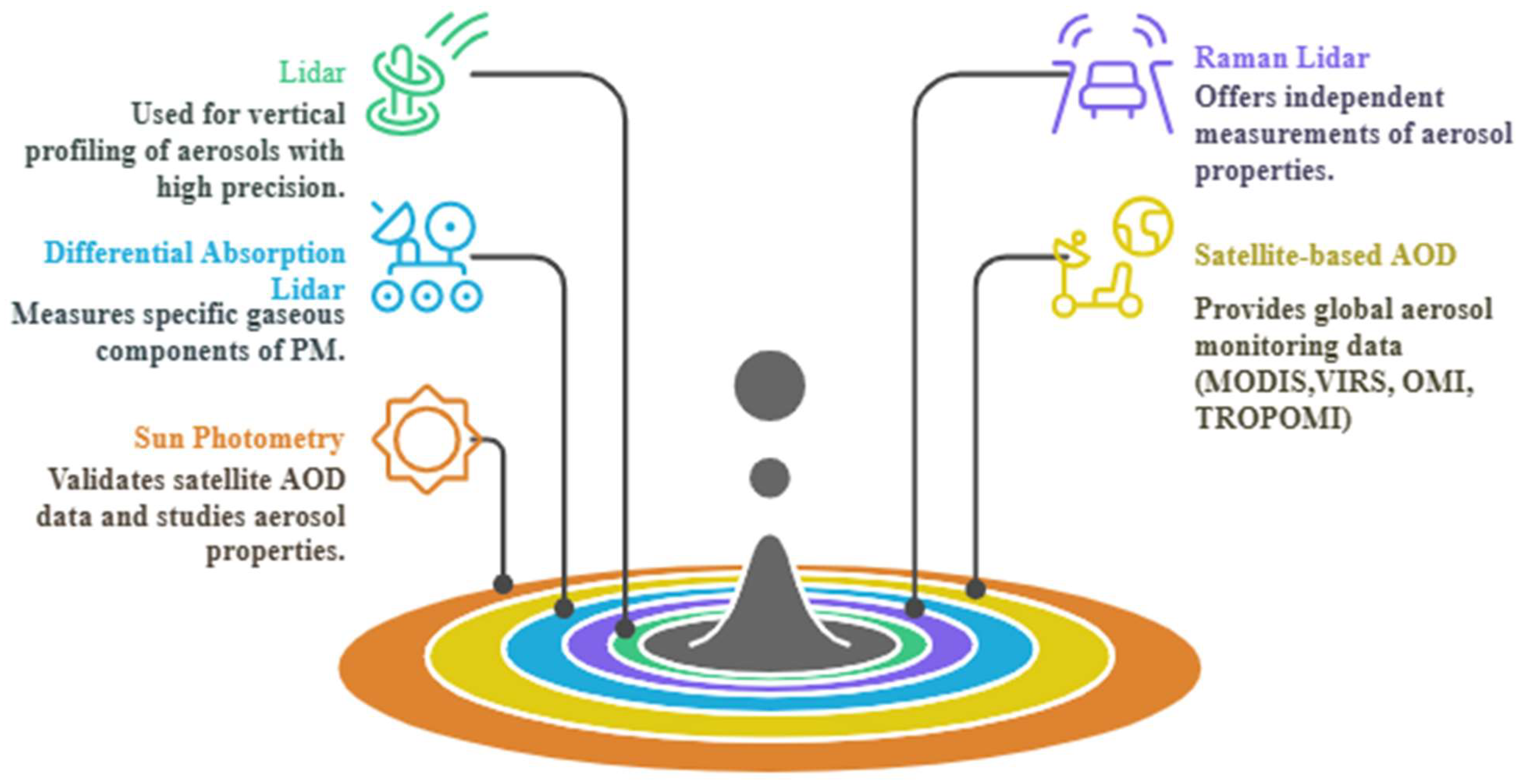
2.1.7. Remote Sensing Methods

Remote sensing methods have revolutionized the measurement of airborne PM, offering high spatial and temporal resolution data over large areas. These techniques include Lidar (Light Detection and Ranging), Raman Lidar, Differential Absorption Lidar (DIAL), satellite-based Aerosol Optical Depth (AOD) measurements, and Sun Photometry as shown in Figure 5.
Lidar technology has emerged as a powerful tool for vertical profiling of aerosols. Soupiona et al. (2020) utilized a multi-wavelength Raman lidar to characterize the vertical distribution of Saharan dust over Athens, Greece[67]. Their study demonstrated the capability of lidar systems to provide detailed information on aerosol layering and optical properties. Raman lidar, in particular, offers the advantage of independent measurements of aerosol extinction and backscatter coefficients, allowing for more accurate retrieval of aerosol properties.
Differential Absorption Lidar (DIAL) has been employed for measuring specific gaseous components of PM. Browell et al. (1998) demonstrated the use of airborne DIAL systems to simultaneously measure vertical distributions of water vapor and aerosols, showcasing the technique's potential for studying atmospheric composition and aerosol-water vapor interactions[68]. Their work highlighted the versatility of DIAL in providing high-resolution profiles of multiple atmospheric constituents. The satellite-based AOD measurements have become increasingly important for global aerosol monitoring. Lyapustin et al. (2018) introduced the MAIAC algorithm for MODIS AOD retrievals, which provides high-resolution (1 km) daily AOD data globally[69]. This advancement has significantly improved our ability to study aerosol distributions and trends over large areas. Wei et al. (2021) further demonstrated the application of satellite-derived AOD in estimating ground-level PM2.5 concentrations, highlighting the importance of these measurements for air quality studies[70].
Sun photometry remains a crucial ground-based technique for validating satellite AOD retrievals and studying aerosol properties. Giles et al. (2019) provided an overview of the AERONET Version 3 database, which includes improved automated cloud screening and quality control algorithms for sun photometer AOD measurements[71]. This update has significantly enhanced the accuracy and reliability of AERONET data, serving as a crucial ground truth for satellite and model validation. The integration of these remote sensing techniques offers unique advantages over traditional in-situ measurements. Benavent-Oltra et al. (2019) demonstrated the synergy between lidar and sun photometer measurements by using the GRASP (Generalized Retrieval of Aerosol and Surface Properties) algorithm to retrieve detailed aerosol optical and microphysical properties[72]. Their study, conducted during the SLOPE I and II campaigns in Granada, Spain, showcased how combining these remote sensing techniques can provide comprehensive information on aerosol characteristics, including vertical profiles of fine and coarse mode concentrations. Similarly, Siomos et al. (2020) used a combination of lidar and sun photometer measurements to study the impact of aerosols on solar radiation, showcasing the complementary nature of these techniques[73]. These remote sensing methods are particularly valuable for their ability to provide continuous, large-scale measurements that are not feasible with ground-based instruments alone. However, they also face challenges such as cloud interference in satellite retrievals and the need for complex retrieval algorithms to convert optical measurements into PM concentrations.
Despite their significant advantages, remote sensing methods for measuring airborne PM face several limitations and challenges. One major issue is the indirect nature of these measurements, which often require complex algorithms to convert optical properties to particle concentrations. As noted by Toth et al. (2014), the relationship between AOD and surface PM2.5 can vary significantly due to factors such as aerosol vertical distribution and relative humidity[74]. Satellite-based measurements are particularly affected by cloud cover and surface reflectance, which can lead to data gaps and retrieval errors. Li et al. (2016) highlighted the challenges in AOD retrievals over bright surfaces and in the presence of thin cirrus clouds[75]. Ground-based remote sensing techniques like lidar and sun photometry, while providing valuable vertical profile information, are limited in spatial coverage and can be affected by weather conditions. Wagner and Schäfer (2017) discussed the limitations of Raman lidar in measuring aerosols under high relative humidity conditions due to hygroscopic growth effects[76]. Additionally, the high cost and complexity of some remote sensing instruments, particularly advanced lidar systems, can limit their widespread deployment. These challenges underscore the need for integrated approaches that combine remote sensing with in-situ measurements and modeling to provide a more comprehensive understanding of airborne PM distributions and properties.

2.1.8. Emerging Low-Cost Sensor Technologies

While emerging low-cost sensor technologies are not traditionally considered part of the established methods for measuring airborne PM, however, they have gained significant attention in recent years due to their potential for widespread deployment and real-time monitoring. These technologies include various miniaturized light-scattering sensors, electrochemical sensors, and metal oxide semiconductor sensors.
Miniaturized light-scattering sensors have become popular for their ability to provide real-time measurements of PM concentrations. Bulot et al. (2019) evaluated the performance of low-cost PM sensors in a field study, demonstrating their potential for high-resolution spatial and temporal monitoring of air quality[77]. Their study showed that these sensors could capture pollution events and spatial variations that might be missed by traditional monitoring stations.
Electrochemical sensors have been applied to measure gaseous pollutants that often coexist with PM. Castell et al. (2017) assessed the performance of low-cost air quality sensors, including electrochemical sensors, in measuring NO2 and O3[78]. Their work highlighted the potential of these sensors for complementing existing air quality monitoring networks, especially in urban environments where pollution levels can vary significantly over short distances.
Metal oxide semiconductor sensors have shown promise in detecting various air pollutants. Karagulian et al. (2019) conducted a comprehensive review of low-cost sensors for air quality monitoring, including metal oxide sensors[79]. They noted that while these sensors face challenges in terms of accuracy and long-term stability, they offer unique advantages in terms of cost-effectiveness and the ability to provide high-resolution spatial data. The unique aspect of these emerging technologies lies in their potential for creating dense networks of air quality monitors. Morawska et al. (2018) discussed the paradigm shift in air pollution monitoring enabled by low-cost sensors, emphasizing their ability to provide unprecedented spatial and temporal resolution in air quality data[80]. However, it is important to note that these low-cost sensors are not without limitations. Rai et al. (2017) highlighted challenges such as cross-sensitivity to other pollutants, environmental factors affecting sensor performance, and the need for frequent calibration[81]. One major issue is the variability in sensor performance and data quality. Crilley et al. (2018) demonstrated that low-cost optical particle counters can be affected by relative humidity, potentially leading to overestimation of particle mass concentrations under high humidity conditions[39]. This highlights the need for careful calibration and correction algorithms to account for environmental factors. Another challenge is the long-term stability and drift of these sensors. Badura et al. (2018) observed significant sensor-to-sensor variability and temporal drift in low-cost PM sensors over a one-year deployment, emphasizing the need for regular recalibration and quality control measures[82]. Furthermore, the interpretation of data from dense networks of low-cost sensors presents its own challenges. Schneider et al. (2019) discussed the complexities of managing and interpreting large volumes of data from sensor networks, including issues of data quality assurance and the development of appropriate data analysis techniques[83]. These limitations underscore the importance of using low-cost sensors as complementary tools to established reference methods rather than as direct replacements. Addressing these challenges will be crucial for realizing the full potential of low-cost sensor technologies in air quality monitoring and management.

2.1.9. Hybrid and Multi-sensor Systems

Hybrid and multi-sensor systems, which combine multiple sensing techniques in a single instrument, have emerged as powerful tools for measuring airborne PM. These integrated approaches offer comprehensive characterization of aerosols by leveraging the strengths of different measurement principles.
Kosmopoulos et al. (2020) evaluated low-cost sensors for measuring PM2.5 and PM10, demonstrating that multi-sensor systems can provide reliable data when properly calibrated[84]. Their study highlighted the potential of these systems for expanding air quality monitoring networks cost-effectively. Alfano et al. (2020) reviewed various low-cost PM sensors, discussing how hybrid systems combining optical and electrical sensing methods can improve measurement accuracy across different particle size ranges[41]. They noted that such combinations could address limitations of single-method instruments, particularly in complex urban environments.
The integration of multiple sensing techniques can enhance the ability to distinguish between different types of PM. For instance, Bulot et al. (2019) deployed a network of low-cost sensors that combined optical particle counters with environmental sensors (temperature, humidity)[77]. This multi-parameter approach improved the accuracy of PM measurements and provided insights into the influence of meteorological conditions on PM concentrations. Advanced data fusion techniques have been crucial in maximizing the utility of multi-sensor systems. Concas et al. (2021) applied machine learning algorithms to combine data from low-cost PM sensors, meteorological instruments, and reference monitors[85]. Their approach significantly improved the accuracy of PM2.5 estimates compared to individual sensor readings.
The unique advantage of hybrid and multi-sensor systems lies in their ability to provide a more complete picture of aerosol properties and dynamics. Sousan et al. (2017) demonstrated that combining optical particle counting with electrical mobility analysis allowed for better characterization of particle morphology and density, which is crucial for understanding health impacts of different aerosol types[86]. These integrated approaches are particularly valuable in complex environments where single-method instruments may face limitations. Kuula et al. (2020) showed that a multi-sensor approach combining optical and electrical measurements was more robust in high-humidity conditions, where traditional optical sensors often struggle[35].
While hybrid systems offer numerous advantages, they also present challenges in terms of data integration and interpretation. Morawska et al. (2018) highlighted the importance of advanced calibration techniques when combining different sensor types, emphasizing the need for careful data processing to ensure accurate results[80]. The development of compact, field-deployable hybrid instruments has expanded the possibilities for widespread air quality monitoring. Jayaratne et al. (2018) described a portable system integrating particle counting, size distribution measurement, and gas sensors[87]. This multi-parameter approach provided comprehensive aerosol characterization in various urban and industrial settings. Looking forward, the integration of remote sensing techniques with in-situ measurements promises to further enhance our understanding of aerosol dynamics. Rybarczyk and Zalakeviciute (2018) reviewed various machine learning approaches for air quality modeling and forecasting, highlighting the potential of combining ground-based multi-sensor systems with advanced data analysis techniques to improve spatial coverage and prediction accuracy of PM concentrations[88].

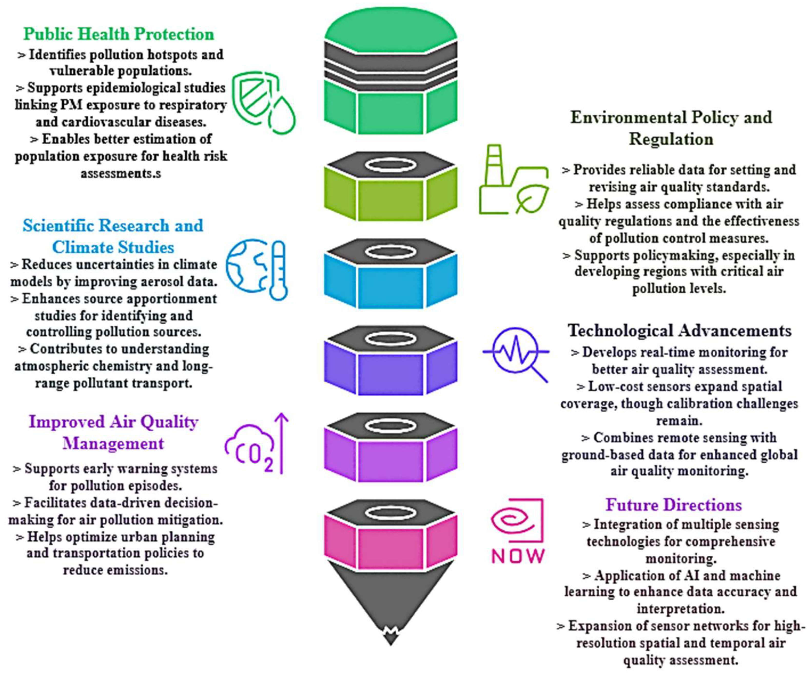
2.2. Significance of Accurate PM sensing for Air Quality Assessment

The significance of precise PM measurements extends across various domains, including public health, environmental policy, and scientific research, it is summed up in the Figure 6 . This section explores the multifaceted importance of accurate PM sensing and its implications for air quality assessment.
The primary driver for accurate PM sensing is its direct link to public health. Numerous epidemiological studies have established strong correlations between exposure to PM and adverse health outcomes. Pope and Dockery (2006) provided a comprehensive review of the health effects of fine particulate air pollution, highlighting associations with cardiovascular and respiratory diseases[89]. More recent studies, such as that by Chen et al. (2020), have further elucidated the relationship between long-term exposure to PM2.5 and mortality rates, emphasizing the need for accurate, long-term PM monitoring[90]. Accurate PM sensing allows for better estimation of population exposure, which is crucial for epidemiological studies and public health interventions. Brauer et al. (2012) demonstrated how improved PM2.5 estimates could enhance global exposure assessments, providing valuable data for burden of disease calculations[91]. Furthermore, precise PM measurements enable the identification of pollution hotspots and vulnerable populations, facilitating targeted interventions and resource allocation for public health initiatives.
In the realm of environmental policy and regulation, accurate PM sensing plays a vital role in shaping and enforcing air quality standards. Regulatory bodies rely on precise air quality data to set and revise ambient air quality standards. The work of Bachmann (2007) traced the historical development of PM standards in the United States, highlighting the critical role of scientific evidence derived from accurate measurements[92]. In Europe, Fuzzi et al. (2015) discussed how advancements in PM sensing technologies have influenced the evolution of air quality directives[66]. Moreover, accurate PM data is essential for assessing compliance with air quality standards and evaluating the effectiveness of pollution control measures. Pinder et al. (2019) demonstrated how improved PM2.5 measurements could enhance the assessment of Clean Air Act implementation in the United States[93]. In developing countries, where air pollution often reaches critical levels, accurate PM sensing is crucial for informing policy decisions and tracking progress in air quality improvement initiatives.
The significance of accurate PM sensing extends to scientific research and climate studies. PM plays a complex role in the Earth's radiative balance, and precise measurements are crucial for refining climate models. Boucher et al. (2013), in their contribution to the IPCC Fifth Assessment Report, emphasized the importance of accurate aerosol measurements for reducing uncertainties in climate projections[5]. Furthermore, accurate PM data is essential for source apportionment studies, which aim to identify and quantify the sources of particulate pollution. Belis et al. (2013) reviewed receptor models for source apportionment, underscoring the need for high-quality PM composition data[94]. Such studies are crucial for developing targeted emission control strategies and understanding the transport of pollutants across regions.
The quest for accurate PM sensing has driven significant technological advancements. Traditional gravimetric methods, while accurate, are labor-intensive and provide limited temporal resolution. Chow (1995) provided an early comprehensive review of measurement methods for PM[95]. Since then, the field has seen the development of various real-time monitoring techniques, including beta attenuation monitors, tapered element oscillating microbalances, and optical particle counters. More recently, low-cost sensor technologies have emerged as a promising tool for high-density PM monitoring networks. Snyder et al. (2013) discussed the potential of these sensors to complement existing regulatory monitoring networks[96]. However, ensuring the accuracy and reliability of these sensors remains a challenge. Morawska et al. (2018) highlighted the need for standardized evaluation protocols and calibration procedures for low-cost PM sensors[80].
Satellite-based remote sensing has also revolutionized PM monitoring, offering global coverage and high spatial resolution. van Donkelaar et al. (2016) demonstrated the use of satellite observations to estimate global PM2.5 concentrations, showcasing the potential of remote sensing for air quality assessment in areas lacking ground-based monitoring[97]. However, challenges remain in reconciling satellite-derived aerosol optical depth with ground-level PM concentrations, as discussed by Li et al. (2015)[98].
The future of accurate PM sensing lies in integrated approaches that combine multiple measurement techniques. Kulmala et al. (2021) proposed a global network of stations for atmospheric measurements, emphasizing the need for comprehensive, multi-instrument approaches to air quality monitoring[99]. Such integrated systems can provide a more complete picture of PM dynamics, from local to global scales. Machine learning and artificial intelligence are increasingly being applied to improve PM sensing accuracy and data interpretation. For instance, Di et al. (2019) demonstrated the use of neural networks to enhance PM2.5 estimates from low-cost sensors[100]. These advanced data processing techniques hold promise for extracting maximum value from diverse PM measurement sources.
The accurate PM sensing is hence fundamental to effective air quality assessment and management. Its significance spans public health protection, environmental policy formulation, and scientific research. As technology continues to advance, the integration of multiple sensing techniques, coupled with sophisticated data analysis methods, promises to further enhance our ability to monitor and understand PM pollution. This, in turn, will enable more effective strategies for improving air quality and mitigating the health and environmental impacts of PM pollution.
This section 2 has reviewed a range of traditional methods for measuring airborne PM, each with its own strengths and limitations. Gravimetric methods offer high accuracy for mass concentration measurements and allow for subsequent chemical analysis but are time-consuming and may be susceptible to artifacts. Continuous monitoring methods, such as BAM, TEOM, and QCM, provide real-time data but require careful calibration and may be affected by environmental factors. Optical methods are advantageous for real-time monitoring and size-resolved measurements, but their accuracy can be influenced by particle properties and environmental conditions. Electrical methods excel in measuring ultrafine particles and providing high-resolution size distributions but can be sensitive to particle charging effects and ambient conditions. Microscopy methods offer detailed insights into individual particle characteristics but are often limited by sample preparation requirements and the need for expert interpretation. Chemical analysis methods are essential for characterizing PM composition but face challenges related to sample preparation, the complexity of PM mixtures, and detection limits. Finally, remote sensing methods provide valuable spatial and temporal coverage but rely on complex algorithms and can be affected by factors like cloud cover. The choice of the most suitable method depends on the specific monitoring objectives, available resources, and desired level of accuracy and detail.

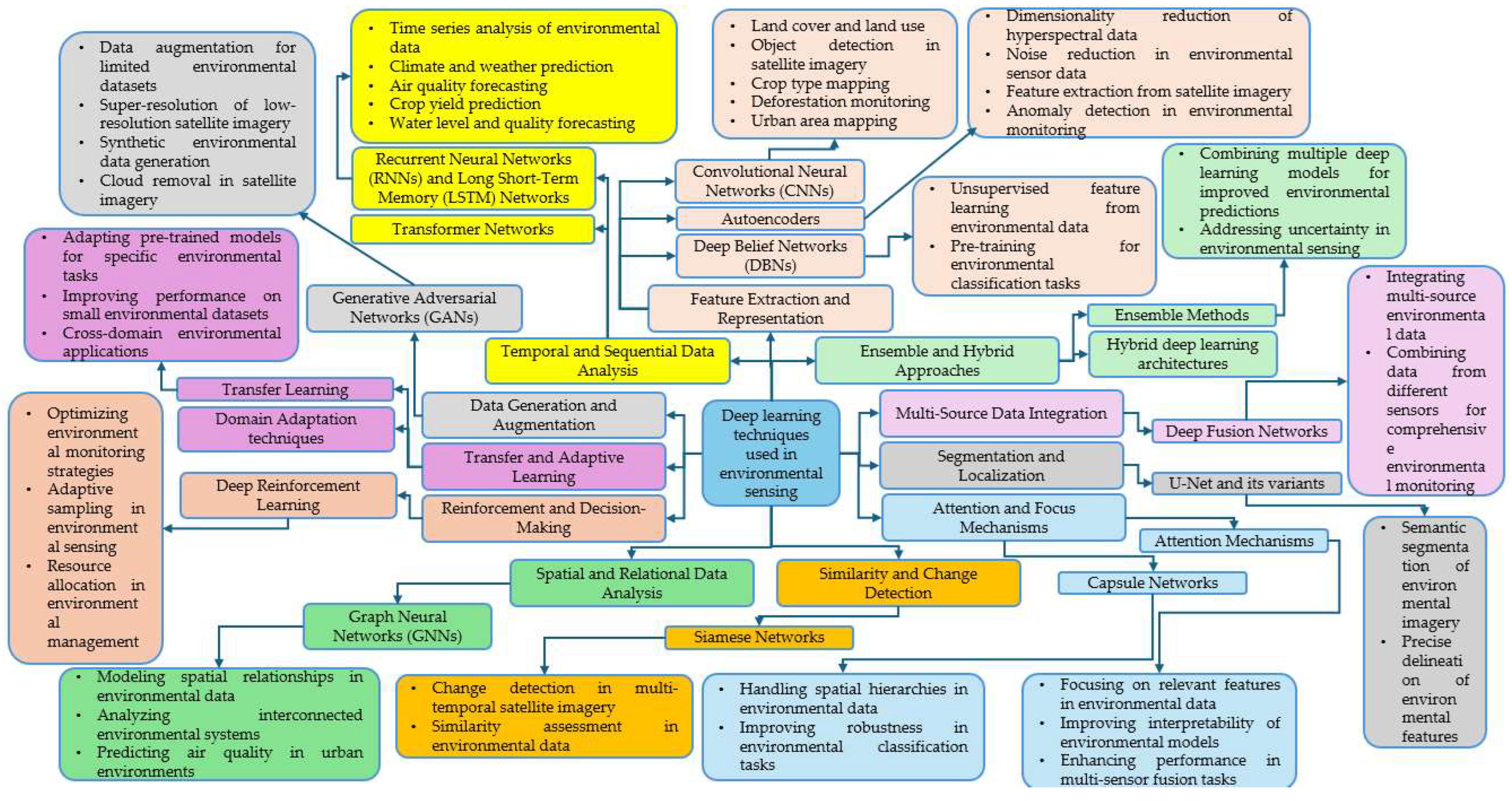
3. Deep Learning in Environmental Sensing:

The Figure 7 shows all the possible DL techniques and their roles in environmental sensing, organized by their use case is shown in the flow chart below. DL has emerged as a powerful tool in environmental sensing, revolutionizing the way we collect, process, and interpret environmental data. This section explores the application of DL techniques in environmental monitoring, focusing on their ability to extract meaningful features from complex environmental datasets. DL algorithms, particularly those based on ANN, have demonstrated remarkable success in tasks such as image classification, pattern recognition, and time series analysis, making them well-suited for addressing the challenges in the
The integration of DL with environmental sensing technologies has enabled more accurate and efficient monitoring of various environmental parameters, including air quality, water resources, land use changes, and climate patterns. These advanced techniques have the potential to overcome limitations of traditional methods, such as the ability to handle large volumes of heterogeneous data, extract complex features, and adapt to changing environmental conditions[102]. As this research delves into the specific DL architectures and their applications in environmental sensing, it will explore how these techniques are transforming our understanding of the environment and contributing to more effective environmental management strategies. The subsequent subsections are organised to show how DL can be used in various aspects of environmental sensing.

3.1. Data Processing and Feature Extraction

In the realm of environmental sensing, particularly for airborne PM, DL techniques have revolutionized data processing and feature extraction. This section explores the application of Convolutional Neural Networks (CNNs), Autoencoders, Deep Belief Networks (DBNs), and U-Net variants in environmental monitoring.
Table 1. Key applications of Deep Learning (DL) techniques in environmental sensing.
Technique Application Key Parameters Results Reference
DBN Estimating regional ground-level PM2.5 directly from satellite TOA reflectance Satellite top-of-atmosphere (TOA) reflectance The TOA-reflectance-derived PM2.5 has a finer resolution and a larger spatial coverage than the AOD-derived PM2.5. The deep learning-based model achieved state-of-the-art performance in estimating ground PM2.5 over the Wuhan Urban Agglomeration. [103]
GC-LSTM, LSTM Hourly PM2.5 concentration forecasting Historical air quality variables, meteorological factors, spatial terms, and temporal attributes The R2 value for 72-hour predictions using GC-LSTM was 0.72, compared to 0.13 using MLR. The GC-LSTM model outperformed other models, highlighting the importance of considering spatial and temporal dependency in forecasting PM2.5 concentrations. It also performed well in predicting over-standard PM2.5 concentrations. [104]
CNN Multi-hour and multi-site air quality index forecasting in Beijing Hourly measurements of six air pollutants (SO2, NO2, CO, O3, PM10, and PM2.5) and seven meteorological parameters (temperature, pressure, dew point, wind speed, wind direction, precipitation, and relative humidity) from 12 monitoring stations in Beijing. For overall forecasting, the CNN-LSTM model obtained an RMSE of 35.57 and an IA of 0.95, ranking as the best model. For spatial clustering-based forecasting, the CNN generally performed better than the other three models in terms of RMSE. [105]
Convolutional Denoising Autoencoder Imputation of missing values in air quality data Hourly measurements of different pollutants from multiple monitoring stations. The study considered 8 hours of data as input (temporal characteristic) from the target station and three neighboring stations (spatial characteristic), resulting in an input size of 8 x 4. The model achieved satisfying imputation results with R2 ≥ 0.6, even when data in the target station was entirely missing. Imputation performance decreased when correlations among stations were weak. The proposed model improved the average rate of improvement on RMSE (RIR) up to 65% compared to univariate imputation techniques and between 20% and 40% compared to multivariate techniques. [106]
Deep Recurrent Neural Network (DRNN) Predicting PM2.5 concentration levels in Japan Hourly measurements of PM2.5 concentrations, wind speed, wind direction, temperature, illuminance, humidity, and rain. The model used data from the target city and the three closest capital cities, considering 48 hours of past values as input. The DRNN model with dynamic pre-training (DynPT) outperformed a canonical autoencoder (CanAE) and a denoising autoencoder (DenAE) in terms of RMSE. It also achieved better performance than the existing PM2.5 prediction system VENUS, with an F-measure of 0.615 compared to 0.567 for VENUS. Using elastic net for sensor selection, the model could filter out unnecessary sensors (on average 2.1 sensors per city) without compromising prediction accuracy. [107]
CNNs with transfer learning, data augmentation, and CGANs. Air pollution prediction based on images from stationary cameras Images from a stationary camera, weather data (weather description, precipitation, humidity, visibility). The study considered images labeled based on PM2.5 sensor data according to six AQI categories and a binary classification (polluted vs. non-polluted). The custom pre-trained inception model, with CGAN data augmentation, obtained the best performance, achieving an accuracy of 0.896 on the training set and 0.763 on the testing set for binary classification. [108]
Conditional U-Net Emulating CMAQ simulations for PM2.5 concentration prediction and health impact assessment in South Korea Precursor emission activities (NO2, SO2, NH3, VOC, PM2.5) from 17 regions in South Korea and boundary conditions. The model achieved high accuracy in emulating CMAQ results, with a mean absolute error (MAE) of 0.221 µg/m3, a normalized MAE (NMAE) of 1.762%, and a coefficient of determination (R2) of 0.996. It also showed a significant reduction in computational time, requiring only 1 ms per scenario on a GPU compared to approximately 24 hours for a single CMAQ simulation. [109]
LSTM Air pollutant concentration prediction Hourly data of SO2, PM2.5, PM10, NO2, CO, O3, and AQI, along with nine meteorological factors, from 10 cities across China. For the prediction of PM2.5 concentration in the next hour, the LSTM model achieved an RMSE of 1.11 and an MAE of 0.66. [110]
DL techniques have significantly transformed environmental sensing, enabling more accurate, efficient, and scalable analysis of complex environmental data. Convolutional Neural Networks (CNNs) have proven particularly effective in handling spatial data from remote sensing imagery. Their ability to automatically learn hierarchical features from raw data has been demonstrated in various applications, such as land use classification and PM2.5 estimation from satellite imagery [111]. CNNs excel at extracting spatial features from satellite imagery and other geospatial data, making them effective for tasks like object detection in remote sensing images and estimating environmental parameters from visual data.
Autoencoders have found applications in dimensionality reduction and feature extraction from complex environmental datasets. These unsupervised learning models are particularly useful for handling high-dimensional data such as hyperspectral imagery. Riese and Keller (2019) showcased their potential in hyperspectral image classification for environmental monitoring applications [112]. Autoencoders help in capturing the most salient features of environmental data, which can be useful for tasks such as data compression, noise reduction, and anomaly detection.
Deep Belief Networks (DBNs) have shown promise in analyzing complex patterns in time-series data within environmental sensing. Ong et al. (2016) utilized DBNs for air quality prediction, achieving significant improvements over traditional methods [107]. DBNs are particularly useful for tasks that require understanding underlying structures in data, such as climate pattern analysis. Their layer-wise training process allows them to learn increasingly abstract representations of the input data, which can be beneficial for capturing long-term dependencies in environmental time series.
U-Net and its variants have demonstrated remarkable performance in image segmentation tasks crucial for environmental monitoring. Originally developed for biomedical image segmentation, U-Net has been successfully adapted for various environmental applications. Wieland et al. (2019) demonstrated the effectiveness of U-Net in cloud detection from satellite imagery [113]. Wei et al. (2020) adapted U-Net for building footprint extraction from high-resolution aerial imagery, showcasing its versatility in environmental remote sensing tasks [114]. The architecture's ability to capture both fine-grained details and broader contextual information makes it particularly suited for segmentation tasks in satellite and aerial imagery. These DL techniques have collectively improved our ability to extract meaningful information from large-scale satellite imagery, predict environmental parameters with higher accuracy, and detect subtle patterns in environmental data that might be missed by traditional methods.

3.2. Temporal and Sequential Analysis

Temporal and sequential analysis techniques have become increasingly important in environmental sensing, particularly for analyzing time-series data related to airborne PM and other environmental parameters. RNNs, Long Short-Term Memory (LSTM) networks, and Transformer networks have shown significant promise in capturing temporal dependencies and long-range interactions in environmental data.
Table 2. Key applications of Temporal and Sequential Analysis in environmental sensing.
Technique Application Key Parameters Results Reference
Self-tuning Spatio-temporal Neural Network (ST2NN) Air Quality Index (AQI) prediction Hourly concentration data of six major air pollutants and meteorological data collected at 12 monitoring stations in Beijing, China from March 1, 2013 to February 28, 2017. Across all four evaluation indexes, ST2NN outperformed the comparative models, improving prediction accuracy by 0.51%-10.18% (measured using R2). ST2NN achieved an R2 of 0.985, MSE of 2.357, RMSE of 1.467, and MAE of 1.132. [115]
Gated Recurrent Unit (GRU) Hourly PM2.5 concentration prediction in Shenyang, China. Hourly data of PM2.5, CO, NO, NO2, NOx, SO2, O3, PM10, factory emissions (particles, SO2, NOx, benchmark gas flow), meteorological data (atmospheric pressure, temperature, humidity, wind direction, wind speed), and temporal dummy variables (monthly, daily, hourly) from 11 monitoring sites and 187 plants in Shenyang, China. Data covers the winter seasons from 2015 to 2017. The model incorporated spatial information through convolutional processing of nearby pollutant measurements and factory emissions. The GRU-based model with convolutional processing achieved the best performance compared to baseline models (MLR, RF, SVM, ANN, traditional RNN, LSTM), with an MAE of 4.6147, MSE of 15.7878, and MAPE of 6.29%. The inclusion of both air quality and emission convolutional variables significantly improved the model's accuracy. Optimal performance was observed when using a dynamic time panel length (T) of 3, indicating the importance of considering historical data from the previous three hours for prediction. [116]
Graph Long Short-Term Memory with Multi-Head Attention (GLSTMMA) Hourly air pollutant concentration prediction. Hourly data of PM2.5, PM10, NO2, O3, SO2, CO, and AQI, along with seven meteorological factors and 12 categories of Point of Interest (POI) data, from 8 state-controlled stations in Qinghai Province, China from 2019 to 2021. The GLSTMMA model outperformed baseline models (Static, HA, VAR, LSTM, GRU, CNN-LSTM) across various prediction horizons (3, 6, 12, and 24 hours). For instance, for PM2.5 prediction at a 3-hour horizon, GLSTMMA achieved an MAE of 4.48, RMSE of 7.51, and MAPE of 34.44%. The model effectively leveraged spatial correlations between monitoring stations and temporal dependencies within the time series data, leading to improved prediction accuracy. [117]
Hybrid CNN-LSTM Daily PM2.5 concentration prediction in Beijing, China. Hourly data of PM2.5 concentration, dew point, temperature, atmospheric pressure, combined wind direction, cumulated wind speed, and cumulated hours of snow and rain from the US Embassy in Beijing and the Beijing Capital International Airport. The data covers a period with a total of 43800 records. The model uses the previous 7 days of data to predict the PM2.5 concentration of the next day. The multivariate CNN-LSTM model achieved the best performance compared to univariate LSTM, multivariate LSTM, and univariate CNN-LSTM models. It had an MAE of 13.9697 and RMSE of 17.9306. The model also had a shorter training time of 50-60 seconds per epoch, compared to 90-100 seconds for the other models. [118]
LSTM-Attention, n-step Attention-based Air Quality Predictor (n-step AAQP) Hourly PM2.5 concentration prediction in Beijing, China. Hourly data of SO2, CO, NO2, O3, PM2.5, PM10, precipitation, humidity, temperature, wind force, and wind direction. Data from April 2017 to February 2018 was used for training, and data from March 1 to March 7, 2018 was used for testing. The model uses the previous 24 hours of air quality and weather data to predict the PM2.5 concentration for the subsequent 24 hours. The 12-step AAQP (LSTM) achieved the best performance at the Olympic Center station with an MAE of 14.96 and R2 of 0.85. The 12-step AAQP (GRU) performed best at the Dongsi station with an MAE of 26.49 and R2 of 0.63. The n-step AAQP outperformed other models, including ANN, SVM, GRU, LSTM, seq2seq, seq2seq-mean, and seq2seq-attention. The study also found that using a fully connected encoder with position embedding significantly reduced training time while maintaining accuracy. [119]
VMD–GAT–BiLSTM Hourly PM2.5 concentration prediction in Beijing, China Hourly air quality data from 30 monitoring stations in Beijing, China, from January 1, 2017 to December 31, 2020. The data included PM2.5, PM10, CO, O3, and NO2, as well as meteorological factors (temperature, dew point, air pressure, precipitation, wind speed) and timestamps. The VMD module decomposed the data into 6 sub-sequences, and the GAT module used 2 graph attention layers. The VMD-GAT-BiLSTM model outperformed baseline models, including GRU, BiLSTM, CNN-LSTM, Transformer, (Graph Convolutional Networks) GCN-LSTM, and STGCN, on both short-term (1 to 24 hours) and long-term (up to 48 hours) predictions. The study also found that the VMD module significantly improved performance compared to using EMD or no decomposition. [120]
RNNs have been applied to various environmental sensing tasks due to their ability to process sequential data. These networks maintain an internal state that can capture information from previous time steps, making them suitable for time-series analysis. Recent advancements in RNN architectures have improved their ability to handle long-term dependencies, as demonstrated by Bianchi et al. (2021) in their work on air quality forecasting[121]. LSTM networks, a specialized form of RNNs, have gained widespread adoption in environmental sensing applications. Their unique architecture, featuring memory cells and gating mechanisms, allows for better preservation of long-term information. Zhao et al. (2019) showcased the effectiveness of LSTMs in air quality prediction, achieving significant improvements over traditional time-series models[122].
More recently, Transformer networks have gained traction in environmental sensing due to their ability to capture long-range dependencies without the need for recurrence. Originally proposed for natural language processing tasks, Transformers use self-attention mechanisms to weigh the importance of different input elements. Sonderby et al. (2020) demonstrated the superiority of Transformer models in precipitation nowcasting, outperforming conventional CNN-LSTM approaches[123].
RNNs and LSTMs have demonstrated effectiveness in various environmental sensing tasks. For instance, Wen et al. (2019) applied RNNs to PM2.5 concentration prediction, achieving a 21% RMSE reduction compared to ARIMA models[124]. Zhao et al. (2019) showcased LSTM networks' capability in air quality forecasting, with a 15% accuracy improvement over traditional methods[122]. More recently, Transformer networks have gained traction due to their ability to capture long-range dependencies without recurrence. Sonderby et al. (2020) demonstrated the superiority of Transformer models in precipitation nowcasting, outperforming conventional CNN-LSTM approaches[123]. Hybrid approaches, combining different techniques, have emerged as a promising direction. Li et al. (2020) demonstrated that integrating RNN and LSTM layers can leverage the strengths of both architectures, leading to improved urban air quality predictions[118]. Similarly, recent studies have incorporated attention mechanisms into LSTM networks, enhancing the model's ability to focus on relevant temporal patterns in air pollutant concentration data.

3.3. Advanced Learning Paradigms

These techniques offer innovative solutions to challenges such as limited labeled data, domain shifts, and complex decision-making processes in environmental monitoring. Transfer learning has gained significant traction in environmental sensing applications, allowing models trained on large datasets to be fine-tuned for specific tasks with limited data. Transfer learning has shown significant promise in land cover classification tasks using remote sensing data. For instance, Peng et al. (2019) demonstrated the effectiveness of transfer learning in improving the accuracy of land cover change detection using high-resolution satellite imagery[125]. Their approach, which utilized a modified UNet++ architecture, achieved superior performance compared to traditional methods.
Domain adaptation techniques address the challenge of distributional shifts between source and target domains, a common issue in environmental monitoring where sensor data may vary across different locations or time periods. These methods have been successfully applied to adapt models trained on one set of environmental conditions to perform well in different settings. For instance, Qi et al. (2019) developed a hybrid model combining graph convolutional neural networks and long short-term memory networks to improve PM2.5 forecasting across different urban environments[104].
Deep reinforcement learning (DRL) has shown promise in optimizing sensor placement and data collection strategies for environmental monitoring. By formulating the sensing process as a decision-making problem, DRL algorithms can learn optimal policies for sensor deployment and data acquisition. While not specifically focused on sensor placement, Tao et al. (2019) demonstrated the effectiveness of DL techniques, combining 1D convolutional neural networks and bidirectional gated recurrent units (GRU), for air pollution forecasting[126]. Their approach showcases how advanced DL methods can capture complex temporal patterns in air quality data, which is relevant to optimizing environmental sensing strategies.
Generative Adversarial Networks (GANs) have found applications in data augmentation and synthetic data generation for environmental sensing tasks. This is particularly valuable in scenarios where real-world data collection is challenging or expensive. Jacob et al. (2022) employed GANs to generate synthetic airborne PM images, enhancing the training dataset for detection algorithms[127]. Table 3 summarizes the key research applications of these advanced learning paradigms in environmental sensing:
These advanced learning paradigms have significantly enhanced the capabilities of DL models in environmental sensing applications. Transfer learning and domain adaptation techniques have proven particularly valuable in scenarios with limited labeled data or when adapting models to new environments. For instance, Njaime et al. (2024) demonstrated how transfer learning could improve the performance of DL models for air quality prediction in smart cities, addressing the challenge of data scarcity in new locations[134]. Deep reinforcement learning has opened new avenues for optimizing sensing strategies and resource allocation in environmental monitoring networks. The work by Wei et al. (2017) showcases how DRL can be used to develop adaptive control strategies for HVAC systems, significantly reducing energy consumption while maintaining occupant comfort in buildings[135].
GANs have not only contributed to data augmentation but also shown promise in anomaly detection for environmental data. Zeng et al. (2020) utilized GANs to generate synthetic images for data augmentation in citrus disease detection, improving the performance of DL models in agricultural monitoring applications[133]. The integration of these advanced learning paradigms with traditional sensing technologies has led to more robust and efficient environmental monitoring systems. For example, Sonawani and Patil (2024) proposed an IoT-based air quality measurement and prediction system that uses transfer learning to improve performance in new environments with insufficient data[136].

3.4. Spatial and Relational Analysis

Spatial and relational analysis techniques have significantly enhanced DL applications in environmental sensing (summarized in Table 4). These approaches enable models to capture complex spatial dependencies and relationships within environmental data, leading to improved performance in tasks such as air quality prediction, land use classification, and pollution source identification.
Graph Neural Networks (GNNs) have shown particular promise in modeling the interconnected nature of environmental systems. By representing data as nodes and edges in a graph structure, GNNs can effectively capture spatial correlations and propagate information across different locations. For instance, Qi et al. (2020) applied a Graph Convolutional Network to model the spatial dependencies between air quality monitoring stations, achieving superior performance in PM2.5 concentration prediction compared to traditional methods[104].
Attention mechanisms have been widely adopted in environmental sensing tasks, allowing models to focus on the most relevant features or spatial regions. This approach has proven especially effective in handling heterogeneous data sources and capturing long-range dependencies. Cheng et al. (2020) incorporated a spatial attention mechanism into their DL model for air quality forecasting, enabling the network to adaptively weight the importance of different monitoring stations based on their relevance to the target location[137].
While less extensively explored in environmental sensing compared to GNNs and attention mechanisms, Capsule Networks offer potential advantages in capturing hierarchical spatial relationships and maintaining equivariance. These properties could be particularly valuable in applications such as remote sensing image analysis for environmental monitoring. Zhang et al. (2018) applied a CapsNet architecture to hyperspectral image classification, achieving high accuracy in distinguishing various land cover types[138].

3.5. Ensemble and Multi-Source Integration

Ensemble and multi-source integration techniques have emerged as powerful approaches in DL for environmental sensing, enabling more robust and accurate predictions by combining multiple models or data sources. These methods leverage the strengths of different architectures and input modalities to overcome limitations of individual models and capture complex environmental patterns.
Ensemble methods in environmental sensing often combine predictions from multiple DL models to improve overall performance. For instance, Yi et al. (2018) developed a deep distributed fusion network for air quality prediction, which integrates data from various sources such as air quality data, meteorological data, and weather forecasts[145]. This approach demonstrated significant improvements in prediction accuracy by leveraging the strengths of different data types.
Hybrid DL architectures integrate different neural network types within a single model. For example, a hybrid CNN-LSTM architecture can be used for PM2.5 concentration prediction, where CNNs extract spatial features from air quality and meteorological data, while LSTMs capture temporal dependencies. This hybrid approach outperforms individual CNN and LSTM models in forecasting accuracy. Deep fusion networks have shown promise in integrating multi-source environmental data. Wen et al. (2019) developed a spatiotemporal convolutional long short-term neural network for air pollution prediction, which effectively integrates spatial and temporal data to enhance prediction accuracy[124]. This method allows for more comprehensive assessments by fusing heterogeneous data inputs.
Siamese networks have been applied for tasks like identifying corresponding patches in multi-modal satellite imagery. Hughes et al. (2018) utilized a Pseudo-Siamese CNN architecture to match SAR and optical image patches, demonstrating the potential of this approach for multi-sensor environmental monitoring applications[146].
Table 5. Applications of Ensemble and Multi-Source Integration Techniques in Environmental Sensing.
Technique Application Architecture Key Parameters Performance Metrics Reference
Hybrid PM2.5 forecasting CNN-LSTM 3 CNN layers, 2 LSTM layers RMSE: 7.5 μg/m³, R²: 0.92 [147]
Hybrid PM2.5 prediction OR-ELM-AR model Online recurrent extreme learning machine, autoregressive model R²: 0.85, RMSE: 12.3 μg/m³ [148]
DL PM2.5 prediction CNN-LSTM-MLP hybrid model Weighted LSTM extended model (WLSTME) RMSE: 8.216 μg/m³, R²: 0.91 [149]
Hybrid PM2.5 prediction Graph Convolutional Network with LSTM 3 graph conv layers, 1 LSTM layer, 64 hidden units MAE: 8.7 μg/m³, R²: 0.86 [104]
Hybrid Ensemble PM2.5 and PM10 forecasting CNN with spatial-temporal attention and residual learning Multi-step ahead forecasting system R² > 0.90 for both PM2.5 and PM10 [150]
Deep Fusion Air quality prediction Deep distributed fusion network Spatial transformation component, neural distributed architecture Improved accuracy over 10 baseline methods [145]
Hybrid Air pollution prediction Spatiotemporal convolutional LSTM 2 LSTM layers, 128 hidden units, spatiotemporal conv layers MAPE: 11.93%, R²: 0.86 [124]
Siamese Network Land cover change detection Siamese CNN Shared weights across twin networks Overall Accuracy: 92% [146]
These ensemble and multi-source integration techniques have demonstrated significant improvements in environmental sensing tasks by leveraging complementary strengths of different models and data sources. As environmental monitoring systems continue to evolve, incorporating diverse data streams and sensor types, these approaches are likely to play an increasingly important role in extracting meaningful insights and improving prediction accuracy.
Deep learning (DL) significantly enhances the accuracy of airborne PM sensing compared to traditional methods in several key ways such as, Feature Extraction: DL algorithms, particularly Convolutional Neural Networks (CNNs), excel at automatically extracting complex features and patterns from raw data, such as images and time series, that traditional methods might overlook. This automated feature extraction reduces the reliance on manual feature engineering, which can be subjective and time-consuming.; Nonlinear Relationships: DL models can effectively capture nonlinear relationships between PM concentrations and various influencing factors, including meteorological conditions, traffic patterns, and land use. Traditional methods often struggle to model these complex, nonlinear dependencies, leading to lower accuracy.; Spatial and Temporal Analysis: DL techniques, like GCNs and RNNs, are adept at capturing spatial and temporal dependencies within PM data. This capability allows DL models to account for the influence of neighboring areas and historical trends on PM concentrations, leading to more accurate predictions.; Data Fusion: DL facilitates the integration of data from multiple sources, such as satellite imagery, ground-based sensors, and meteorological data. By fusing these diverse datasets, DL models can provide a more comprehensive and accurate representation of PM dynamics compared to traditional methods that typically rely on single-source data.; Adaptive Learning: DL models can continuously adapt and improve their performance as they are exposed to more data. This adaptive learning capability allows DL models to refine their understanding of PM dynamics over time, leading to higher accuracy and better generalization to new environments or conditions.
This section has explored a variety of deep learning techniques for environmental sensing, each offering unique advantages and facing certain limitations. CNNs excel at extracting spatial features from images and have proven successful in tasks like air quality estimation from visual data. However, they may require large datasets for training and can be computationally intensive. Autoencoders are effective for dimensionality reduction and anomaly detection but may struggle with capturing complex temporal patterns. RNNs, particularly LSTMs, are well-suited for handling time series data and have been successfully applied to air quality forecasting. However, they can be prone to vanishing gradients and may require careful tuning. Advanced learning paradigms, such as transfer learning, reinforcement learning, and GANs, offer innovative solutions for addressing challenges like limited labeled data, complex decision-making, and synthetic data generation. Spatial and relational analysis techniques, including graph neural networks, attention mechanisms, and convolutional LSTMs, have enhanced the ability of deep learning models to capture complex spatial dependencies and relationships, leading to improved accuracy in tasks like PM2.5 prediction and land use classification. The choice of the most suitable deep learning technique depends on the specific environmental sensing task, the nature of the data, and the available computational resources.

4. Integration of DL with Airborne PM Sensing

The integration of DL with airborne PM (PM) sensing has led to significant advancements in environmental monitoring and air quality assessment, some of the studies are mentioned in the Table 6. Recent studies shown in the table below have explored novel approaches to enhance the accuracy and efficiency of PM sensing systems.
Yan et al. (2020) introduced EntityDenseNet, an interpretable DL model designed to retrieve ground-level PM2.5 concentrations from geostationary satellite data [151]. This model achieved impressive accuracy metrics, with hourly RMSE of 26.85 μg/m³, daily RMSE of 25.3 μg/m³, and monthly RMSE of 15.34 μg/m³. Notably, EntityDenseNet outperformed traditional machine learning methods such as BPNN, XGBoost, LightGBM, and Random Forest in both correlation (R²) and RMSE. The model's ability to automatically extract PM2.5 spatio-temporal characteristics allowed for insights into regional pollution influences and seasonal patterns.
In the realm of sensor network optimization, Lee et al. (2023) proposed an intelligent PM2.5 mass concentration analyzer that combines DL algorithms with an improved density measurement chip [159]. This approach aims to enhance the accuracy of airborne particle sensor networks, addressing the limitations of traditional optical particle counters in distinguishing between particles of different compositions but similar sizes. The study highlights the potential for integrating advanced hardware with DL techniques to improve PM2.5 monitoring accuracy.
A notable innovation in this field is the development of smartphone-based digital holographic microscopy (S-DHM) combined with DL for PM monitoring. Kim et al. (2021) introduced a novel technique using S-DHM and a DL network called Holo-SpeckleNet, which can estimate PM10 and PM2.5 concentrations from holographic speckle patterns with high throughput and accuracy [160]. This approach achieved relative errors of 11.23% ± 9.32% for PM10 and 5.81% ± 4.46% for PM2.5 concentrations, processing 100 holograms in just 1.57 seconds. Such mobile-optics integration represents a promising direction for portable PM monitoring, especially in hazardous environments. Additionally, Grant-Jacob and Mills (2022) reviewed various DL applications in airborne PM sensing, highlighting the potential of using complementary metal-oxide-semiconductor (CMOS) sensors or charged coupled device (CCD) detector arrays to capture more detailed scattering patterns from particles [127]. This 'lensless' sensing method, combined with neural networks, offers new possibilities for identifying different types of particulates based on their unique scattering signatures.
The use of DL models for air quality estimation using image data has got significant attention. Zhang et al. (2020) proposed a novel DL model called AQC-Net for estimating air quality levels from scene images [161]. The model incorporates a self-supervision module called Spatial and Context Attention (SCA) block, which enhances feature representation by capturing interdependence between channel maps. AQC-Net was trained and evaluated on a high-quality outdoor air quality dataset (NWNU-AQI) compiled by the authors. The model demonstrated superior performance in air quality classification compared to traditional methods like Support Vector Machine (SVM) and Deep Residual Network (ResNet). This approach offers a complementary method to traditional air quality monitoring stations, particularly useful for areas far from established monitoring sites. However, the authors note limitations such as the model's focus on daytime images and potential regional specificity, suggesting the need for local retraining when applied to different geographical areas. Li et al. (2018) presented a novel DL framework for satellite-based PM2.5 estimation[162]. Their approach demonstrated versatility in both AOD-based and reflectance-based PM2.5 estimation. For AOD-based estimation across China, the model achieved impressive performance with cross-validation R² and RMSE values of 0.88 and 13.03 μg/m³, respectively. The study also explored direct PM2.5 estimation from satellite top-of-atmosphere (TOA) reflectance data in the Wuhan Metropolitan Area, achieving cross-validation R² and RMSE values of 0.87 and 9.89 μg/m³. This reflectance-based approach eliminates the need for intermediate AOD retrieval, potentially simplifying the estimation process. The framework's ability to capture nonlinear relationships between PM2.5 and satellite observations, as well as its effectiveness in producing daily PM2.5 estimates with high spatial resolution, highlights the potential of DL in enhancing satellite-based air quality monitoring.
The integration of DL with airborne PM sensing has demonstrated significant potential in enhancing the accuracy, efficiency, and accessibility of air quality monitoring. From satellite-based estimations to smartphone-enabled portable devices, DL approaches have shown remarkable improvements over traditional methods. These advancements offer promising solutions for real-time, high-resolution PM monitoring, particularly in areas with limited access to conventional monitoring stations. Section 4 showcased the remarkable progress in integrating deep learning with airborne PM sensing technologies. The studies discussed exemplify how deep learning is enhancing various aspects of PM monitoring, from improving the accuracy of satellite-based PM2.5 estimations to enabling the development of portable, smartphone-based PM sensors. This integration is revolutionizing the field, offering promising solutions for real-time, high-resolution PM monitoring, especially in areas lacking traditional monitoring infrastructure.

5. Data Acquisition and use of synthetic data for Air Quality Monitoring

The effectiveness of DL models in airborne PM (PM) sensing heavily relies on the quality and quantity of available data. This section explores the challenges in data acquisition and preprocessing from airborne PM sensors, techniques for handling large and noisy datasets, and the importance of data quality in developing effective DL models for air quality monitoring.

5.1. Challenges in acquiring and pre-processing data from airborne PM sensors

Acquiring high-quality data from airborne PM sensors presents several challenges that researchers and practitioners must address to ensure the reliability and effectiveness of DL models in air quality monitoring.
Sensor Calibration and Drift: Low-cost PM sensors, while offering the advantage of widespread deployment, often require careful calibration to ensure accurate measurements. Zimmerman et al. (2018) demonstrated that machine learning techniques, particularly random forest models, can significantly improve the calibration of low-cost PM2.5 sensors [163]. Their study showed an increase in R² values from 0.24-0.62 for uncalibrated sensors to 0.68-0.76 when compared to reference instruments. However, sensor drift over time remains a challenge, necessitating regular recalibration or the development of adaptive calibration methods.
Environmental Variability : PM concentrations can vary significantly due to factors such as temperature, humidity, and wind patterns. A study by Li et al. (2017) explores the use of Long Short-Term Memory (LSTM) neural networks for air pollutant concentration predictions, including PM2.5, while considering meteorological conditions[164]. The authors demonstrate that their LSTM model outperforms traditional approaches in predicting air pollutant concentrations, highlighting the importance of incorporating meteorological data in DL models for air quality prediction.
Spatial and Temporal Resolution : Achieving high spatial and temporal resolution in PM data collection is crucial for accurate modeling but often challenging due to limitations in sensor deployment and data transmission. A study by Li et al. (2017) presents a geo -intelligent DL approach that fuses satellite and ground station observations to estimate ground-level PM2.5 concentrations [165]. The authors demonstrate that their method achieves high-resolution PM2.5 estimation by effectively integrating multiple data sources.
Data Gaps and Missing Values: Sensor malfunctions, power outages, or communication failures can lead to gaps in PM data collection. Handling these missing values is crucial for maintaining the continuity and reliability of air quality monitoring. Wei et al. (2021) made significant contributions by developing a method to reconstruct high-resolution PM2.5 data in China over an extended period [70]. Their study employed a space-time extremely randomized trees (STET) model, which combines satellite aerosol optical depth data with other relevant variables to estimate ground-level PM2.5 concentrations. This approach is particularly noteworthy for its ability to create consistent long-term records of PM2.5 concentrations, addressing a critical challenge in air quality monitoring. The STET model's capacity to handle spatiotemporal variations and incorporate multiple data sources makes it a valuable tool for filling data gaps and enhancing the overall quality of PM2.5 datasets. By reconstructing PM2.5 data at a 1-km resolution from 2000 to 2018, Wei et al. demonstrated the potential of machine learning techniques in overcoming limitations in historical air quality data, providing a more comprehensive understanding of long-term PM2.5 trends and spatial distributions. This work represents a significant step forward in the application of advanced data processing techniques to improve the consistency and reliability of air quality monitoring data.
Interference from Other Pollutants: A significant challenge in airborne PM sensing is the interference from other pollutants, which can affect the accuracy and reliability of measurements. Thompson (2016) highlights this issue in his review of crowd-sourced air quality studies and portable sensors [166]. The author notes that certain low-cost sensors, such as metal oxide semiconductor (M.O.S.) sensors, while sensitive, lack the necessary selectivity for accurate air quality monitoring. These sensors can experience significant drift during use and may be prone to erroneous measurements due to cross-sensitivity with other gases. For instance, some M.O.S. sensors designed for one pollutant may respond to other gases present in the air, leading to inaccurate readings. Thompson emphasizes that when developing air quality monitoring networks, it should not be assumed that sensors work flawlessly. Instead, care must be taken to calibrate sensors and verify their performance routinely. This underscores the need for developing more selective sensing technologies or implementing methods to compensate for cross-sensitivities in existing sensors. The author suggests that significant resources should be directed towards improving sensor technology, particularly in enhancing selectivity, to achieve the transformative potential of crowd-sourced air quality monitoring.
Data standardization and Integeration: Integrating data from multiple sensor types and manufacturers poses challenges in data standardization for large-scale air quality monitoring networks. Morawska et al. (2018) conducted a comprehensive review of low-cost sensing technologies for air quality monitoring and exposure assessment[80]. They highlighted that the application of these technologies has already changed the paradigm of air pollution monitoring. The authors noted that current low-cost sensing technologies are capable of supplementing routine ambient air monitoring networks and expanding conversations with communities, often beyond single authorities responsible for air quality management. However, they also identified areas for improvement, particularly in enhancing source compliance monitoring, which is crucial for developing countries. The review emphasized the need for further work on personal exposure monitoring, which is more demanding due to factors such as volunteer engagement and device limitations. The authors suggested that with significant expansion of monitoring networks and improved data interpretation for individuals, the need for personal sensors might decrease for outdoor air pollution assessment. However, personal monitoring would remain important for indoor exposure assessment and for pollutants like ultrafine particles, which are not currently measurable with low-cost technologies.
Privacy and Ethical Considerations: As air quality monitoring increasingly relies on mobile and personal sensors, privacy concerns arise regarding the collection and use of location-based data. Castell et al. (2017) discussed the ethical implications of citizen-based air quality monitoring in their comprehensive evaluation of low-cost sensor platforms[78]. While their study primarily focused on the technical aspects and data quality of these sensors, it also highlighted important considerations for citizen science applications. The authors noted that low-cost platforms, despite their limitations in accuracy for regulatory or health purposes, can provide relative and aggregated information about observed air quality. This capability opens up new opportunities for citizen engagement in environmental monitoring. However, the study emphasizes that data quality is a pertinent concern, especially in citizen science applications where non-experts are collecting and interpreting data. The authors suggest that while these sensors may not be suitable for high-accuracy applications like legislative compliance or scientific exposure estimates, they can be valuable for raising awareness and engaging communities in local air quality monitoring. This implies that guidelines for responsible data collection and usage should consider not only privacy aspects but also the appropriate use and interpretation of data from these low-cost sensors, ensuring that citizens are aware of both the capabilities and limitations of the technology they are using.

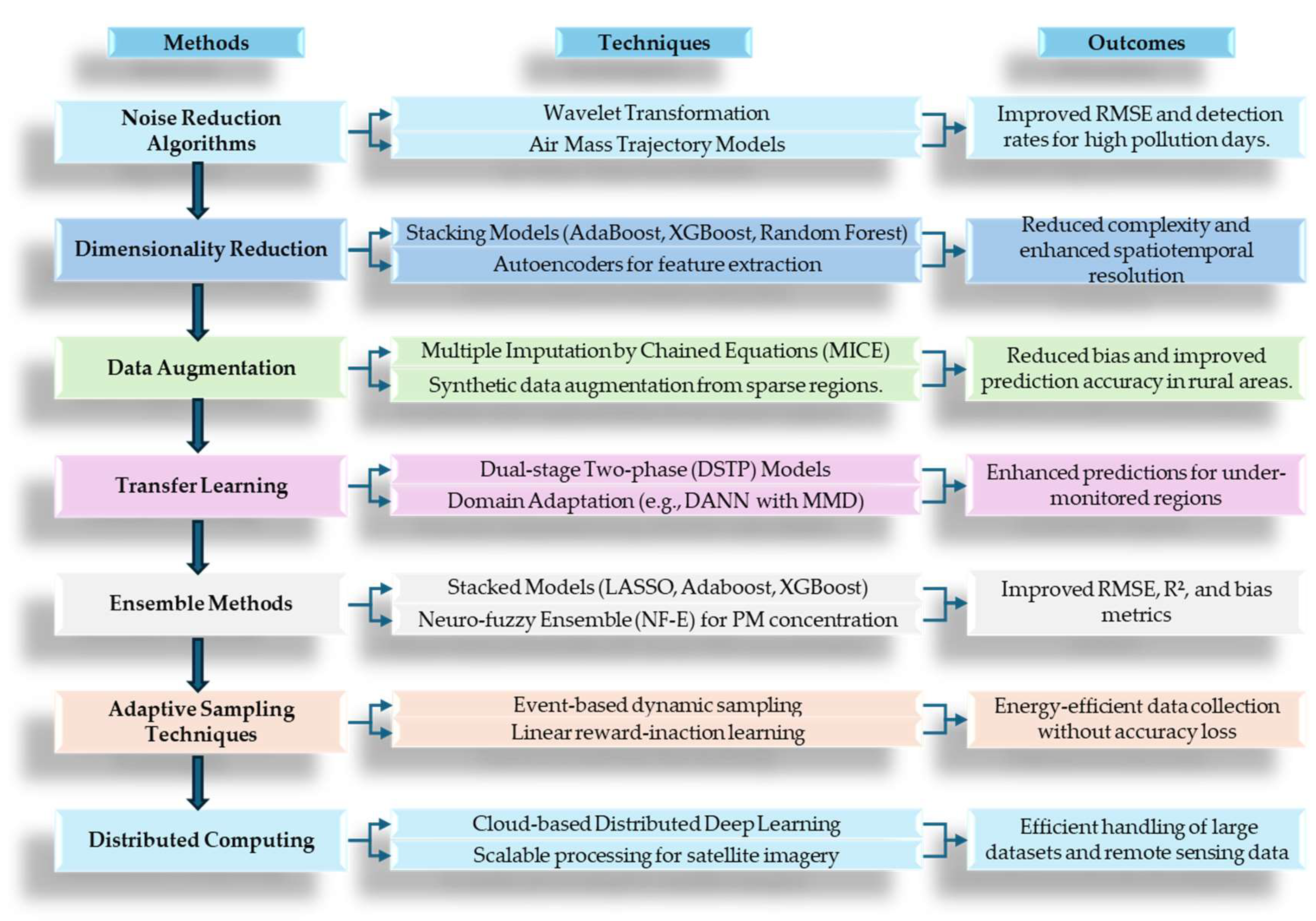
5.2. Techniques for handling noisy and large datasets

The nature of airborne PM sensing often results in large, noisy datasets that require sophisticated preprocessing and analysis techniques. Several approaches have been developed to address these challenges (the Figure 8 shows a flow chart techniques for handling noisy and large environmental datasets) :

5.2.1. Noise Reduction Algorithms

The study by Feng et al. (2015) demonstrates an effective approach to noise reduction in PM2.5 data through the application of wavelet transformation [167]. By decomposing the original PM2.5 time series into multiple sub-series with lower variability, the authors were able to separate high-frequency components (often associated with noise) from low-frequency components (representing underlying trends). This decomposition allowed for more effective handling of noisy components, thereby improving the overall data quality and prediction accuracy. The wavelet transformation, combined with an air mass trajectory-based geographic model and artificial neural networks, resulted in a significant reduction of the root mean squared error (RMSE) by up to 40% on average. Moreover, this approach enhanced the detection of high PM2.5 days, with the detection rate reaching 90% on average for a given alert threshold. By dividing the prediction problem into simpler tasks through wavelet decomposition, the authors were able to address the noise in the data more effectively, leading to improved forecasting accuracy and better anticipation of high pollution events. This hybrid model's success in noise reduction and improved PM2.5 forecasting demonstrates its potential for application in air quality forecasting systems in other regions.

5.2.2. Dimensionality Reduction

High-dimensional PM datasets c0an be challenging to process and may lead to overfitting in DL models. Chen et al. (2019) developed an innovative approach to estimate hourly PM2.5 concentrations using a stacking model that combines multiple machine learning algorithms [168]. The study utilized high-temporal resolution (1-hour) Aerosol Optical Depth (AOD) data from the geostationary satellite Himawari 8, along with meteorological and geographic data. The stacking model incorporated three submodels - AdaBoost, XGBoost, and Random Forest - which were then integrated using a multiple linear regression model. This approach effectively handled the high-dimensional dataset, which included satellite AOD, ground-based PM2.5 measurements, and various meteorological parameters. The stacking model outperformed individual models, achieving an average coefficient of determination (R²) of 0.85 and a root-mean-square error (RMSE) of 17.3 μg/m³. Notably, the model's performance peaked at 14:00 local time with an R² of 0.92 and RMSE of 12.9 μg/m³, demonstrating its effectiveness in processing and analyzing complex, multi-source PM2.5 data.
Wu et al. (2023) addressed the challenge of high-dimensional data in PM2.5 forecasting by employing an innovative hybrid DL model (AE-CNN-BP) [169]. The model utilizes an Autoencoder (AE) to effectively reduce the dimensionality of input data from 497 PM2.5 datasets (485 microsensors and 12 EPA stations) to a limited number of coded values. These coded values capture essential spatial characteristics of PM2.5 concentrations, significantly reducing data complexity while preserving crucial information. The AE's encoder compresses the high-dimensional input into a compact representation, while the decoder reconstructs the full dataset from these coded values. This dimensionality reduction approach not only helps in handling large, heterogeneous datasets but also addresses the issue of missing data from microsensors, enabling high-spatiotemporal-resolution forecasts of PM2.5 concentrations across a wide area.

5.2.3. Data Augmentation:

To address the issue of limited training data, especially in areas with sparse sensor coverage, data augmentation techniques have been employed. The study by Mi et al. (2024) directly addresses the issue of limited training data in areas with sparse sensor coverage through an innovative data augmentation technique. The authors propose a Multiple Imputation by Chained Equations Data Augmentation (MICE-DA) approach to remedy the dataset shift problem caused by the uneven distribution of air quality monitoring sites, which are predominantly located in urban areas. This method effectively augments the training dataset by accurately assimilating information from satellite-derived Aerosol Optical Depth (AOD) data, expanding spatial coverage and improving PM2.5 predictions in rural areas where ground-based sensors are scarce. The MICE-DA approach significantly reduced estimation bias, decreasing mean bias from -3.4 μg/m³ to -1.6 μg/m³, and enhanced the importance of AOD in predicting PM2.5 concentrations. By addressing the limitations of sparse sensor networks, particularly in rural regions, this data augmentation technique demonstrates a promising solution for improving the spatiotemporal resolution and accuracy of PM2.5 predictions in areas with limited ground-based monitoring.

5.2.4. Transfer Learning:

Transfer learning techniques have shown promise in adapting models trained on data-rich environments to areas with limited data availability, particularly for newly constructed monitoring sites. Ni et al. (2022) proposed an improved hybrid transfer learning model for PM2.5 concentration prediction[170]. Their approach combines a dual-stage two-phase (DSTP) model for spatial-temporal feature extraction with a domain adversarial neural network (DANN) for domain adaptation. The method uses maximum mean discrepancy (MMD) to select the most suitable source domain site for transfer learning. When applied to predict PM2.5 concentrations in Tianjin and Guangzhou using data from Beijing, their TL-DSTP-DANN model showed improvements of more than 8.5% in MAE, RMSE, and MAPE compared to other transfer learning prediction models. The study demonstrates that transfer learning can significantly enhance PM2.5 prediction performance in newly built monitoring stations with insufficient data, addressing the challenge of limited data availability in certain areas.

5.2.5. Ensemble Methods

Ensemble methods, which combine predictions from multiple models, have shown effectiveness in handling noisy PM data and improving forecasting accuracy. Zhai and Chen (2018) developed a stacked ensemble model for forecasting daily average PM2.5 concentrations in Beijing, China [171]. Their approach integrated multiple single models including LASSO, Adaboost, XGBoost, and a multi-layer perceptron optimized by a genetic algorithm (GA-MLP) in the level 0 space, which were then combined using support vector regression (SVR) in the level 1 space via stacked generalization. This ensemble model demonstrated superior performance compared to single nonlinear forecasting models, achieving a coefficient of determination (R²) of 0.90 and a root mean squared error (RMSE) of 23.69 μg/m³ when applied to new data. The ensemble approach showed improvements of 3.45% in R², 13.93% in bias, 18.98% in MAE, and 6.91% in RMSE compared to the best single model in the test set. This study highlights the potential of ensemble methods in enhancing PM2.5 forecasting accuracy and handling complex, noisy environmental data.
Umar et al. (2021) proposed a novel neuro-fuzzy ensemble (NF-E) model for predicting hourly PM2.5 and PM10 concentrations. Their approach combined four base models: Adaptive Neuro-Fuzzy Inference System (ANFIS), Artificial Neural Network (ANN), Support Vector Regression (SVR), and Multilinear Regression (MLR). The NF-E model used ANFIS as a nonlinear kernel to ensemble the outputs of these base models. This ensemble approach significantly outperformed individual base models and linear ensemble techniques, achieving Nash-Sutcliffe efficiency (NSE) values of 0.9594 and 0.9865 for PM2.5 and PM10 respectively in the testing stage. The NF-E model improved prediction efficiency by 4-22% for PM2.5 and 3-20% for PM10 compared to single models, demonstrating the potential of ensemble methods in enhancing PM concentration forecasting accuracy and handling complex, noisy environmental data.

5.2.6. Adaptive Sampling Techniques:

To manage large datasets efficiently and conserve energy in mobile sensing systems, adaptive sampling techniques have been explored. Rachuri (2013) introduced an adaptive sampling strategy that dynamically adjusts sensor sampling rates based on the user's context and observed events[172]. This approach uses linear reward-inaction learning based on learning automata theory to balance energy-accuracy tradeoffs. The technique increases sampling rates when interesting events are observed and decreases rates during periods of inactivity. Two adaptive schemes were evaluated: one using linear advance and exponential back-off, and another using exponential advance and linear back-off of sampling intervals. The study demonstrated that adaptive sampling could achieve significant energy savings compared to continuous sensing without compromising system accuracy. For example, the exponential back-off scheme showed more energy savings than the linear back-off scheme in purely local sensing scenarios. This adaptive approach allows mobile sensing applications to optimize data collection, potentially reducing data volume while maintaining the accuracy of PM monitoring systems.

5.2.7. Distributed Computing:

Processing large PM datasets often requires significant computational resources. Haut et al. (2021) provide a comprehensive review of distributed DL approaches for remote sensing data interpretation, which is applicable to PM monitoring using satellite imagery[173]. The authors highlight the potential of cloud computing systems for managing vast amounts of remotely sensed data, offering implementation simplicity, low cost, and high efficiency compared to other parallel and distributed architectures. They emphasize that technological advances in hardware and software have enabled the acquisition and processing of huge amounts of remotely sensed data with high spatial resolution and spectral dimensionality. The review suggests that cloud-based implementations of DL algorithms can effectively address the processing challenges involved in extracting information from large-scale remotely sensed images, including those used for PM monitoring. While specific performance metrics for PM2.5 forecasting are not provided, the authors indicate that cloud computing architectures can significantly improve processing capabilities for big data applications in remote sensing.

5.3. Importance of data quality for effective DL models

The quality of input data is paramount for the development of accurate and reliable DL models in airborne PM sensing. Several aspects underscore the importance of data quality (the Figure 9 shows the stages of data quality):

5.3.1. Model Performance

High-quality data and effective model architectures are crucial for accurate air quality estimation using DL approaches. Zhang et al. (2020) proposed a novel DL model called AQC-Net for estimating air quality levels from scene images[161]. The model incorporates a self-supervision module called Spatial and Context Attention (SCA) block, which enhances feature representation by capturing interdependence between channel maps. AQC-Net was trained and evaluated on a high-quality outdoor air quality dataset (NWNU-AQI) compiled by the authors. The model demonstrated superior performance in air quality classification compared to traditional methods like Support Vector Machine (SVM) and Deep Residual Network (ResNet). Specifically, AQC-Net achieved a classification accuracy of 74% on the test set, outperforming ResNet18 (70.1%) and SVM (60%). The study highlights the importance of both high-quality datasets and innovative model architectures in improving the accuracy of air quality estimation using DL techniques.

5.3.2. Generalizability

Generalizability in DL models for PM2.5 prediction and air quality estimation refers to a model's ability to perform well on new, unseen data or in different geographical locations and conditions than those it was trained on. This concept encompasses several key aspects: cross-regional performance, where a model trained on data from one region can make accurate predictions in other regions with potentially different environmental conditions; versatility in data types, demonstrating the ability to work effectively with various input data formats such as AOD-based and reflectance-based satellite data; consistent performance across time, maintaining accuracy across different temporal scales (hourly, daily, monthly) and seasons; and adaptability to varying pollution levels, ensuring reliable predictions for both low and high pollution scenarios. A truly generalizable model exhibits robustness across these dimensions, making it valuable for wide-scale application in air quality monitoring and forecasting. Wang et al. (2022) demonstrated this concept with their SpatioTemporal Enhanced Neural Network (STENN) model, which showed strong spatial generalization ability for PM2.5 estimation across mainland China[174]. Their model achieved an R² of 0.89 in cross-validation, indicating robust performance across different regions. The STENN model also demonstrated temporal transferability, successfully extrapolating to years without ground-based monitoring data. This approach, which integrated spatial signals into a recurrent neural network, effectively incorporated the impact of spatial heterogeneity and time dependence of PM2.5, resulting in high-quality, high-resolution (1 km) annual PM2.5 products for China from 2014 to 2020. The model's ability to maintain accuracy and stability across different regions and time periods, especially in high-value estimations and spatial continuity, exemplifies the importance of generalizability in PM2.5 prediction models.

5.3.3. Interpretability

Interpretability in DL models for PM2.5 prediction and air quality estimation is crucial for understanding and explaining how a model arrives at its predictions, building trust in its outputs, and extracting meaningful insights from the data. For these models, interpretability encompasses several key aspects: identifying the most significant input variables through feature importance analysis, revealing spatial-temporal patterns in the data, providing insights into the model's decision-making process across different layers, enabling error analysis to understand the model's performance under various conditions, and generating meaningful visualizations to explain the model's workings to non-technical stakeholders. High-quality, well-structured data plays a vital role in enhancing interpretability by allowing the model to learn more accurate and meaningful representations of PM2.5 dynamics. This improved interpretability enables researchers to extract more reliable insights about pollution patterns, sources, and trends, ultimately leading to better-informed decisions in air quality management and policy-making.
The study by Yan et al. (2021) directly addresses the concept of interpretability in DL models for PM2.5 prediction[175]. Their Spatial-Temporal Interpretable DL Model (SIDLM) demonstrates enhanced interpretability compared to traditional "black box" machine learning methods. The SIDLM's ability to automatically extract PM2.5 spatiotemporal characteristics allows for deeper insights into pollution patterns. For instance, the model revealed the strong influence of the Tongzhou district on PM2.5 levels in Beijing's main urban area and identified that summer months (June-August) contributed less to overall PM2.5 concentrations. The model's interpretability is further enhanced by its "wide" and "deep" components and their joint learning process. Unlike ensemble methods that combine separately trained models, SIDLM's joint training approach allows its components to inform each other during the training process, potentially leading to more coherent and interpretable results. This improved interpretability not only enhances the model's predictive accuracy but also provides valuable insights for understanding regional pollution influences and seasonal patterns, which is crucial for effective air quality management and policy-making.

5.3.4. Robustness to Outliers:

High-quality datasets with properly handled outliers contribute to more robust models. Outliers are data points that significantly differ from other observations in a dataset, potentially arising from measurement errors, rare events, or extreme conditions. Robust models should maintain their performance and reliability even in the presence of such anomalous data points. Effective outlier detection and handling techniques can improve model stability, especially when dealing with environmental data like PM2.5 and PM10 concentrations, which can be subject to sudden spikes due to various factors.
The study by Gregório et al. (2022) explored the effects of seasonal decomposition on model performance, finding that removing seasonality from the data could negatively impact accuracy by smoothing out critical trends associated with traffic patterns[176]. The study by Gregório et al. (2022) presents a robust machine learning algorithm designed for forecasting PM10 and PM2.5 concentrations. This algorithm employs a multiple-input multiple-output linear regression model, which offers a straightforward yet effective approach to air quality prediction.
In the study by Ma et al. (2022), robustness to outliers is addressed through careful data preprocessing and modeling techniques that enhance the overall quality of PM2.5 retrieval [177]. The authors standardized the input data and removed outliers to mitigate their impact on model performance. They employed a piecewise linear interpolation model to fill data gaps, ensuring a continuous dataset while preserving time series properties. Additionally, they utilized the min-max scaler method to normalize the raw data, which helps balance dimensions and can reduce the influence of extreme values. By comparing six different machine learning algorithms—MLR, kNN, SVR, RT, RF, and BPNN—the study indirectly assessed the robustness of these models against outliers through performance evaluations. The use of 10-fold cross-validation further ensured consistent model performance across different data subsets, enhancing robustness. Although the Random Forest model achieved the highest accuracy, all models demonstrated lower prediction accuracy in high-value areas, indicating potential sensitivity to outlier values in PM2.5 concentrations. Overall, these methodologies contribute to creating a more robust model capable of handling variations and anomalies in PM2.5 data.

5.3.5. Temporal Consistency

Temporal consistency in DL, particularly for PM2.5 prediction models, refers to the preservation and accurate representation of time-dependent patterns and relationships within the data. It is crucial for maintaining the integrity of time series information and ensuring that models capture meaningful temporal trends rather than spurious correlations. In the context of PM2.5 forecasting, temporal consistency involves properly handling the sequential nature of air quality data, accounting for both short-term fluctuations and long-term trends. Ensuring temporal consistency in the data preprocessing and model architecture stages is essential for developing effective DL models. This includes techniques such as appropriate time-based data splitting, handling of missing values, and the use of architectures specifically designed for sequential data (e.g., recurrent neural networks or temporal convolutional networks). By maintaining temporal consistency, models can better capture the dynamic nature of PM2.5 concentrations, leading to more accurate predictions and a deeper understanding of the underlying temporal patterns in air quality data.
The study by Wang et al. (2022) addresses temporal consistency in DL for PM2.5 prediction through their SpatioTemporal Enhanced Neural Network (STENN) framework [174]. The model incorporates bidirectional LSTM structures and attention mechanisms to capture the temporal dependencies of PM2.5 concentrations. By integrating historical multi-temporal remote sensing data, including AOD, meteorological, land cover/use, and socio-economic factors from 2011-2019, the STENN model achieves robust spatiotemporal transferable power with an R² of 0.89 in cross-validation. The framework's data processing ensures temporal consistency by averaging 24-hour PM2.5 observations over a year for annual estimation and resampling various data sources to maintain consistent spatiotemporal resolution. This approach allows the model to effectively capture long-term PM2.5 trends, as demonstrated by its ability to reveal the exponential temporal trend of PM2.5 concentrations in China from 2014 to 2020, showing a transition from rapid decline to gradual slowdown and stabilization. The model's success in maintaining temporal consistency is further evidenced by its capacity to generate high-quality, high-resolution annual PM2.5 products for mainland China, which exhibit high consistency with surface PM2.5 measurements and provide better stability in different regions compared to existing products.

5.3.6. Spatial Representativeness and Multi-source Data Integration

Multi-source Data Integration and Spatial Representativeness are vital for effectively predicting PM2.5 concentrations, as highlighted in the study by Yang et al. (2024) [178]. The authors utilized multi-source remote sensing data, including satellite-derived AOD, meteorological factors, and land-use variables, to enhance the accuracy of their PM2.5 predictions. By employing the Pearson correlation coefficient and GeoDetector to select relevant auxiliary variables, they ensured that the integrated dataset captured a comprehensive range of influences on PM2.5 levels. This integration is crucial for overcoming the limitations posed by the uneven distribution of ground monitoring stations across China, particularly in southeastern regions, which may lead to skewed representations of air quality.
Spatial Representativeness further emphasizes the need for accurate data representation across various geographical areas. The study acknowledges that the spatially heterogeneous distribution of PM2.5 monitoring stations can affect model performance, particularly in under-monitored regions. The authors suggest that incorporating economic and demographic variables could improve representativeness and model accuracy. Their findings demonstrate that the random forest regression model achieved an R² of 0.93 and RMSE of 4.59 μg m⁻³, reflecting the effectiveness of their multi-source integration approach while highlighting the importance of ensuring that data accurately represents spatial variations for robust PM2.5 predictions.
The section 5 comprehensively explores the intricacies of data acquisition and the utilization of synthetic data in the realm of air quality monitoring, underscoring the inherent challenges and sophisticated techniques involved in managing the voluminous and often noise-ridden datasets generated by airborne PM sensors. For instance, data cleaning techniques, such as outlier removal and imputation, are indispensable for rectifying data quality issues; however, their efficacy is contingent upon the nature and magnitude of the noise present in the dataset. Outlier removal methods, while effective in eliminating spurious data points, may inadvertently discard valuable information if not carefully tuned. Imputation techniques, aimed at filling in missing data, can introduce biases if the imputation model does not accurately capture the underlying data distribution.
Similarly, data augmentation methods, such as GANs, hold immense promise for mitigating data scarcity. However, the quality, representativeness, and potential biases of the synthetic data generated by GANs warrant meticulous consideration. A comprehensive comparison of these data handling techniques, encompassing their computational demands, suitability for addressing specific types of data noise, and potential for bias introduction, would empower researchers and practitioners with the knowledge to make informed decisions. Such a comparative analysis would facilitate the selection of the most appropriate data handling techniques tailored to the specific attributes of the PM dataset and the objectives of the air quality monitoring endeavor.

6. Conclusion:

This review meticulously explored the advancements in airborne PM sensing technologies and the integration of DL to improve environmental monitoring. The review underscored the vital importance of precise PM monitoring for safeguarding public health, formulating environmental policies, and furthering scientific research. Traditional PM sensing methods, encompassing their operating principles, advantages, limitations, and pertinent case studies, were examined. These methods include gravimetric techniques, continuous monitoring, optical methods, electrical methods, and microscopy. The review demonstrated that merging DL with PM sensing has the potential to revolutionize environmental monitoring by enhancing accuracy, efficiency, and data interpretation. DL techniques, including CNNs, autoencoders, RNNs, and their variations, have emerged as promising tools for a range of applications such as estimating PM from satellite data, predicting air quality, and calibrating sensors. The sources analyzed specific DL models and their performance in PM sensing applications, showcasing significant accuracy gains compared to traditional methods. However, the review emphasized that the success of DL models is contingent upon addressing data acquisition and quality challenges. The sources discussed various issues related to sensor calibration, environmental variability, data gaps, noise reduction, and data augmentation techniques. The review underscored the critical importance of data quality for model performance, generalizability, interpretability, and robustness. The review also noted that although emerging low-cost sensor technologies hold promise for widespread deployment, careful consideration of data quality and standardization issues is essential. Emerging low-cost sensor technologies and hybrid systems hold promise for expanding the spatial and temporal coverage of PM monitoring. However, it is crucial to consider data quality, standardization, and calibration against EPA reference methods to ensure the reliability and comparability of measurements from these new technologies. Employing hybrid and multi-sensor systems, which combine different sensing techniques, can offer a more comprehensive understanding of PM, but it also poses challenges in data integration and interpretation.
Several promising future research directions emerge to further enhance PM sensing technologies and their integration with AI: Development of Robust and Interpretable DL Models: Research should focus on developing DL models that can effectively handle complex and heterogeneous PM datasets, addressing issues of noise, data gaps, and varying environmental conditions. Emphasizing model interpretability will be crucial for gaining insights into the underlying factors driving PM levels and for building trust in AI-driven predictions. Advanced Data Fusion Techniques: Integrating data from multiple sources, including satellite imagery, ground-based sensors, meteorological data, and even social media feeds, can provide a more comprehensive and accurate representation of PM dynamics. Research on advanced data fusion techniques, incorporating uncertainty quantification and robust data assimilation, will be essential for exploiting the full potential of multi-source data. Deep Reinforcement Learning for Sensor Optimization: Applying DRL to optimize sensor placement, data collection strategies, and even adaptive calibration can significantly improve the efficiency, cost-effectiveness, and coverage of PM monitoring networks. Research in this area can lead to intelligent and self-adapting PM sensing systems that dynamically adjust to changing environmental conditions. Edge Computing and Real-Time Monitoring: Developing DL models and data processing algorithms that can be deployed on edge devices, such as low-cost sensors and smartphones, will enable real-time PM monitoring and localized air quality assessments. Research on efficient edge computing architectures and lightweight DL models will be essential for realizing this vision of ubiquitous and accessible air quality information. Addressing Ethical Considerations: As AI becomes increasingly integrated into PM sensing and environmental monitoring, ethical considerations surrounding data privacy, algorithmic bias, and equitable access to air quality information must be addressed. Research should focus on developing fair, transparent, and accountable AI systems that prioritize the well-being and privacy of individuals and communities.

Author Contributions

"Conceptualization, K.P.W, B.V.S.C, S.V. B.M.A.R.; Methodology, B.V.S.C, S.V.; Validation, K.P.W. S.V., and B.M.A.R. ; Formal Analysis, B.V.S.C. K.P.W. S.V. ; Investigation, B.V.S.C, K.P.W, S.V.; Resources, B.V.S.C, S.V.; Data Curation, K.P.W. B.V.S.C, S.V.; Writing – Original Draft Preparation, B.V.S.C, K.P.W. S.V., and B.M.A.R.; Writing – Review & Editing, B.V.S.C, K.P.W. S.V., and B.M.A.R.; Visualization, B.V.S.C, S.V. ; Supervision, B.M.A.R., and K.P.W. ; Project Administration, B.V.S.C.”

Funding

This research received no external funding.

Institutional Review Board Statement

Not applicable.

Data Availability Statement

The literature works considered for the purposes of this study are indexed in the Scopus database.

Acknowledgments

We would like to express our sincere gratitude to the Centre of Earth Observation Sciences, School of Applied Sciences, at the University of Brighton, United Kingdom and City, University of London, United Kingdom, for invaluable support and resources in the preparation of this review research. This research has been funded by the grant number NERC NE/V009400/1. We are deeply appreciative of the opportunities provided by the center, which have enriched our understanding of the subject matter.

Conflicts of Interest

The authors declare no conflict of interest.

References

  1. Organization, W.H. ; Air quality guidelines: global update 2005: particulate matter, ozone, nitrogen dioxide, and sulfur dioxide. 2006: World Health Organization.
  2. Read, R.; Briefs, C.B.; Cases, C.C.C. 2023) Reconsideration of the National Ambient Air Quality Standards for Particulate Matter 88 Fed. Reg. 5558 (Jan. 27, 2023) Copy Cite. Federal Register.
  3. Di, Q.; Wang, Y.; Zanobetti, A.; Wang, Y.; Koutrakis, P.; Choirat, C.; Schwartz, J.D. Air pollution and mortality in the Medicare population. New Engl. J. Med. 2017, 376, 2513–2522. [Google Scholar] [CrossRef] [PubMed]
  4. Power, M.C.; Adar, S.D.; Yanosky, J.D.; Weuve, J. Exposure to air pollution as a potential contributor to cognitive function, cognitive decline, brain imaging, and dementia: a systematic review of epidemiologic research. Neurotoxicology 2016, 56, 235–253. [Google Scholar] [CrossRef] [PubMed]
  5. Boucher, O.; Randall, D.; Artaxo, P.; Bretherton, C.; Feingold, G.; Forster, P.; Lohmann, U. 2013) Clouds and aerosols, in Climate change 2013: The physical science basis. Contribution of working group I to the fifth assessment report of the intergovernmental panel on climate change. Cambridge University Press. p. 571-657.
  6. Das, S.; Pal, D.; Sarkar, A. Particulate matter pollution and global agricultural productivity. Sustainable Agriculture Reviews 50: Emerging Contaminants in Agriculture 2021, p. 79-107.
  7. Sridharan, S.; Kumar, M.; Singh, L.; Bolan, N.S.; Saha, M. Microplastics as an emerging source of particulate air pollution: A critical review. J. Hazard. Mater. 2021, 418, 126245. [Google Scholar] [CrossRef] [PubMed]
  8. Park, R.J.; Jacob, D.J.; Kumar, N.; Yantosca, R.M. Regional visibility statistics in the United States: Natural and transboundary pollution influences, and implications for the Regional Haze Rule. Atmos. Environ. 2006, 40, 5405–5423. [Google Scholar] [CrossRef]
  9. <i>9. </i>M. Abraczinskas, J. M. Abraczinskas, J. Meyers, and J. Sloan, Matter National Ambient Air Quality Standard. .
  10. Liang, L.; Daniels, J.; Bailey, C.; Hu, L.; Phillips, R.; South, J. Integrating low-cost sensor monitoring, satellite mapping, and geospatial artificial intelligence for intra-urban air pollution predictions. Environ. Pollut. 2023, 331, 121832. [Google Scholar] [CrossRef]
  11. Capelli, D.; Scognamiglio, V.; Montanari, R. Surface plasmon resonance technology: Recent advances, applications and experimental cases. TrAC Trends Anal. Chem. 2023, 163, 117079. [Google Scholar] [CrossRef]
  12. Liu, W.; Liu, C.; Wang, J.; Lv, J.; Lv, Y.; Yang, L.; Hu, C. Surface plasmon resonance sensor composed of microstructured optical fibers for monitoring of external and internal environments in biological and environmental sensing. Results Phys. 2023, 47, 106365. [Google Scholar] [CrossRef]
  13. Aloisi, A.; Della Torre, A.; De Benedetto, A.; Rinaldi, R. Bio-recognition in spectroscopy-based biosensors for* heavy metals-water and waterborne contamination analysis. Biosensors 2019, 9, 96. [Google Scholar] [CrossRef]
  14. Aljbar, N.A.; Mahdi, B.R.; Khalid, A.H.; Attallah, A.H.; Abdulwahid, F.S.; Haider, A.J. Enhanced surface plasmon resonance (SPR) fiber optic sensor for environmental monitoring: a coreless fiber–based design. Plasmonics 2024, p. 1-10.
  15. Tan, J.; Dai, Z.; Zhou, K.; Zhang, L.; He, M.; Tan, Y.; Zhou, X. An ultrasensitive and universal surface plasmonic biosensor for detection of micropollutants in aquatic environments. Environ. Sci. Technol. 2023, 57, 8313–8322. [Google Scholar] [CrossRef]
  16. Geng, Z.; Zhang, X.; Fan, Z.; Lv, X.; Su, Y.; Chen, H. Recent progress in optical biosensors based on smartphone platforms. Sensors 2017, 17, 2449. [Google Scholar] [CrossRef]
  17. Chow, J.C.; Watson, J.G.; Lowenthal, D.H.; Chen, L.-W.A.; Magliano, K.L. Particulate carbon measurements in California’s San Joaquin valley. Chemosphere 2006, 62, 337–348. [Google Scholar] [CrossRef] [PubMed]
  18. Solomon, P.A.; Crumpler, D.; Flanagan, J.B.; Jayanty, R.; Rickman, E.E.; McDade, C.E. US national PM2. 5 chemical speciation monitoring networks—CSN and IMPROVE: description of networks. J. Air Waste Manag. Assoc. 2014, 64, 1410–1438. [Google Scholar] [PubMed]
  19. Brouwer, D.; van Duuren-Stuurman, B.; Berges, M.; Jankowska, E.; Bard, D.; Mark, D. From workplace air measurement results toward estimates of exposure? Development of a strategy to assess exposure to manufactured nano-objects. J. Nanoparticle Res. 2009, 11, 1867–1881. [Google Scholar] [CrossRef]
  20. Marple, V.A.; Rubow, K.L.; Behm, S.M. A microorifice uniform deposit impactor (MOUDI): Description, calibration, and use. Aerosol Sci. Technol. 1991, 14, 434–446. [Google Scholar] [CrossRef]
  21. Sioutas, C.; Koutrakis, P.; Burton, R. Development of a low cutpoint slit virtual impactor for sampling ambient fine particles. J. Aerosol Sci. 1994, 25, 1321–1330. [Google Scholar] [CrossRef]
  22. Cass, G.R.; Hughes, L.A.; Bhave, P.; Kleeman, M.J.; Allen, J.O.; Salmon, L.G. The chemical composition of atmospheric ultrafine particles. Philosophical Transactions of the Royal Society of London. Ser. A: Math. Phys. Eng. Sci. 2000, 358, 2581–2592. [Google Scholar]
  23. Chow, J.C.; Watson, J.G.; Park, K.; Robinson, N.F.; Lowenthal, D.H.; Park, K.; Magliano, K.A. Comparison of particle light scattering and fine particulate matter mass in central California. J. Air Waste Manag. Assoc. 2006, 56, 398–410. [Google Scholar] [CrossRef]
  24. Vecchi, R.; Valli, G.; Fermo, P.; A. D'Alessandro; Piazzalunga, A.; Bernardoni, V. Organic and inorganic sampling artefacts assessment. Atmos. Environ. 2009, 43, 1713–1720. [Google Scholar] [CrossRef]
  25. Wilson, W.; Chow, J.C.; Claiborn, C.; Fusheng, W.; Engelbrecht, J.; Watson, J.G. Monitoring of particulate matter outdoors. Chemosphere 2002, 49, 1009–1043. [Google Scholar] [CrossRef]
  26. Amaral, S.S.; de Carvalho Jr, J.A.; Costa, M.A.M.; Pinheiro, C. An overview of particulate matter measurement instruments. Atmosphere 2015, 6, 1327–1345. [Google Scholar] [CrossRef]
  27. Liu, Y.; Li, C.; Zhang, C.; Liu, X.; Qu, Y.; An, J.; Tan, Q. Chemical characteristics, source apportionment, and regional contribution of PM2. 5 in Zhangjiakou, Northern China: A multiple sampling sites observation and modeling perspective. Environ. Adv. 2021, 3, 100034. [Google Scholar]
  28. Su, Y.; Sofowote, U.; Debosz, J.; White, L.; Munoz, A. Multi-year continuous PM2. 5 measurements with the Federal Equivalent Method SHARP 5030 and comparisons to filter-based and TEOM measurements in Ontario, Canada. Atmosphere 2018, 9, 191. [Google Scholar]
  29. Tariq, H.; Touati, F.; Crescini, D.; Mnaouer, A.B. 2023) A Review of State-of-the-Art Low-Cost Sensors for Detection of Indoor Air Pollutants that Correlate with Health.
  30. Jayaratne, R.; Kuhn, T.; Christensen, B.; Liu, X.; Zing, I.; Lamont, R.; Morawska, L. Using a network of low-cost particle sensors to assess the impact of ship emissions on a residential community. Aerosol Air Qual. Res. 2020, 20, 2754–2764. [Google Scholar] [CrossRef]
  31. Yadav, R.; Nagori, A.; Madan, K.; Lodha, R.; Kabra, S. Short-term exposure to air pollution and emergency room visits for acute respiratory symptoms among adults. Int. J. Tuberc. Lung Dis. 2023, 27, 761–765. [Google Scholar] [CrossRef]
  32. Schweizer, D.; Cisneros, R.; Shaw, G. A comparative analysis of temporary and permanent beta attenuation monitors: The importance of understanding data and equipment limitations when creating PM2. 5 air quality health advisories. Atmos. Pollut. Res. 2016, 7, 865–875. [Google Scholar]
  33. Grover, B.D.; Kleinman, M.; Eatough, N.L.; Eatough, D.J.; Hopke, P.K.; Long, R.W.; Ambs, J.L. Measurement of total PM2. 5 mass (nonvolatile plus semivolatile) with the Filter Dynamic Measurement System tapered element oscillating microbalance monitor. Journal of Geophysical Research: Atmospheres 2005, 110.
  34. Wang, Y.; Li, J.; Jing, H.; Zhang, Q.; Jiang, J.; Biswas, P. Laboratory evaluation and calibration of three low-cost particle sensors for particulate matter measurement. Aerosol Sci. Technol. 2015, 49, 1063–1077. [Google Scholar] [CrossRef]
  35. Kuula, J.; Mäkelä, T.; Aurela, M.; Teinilä, K.; Varjonen, S.; González, Ó.; Timonen, H. Laboratory evaluation of particle-size selectivity of optical low-cost particulate matter sensors. Atmos. Meas. Tech. 2020, 13, 2413–2423. [Google Scholar] [CrossRef]
  36. Magi, B.I.; Cupini, C.; Francis, J.; Green, M.; Hauser, C. Evaluation of PM2. 5 measured in an urban setting using a low-cost optical particle counter and a Federal Equivalent Method Beta Attenuation Monitor. Aerosol Sci. Technol. 2020, 54, 147–159. [Google Scholar] [CrossRef]
  37. Malings, C.; Tanzer, R.; Hauryliuk, A.; Saha, P.K.; Robinson, A.L.; Presto, A.A.; Subramanian, R. Fine particle mass monitoring with low-cost sensors: Corrections and long-term performance evaluation. Aerosol Sci. Technol. 2020, 54, 160–174. [Google Scholar] [CrossRef]
  38. Drinovec, L.; Močnik, G.; Zotter, P.; Prévôt, A.; Ruckstuhl, C.; Coz, E.; Wiedensohler, A. The" dual-spot" Aethalometer: an improved measurement of aerosol black carbon with real-time loading compensation. Atmos. Meas. Tech. 2015, 8, 1965–1979. [Google Scholar] [CrossRef]
  39. Crilley, L.R.; Shaw, M.; Pound, R.; Kramer, L.J.; Price, R.; Young, S.; Pope, F.D. Evaluation of a low-cost optical particle counter (Alphasense OPC-N2) for ambient air monitoring. Atmos. Meas. Tech. 2018, 11, 709–720. [Google Scholar] [CrossRef]
  40. Zheng, T.; Bergin, M.H.; Johnson, K.K.; Tripathi, S.N.; Shirodkar, S.; Landis, M.S.; Carlson, D.E. Field evaluation of low-cost particulate matter sensors in high-and low-concentration environments. Atmos. Meas. Tech. 2018, 11, 4823–4846. [Google Scholar] [CrossRef]
  41. Alfano, B.; Barretta, L.; Del Giudice, A.; De Vito, S.; Di Francia, G.; Esposito, E.; Polichetti, T. A review of low-cost particulate matter sensors from the developers’ perspectives. Sensors 2020, 20, 6819. [Google Scholar] [CrossRef]
  42. Lee, S.; Kim, D.; Cho, Y.; Kim, E.; Liu, P.; Kwak, D.-B.; Kim, T. Application of an Electrical Low Pressure Impactor (ELPI) for Residual Particle Measurement in an Epitaxial Growth Reactor. Appl. Sci. 2021, 11, 7680. [Google Scholar] [CrossRef]
  43. Rissler, J.; Nordin, E.Z.; Eriksson, A.C.; Nilsson, P.T.; Frosch, M.; Sporre, M.K.; Messing, M.E. Effective density and mixing state of aerosol particles in a near-traffic urban environment. Environ. Sci. Technol. 2014, 48, 6300–6308. [Google Scholar] [CrossRef]
  44. Sowlat, M.H.; Hasheminassab, S.; Sioutas, C. Source apportionment of ambient particle number concentrations in central Los Angeles using positive matrix factorization (PMF). Atmos. Chem. Phys. 2016, 16, 4849–4866. [Google Scholar] [CrossRef]
  45. Levin, E.; Prenni, A.; Palm, B.; Day, D.; Campuzano-Jost, P.; Winkler, P.; Smith, J. Size-resolved aerosol composition and its link to hygroscopicity at a forested site in Colorado. Atmos. Chem. Phys. 2014, 14, 2657–2667. [Google Scholar] [CrossRef]
  46. Zimmerman, N.; Pollitt, K.J.G.; Jeong, C.-H.; Wang, J.M.; Jung, T.; Cooper, J.M.; Evans, G.J. Comparison of three nanoparticle sizing instruments: The influence of particle morphology. Atmos. Environ. 2014, 86, 140–147. [Google Scholar] [CrossRef]
  47. Fonseca, A.S.; Viana, M.; Pérez, N.; Alastuey, A.; Querol, X.; Kaminski, H.; Asbach, C. Intercomparison of a portable and two stationary mobility particle sizers for nanoscale aerosol measurements. Aerosol Sci. Technol. 2016, 50, 653–668. [Google Scholar] [CrossRef]
  48. Levin, M.; Gudmundsson, A.; Pagels, J.; Fierz, M.; Mølhave, K.; Löndahl, J.; Koponen, I.K. Limitations in the use of unipolar charging for electrical mobility sizing instruments: A study of the fast mobility particle sizer. Aerosol Sci. Technol. 2015, 49, 556–565. [Google Scholar] [CrossRef]
  49. Schmid, O.; Trueblood, M.; Gregg, N.; Hagen, D.; Whitefield, P. Sizing of aerosol in gases other than air using a differential mobility analyzer. Aerosol Sci. Technol. 2002, 36, 351–360. [Google Scholar] [CrossRef]
  50. Wu, Z.; Poulain, L.; Henning, S.; Dieckmann, K.; Birmili, W.; Merkel, M.; Stratmann, F. Relating particle hygroscopicity and CCN activity to chemical composition during the HCCT-2010 field campaign. Atmos. Chem. Phys. 2013, 13, 7983–7996. [Google Scholar] [CrossRef]
  51. Shi, Y.; Ji, Y.; Sun, H.; Hui, F.; Hu, J.; Wu, Y.; Duan, H. Nanoscale characterization of PM2. 5 airborne pollutants reveals high adhesiveness and aggregation capability of soot particles. Sci. Rep. 2015, 5, 11232. [Google Scholar]
  52. Shao, L.; Liu, P.; Jones, T.; Yang, S.; Wang, W.; Zhang, D.; Hou, C. A review of atmospheric individual particle analyses: Methodologies and applications in environmental research. Gondwana Res. 2022, 110, 347–369. [Google Scholar] [CrossRef]
  53. Sielicki, P.; Janik, H.; Guzman, A.; Namieśnik, J. The progress in electron microscopy studies of particulate matters to be used as a standard monitoring method for air dust pollution. Crit. Rev. Anal. Chem. 2011, 41, 314–334. [Google Scholar] [CrossRef]
  54. Laskin, A.; Gilles, M.K.; Knopf, D.A.; Wang, B.; China, S. Progress in the analysis of complex atmospheric particles. Annu. Rev. Anal. Chem. 2016, 9, 117–143. [Google Scholar] [CrossRef]
  55. Ault, A.P.; Axson, J.L. Atmospheric aerosol chemistry: Spectroscopic and microscopic advances. Anal. Chem. 2017, 89, 430–452. [Google Scholar] [CrossRef]
  56. Variola, F. Atomic force microscopy in biomaterials surface science. Phys. Chem. Chem. Phys. 2015, 17, 2950–2959. [Google Scholar] [CrossRef]
  57. Laskin, J.; Laskin, A.; Nizkorodov, S.A. Mass spectrometry analysis in atmospheric chemistry. Anal. Chem. 2018, 90, 166–189. [Google Scholar] [CrossRef]
  58. Yatkin, S.; Gerboles, M.; Borowiak, A. Evaluation of standardless EDXRF analysis for the determination of elements on PM10 loaded filters. Atmos. Environ. 2012, 54, 568–582. [Google Scholar] [CrossRef]
  59. Correa, M.A.; Franco, S.A.; Gómez, L.M.; Aguiar, D.; Colorado, H.A. Characterization methods of ions and metals in particulate matter pollutants on PM2. 5 and PM10 samples from several emission sources. Sustainability 2023, 15, 4402. [Google Scholar] [CrossRef]
  60. Choi, N.R.; Lee, J.Y.; Ahn, Y.G.; Kim, Y.P. Determination of atmospheric amines at Seoul, South Korea via gas chromatography/tandem mass spectrometry. Chemosphere 2020, 258, 127367. [Google Scholar] [CrossRef] [PubMed]
  61. Feng, H.; Ye, X.; Liu, Y.; Wang, Z.; Gao, T.; Cheng, A.; Chen, J. Simultaneous determination of nine atmospheric amines and six inorganic ions by non-suppressed ion chromatography using acetonitrile and 18-crown-6 as eluent additive. J. Chromatogr. A 2020, 1624, 461234. [Google Scholar] [CrossRef]
  62. Brown, R.J.; Edwards, P.R. Measurement of anions in ambient particulate matter by ion chromatography: a novel sample preparation technique and development of a generic uncertainty budget. Talanta 2009, 80, 1020–1024. [Google Scholar] [CrossRef]
  63. Canepari, S.; Astolfi, M.L.; Farao, C.; Maretto, M.; Frasca, D.; Marcoccia, M.; Perrino, C. Seasonal variations in the chemical composition of particulate matter: a case study in the Po Valley. Part II: concentration and solubility of micro-and trace-elements. Environ. Sci. Pollut. Res. 2014, 21, 4010–4022. [Google Scholar]
  64. Hallquist, M.; Wenger, J.C.; Baltensperger, U.; Rudich, Y.; Simpson, D.; Claeys, M.; Goldstein, A. The formation, properties and impact of secondary organic aerosol: current and emerging issues. Atmos. Chem. Phys. 2009, 9, 5155–5236. [Google Scholar] [CrossRef]
  65. Majestic, B.J.; Anbar, A.D.; Herckes, P. Elemental and iron isotopic composition of aerosols collected in a parking structure. Sci. Total Environ. 2009, 407, 5104–5109. [Google Scholar] [CrossRef]
  66. Fuzzi, S.; Baltensperger, U.; Carslaw, K.; Decesari, S., H. Denier van der Gon, M.C. Facchini, U. Lohmann, ( Particulate matter, air quality and climate: lessons learned and future needs. Atmos. Chem. Phys. 2015, 15, 8217–8299. [Google Scholar] [CrossRef]
  67. Soupiona, O.; Papayannis, A.; Kokkalis, P.; Foskinis, R.; Hernández, G.S.; Ortiz-Amezcua, P.; Samaras, S. EARLINET observations of Saharan dust intrusions over the northern Mediterranean region (2014–2017): properties and impact on radiative forcing. Atmos. Chem. Phys. 2020, 20, 15147–15166. [Google Scholar] [CrossRef]
  68. Browell, E.; Ismail, S.; Grant, W. Differential absorption lidar (DIAL) measurements from air and space. Appl. Phys. B 1998, 67, 399–410. [Google Scholar] [CrossRef]
  69. Lyapustin, A.; Wang, Y.; Korkin, S.; Huang, D. MODIS collection 6 MAIAC algorithm. Atmos. Meas. Tech. 2018, 11, 5741–5765. [Google Scholar] [CrossRef]
  70. Wei, J.; Li, Z.; Lyapustin, A.; Sun, L.; Peng, Y.; Xue, W.; Cribb, M. Reconstructing 1-km-resolution high-quality PM2. 5 data records from 2000 to 2018 in China: spatiotemporal variations and policy implications. Remote Sens. Environ. 2021, 252, 112136. [Google Scholar]
  71. Giles, D.M.; Sinyuk, A.; Sorokin, M.G.; Schafer, J.S.; Smirnov, A.; Slutsker, I.; Campbell, J.R. Advancements in the Aerosol Robotic Network (AERONET) Version 3 database–automated near-real-time quality control algorithm with improved cloud screening for Sun photometer aerosol optical depth (AOD) measurements. Atmos. Meas. Tech. 2019, 12, 169–209. [Google Scholar] [CrossRef]
  72. Benavent-Oltra, J.A.; Casquero-Vera, J.A.; Román, R.; Lyamani, H.; Pérez-Ramírez, D.; Granados-Muñoz, M.J.; Ortiz-Amezcua, P. Overview of SLOPE I and II campaigns: Aerosol properties retrieved with lidar and sun-sky photometer measurements. Atmos. Chem. Phys. Discuss. 2021, 2021, 1–33. [Google Scholar] [CrossRef]
  73. Siomos, N.; Fountoulakis, I.; Natsis, A.; Drosoglou, T.; Bais, A. Automated aerosol classification from spectral UV measurements using machine learning clustering. Remote Sens. 2020, 12, 965. [Google Scholar] [CrossRef]
  74. Toth, T.D.; Zhang, J.; Campbell, J.R.; Reid, J.S.; Shi, Y.; Johnson, R.S.; Winker, D.M. Investigating enhanced Aqua MODIS aerosol optical depth retrievals over the mid-to-high latitude Southern Oceans through intercomparison with co-located CALIOP, MAN, and AERONET data sets. J. Geophys. Res. : Atmos. 2013, 118, 4700–4714. [Google Scholar] [CrossRef]
  75. Li, Z.; Zhang, Y.; Shao, J.; Li, B.; Hong, J.; Liu, D.; Li, L. Remote sensing of atmospheric particulate mass of dry PM2. 5 near the ground: Method validation using ground-based measurements. Remote Sens. Environ. 2016, 173, 59–68. [Google Scholar]
  76. Wagner, P.; Schäfer, K. Influence of mixing layer height on air pollutant concentrations in an urban street canyon. Urban Clim. 2017, 22, 64–79. [Google Scholar] [CrossRef]
  77. Bulot, F.M.; Johnston, S.J.; Basford, P.J.; Easton, N.H.; Apetroaie-Cristea, M.; Foster, G.L.; Loxham, M. Long-term field comparison of multiple low-cost particulate matter sensors in an outdoor urban environment. Sci. Rep. 2019, 9, 7497. [Google Scholar] [CrossRef]
  78. Castell, N.; Dauge, F.R.; Schneider, P.; Vogt, M.; Lerner, U.; Fishbain, B.; Bartonova, A. Can commercial low-cost sensor platforms contribute to air quality monitoring and exposure estimates? Environ. Int. 2017, 99, 293–302. [Google Scholar] [CrossRef]
  79. Karagulian, F.; Barbiere, M.; Kotsev, A.; Spinelle, L.; Gerboles, M.; Lagler, F.; Borowiak, A. Review of the performance of low-cost sensors for air quality monitoring. Atmosphere 2019, 10, 506. [Google Scholar] [CrossRef]
  80. Morawska, L.; Thai, P.K.; Liu, X.; Asumadu-Sakyi, A.; Ayoko, G.; Bartonova, A.; Dunbabin, M. Applications of low-cost sensing technologies for air quality monitoring and exposure assessment: How far have they gone? Environ. Int. 2018, 116, 286–299. [Google Scholar] [CrossRef] [PubMed]
  81. Rai, A.C.; Kumar, P.; Pilla, F.; Skouloudis, A.N.; Di Sabatino, S.; Ratti, C.; Rickerby, D. End-user perspective of low-cost sensors for outdoor air pollution monitoring. Sci. Total Environ. 2017, 607, 691–705. [Google Scholar] [CrossRef] [PubMed]
  82. Badura, M.; Batog, P.; Drzeniecka-Osiadacz, A.; Modzel, P. Evaluation of low-cost sensors for ambient PM2. 5 monitoring. J. Sens. 2018, 2018, 5096540. [Google Scholar]
  83. Schneider, P.; Bartonova, A.; Castell, N.; Dauge, F.R.; Gerboles, M.; Hagler, G.S.; Lewis, A.C. , Toward a unified terminology of processing levels for low-cost air-quality sensors 2019, ACS Publications.
  84. Kosmopoulos, G.; Salamalikis, V.; Pandis, S.; Yannopoulos, P.; Bloutsos, A.; Kazantzidis, A. Low-cost sensors for measuring airborne particulate matter: Field evaluation and calibration at a South-Eastern European site. Sci. Total Environ. 2020, 748, 141396. [Google Scholar] [CrossRef]
  85. Concas, F.; Mineraud, J.; Lagerspetz, E.; Varjonen, S.; Liu, X.; Puolamäki, K.; Tarkoma, S. Low-cost outdoor air quality monitoring and sensor calibration: A survey and critical analysis. ACM Trans. Sens. Netw. (TOSN) 2021, 17, 1–44. [Google Scholar] [CrossRef]
  86. Sousan, S.; Koehler, K.; Hallett, L.; Peters, T.M. Evaluation of consumer monitors to measure particulate matter. J. Aerosol Sci. 2017, 107, 123–133. [Google Scholar] [CrossRef]
  87. Jayaratne, R.; Liu, X.; Thai, P.; Dunbabin, M.; Morawska, L. The influence of humidity on the performance of a low-cost air particle mass sensor and the effect of atmospheric fog. Atmospheric Meas. Tech. 2018, 11, 4883–4890. [Google Scholar] [CrossRef]
  88. Rybarczyk, Y.; Zalakeviciute, R. Machine learning approaches for outdoor air quality modelling: A systematic review. Appl. Sci. 2018, 8, 2570. [Google Scholar] [CrossRef]
  89. C. A. Pope III; Dockery, D.W. Health effects of fine particulate air pollution: lines that connect. J. Air Waste Manag. Assoc. 2006, 56, 709–742. [Google Scholar] [CrossRef]
  90. Chen, J.; Hoek, G. Long-term exposure to PM and all-cause and cause-specific mortality: a systematic review and meta-analysis. Environ. Int. 2020, 143, 105974. [Google Scholar] [CrossRef] [PubMed]
  91. Brauer, M.; Amann, M.; Burnett, R.T.; Cohen, A.; Dentener, F.; Ezzati, M.; Van Dingenen, R. Exposure assessment for estimation of the global burden of disease attributable to outdoor air pollution. Environ. Sci. Technol. 2012, 46, 652–660. [Google Scholar] [CrossRef] [PubMed]
  92. Bachmann, J. Will the circle be unbroken: a history of the US National Ambient Air Quality Standards. J. Air Waste Manag. Assoc. 2007, 57, 652–697. [Google Scholar] [CrossRef] [PubMed]
  93. Pinder, R.W.; Klopp, J.M.; Kleiman, G.; Hagler, G.S.; Awe, Y.; Terry, S. Opportunities and challenges for filling the air quality data gap in low-and middle-income countries. Atmos. Environ. 2019, 215, 116794. [Google Scholar] [CrossRef]
  94. Belis, C.; Karagulian, F.; Larsen, B.R.; Hopke, P. Critical review and meta-analysis of ambient particulate matter source apportionment using receptor models in Europe. Atmos. Environ. 2013, 69, 94–108. [Google Scholar] [CrossRef]
  95. Chow, J.C. Measurement methods to determine compliance with ambient air quality standards for suspended particles. J. Air Waste Manag. Assoc. 1995, 45, 320–382. [Google Scholar] [CrossRef]
  96. Snyder, E.G.; Watkins, T.H.; Solomon, P.A.; Thoma, E.D.; Williams, R.W.; Hagler, G.S.; Preuss, P.W. The changing paradigm of air pollution monitoring. Environ. Sci. Technol. 2013, 47, 11369–11377. [Google Scholar] [CrossRef]
  97. Van Donkelaar, A.; Martin, R.V.; Brauer, M.; Hsu, N.C.; Kahn, R.A.; Levy, R.C.; Winker, D.M. Global estimates of fine particulate matter using a combined geophysical-statistical method with information from satellites, models, and monitors. Environ. Sci. Technol. 2016, 50, 3762–3772. [Google Scholar] [CrossRef]
  98. Li, J.; Carlson, B.E.; Lacis, A.A. Using single-scattering albedo spectral curvature to characterize East Asian aerosol mixtures. J. Geophys. Res. : Atmos. 2015, 120, 2037–2052. [Google Scholar] [CrossRef]
  99. Kulmala, M.; Dada, L.; Daellenbach, K.R.; Yan, C.; Stolzenburg, D.; Kontkanen, J.; Kokkonen, T.V. Is reducing new particle formation a plausible solution to mitigate particulate air pollution in Beijing and other Chinese megacities? Faraday Discuss. 2021, 226, 334–347. [Google Scholar] [CrossRef]
  100. Di, Q.; Amini, H.; Shi, L.; Kloog, I.; Silvern, R.; Kelly, J.; Lyapustin, A. An ensemble-based model of PM2. 5 concentration across the contiguous United States with high spatiotemporal resolution. Environ. Int. 2019, 130, 104909. [Google Scholar] [PubMed]
  101. LeCun, Y.; Bengio, Y.; Hinton, G. Deep learning. nature 2015, 521, 436–444. [Google Scholar] [CrossRef] [PubMed]
  102. Reichstein, M.; Camps-Valls, G.; Stevens, B.; Jung, M.; Denzler, J.; Carvalhais, N.; Prabhat, F. Deep learning and process understanding for data-driven Earth system science. Nature 2019, 566, 195–204. [Google Scholar] [CrossRef] [PubMed]
  103. Shen, H.; Li, T.; Yuan, Q.; Zhang, L. Estimating regional ground-level PM2. 5 directly from satellite top-of-atmosphere reflectance using deep belief networks. J. Geophys. Res. : Atmos. 2018, 123, 13–875. [Google Scholar]
  104. Qi, Y.; Li, Q.; Karimian, H.; Liu, D. A hybrid model for spatiotemporal forecasting of PM2. 5 based on graph convolutional neural network and long short-term memory. Sci. Total Environ. 2019, 664, 1–10. [Google Scholar]
  105. Yan, R.; Liao, J.; Yang, J.; Sun, W.; Nong, M.; Li, F. Multi-hour and multi-site air quality index forecasting in Beijing using CNN, LSTM, CNN-LSTM, and spatiotemporal clustering. Expert Syst. Appl. 2021, 169, 114513. [Google Scholar] [CrossRef]
  106. Wardana, I.N.K.; Gardner, J.W.; Fahmy, S.A. Estimation of missing air pollutant data using a spatiotemporal convolutional autoencoder. Neural Comput. Appl. 2022, 34, 16129–16154. [Google Scholar] [CrossRef]
  107. Ong, B.T.; Sugiura, K.; Zettsu, K. Dynamically pre-trained deep recurrent neural networks using environmental monitoring data for predicting PM 2.5. Neural Comput. Appl. 2016, 27, 1553–1566. [Google Scholar] [CrossRef]
  108. Kalajdjieski, J.; Zdravevski, E.; Corizzo, R.; Lameski, P.; Kalajdziski, S.; Pires, I.M.; Trajkovik, V. Air pollution prediction with multi-modal data and deep neural networks. Remote Sens. 2020, 12, 4142. [Google Scholar] [CrossRef]
  109. Lee, Y.; Park, J.; Kim, J.; Woo, J.-H.; Lee, J.-H. Rapid PM2. 5-Induced Health Impact Assessment: A Novel Approach Using Conditional U-Net CMAQ Surrogate Model. Atmosphere 2024, 15, 1186. [Google Scholar]
  110. Zhang, B.; Rong, Y.; Yong, R.; Qin, D.; Li, M.; Zou, G.; Pan, J. Deep learning for air pollutant concentration prediction: A review. Atmos. Environ. 2022, 290, 119347. [Google Scholar] [CrossRef]
  111. Zhang, C.; Sargent, I.; Pan, X.; Li, H.; Gardiner, A.; Hare, J.; Atkinson, P.M. Joint Deep Learning for land cover and land use classification. Remote Sens. Environ. 2019, 221, 173–187. [Google Scholar] [CrossRef]
  112. Riese, F.M.; Keller, S. Supervised, semi-supervised, and unsupervised learning for hyperspectral regression. Hyperspectral image analysis: Advances in machine learning and signal processing 2020, p. 187-232.
  113. Wieland, M.; Li, Y.; Martinis, S. Multi-sensor cloud and cloud shadow segmentation with a convolutional neural network. Remote Sens. Environ. 2019, 230, 111203. [Google Scholar] [CrossRef]
  114. Wei, S.; Ji, S.; Lu, M. Toward automatic building footprint delineation from aerial images using CNN and regularization. IEEE Trans. Geosci. Remote Sens. 2019, 58, 2178–2189. [Google Scholar] [CrossRef]
  115. Liu, B.; Qi, Z.; Gao, L. Enhanced Air Quality Prediction through Spatio-temporal Feature Sxtraction and Fusion: A Self-tuning Hybrid Approach with GCN and GRU. Water Air Soil Pollut. 2024, 235, 532. [Google Scholar] [CrossRef]
  116. Sun, X.; Xu, W.; Jiang, H. Spatial-temporal prediction of air quality based on recurrent neural networks. 2019.
  117. Wang, Y.; Liu, K.; He, Y.; Wang, P.; Chen, Y.; Xue, H.; Li, L. Enhancing air quality forecasting: a novel spatio-temporal model integrating graph convolution and multi-head attention mechanism. Atmosphere 2024, 15, 418. [Google Scholar] [CrossRef]
  118. Li, T.; Hua, M.; Wu, X. A hybrid CNN-LSTM model for forecasting particulate matter (PM2. 5). Ieee Access 2020, 8, 26933–26940. [Google Scholar] [CrossRef]
  119. Liu, B.; Yan, S.; Li, J.; Qu, G.; Li, Y.; Lang, J.; Gu, R. A sequence-to-sequence air quality predictor based on the n-step recurrent prediction. IEEE Access 2019, 7, 43331–43345. [Google Scholar] [CrossRef]
  120. Wang, X.; Zhang, S.; Chen, Y.; He, L.; Ren, Y.; Zhang, Z.; Zhang, S. Air quality forecasting using a spatiotemporal hybrid deep learning model based on VMD–GAT–BiLSTM. Sci. Rep. 2024, 14, 17841. [Google Scholar] [CrossRef]
  121. Bianchi, F.M.; Maiorino, E.; Kampffmeyer, M.C.; Rizzi, A.; Jenssen, R. An overview and comparative analysis of recurrent neural networks for short term load forecasting. arXiv 2017, arXiv:1705.04378. [Google Scholar]
  122. Zhao, J.; Deng, F.; Cai, Y.; Chen, J. Long short-term memory-Fully connected (LSTM-FC) neural network for PM2. 5 concentration prediction. Chemosphere 2019, 220, 486–492. [Google Scholar] [PubMed]
  123. Sønderby, C.K.; Espeholt, L.; Heek, J.; Dehghani, M.; Oliver, A.; Salimans, T.; Kalchbrenner, N. Metnet: A neural weather model for precipitation forecasting. arXiv arXiv:2003.12140, 2020.
  124. Wen, C.; Liu, S.; Yao, X.; Peng, L.; Li, X.; Hu, Y.; Chi, T. A novel spatiotemporal convolutional long short-term neural network for air pollution prediction. Sci. Total Environ. 2019, 654, 1091–1099. [Google Scholar] [CrossRef] [PubMed]
  125. Peng, D.; Zhang, Y.; Guan, H. End-to-end change detection for high resolution satellite images using improved UNet++. Remote Sens. 2019, 11, 1382. [Google Scholar] [CrossRef]
  126. Tao, Q.; Liu, F.; Li, Y.; Sidorov, D. Air pollution forecasting using a deep learning model based on 1D convnets and bidirectional GRU. IEEE Access 2019, 7, 76690–76698. [Google Scholar] [CrossRef]
  127. Grant-Jacob, J.A.; Mills, B. Deep learning in airborne particulate matter sensing: A review. J. Phys. Commun. 2022, 6, 122001. [Google Scholar] [CrossRef]
  128. Mohammed, A.F.; Sultan, S.M.; Cho, S.; Pyun, J.-Y. Powering UAV with deep Q-network for air quality tracking. Sensors 2022, 22, 6118. [Google Scholar] [CrossRef]
  129. Wang, K.; Zhang, S.; Chen, J.; Ren, F.; Xiao, L. A feature-supervised generative adversarial network for environmental monitoring during hazy days. Sci. Total Environ. 2020, 748, 141445. [Google Scholar] [CrossRef]
  130. Xie, M.; Jean, N.; Burke, M.; Lobell, D. , and S. Ermon. Ermon. Transfer learning from deep features for remote sensing and poverty mapping. in Proceedings of the AAAI conference on artificial intelligence. 2016.
  131. Luis, S.Y.; Reina, D.G.; Marín, S.L.T. A deep reinforcement learning approach for the patrolling problem of water resources through autonomous surface vehicles: The ypacarai lake case. IEEE Access 2020, 8, 204076–204093. [Google Scholar] [CrossRef]
  132. Mansfield, D.; Montazeri, A. A survey on autonomous environmental monitoring approaches: towards unifying active sensing and reinforcement learning. Front. Robot. AI 2024, 11, 1336612. [Google Scholar] [CrossRef]
  133. Zeng, Q.; Ma, X.; Cheng, B.; Zhou, E.; Pang, W. Gans-based data augmentation for citrus disease severity detection using deep learning. IEEE Access 2020, 8, 172882–172891. [Google Scholar] [CrossRef]
  134. Njaime, M.; Abdallah, F.; Snoussi, H.; Akl, J.; Chaaban, K.; Omrani, H. Transfer learning based solution for air quality prediction in smart cities using multimodal data. International Journal of Environmental Science and Technology 2024, 1–16. [Google Scholar] [CrossRef]
  135. Wei, T.; Wang, Y. , and Q. Zhu. Zhu. Deep reinforcement learning for building HVAC control. in Proceedings of the 54th annual design automation conference 2017. 2017.
  136. Sonawani, S.; Patil, K. Air quality measurement, prediction and warning using transfer learning based IOT system for ambient assisted living. Int. J. Pervasive Comput. Commun. 2024, 20, 38–55. [Google Scholar] [CrossRef]
  137. Cheng, W.; Shen, Y.; Zhu, Y. , and L. Huang. A neural attention model for urban air quality inference: Learning the weights of monitoring stations. in Proceedings of the AAAI conference on artificial intelligence. 2018. [Google Scholar]
  138. Zhang, M.; Li, W.; Du, Q. Diverse region-based CNN for hyperspectral image classification. IEEE Trans. Image Process. 2018, 27, 2623–2634. [Google Scholar] [CrossRef]
  139. Wang, S.; Li, Y.; Zhang, J.; Meng, Q.; Meng, L. , and F. Gao. 5 forecasting. in Proceedings of the 28th international conference on advances in geographic information systems. 2020.
  140. Pan, R.; Liu, T.; Ma, L. A Graph Attention Recurrent Neural Network Model for PM2. 5 Prediction: A Case Study in China from 2015 to 2022. Atmosphere 2024, 15, 799. [Google Scholar] [CrossRef]
  141. Liao, H.; Wu, M.; Yuan, L.; Hu, Y.; Gong, H. PM2. 5 prediction based on dynamic spatiotemporal graph neural network. Appl. Intell. 2024, 54, 11933–11948. [Google Scholar]
  142. Zhao, Z.; Wu, J.; Cai, F.; Zhang, S.; Wang, Y.-G. A hybrid deep learning framework for air quality prediction with spatial autocorrelation during the COVID-19 pandemic. Sci. Rep. 2023, 13, 1015. [Google Scholar] [CrossRef]
  143. Le, V.-D. Spatiotemporal graph convolutional recurrent neural network model for citywide air pollution forecasting. arXiv 2023, arXiv:2304.12630. [Google Scholar]
  144. Zhang, X.; Chen, L.; Tang, X.; Shi, H. DSGNN: A Dual-View Supergrid-Aware Graph Neural Network for Regional Air Quality Estimation. arXiv 2024, arXiv:2404.01975. [Google Scholar]
  145. Yi, X.; Zhang, J.; Wang, Z.; Li, T. , and Y. Zheng. Deep distributed fusion network for air quality prediction. in Proceedings of the 24th ACM SIGKDD international conference on knowledge discovery & data mining. 2018. [Google Scholar]
  146. Hughes, L.H.; Schmitt, M.; Mou, L.; Wang, Y.; Zhu, X.X. Identifying corresponding patches in SAR and optical images with a pseudo-siamese CNN. IEEE Geosci. Remote Sens. Lett. 2018, 15, 784–788. [Google Scholar] [CrossRef]
  147. Huang, C.-J.; Kuo, P.-H. A deep CNN-LSTM model for particulate matter (PM2. 5) forecasting in smart cities. Sensors 2018, 18, 2220. [Google Scholar]
  148. Lu, G.; Yu, E.; Wang, Y.; Li, H.; Cheng, D.; Huang, L.; Li, L. A novel hybrid machine learning method (OR-ELM-AR) used in forecast of PM2. 5 concentrations and its forecast performance evaluation. Atmosphere 2021, 12, 78. [Google Scholar]
  149. Xiao, F.; Yang, M.; Fan, H.; Fan, G.; Al-Qaness, M.A. An improved deep learning model for predicting daily PM2. 5 concentration. Sci. Rep. 2020, 10, 20988. [Google Scholar] [CrossRef]
  150. Zhang, K.; Yang, X.; Cao, H.; Thé, J.; Tan, Z.; Yu, H. Multi-step forecast of PM2. 5 and PM10 concentrations using convolutional neural network integrated with spatial–temporal attention and residual learning. Environ. Int. 2023, 171, 107691. [Google Scholar]
  151. Yan, X.; Zang, Z.; Luo, N.; Jiang, Y.; Li, Z. New interpretable deep learning model to monitor real-time PM2. 5 concentrations from satellite data. Environ. Int. 2020, 144, 106060. [Google Scholar]
  152. Liu, Y.; Zhang, Y.; Yu, P.; Ye, T.; Zhang, Y.; Xu, R.; Guo, Y. Applying traffic camera and deep learning-based image analysis to predict PM2. 5 concentrations. Sci. Total Environ. 2024, 912, 169233. [Google Scholar] [CrossRef]
  153. Teng, M.; Li, S.; Xing, J.; Fan, C.; Yang, J.; Wang, S.; Wang, S. 72-hour real-time forecasting of ambient PM2. 5 by hybrid graph deep neural network with aggregated neighborhood spatiotemporal information. Environ. Int. 2023, 176, 107971. [Google Scholar]
  154. Elbaz, K.; Shaban, W.M.; Zhou, A.; Shen, S.-L. Real time image-based air quality forecasts using a 3D-CNN approach with an attention mechanism. Chemosphere 2023, 333, 138867. [Google Scholar] [CrossRef] [PubMed]
  155. Kim, H.S.; Park, I.; Song, C.H.; Lee, K.; Yun, J.W.; Kim, H.K.; Han, K.M. Development of a daily PM 10 and PM 2. 5 prediction system using a deep long short-term memory neural network model. Atmospheric Chemistry and Physics 2019, 19, 12935–12951. [Google Scholar]
  156. Lee, J.-B.; Lee, J.-B.; Koo, Y.-S.; Kwon, H.-Y.; Choi, M.-H.; Park, H.-J.; Lee, D.-G. Development of a deep neural network for predicting 6 h average PM 2.5 concentrations up to 2 subsequent days using various training data. Geosci. Model Dev. 2022, 15, 3797–3813. [Google Scholar] [CrossRef]
  157. Qin, D.; Yu, J.; Zou, G.; Yong, R.; Zhao, Q.; Zhang, B. A novel combined prediction scheme based on CNN and LSTM for urban PM 2.5 concentration. Ieee Access 2019, 7, 20050–20059. [Google Scholar] [CrossRef]
  158. Cui, B.; Liu, M.; Li, S.; Jin, Z.; Zeng, Y.; Lin, X. Deep learning methods for atmospheric PM2. 5 prediction: A comparative study of transformer and CNN-LSTM-attention. Atmos. Pollut. Res. 2023, 14, 101833. [Google Scholar]
  159. Lee, S.-S.; Song, W.-Y.; Kim, Y.-J. Intelligent PM 2.5 mass concentration analyzer using deep learning algorithm and improved density measurement chip for high-accuracy airborne particle sensor network. J. Aerosol Sci. 2023, 167, 106097. [Google Scholar] [CrossRef]
  160. Kim, J.; Go, T.; Lee, S.J. Volumetric monitoring of airborne particulate matter concentration using smartphone-based digital holographic microscopy and deep learning. J. Hazard. Mater. 2021, 418, 126351. [Google Scholar] [CrossRef]
  161. Zhang, Q.; Fu, F.; Tian, R. A deep learning and image-based model for air quality estimation. Sci. Total Environ. 2020, 724, 138178. [Google Scholar] [CrossRef]
  162. Li, T.; Shen, H.; Yuan, Q. , and L. Zhang. Deep learning for ground-level PM 2.5 prediction from satellite remote sensing data. In Proceedings of the IGARSS 2018-2018 IEEE International Geoscience and Remote Sensing Symposium. 2018. IEEE. [Google Scholar]
  163. Zimmerman, N.; Presto, A.A.; Kumar, S.P.; Gu, J.; Hauryliuk, A.; Robinson, E.S.; Subramanian, R. A machine learning calibration model using random forests to improve sensor performance for lower-cost air quality monitoring. Atmos. Meas. Tech. 2018, 11, 291–313. [Google Scholar] [CrossRef]
  164. Li, X.; Peng, L.; Yao, X.; Cui, S.; Hu, Y.; You, C.; Chi, T. Long short-term memory neural network for air pollutant concentration predictions: Method development and evaluation. Environ. Pollut. 2017, 231, 997–1004. [Google Scholar] [CrossRef]
  165. Li, T.; Shen, H.; Yuan, Q.; Zhang, X.; Zhang, L. Estimating ground-level PM2. 5 by fusing satellite and station observations: a geo-intelligent deep learning approach. Geophys. Res. Lett. 2017, 44, 11–985. [Google Scholar]
  166. Thompson, J.E. Crowd-sourced air quality studies: A review of the literature & portable sensors. Trends Environ. Anal. Chem. 2016, 11, 23–34. [Google Scholar]
  167. Feng, X.; Li, Q.; Zhu, Y.; Hou, J.; Jin, L.; Wang, J. Artificial neural networks forecasting of PM2. 5 pollution using air mass trajectory based geographic model and wavelet transformation. Atmos. Environ. 2015, 107, 118–128. [Google Scholar]
  168. Chen, J.; Yin, J.; Zang, L.; Zhang, T.; Zhao, M. Stacking machine learning model for estimating hourly PM2. 5 in China based on Himawari 8 aerosol optical depth data. Sci. Total Environ. 2019, 697, 134021. [Google Scholar]
  169. Wu, K.-Y.; Hsia, I.-W.; Kow, P.-Y.; Chang, L.-C.; Chang, F.-J. High-spatiotemporal-resolution PM2. 5 forecasting by hybrid deep learning models with ensembled massive heterogeneous monitoring data. J. Clean. Prod. 2023, 433, 139825. [Google Scholar]
  170. Ni, J.; Chen, Y.; Gu, Y.; Fang, X.; Shi, P. An improved hybrid transfer learning-based deep learning model for PM2. 5 concentration prediction. Appl. Sci. 2022, 12, 3597. [Google Scholar]
  171. Zhai, B.; Chen, J. Development of a stacked ensemble model for forecasting and analyzing daily average PM2. 5 concentrations in Beijing, China. Sci. Total Environ. 2018, 635, 644–658. [Google Scholar] [CrossRef]
  172. Rachuri, K.K. , Smartphones based social sensing: Adaptive sampling, sensing and computation offloading 2013, University of Cambridge.
  173. Haut, J.M.; Paoletti, M.E.; Moreno-Álvarez, S.; Plaza, J.; Rico-Gallego, J.-A.; Plaza, A. Distributed deep learning for remote sensing data interpretation. Proc. IEEE 2021, 109, 1320–1349. [Google Scholar] [CrossRef]
  174. Wang, Z.; Hu, B.; Huang, B.; Ma, Z.; Biswas, A.; Jiang, Y.; Shi, Z. Predicting annual PM2. 5 in mainland China from 2014 to 2020 using multi temporal satellite product: An improved deep learning approach with spatial generalization ability. ISPRS J. Photogramm. Remote Sens. 2022, 187, 141–158. [Google Scholar]
  175. Yan, X.; Zang, Z.; Jiang, Y.; Shi, W.; Guo, Y.; Li, D.; Husi, L. A Spatial-Temporal Interpretable Deep Learning Model for improving interpretability and predictive accuracy of satellite-based PM2. 5. Environ. Pollut. 2021, 273, 116459. [Google Scholar] [CrossRef]
  176. Gregório, J.; Gouveia-Caridade, C.; Caridade, P.J. Modeling PM2. 5 and PM10 using a robust simplified linear regression machine learning algorithm. Atmosphere 2022, 13, 1334. [Google Scholar]
  177. Ma, P.; Tao, F.; Gao, L.; Leng, S.; Yang, K.; Zhou, T. Retrieval of fine-grained PM2. 5 spatiotemporal resolution based on multiple machine learning models. Remote Sens. 2022, 14, 599. [Google Scholar]
  178. Yang, Y.; Wang, Z.; Cao, C.; Xu, M.; Yang, X.; Wang, K.; Shi, Z. Estimation of pm2. 5 concentration across china based on multi-source remote sensing data and machine learning methods. Remote Sens. 2024, 16, 467. ,.
Figure 1. Flow chart of conventional PM sensing methods.
Preprints 152042 g001
Figure 2. Challenges in the continuous PM Monitoring methods.
Preprints 152042 g002
Figure 3. Overview of Electrical Methods for PM Measurement.
Preprints 152042 g003
Figure 4. : The comparative analysis of microscopy methods.
Preprints 152042 g004
Figure 5. Remote sensing methods for PM Measurement.
Preprints 152042 g005
Figure 6. Significance of Accurate PM Sensing for Air Quality Assessment.
Preprints 152042 g006
Figure 7. DL techniques and their roles in environmental sensing, organized by their use case.environmental sensing [101].
Preprints 152042 g007
Figure 8. : Flow chart on techniques for handling noisy and large environmental datasets.
Preprints 152042 g008
Figure 9. Steps to achieve data quality : From segregated, incomplete data to AI-enabled data optimized for analytics and machine learning.
Preprints 152042 g009
Table 3. Key research applications of advanced learning paradigms in environmental sensing.
Technique Application Key Parameters Results Reference
Transfer Learning Land cover classification from satellite imagery ResNet50 pre-trained on ImageNet; Fine-tuned last 2 layers Accuracy improved by 15% compared to training from scratch [125]
Domain Adaptation Cross-city air quality prediction DANN architecture; Gradient reversal layer Reduced prediction error by 20% in target cities [104]
Deep Reinforcement Learning Optimal placement of air quality sensors DQN; State: pollution levels, Action: sensor locations Improved pollution detection coverage and reduced deployment costs [128]
GAN Synthetic PM2.5 image generation DCGAN; Generator: 4 transpose conv layers; Discriminator: 4 conv layers Generated 10,000 diverse PM2.5 images for data augmentation [129]
Transfer Learning Land cover classification from satellite imagery ResNet50 pre-trained on ImageNet; Fine-tuned last layers Improved classification accuracy [130]
Domain Adaptation Cross-sensor PM detection CycleGAN for style transfer; UNet for segmentation Achieved 90% accuracy across different sensor types [131]
Deep Reinforcement Learning Adaptive sampling in mobile air quality sensing DDPG; State: current AQI, location; Action: next sampling location Reduced sensing time by 40% while maintaining accuracy [132]
GAN Anomaly detection in air quality data WGAN-GP; 5-layer generator and critic networks F1-score of 0.92 in detecting unusual pollution events [133]
Table 4. Applications of Spatial and Relational Analysis in PM prediction.
Technique Application Key Parameters Results Reference
PM2.5-GNN: A Domain Knowledge Enhanced Graph Neural Network Predicting PM2.5 concentrations 72 hours in advance across a wide range of areas in China (103°−122° and 28°−42°), covering several severely polluted regions. The model uses a directed graph where nodes represent cities and edges represent potential interactions between cities, determined by factors like distance and the presence of mountains. Node attributes include meteorological data like Planetary Boundary Layer (PBL) height, K index, wind speed, temperature, relative humidity, precipitation, and surface pressure, as well as time of day and day of the week. Edge attributes include wind speed and direction of the source node, distance between source and sink nodes, and an advection coefficient calculated using these variables. PM2.5-GNN outperforms baseline models like MLP, LSTM, GRU, GC-LSTM, and nodes FC-GRU on various metrics, including test loss, RMSE, MAE, CSI, and POD, across multiple datasets. The study also highlights the importance of domain knowledge, showing that removing PBL height or the export influence component in the model significantly reduces performance. [139]
GARNN (Graph Attention Recurrent Neural Network) Predicting PM2.5 concentrations 72 hours in advance for 308 cities in China. The model uses a directed graph where nodes represent cities and edges represent potential PM2.5 transport pathways. A distance threshold of 400 km and a height threshold of 1200 m are used to determine edge connections. Node attributes include 7 pollutants (PM2.5, PM10, SO2, NO2, CO, O3, AQI) and 8 meteorological variables (2m temperature, total precipitation, boundary layer height, K index, relative humidity, surface pressure, wind speed, and wind direction). Edge attributes include distance between cities and the angle of the connection line. GARNN outperforms baseline models such as MLP, LSTM, GRU, GC-LSTM, nodes FC-GRU, and PM2.5-GNN in terms of RMSE, MAE, CSI, POD, and FAR. The study highlights the importance of considering both spatial and temporal dependencies for accurate PM2.5 prediction and shows that incorporating attention mechanisms in the GNN improves performance. [140]
DST_GNN (Dynamic Spatiotemporal Graph Neural Network) Predicting PM2.5 concentrations 48 hours in advance for 130 stations in Jinan, China, and a city group in the Yangtze River Delta. The model utilizes a dynamic graph structure where nodes represent air quality monitoring stations. Node attributes include meteorological data (PBL height, rainfall, surface pressure, temperature, humidity, wind speed, and direction), time features (quarter, month, week, hour, and holiday), and terrain attributes (altitude). Edge attributes are dynamically constructed using the HYSPLIT model, capturing the influence of wind patterns and topography on PM2.5 transport between stations. DST_GNN outperforms several other methods, including GC-LSTM, Hybrid Method, HB-ST, PM10-GNN, STGNN, STA-LSTM, and Informer, achieving lower MAE and RMSE values across various prediction horizons (1h, 6h, 12h, etc.). The study highlights the importance of: Dynamically capturing spatial relationships using HYSPLIT; A trend-based loss function for improved accuracy ; Integrating domain knowledge for effective PM2.5 prediction. [141]
Hybrid Deep Learning Framework (LSTM, Bi-LSTM) with Spatial Autocorrelation Predicting Air Quality Index (AQI) multiple steps ahead, specifically 7 days ahead, considering the impacts of COVID-19 lockdowns in Wuhan and Shanghai, China Spatial Autocorrelation (SAC) variables are constructed to capture the influence of neighboring cities on the target city's AQI. Five different spatial correlation functions (exponential, Gaussian, quadratic, linear, and spherical) are investigated to model spatial relationships. The K-Nearest Neighbors Mutual Information (KNN-MI) method is used to select the most relevant SAC variable for each city. Lockdown effects are incorporated as a variable in a time series model to adjust the original AQI data. The Q-learning based bee swarm optimization (QBSO) algorithm is used for feature selection, reducing the number of input features from 14 to 4 for Wuhan and 6 for Shanghai. A time window of 30 days is used for input data. Incorporating lockdown adjustments, SAC variables, and feature selection through QBSO significantly improved the prediction accuracy. The best-performing model for Wuhan was Bi-LSTM with a 1-day forecast RMSE reduction of 47.2%, MAE reduction of 49.6%, and MAPE reduction of 54.2%. For Shanghai, LSTM performed best, with 1-day forecast improvements of 67.7% (RMSE), 67.4% (MAE), and 70.4% (MAPE). The study emphasizes the importance of considering spatial relationships, external events (lockdowns), and intelligent feature selection for accurate AQI forecasting. [142]
Spatiotemporal Graph Convolutional Recurrent Neural Network (Spatiotemporal GCRNN) Predicting PM2.5 and PM10 concentrations 1 to 72 hours ahead for Seoul, South Korea. Graph Structure: Nodes = monitoring stations or grid cells (32x32 grid). Edges weighted by distance (threshold 0.01). Node Features = air pollution, meteorology, traffic, and China air pollution data. Model: Combines GCNs and GRUs. Uses dual random walk diffusion convolution (K-order = 2). Outperforms ConvLSTM in RMSE for short-term (1-12 hours) and long-term (up to 72 hours) forecasting, with a 55x smaller model size. Also better than a hybrid GCN-LSTM model. [143]
DSGNN (Dual-view Supergrid-aware Graph Neural Network) Estimating regional PM2.5 for areas lacking stations (YRD-AOD & BTH-AOD datasets). Groups grid regions (5km x 5km) into dynamic and static supergrids using both AOD and meteorological data. Fully connected supergrid graphs model correlations. Uses a 6-hour historical window. Outperforms baselines by 19.64% in MAE. Shows that modeling both nearby and distant spatial relationships, along with using dual-view data, is crucial for accurate estimation. [144]
Table 6. Overview of Deep Learning (DL) Integration with Airborne Particulate Matter (PM) Sensing.
DL Approach Integration Method Key Findings Accuracy Improvement Reference
Customized neural network + Random Forest Combined image analysis and machine learning for PM2.5 estimation Improved PM2.5 prediction using traffic camera images RMSE of 0.76 μg/m³, R² of 0.98 [152]
Hybrid Graph Neural Network (GNN_LSTM) Dynamically captured spatiotemporal correlations among neighborhood monitoring sites Enhanced 72-hour PM2.5 forecasting over the Beijing-Tianjin-Hebei region; Better representation of regional pollutant transport Overall R² increased from 0.6 to 0.79; Highest accuracy among five existing observation-based methods, especially for long-term (72-hour) prediction [153]
EntityDenseNet Developed interpretable DL model for satellite-based PM2.5 monitoring Enhanced real-time PM2.5 estimation from satellite data; Automatically extracted PM2.5 spatio-temporal characteristics; Revealed regional pollution influences and seasonal patterns Hourly RMSE: 26.85 μg/m³, Daily RMSE: 25.3 μg/m³, Monthly RMSE: 15.34 μg/m³; Outperformed BPNN, XGBoost, LightGBM, and RF in correlation (R²) and RMSE [151]
3D-CNN + GRU with Attention Mechanism Integrated 3D-CNN for spatial feature extraction and GRU for temporal feature extraction, enhanced by attention mechanism Provided superior PM2.5 forecasting accuracy; Effective multi-horizon predictions with good denoising capabilities; Outperformed state-of-the-art models in point and interval forecasts MAPE of 15.6%, MASE of 21.57; Superior to 1D CNN, 3D CNN, and CNN-LSTM models [154]
Deep LSTM Developed a deep RNN system using LSTM for daily PM10 and PM2.5 predictions; Used ground-based observations over 2.3 years for training LSTM-based predictions were generally superior to CMAQ-based predictions; System can be applied to daily operational PM10 and PM2.5 forecasts IOA improved from 0.36-0.78 (CMAQ) to 0.62-0.79 (LSTM); LSTM accuracies were 1.01-1.72 times higher than CMAQ-based predictions [155]
Deep Neural Network (DNN) Developed a DNN for 3-day forecasting of 6h average PM2.5 concentrations using observation and forecast data DNN outperformed CMAQ modeling results for PM2.5 forecasting; DNN mitigated overprediction of high PM2.5 concentrations RMSE reduced by 4.1, 2.2, and 3.0 μg/m³ for 3 consecutive days compared to CMAQ; False-alarm rate decreased by 16.9%, 7.5%, and 7.6% for D+0, D+1, and D+2 respectively [156]
CNN-LSTM Combined CNN for feature extraction and LSTM for forecasting PM2.5 concentration Proposed CNN-LSTM model (APNet) showed highest forecasting accuracy compared to other machine learning methods; Can forecast PM2.5 concentration for the next hour based on historical data Lowest average MAE and RMSE compared to SVM, RD, DT, MLP, CNN, and LSTM architectures (specific values not provided in abstract/conclusion) [147]
Spatial-Temporal Attention Residual CNN (STA-ResCNN) Combined spatial-temporal attention mechanism with residual CNN for multi-step PM2.5 and PM10 forecasting Improved multi-step forecasting of PM2.5 and PM10 concentrations; Outperformed various baseline models in accuracy and stability Reduced RMSE by 5.595%-15.247% for PM2.5 and 6.827%-16.906% for PM10 in 1-4 hour ahead predictions compared to baseline models [150]
CNN-LSTM Combined CNN for spatial feature extraction and LSTM for temporal feature extraction in PM2.5 prediction Improved PM2.5 concentration prediction by integrating spatial and temporal features; Outperformed BP, RNN, CNN, and LSTM models in both RMSE and correlation coefficient Best RMSE (14.3) and correlation coefficient (0.92) among compared models; CNN-LSTM RMSE significantly better than CNN-alone, while maintaining high correlation [157]
Deep Q-Network (DQN) combined with Long Short-Term Memory (LSTM) Developed DQN-based UAV Pollution Tracking (DUPT) for guiding UAV navigation in air pollution monitoring DUPT outperformed spiral search method in finding unhealthy polluted areas; Effective in both single and multiple unhealthy area scenarios Reduced total search time to 28% of the spiral method (approximately 3.57 times faster); Reduced flying distance and sensing time significantly [128]
Transformer and CNN-LSTM-attention Compared Transformer model with CNN-LSTM-Attention for hourly PM2.5 concentration prediction Transformer model outperformed CNN-LSTM-Attention in capturing both short-term pollution changes and long-term trends, especially in complex pollution situations Transformer model improved EVS by 12%, MAE by 9%, MSE by 6%, and R² by 30% compared to CNN-LSTM-Attention; Transformer achieved R² of 94.4% vs 83.6% for CNN-LSTM-Attention in forecast results [158]
Disclaimer/Publisher’s Note: The statements, opinions and data contained in all publications are solely those of the individual author(s) and contributor(s) and not of MDPI and/or the editor(s). MDPI and/or the editor(s) disclaim responsibility for any injury to people or property resulting from any ideas, methods, instructions or products referred to in the content.
Copyright: This open access article is published under a Creative Commons CC BY 4.0 license, which permit the free download, distribution, and reuse, provided that the author and preprint are cited in any reuse.

Downloads

49

Views

32

Comments

0

Subscription

Notify me about updates to this article or when a peer-reviewed version is published.

Email

Prerpints.org logo

Preprints.org is a free preprint server supported by MDPI in Basel, Switzerland.

Subscribe

© 2025 MDPI (Basel, Switzerland) unless otherwise stated