
Submitted:
03 March 2025
Posted:
05 March 2025
You are already at the latest version
Abstract
The purpose of the study is to describe possible behaviors of trajectories of a multi-dimensional system of ordinary differential equations that arise in the mathematical modeling of complex networks. This description is based on the combination of analytical and computational tools which allow to understand in general the behavior of trajectories. After the detailed treatment of the second-order case with multiple possible phase portraits the third order systems are considered. The emphasis is laid on the coexistence of several attracting sets. The role of knowing the attracting sets is discussed and explained. Further, the higher order systems are considered, of order four and higher. A way to obtain higher-order systems for a better understanding of them is provided. Due to the lack of results concerning modeling networks by systems of ordinary differential equations, special attention is paid to our previously obtained facts about the behavior of solutions of arbitrary order systems. The problem of control and management of such systems is discussed. Some suggestions are made.
Keywords:
mathematical modeling
; networks
; ordinary differential equations
; attracting sets
; phase space
; gene regulation
1. Introduction
The notion of a network is universal. Networks are
everywhere. They can be imagined as a collection of interconnecting elements of
a definite nature. The elements should be distinguishable since otherwise it is
difficult to observe them and to make some reasonable conclusions. The water
flow is not a network, therefore. However, it can be modeled mathematically
successfully. The constellations are networks if the stars are identified and
observable. A great challenge is to detect, observe, describe, and make
conclusions about small and even microscopic networks. Networks of these type
can be found on atomic and molecular levels.
What is interesting about networks and how
knowledge of them can be useful for humans? The first question is philosophical
and a little bit relates to arts and artistic Perception of life. The second
question is practical and is important for humans to increase essential living
factors and improve the level of life. Examples are telecommunications network
systems for transmitting data over distances. (Example: Telephone networks) and
broadcast networks, as well as computer networks, sensor networks, trade networks,
financial networks, and so on.
Of special interest are biological networks, such
as neural networks, complex networks of neurons in the brain and nervous system
(Example: Human brain neural network), ecological networks, such as
interactions between different species in an ecosystem (Example: Food webs in a
forest ecosystem), genetic networks, reflecting interactions between genes and
gene products ( Example: regulatory gene networks in cells).
The topic we have chosen for the review relates to
biology. It is not possible to observe neural networks and genetic networks by
unarmed eye, but these networks exist and knowledge of them is extremely
important for humanity. Experimenters can, by improving technique and
methodology, obtain a lot of information about hardly obtainable networks.
Systematization of gained data and analysis are difficult tasks. Recall, that
the main information about genes is a relatively recent matter. According to
data in [1] “gene regulatory networks (GRNs)
began to be studied in earnest in the late 1990s and early 2000s. The advent of
high-throughput gene expression technologies, such as microarrays and later RNA
sequencing, allowed scientists to measure the expression levels of thousands of
genes simultaneously. This technological advancement made it possible to infer
and analyze GRNs on a large scale.” The mathematical theory of networks is a
reflection of actually existing objects. This is the theory of gene networks.
The theory must capture the essential regularities, and the basic principles of
the functioning of networks. This predicts the behavior of networks with a
given data set. In mathematical theory, correspondences with already known
observations can be found. At the same time, predictions that logically follow
from a formal theory can be observed in the presence of appropriate conditions.
This is evidence of its reasonable construction. Let us consider one approach
to the construction of the theory of gene networks, focusing on the presence of
these characteristics. In the beginning, there was progress in the study of the
behavior and development of biological objects, which stimulated the
introduction of the concept of a gene network. It became clear that the most
important issues of the development and vital activity of living organisms are
supported by the coordinated expression of various groups of genes. A gene
regulatory network (GRN) is understood as a set of coordinatedly expressed
genes, their protein products, and the relationships between them.
Inferring gene regulatory networks (GRNs) is a fundamental problem in
biology that aims to reveal the complex relationships between genes and their
regulators. Mathematical methods can be used effectively to solve this and
related issues. How these principles are implemented in the construction of a
theory of the evolution of gene networks.
2. Data, Model, Applications
One of the references in our literature list says Nothing
in Biology Makes Sense except in the Light of Evolution [2]. To a great extent this is true also for the
networks theory. Having this in mind look at the system of ODE
Suppose that are sigmoidal functions that
monotonically increase from a=0 to b=1. The values of a
and b need not be positive, but can. Assume that generally nonlinear
functions are for description of the
relations between elements of a network. These elements have the
characteristics dependent on the argument t,
interpreted as time. Solutions of the system (1) are meant as smooth functions satisfying the equations (1).
The specific structure of the system (1) can be explained in the following way.
It is assumed that elements of a network interrelate generally in a nonlinear
way and -th element is affected by the total effect of the
remaining elements as indicated in (1). To be realistic, this total effect is
bounded. The second term means the degradation of the i-th gene
expression product; wij—the
connection weight or strength of control of gene j on gene i.
Positive values of wij signify
activating influences, whereas negative values denote repressing influences; θi—the impact
of external stimuli on gene i is reflected in its ability to modulate
the gene’s responsiveness to activating or repressing factors.
Definition 1. An invariant region in the
phase space is the region that cannot be left by a trajectory of system (1).
Proposition 1. The parallelepiped is an invariant set.
Consider the system of equations
Proposition 2. The system (2) has a solution
in the invariant set .
Sketch of the proof. On the border of the invariant
set the
vector field
Փ={ } is directed inward. Therefore, the continuous map
Փ maps the topological ball into itself. So the map Փ has
a fixed point in □
Definition 2. A set of points defined by the
relation is called an i-th nullcline
of the system (1).
Definition 3. Cross-points of all nullclines
are called critical points of the system (1).
Corollary of Proposition 2. System (1) has a
critical point in an invariant set
Proposition 3. All critical points of
system (1) are in the invariant set
Proof. Any critical point belongs to all
nullclines. Any nullcline lies in the strip for
some . These strips intersect by the set □
Remark. System (1) has at least one critical
point but can have multiple critical points.
Critical points are subject to analysis. The
standard analysis of a critical point involves the following procedure.
Standard analysis. The goal is to obtain a vector which consists of the characteristic numbers. The characteristic numbers, with some degenerate cases, provide information about the type of a critical point.
First, the linearization of the system (1) is constructed. Some refinements of the standard process applied to systems of the form (1) are discussed in the results section.
3. Results
We address the following questions now:
- What are nullclines, and how do they affect the behavior of trajectories?
- What are critical points and how many they are?
- What are attractors and what is their role in the study of a model and a network?
- Can critical points be attractors and how to detect them?
- Technique for the local analysis and improvements?
- Can periodic solutions be attractors? How do attractors appear and what do they look like?
- How to see attractors in 4D systems, and more.
- How to look into the realm of non-visualized high-dimensional systems? Are there some reasonable results?
- Pre-chaotic attractors and what to do with them?
- Miscellaneous.
4. Conclusions
What are nullclines and how do they affect the behavior of trajectories?
Nullclines of the system (1) are continuous surfaces defined by the relations (2). They can be visualized using appropriate software for 2D and 3D systems. For higher dimensional systems the projections of nullclines onto the lower order subspaces are possible. To imagine how they look for higher dimensions is problematic. This is beyond the human senses, but quite the usual thing for theoretical mathematics. Look at the system
This system uses the sigmoidal function which has the graph in Figure 1.
What is the impact of parameters in the function. The graph stretches in the strip between zero and one values. Increasing the parameter μ results in the steeper middle segment of the graph. This segment becomes almost vertical as μ tends to +ꝏ. Changing the parameter θ results in shifting the graph in the horizontal direction.
In a model function f is used depending on multiple variables . Moreover the combination of variables may be transformed in many ways. Look at system (4).
What are critical points and how many they are?
The critical points are points of intersection of nullclines. How many critical points are possible for the 2D system? Figure 2 shows the nullclines for some particular choice of parameters. Since the nullclines are intersected at 9 points, and more intersections are not possible, we are led to the conclusion that the maximal number of critical points is 9. Of them, four critical points are attractive, and the remaining are saddle points.
Generally, the number of critical points depends on the dimensionality of a system but is finite.
What are attractors and what is their role in the study of a model and of a network?
Attractors are subsets of the phase space , which attract trajectories (as the argument t tends to +infinity) from the initial points that are in at least in close proximity (in some neighborhood) of an attractor. If all trajectories of interest are attracted, an attractor is global. System (1) has an invariant set, and all trajectories of interest have the initial conditions in it. If any trajectory starting in tends to an attractor, this attractor is global. Consider an example. Let the three-dimensional system be
The nullclines of this system are defined by the relations
Notice that the system (5) is uncoupled. It consists of a coupled two dimensional (2D) system
and a single equation
Can critical points be attractors and how to detect them?
They can, and they are detectable by solving system (2), where is specified for the case. For 2D system (3) stable nodes and focuses are attractors. Their type can be detected visually and by analytical means. For higher order systems the role of analytical methods increases. There are also degenerate cases where some characteristic numbers are zero, but the point in question is attractive. For general information on these things, the book [3] provides needed information.
Technique for the local analysis and improvements
This technique is standard but can be significantly simplified due to the specific structure of the system. Let us consider the system
The critical point must satisfy the relations
The linearization at a critical point is
Where
Since from (9)
the relations (11) become
The characteristic equation ( is a unity matrix) then is a cubic equation with coefficients expressed explicitly in terms of the critical point.
Can periodic solutions be attractors? How do they appear and what do they look like?
Periodic solutions can be attractors. The system (5) has three periodic solutions. The respective trajectories are located in the vertical planes depicted in Figure 4. The middle plane contains a periodic trajectory that attracts trajectories with the initial point in this plane. This plane divides the invariant cube in two parts. The trajectories which have initial points to the left of the middle plane tend to the closed trajectory located in the left plane. Similarly behave trajectories starting on the right.
How to see attractors in 4D systems, and more.
The easiest way to see an attractor in a 4D system is to take two copies of a 2D system that has an attractor and build a 4D uncoupled system of them. For instance, take the system (2) and construct the 4D system
which is uncoupled. Take the parameters as in system (5) and consider the system
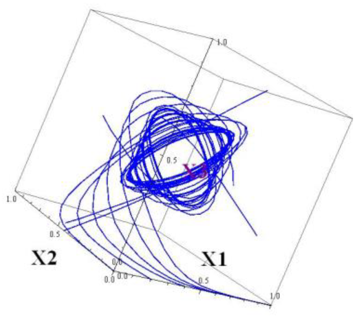
This system has a 4D attractor. It cannot be viewed, but projections to 2D and/or 3D subspaces can. By construction, the projections onto and subspaces looks similar. The projections onto the 3D subspaces ) and () are depicted in Figure 5 and Figure 6.
If a nonzero element is inserted in the matrix , the system immediately may become pre-chaotic, exhibiting a sensitive dependence on the initial data. Testing on the Lyapunov exponents shows these changes.
Several resuts on this matter were published in [4,5,6,7,8,9,10]. The chaotic attractor for 3D systems were discovered
Miscellaneous
GRN are studied not only theoretically, but also having in mind practical applications. The need for managing and control of some GRN stems from the research on the border of medicine and mathematics. In the papers [11], [12] the mathematical problems related to the explanation of genetic issues of leucemia were considered. The authors have constructed the scheme of GRN, which has three attractors. The disease is associated with the tending of the network state to a “bad” attractor. The healthy states are associated with ”normal” attractors. The mathematical problem of treating leucemia is redirecting the system states from a “bad” attractor to a normal one, using adjustable parameters. In the work [13] the authors construct an aging gene regulatory network consisting of the core cell cycle regulatory genes. The process of aging can be characterized by state transitions from the landscape I to II. For networks with a large number of elements the mathematical problem of redirecting a trajectory from one attractor to another is challenging. Although for low dimensional networks this problem can be resolved provided that some needed information is possible. Imagine that there are several attractors and their basins of attractions (all in the invariant set Qn). The current state ( a point in the phase space) is given. The future states are known since the respective trajectory is defined by the initial point. The trajectory goes to a certain attractor. There is a need to redirect the trajectory to another attractor. Sometimes it is possible by changing certain parameters.
For illustration return to system (5). It has the second nullcline in the form of three planes where on the right are the roots of the equation These roots are r1=0.07072, r2=0.5, r3=0.92928. Let the current state of the system be (0.5, 0.2, 0.5). The trajectory from this point goes to the limit cycle of the 2D system (7) at x2=r1. Suppose there is need to redirect this trajectory to the right attractor at x2=r3. This can be done by adjusting a single parameter θ2 to the value 0.42. Only one attractor at x2=0.962948 remains. After the trajectory is sufficiently close to a single attractor at x2=0.962948, the parameter θ2 can be made again 0.5. The system state is now in the basin of attraction of the attractor at x2=r3.
Conclusion (Review of the Literature)
In [14] the role of Lyapunov exponents in detecting chaotic behavior is discussed in the examples of 4D genetic and neural models. In [15] different approaches to the study of GRN are reviewed. In [16] the 2D system was studied. The bifurcation curves in the plane was constructed that separates regions corresponding to two and one attracting critical points. The paper [17] contains the results of the activation case when entries of the regulatory matrix W are positive. It is a rare sample of articles where the n-dimensional system is studied. In particular, the results of [16] are generalized under the assumption that the sum of elements in each row of the matrix W is the same. The book [18] is helpful for researchers active in the study of chaos. It contains interesting suggestions on dynamical systems involved in modeling GRN. The article [19] is a review of several approaches being used to study GRN. The 3D particular system was studied in [20] providing detailed information on critical points and chaotic behavior of solutions. [21] is the application of GRN type systems to managing telecommunication networks. Article [22] is probably the first where GRN type systems appear but they were focused on interrelation of populations of neurons. In [23] the problem of control in 2D GRN type systems was considered. The Gompertz function was chosen to represent nonlinearity. Articles [24], [25], [26] contain results on both genetic and neuronal networks, using Gompertz and logistic nonlinearities. The comparison was made. The titles of the works [27], [28], [29] are quite informative. In the paper [30] the six-order GRN type system was considered. The 3D projections of the obtained attractors are presented. Periodic solutions of 2D, 3D and 4D GRN type systems were considered in [31]. Various examples of biologically induced and GRN type systems were considered in the PhD dissertation by E. Brokan. In the work [33] the authors attempt to understand how the joint dynamics of molecules, cells, genes and pathways may be integrated in the framework of aging biology research contributing to aging. It is proposed that “organismal function is accomplished by the integration of regulatory mechanisms at multiple hierarchical scales, and … the disruption of this ensemble causes the phenotypic and functional manifestations of aging.” Some key examples at different scales are presented that can potentially enrich the understanding of aging. In [34] the authors divide the modeling networks to knowledge-driven and data-driven. This division is discussed within the framework of mechanistic learning. This term refers to the synergistic combination of mechanistic mathematical modeling and data-driven machine or deep learning. This emerging field finds increasing applications in (mathematical) oncology. The single-cell methods are reviewed in [35]. These methods are well suited for GRN investigations. The observation of important factors, resolving gene expression in individual cells can allow subtle behaviours to be detected. An overview of computational approaches to GRN modeling and analysis is presented in the work [36]. The description of processes in living systems through the concept of computation is in focus in the paper [37]. A continuous stream of information receiving and processing by living systems, from single cells to higher vertebrates, is considered as biological computation. The authors highlight the limitations of the current attractor-based framework for understanding computations in biological systems. The authors in [38] review biomedical applications and analyses of interactions among gene, protein and drug molecules for modeling disease mechanisms and drug responses. It is mentioned in the work [39] that one of the “outstanding problems in complexity science and engineering is the study of high-dimensional networked systems and of their susceptibility to transitions to undesired states as a result of changes in external drivers or in the structural properties.” Because of the large number of parameters controlling the state of such complex systems, “the study of their dynamics is extremely difficult.” The authors propose an analytical framework for collapsing complex N-dimensional networked systems into an S+1-dimensional manifold with S << N. In [40] a challenging systems biology problem of searching for possible biochemical networks that perform a certain function is considered. The authors try to elaborate an approach to solve this problem by training a recurrent neural network (RNN) to perform the desired function. The review [41] examines “GRN modeling approaches in aging, encompassing differential equations, Boolean/fuzzy logic decision trees, Bayesian networks, mutual information, and regression clustering. These approaches provide nuanced insights into the intricate gene-protein interactions in aging, unveiling potential therapeutic targets and ARD biomarkers.” The broad spectrum of problems concerning complexity, entropy and statistical learning in nonlinear dynamics is considered in [42]. An impressive list of references contains 207 items. The current problems in complex networks such as network entanglement, order parameter dynamics and model reduction methods for complex network systems are discussed in [43], [44], [45]. In the work [46] the authors declare that ”an accurate prediction of the dynamics seems hardly feasible, because the network is often complicated and unknown. In this work, given past observations of the dynamics on a fixed graph, we show the contrary: Even without knowing the network topology, we can predict the dynamics. Specifically, for a general class of deterministic governing equations, we propose a two-step prediction algorithm.” The problems of morphogenesis as results from the activity of gene networks are discussed in [47]. The fuzzy systems, problems of synchronization, robustness and resilience are considered in [48], [49], [50].
The selection of article for this mini-review is subjective and reflects only the current interest of the author.
Funding
This research received no external funding.
References
- Emmert-Streib, F.; Dehmer, M.; Haibe-Kains, B. Gene regulatory networks and their applications: understanding biological and medical problems in terms of networks. Front. Cell Dev. Biol. 2014; 2, 38. [Google Scholar] [CrossRef]
- Dobzhansky, T. Nothing in Biology Makes Sense except in the Light of Evolution. Am. Biol. Teach. 1973, 35, 125–129. [Google Scholar] [CrossRef]
- Perko, L. Differential Equations and Dynamical Systems, 3rd ed.; Publisher: Springer, New York, 2001. [Google Scholar]
- Kozlovska, O., Sadyrbaev, F. Models of Genetic Networks with Given Properties. WSEAS Transactions on Computer Research, 2022, Vol. 10, 43.-49.lpp. ISSN 1991-8755. 1991; 10. [CrossRef]
- Sandri, M. Numerical Calculation of Lyapunov Exponents. The Mathematica Journal, 1996, 6(3), 78-84.
- Sprott, J. Elegant Chaos. World Scientific, 2010.
- Kozlovska, O., Sadyrbaev, F., Samuilik, I. A New 3D Chaotic Attractor in Gene Regulatory Network, Mathematics., 2024, 12(1), 100, 2024.
- Kozlovska, O. , Sadyrbaev, F. On attractors in systems of ordinary differential equations arising in models of genetic networks. Vibroengineering Procedia, 2023, 49, pp. 136–140. [Google Scholar] [CrossRef]
- Sadyrbaev, F. Example of Chaotic Behavior in Systems of Ordinary Differential Equations Arising in Modeling of Gene Regulatory Networks. CEUR Workshop Proceedings., 2023, 3746, pp. 85–89. 2023, 3746, pp. 85–89 https://ceur. [Google Scholar]
- Kozlovska, O.; Sadyrbaev, F. In Search of Chaos in Genetic Systems. Chaos Theory and Applications, 2024; 6, 13–18. [Google Scholar]
- Cornelius SP, Kath WL, Motter AE (2013) Realistic control of network dynamic. Nat Commun, 1, 1942; 4, 1–9.
- Wang L-Z, Su R-Q, Huang Z-G, Wang X, Wang W-X, Celso G, Lai Y-C (2016) A geometrical approach to control and controllability of nonlinear dynamical networks. Nat Commun, 2016; 7, 11323. [CrossRef]
- Ket Hing Chong, Xiaomeng Zhang, Jie Zheng. Dynamical analysis of cellular ageing by modeling of gene regulatory network based attractor landscape, PLoS ONE 2018 13(6): e0197838. doi.org/10.1371/journal.pone.
- Samuilik, I. Samuilik I., Sadyrbaev F. On a dynamical model of genetic networks. WSEAS Transactions on Business and Economics, 2023, Volume 20, 104-112. [CrossRef]
- M. Alakwaa. Modeling of Gene Regulatory Networks: A Literature Review. J Comp Sys Bio 2014, 1(1): 102. [CrossRef]
- Atslega, S.; Finaskins, D.; Sadyrbaev, F. On a Planar Dynamical System Arising in the Network Control Theory. Mathematical Modelling and Analysis, 3: 21 (3).
- Brokan E.; Sadyrbaev F.. Attraction in n-dimensional differential systems from network regulation theory. Mathematical Methods in Applied Sciences, 2018. [CrossRef]
- Sayama, H. Introduction to the Modeling and Analysis of Complex Systems. Open SUNY textbooks, SUNY Binghampton, 2015.
- N. Vijesh, S. Kumar Chakrabarti, J. Sreekumar. Modeling of gene regulatory networks: A review. J. Biomedical Science and Engineering 6 (2013) 223-231.
- Samuilik, I. , Sadyrbaev F. Modelling three dimensional gene regulatory networks. WSEAS Trans. Syst. Control 2021, 16, 755–763. [Google Scholar] [CrossRef]
- Koizumi Y; Miyamura T.; Arakawa S.; Oki E.; Shiomoto K.; Murata M. Adaptive virtual network topology control based on attractor selection. Journal of Lightwave Technology 2010, 28 (11), 1720-1731. 356. 172.
- Wilson HR, Cowan JD (1972) Excitatory and inhibitory interactions in localized populations of model neurons. Biophys J 12(1):1–24.
- Ogorelova, D. Ogorelova D., Sadyrbaev F., Sengileyev V. Control in Inhibitory Genetic Regulatory Network Models. Contemporary Mathematics, Vol.1, Issue 5, 2020, 393-400.
- Ogorelova, D. Ogorelova, D., Sadyrbaev, F. Comparative Analysis of Models of Genetic and Neuronal Networks. Mathematical Modelling and Analysis, 2024, 29(2), pp. 277–287.
- Samuilik, I. Samuilik, I., Sadyrbaev, F., Ogorelova, D. Comparative Analysis of Models of Gene and Neural Networks. Contemporary Mathematics (Singapore), 2023, 4(2), pp. 217–229.
- Samuilik, I. , Sadyrbaev, F. , Ogorelova, D. Mathematical modeling of three-dimensional genetic regulatory networks using logistic and Gompertz functions. WSEAS Transactions on Systems and ControlThis link is disabled., 2022, 17, pp. 101–107. [Google Scholar]
- Sadyrbaev, F., Ogorelova, D., Samuilik, I. A Nullclines Approach to the Study of 2D Artificial Network. Contemporary Mathematics (Singapore), 2019, 1(1), pp. 1–11.
- Sadyrbaev, F., Sengileyev, V., Silvans, A. On Coexistence of Inhibition and Activation in Genetic Regulatory Networks. AIP Conference Proceedings, 2023, 2849(1), 120004. 2023.
- Sadyrbaev, F. Sadyrbaev, F., Samuilik, I., Sengileyev, V. Biooscillators in Models of Genetic Networks. Springer Proceedings in Mathematics and Statistics, 2023, 423, pp. 141–152 Sadyrbaev, F., Samuilik, I., Sengileyev, V. (2023). Biooscillators in Models of Genetic Networks. In: Vasilyev, V. (eds) Differential Equations, Mathematical Modeling and Computational Algorithms. DEMMCA 2021. Springer Proceedings in Mathematics & Statistics, vol 423. Springer, Cham. [CrossRef]
- Samuilik, I. , Sadyrbaev, F. , Sengileyev, V. Examples of periodic biological oscillators: transition to a six-dimensional system. WSEAS Transactions on Computer ResearchThis link is disabled., 2022, 10, pp. 50–54. [Google Scholar]
- Sadyrbaev, F. , Samuilik, I. , Sengileyev, V. On modelling of genetic regulatory networks. WSEAS Transactions on Electronics, 2021, 12, pp. 73–80. [Google Scholar]
- Brokan E. On a class of systems arising in biomathematics. PhD, Daugavpils University, Daugavpils, November 2021. 20 November.
- Alan A. Cohen , Luigi Ferrucci, Tamàs Fülöp, Dominique Gravel, Nan Hao, Andres Kriete, Morgan E. Levine , Lewis A. Lipsitz, Marcel G. M. Olde Rikkert, Andrew Rutenberg, Nicholas Stroustrup and Ravi Varadhan. A complex systems approach to aging biology. Nature Aging, Vol. 2, July 2022, 580–591. [CrossRef]
- Metzcar J, Jutzeler CR, Macklin P, Köhn-Luque A and Brüningk SC. (2024) A review of mechanistic learning in mathematical oncology. Front. Immunol. 2024 15:1363144. [CrossRef]
- Maizels, RJ. Maizels RJ. A dynamical perspective: moving towards mechanism in single-cell transcriptomics.Phil. Trans. R. Soc. B 379: 2024, 20230049. [CrossRef]
- Barbuti, R., Gori, R., Milazzo P. and Nasti L.A survey of gene regulatory networks modelling methods: from differential equations, to Boolean and qualitative bioinspired models. Journal of Membrane Computing, vol. 2 (2020), 207 - 226.
- Daniel Koch, Akhilesh Nandan, Gayathri Ramesan, Aneta Koseska. Biological computations: Limitations of attractor-based formalisms and the need for transients. Biochemical and Biophysical Research Communications, Vol. 720, 2024, 150069. [CrossRef]
- Rongting Yue and Abhishek Dutta. Computational systems biology in disease modeling and control, review and perspectives. 3: Systems Biology and Applications (2022) 8, 2022. [CrossRef]
- Chengyi Tu, Paolo D'Odorico, Samir Suweis. Dimensionality reduction of complex dynamical systems. iScience, Vol. 24, Issue 1, 2021, 101912. [CrossRef]
- Jingxia Shen, Feng Liu, Yuhai Tu 3 & Chao Tang. Finding gene network topologies for given biological function with recurrent neural network. Nature communications, (2021) 12:3125. [CrossRef]
- José Américo Nabuco Leva Ferreira Freitas * and Oliver Bischof. Computational modeling of aging-related gene networks: a review. Front. Appl. Math. Stat. , Sec. Mathematical Biology, Vol. 10 - 2024. [CrossRef]
- Gilpin, W. Generative learning for nonlinear dynamics. Nat Rev Phys 6, 194–206 (2024). [CrossRef]
- Yiming Huang, Hao Wang, Xiao-Long Ren, Linyuan Lü. Identifying key players in complex networks via network entanglement. Communications physics | (2024) 7:19. [CrossRef]
- Cheng and J.M.A. Scherpen. Model Reduction Methods for Complex Network Systems. Annual Review of Control, Robotics, and Autonomous Systems, Vol. 4:425-453, 2021. [CrossRef]
- Zhigang Zheng, Can Xu, Jingfang Fan, Maoxin Liu, and Xiaosong Chen. Order parameter dynamics in complex systems: From models to data. 0221; 34. [CrossRef]
- Bastian Prassea, and Piet Van Mieghema. Predicting network dynamics without requiring the knowledge of the interaction graph. PNAS 2022 Vol. 119 No. 44 e2205517119. 7119. [CrossRef]
- David, A. David A. Rand , Archishman Raju, Meritxell Sáez, Francis Corson, and Eric D. Siggia. Geometry of gene regulatory dynamics. PNAS 2021 Vol. 118 No. 38 e2109729118. [CrossRef]
- O. Cartagena, S. Parra, D. Muñoz-Carpintero, L. G. Marín and D. Sáez. Review on Fuzzy and Neural Prediction Interval Modelling for Nonlinear Dynamical Systems, in IEEE Access, vol. 9, pp. 23357-23384, 2021. [CrossRef]
- Oriol Artime, Marco Grassia et al. Robustness and resilience of complex networks.
- Dibakar Ghosh, Mattia Frasca, Alessandro Rizzo, Soumen Majhi, Sarbendu Rakshit, Karin Alfaro-Bittner, Stefano Boccaletti. The synchronized dynamics of time-varying networks. Physics Reports, Vol. 949, 2022, Pages 1-63. [CrossRef]
Figure 1.
; ;;
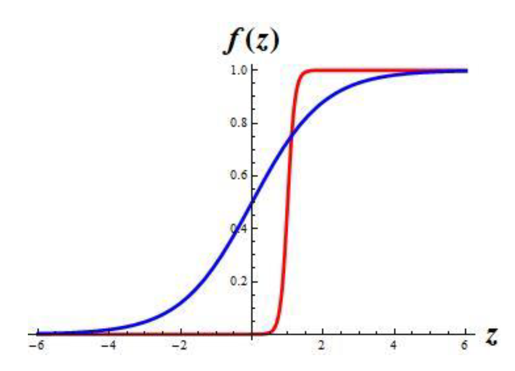
Figure 2.
Nullclines for system (2): 8; ; 8;
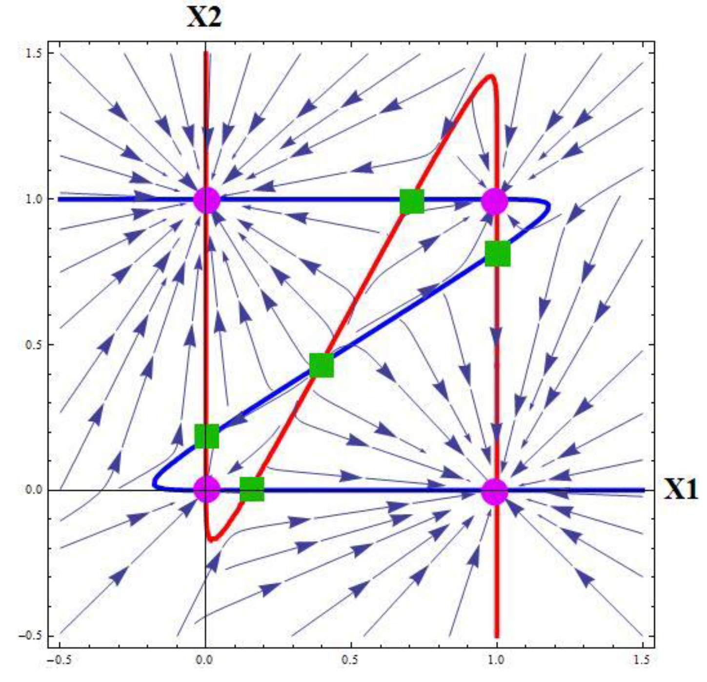
Figure 3.
The nullclines of system (5).
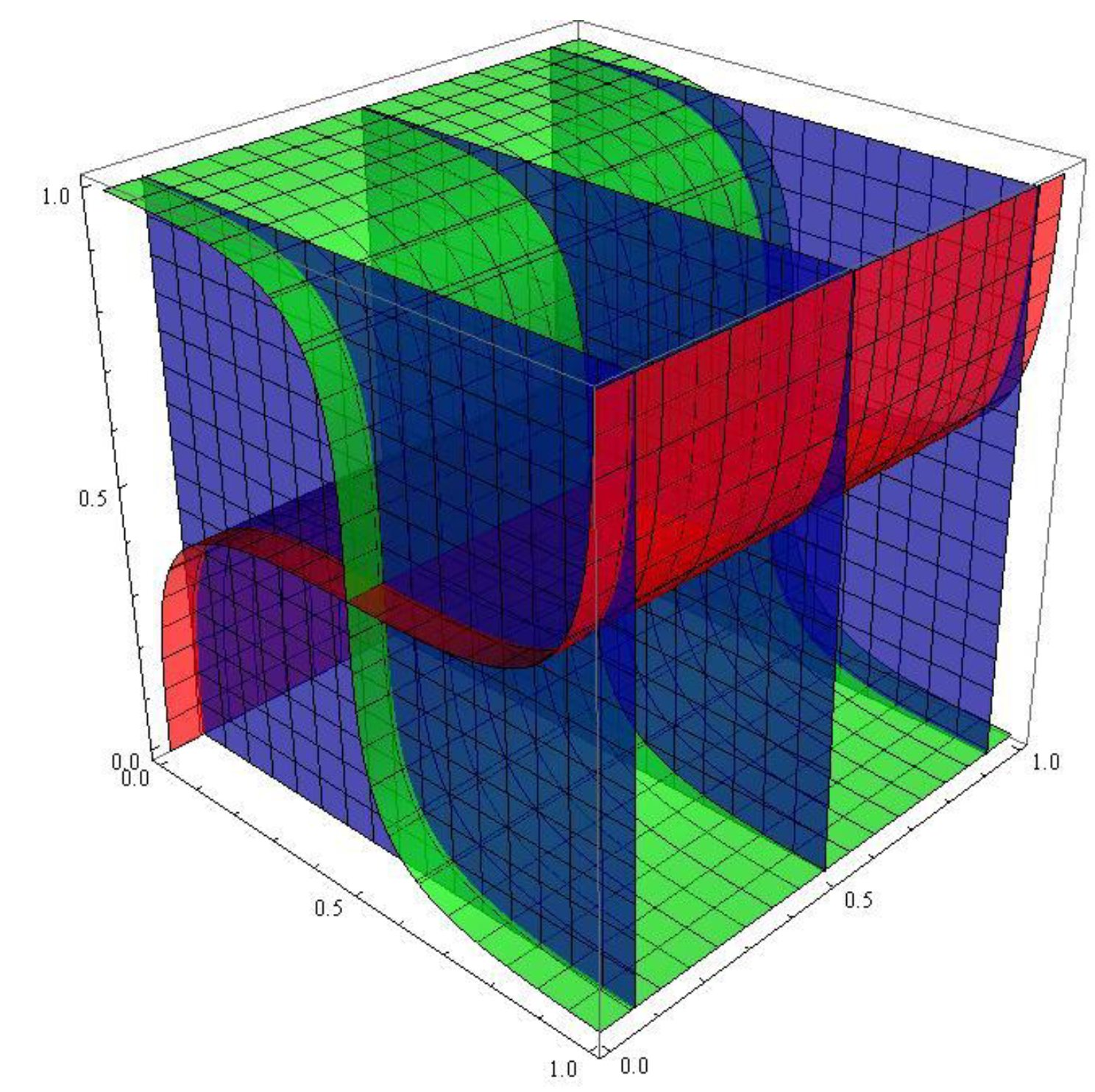
Figure 4.
Several trajectories (orange) of system (5), tending to attractors located on segments (in blue) of the second nullcline.
Figure 4.
Several trajectories (orange) of system (5), tending to attractors located on segments (in blue) of the second nullcline.
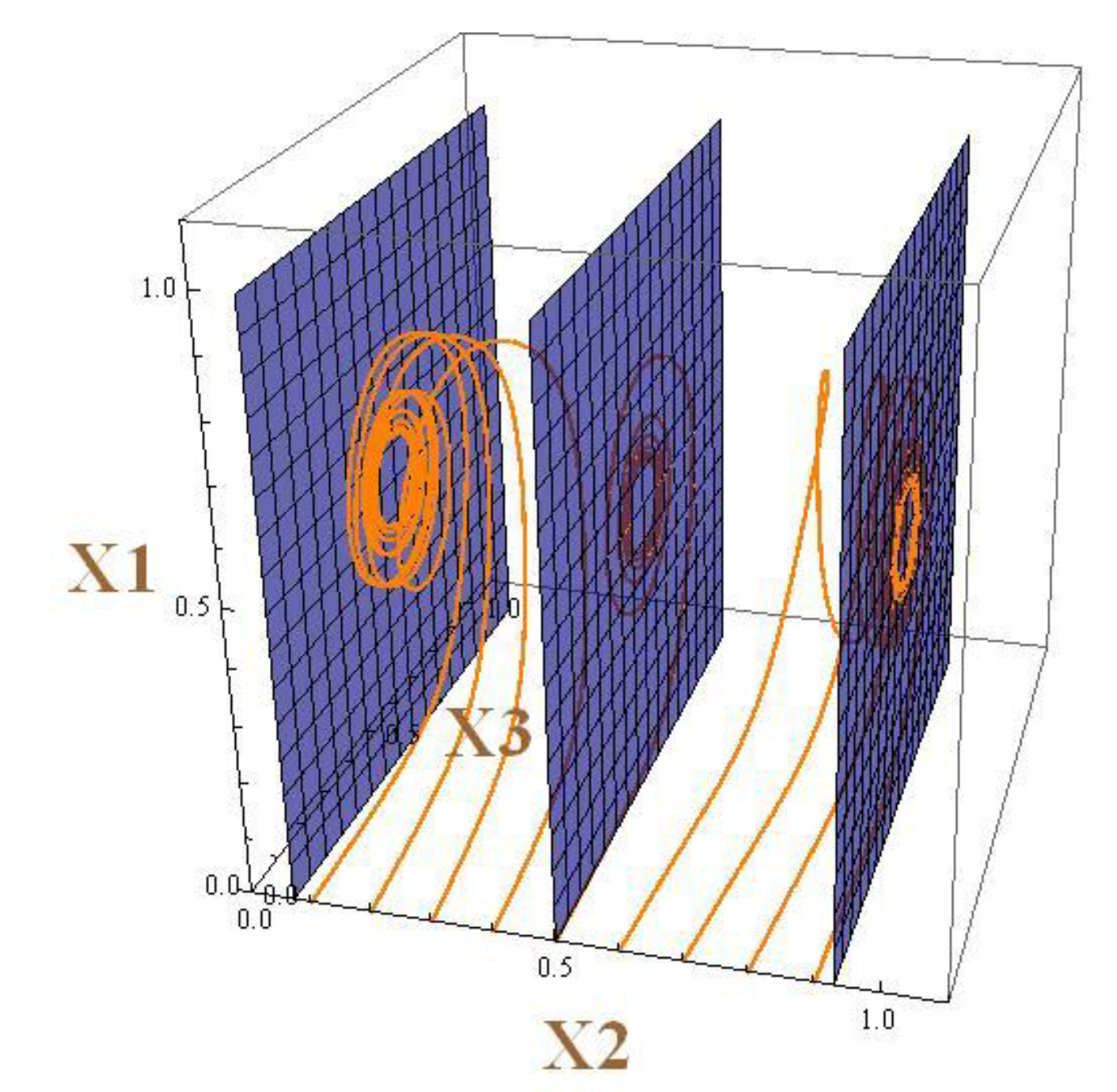
Figure 5.
The projections of attractor in the system (16) onto the 3D subspace .
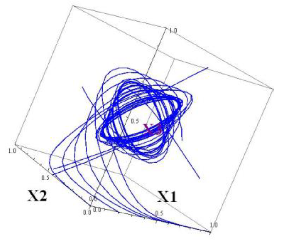
Figure 6.
The projections of attractor in the system (16) onto the 3D subspaces .
Disclaimer/Publisher’s Note: The statements, opinions and data contained in all publications are solely those of the individual author(s) and contributor(s) and not of MDPI and/or the editor(s). MDPI and/or the editor(s) disclaim responsibility for any injury to people or property resulting from any ideas, methods, instructions or products referred to in the content. |
© 2025 by the authors. Licensee MDPI, Basel, Switzerland. This article is an open access article distributed under the terms and conditions of the Creative Commons Attribution (CC BY) license (http://creativecommons.org/licenses/by/4.0/).
Copyright: This open access article is published under a Creative Commons CC BY 4.0 license, which permit the free download, distribution, and reuse, provided that the author and preprint are cited in any reuse.


