
Submitted:
26 February 2025
Posted:
26 February 2025
You are already at the latest version
Abstract
The resistivity method is widely used to address long-term monitoring challenges in fields such as environmental protection, ecological restoration, seawater intrusion, and geological hazard assessment. However, external environmental changes can influence monitoring data, causing inversion results that fail to accurately reflect subsurface variations. Furthermore, the data volume required for such monitoring is several times larger than that for conventional single-point observations, leading to excessively long inversion times and low computational efficiency. To address these issues, we develop a three-dimensional inversion algorithm for the resistivity method incorporating time-lapse constraints. Additionally, MPI parallelization is integrated into the program to enhance computational efficiency. Through the design of theoretical models and the synthesis of data to test the algorithm, the results show that, compared to separate inversion, the shape and values of time-lapse inversion results at different time points are more consistent, maintaining temporal continuity, and the computational efficiency of MPI parallel inversion is greatly improved. Particularly in high-noise environments, time-lapse inversion effectively suppresses background noise interference, reduces false anomalies, and produces results that closely align with the true model, thus confirming the algorithm’s effectiveness and superiority.
Keywords:
Resistivity method
; Time-lapse
; MPI
; Three-dimensional
1. Introduction
In recent years, geophysics has been widely used to monitor subsurface changes. The multi electrode and multi-channel system of the resistivity method allows for the effective collection of large-scale monitoring data, offering significant advantages compared to other geophysical methods. Therefore, time-lapse resistivity inversion has become a hot topic in geophysical inversion.
The Resistivity method has a long history in monitoring. Initially, the international scholar Daily [1] carried out experiments to confirm that resistivity method could monitor the infiltration process of groundwater, but it only involved repeated measurements at different times, without considering the correlation between data at different times. Later, scholars at home and abroad found that normalizing the observation data set before inversion, filtering the false anomalies of the initial data, and then applying traditional inversion algorithm can highlight the small changes in the physical structure underground [2]. Building on normalization research, scholars use the inversion results of background data as a priori model to participate in the inversion calculation of subsequent observation data. This approach improves convergence speed and reduces data fitting errors [3,4,5]. However, these methods do not account for the temporal continuity of physical property changes, making it challenging to accurately reflect subsurface variations. Kim [6] has realized the time-lapse inversion based on the constraint of time-lapse function. This method simultaneously inverts data from different time points while ensuring that the inversion results evolve continuously over time by constraining datasets at different times. However, time-lapse inversion requires simultaneous inversion of monitoring data from multiple time points, demanding substantial memory resources and resulting in inefficiencies.
In this study, we developed a three-dimensional inversion algorithm of the resistivity method, incorporating time-lapse function constraints. We also integrated MPI parallelization into the program to enhance computational efficiency, ensuring that inversion results change continuously over time while significantly improving computational performance. The theoretical model was designed to synthesize data, which confirmed the anti-interference effect of the algorithm.
2. Rationale and Theory
2.1. Three-Dimensional Forward Modeling Algorithm
In this study, the finite difference method is used to implement the three-dimensional forward modeling of resistivity method. According to the forward modeling theory of resistivity method derived from Zhu [7], the partial differential equation satisfied by the point source resistivity method is as follows:
where is the electrical conductivity of rock ore (S·m-1), is the potential array (V), is the electric current density(A·m-2), and is a Dirac function, which specifies the position of the supply point.
The finite difference method is applied to discretize (1), resulting in a large sparse linear system [7], whose matrix form can be expressed as:
where is the coefficient matrix, is the vector that contains information with respect to the field source.
The potential is obtained by solving (2) using the BICGSTAB method. After obtaining the potential, the apparent resistivity is obtained according to (3).
where is the vector that is designed to select the potential at the receiver among all grid node potentials, is the potential difference between the receiving electrodes (V), is the electric current (A), and is the geometric factor.
2.2. Time-Lapse Function
The time-lapse function ensures the continuity of inversion results across different times. In the process of time-lapse inversion, the data at different times are synchronously inverted. Assuming that is the conductivity model at a certain time, then the time-lapse conductivity model can be defined as:
where is the number of observations. At present, there are two calculation methods of time-lapse function: L1 norm and L2 norm [8,9]. In this study, L2 norm method was used for calculation, and the calculation formula is:
is time-lapse function, which is calculated by the difference of the underground conductivity model at the adjacent time. By introducing the time-lapse function into the objective function, the difference of the inversion results at the adjacent time can be reduced by minimizing the objective function, so as to achieve the effect that the underground physical property model changes continuously with time.
2.3. Three-Dimensional Time-lapse Inversion Objective Function
In this study, we use regularized constrained inversion method, which adds model terms to the objective function to constrain, avoiding excessive data fitting and reducing the multiplicity of geophysical inversion solutions. The objective function of regularization constraint inversion is:
The objective function consists of two parts: the data function and the model function . is used to calculate the difference between the observation data and the response data of the inversion result, is used to calculate the smoothness of the model, and is the weight factor of the model function, which is used to adjust the proportion of data function and model function in the objective function.
By introducing the time-lapse function calculated by (5) into (7), the time-lapse inversion objective function can be obtained:
where is the weight factor of the time-lapse function. Expand (8) to get the specific form of the time-lapse inversion objective function:
where is the apparent resistivity data observed at all times, is the forward response function, is the initial model of inversion, is the covariance matrix of the data. The gradient of the objective function can be obtained by calculating the partial derivative of the objective function to :
where is the sensitivity matrices of inversion.
Due to the complexity of underground model and observation data, it is necessary to smooth the gradient of objective function to improve the computational efficiency and stability of inversion. Egbert and Kelbert proposed a simple and efficient method to smooth the gradient of model parameters [10]. The specific transformation formula is derived as follows:
The (10) is transformed by the method above to obtain:
After obtaining through inversion, the model is solved by the following inverse transformation method:
2.4. MPI Parallel Inversion Algorithm
To better reflect the subsurface information, three-dimensional inversion in the resistivity method uses multiple point power sources to improve inversion performance. The corresponding amount of observation data is large, and the original serial inversion program is inefficient. When calculating the forward response, apparent resistivity, and potential at various measuring points for different power supply points, the Jacobian matrix corresponding to each source point during gradient calculation, and the solution of the quasi-forward equation, these tasks are independent of one another. Therefore, the problem can be divided into several independent sub-problems, and parallel computing can enhance the inversion speed and efficiency.
The MPI parallel algorithm significantly improves computational efficiency through the synchronous allocation of tasks across multiple processes. It includes both peer-to-peer and master-slave modes. In the peer-to-peer mode, all processes contribute to completing a portion of the assigned tasks. In the master-slave mode, processes are divided into master and slave processes. The master process is responsible for task allocation, message transmission, and data collection, while the slave processes execute the assigned tasks. In this study, the master-slave mode is selected. Suppose there are 4 field sources, and 10 data points are observed for each field source. N processes are used for calculations using MPI, with each process assigned 40/N field source calculation tasks. Finally, the MPI parallel algorithm is integrated into the inversion algorithm, forming a 3D time-lapse inversion MPI parallel algorithm suitable for combined data from multiple devices in the resistivity method. The MPI parallel inversion flow chart for the resistivity method is shown in Figure 1.
The flow chart can be briefly summarized in the following steps:
1) Input the initial conductivity and set necessary parameters for inversion.
2) The main process collects and assigns tasks to slave processes.
3) Synchronize the calculation of the forward response between the master and slave processes, and continue computing the objective function and gradient.
4) The main process collects the results from all processes.
5) Calculate the update direction and search for the step size.
6) Update the conductivity model.
7) Check if the iteration termination criteria are met. If so, the iteration terminates; if not, the iteration continues.
8) The termination criteria of inversion are when the data misfit is below a predefined threshold or the number of iterations reaches a set limit. The formula for calculating the misfit (root-mean-square, RMS) is:
where is the number of data points.
3. Synthetic Example Tests
3.1. Theoretical Model and Forward Modeling Response
The time-lapse resistivity method is commonly used to monitor the migration process of underground fluid. During the migration process, underground fluid often migrates from one geological unit to another with groundwater. In this study, a time-lapse model is established to simulate the fluid migration process.
Figure. 2 shows the sections of time-lapse model. The anomalous bodies in time-lapse model are two low-resistance prisms. The left prism remains unchanged, while the prism on the right diffuses along the positive direction of the X-axis, simulating the continuous migration of underground fluids over time. The time-lapse model includes three different time points, labeled T1, T2 and T3. The schematic diagram of the model at X-Z and X-Y directions at these three times are shown from left to right. The resistivity of background A is 100 Ω· m, while the resistivity of abnormal bodies B1 and B2 is 10 Ω· m. The size of B1 is fixed, with dimensions of 5 m in the X-direction, 6 m in the Y-direction, and 5 m in the Z-direction. The distance between B1 and B2 is 6m. B2 remains fixed at 6 m in the Y-direction and 5 m in the Z-direction, but its size in the X-direction increases over time, reaching 4 m, 5 m, and 6 m at T1, T2 and T3 respectively.
The same observation system was used for forward modeling of time-lapse model at T1, T2 and T3. Figure 3 is a schematic diagram of the observation system. The three-pole device is used for measurement on the ground surface. The electrodes are arranged as a rectangular square array, the red triangle is the position of the transmitting electrode, the blue dot is the position of the receiving electrode, and the black solid line box is the projection of the anomalous bodies B1 and B2 on the ground surface. When each transmitting electrode is powered, all adjacent receiving electrodes in the X direction received to ensure that enough information in the three-dimensional space is obtained. Gaussian-random errors of 5%, 5% and 20% were added to the observation data at T1, T2 and T3 respectively, which can simulate the situation that the data at a certain time in the actual work was greatly disturbed by noise. At last, there were a total of 194 sources, with 23760 data were obtained at a single time, and a total of 71280 data were obtained at three times.
3.2. MPI Parallel Calculation Efficiency
To evaluate the computational efficiency of the three-dimensional MPI parallel inversion in the time-lapse resistivity method. Taking the above synthetic data as an example, with consistent grid division, inversion of the initial model, and observation data errors, the program was executed using 5, 10, and 20 processes, respectively, and the time of the serial program is compared. Table 1 shows the running time of the serial program and the MPI parallel program.
As shown in Table 1, the relative acceleration ratio between MPI parallel program and serial programs is not an integer multiple relationship, which is caused by two reasons. Firstly, during the execution of parallel programs, data transfer between processes takes up time, resulting in time consumption. Secondly, only processes with high computational complexity such as forward response, objective function, and gradient need to use MPI parallel computing, the other processes don’t need to use MPI parallel program. Overall, the computational efficiency of MPI parallel program decreases as the number of processes increases.
3.3. Analysis of Inversion Results
We performed both separate inversion and time-lapse inversion on the synthesized data. Figure 4 and Figure 5 show the sections at Z = 8m and Y = 0m for the separate inversion and time-lapse inversion results, respectively. The black solid line in the figures represents the true location of the anomalous bodies.
In the analysis of the results shown in Figure 4 and Figure 5, it is evident that the time-lapse inversion results are more similar in shape and resistivity values for anomalous bodies B1 and B2 at all three time points, compared to the separate inversion results.
Comparing the separate inversion results of the three times with the time-lapse inversion. At T1, the time-lapse inversion better approximates the shape and resistivity of anomalous body B2 compared to the separate inversion. At T2, there is no significant change in the shape or resistivity of anomalous bodies B1 and B2 between the time-lapse and separate inversions. At T3, the separate inversion results are heavily influenced by noise, distorting the shapes of B1 and B2 and introducing false anomalies around the anomalous bodies. In contrast, the time-lapse inversion significantly reduces these distortions and eliminates most of the false anomalies.
To further assess the constraint effect of the time-lapse function, we computed the difference between adjacent time points for both the separate inversion and time-lapse inversion results, as shown in Figure 6 and Figure 7. The black solid line represents the model from the previous time step, and the area between the black solid line and the dotted line highlights the model changes relative to the previous time.
It can be seen from the Figure 6 and Figure 7 that the resistivity difference between adjacent times is smaller after time-lapse inversion. At the Z = 8m sections, the resistivity of T2-T1 model significantly decreases in the real change area after separate inversion, and the reduction range is larger than that in the real change area. The resistivity of T3-T2 model changes disorderly, which is inconsistent with the real change area, which is mainly caused by the influence of high noise at T3. After time-lapse inversion, the variation ranges of resistivity of T2-T1 and T3-T2 models are on the right side of the real variation area, and the variation value is smaller, while the variation range of resistivity of T3-T2 model is more regular. At the Y = 0m section, the resistivity of T2-T1 and T3-T2 decrease around B2 after separate inversion, and the variation range is larger than the real variation region. After time-lapse inversion, the variation range of resistivity is smaller, and it is concentrated in the upper right of the real variation region.
To sum up, the inversion results of time-lapse inversion at adjacent times are more similar in value form, and can still reflect the change of underground resistivity under high noise interference.
4. Conclusions
In this study, a three-dimensional inversion of the time-lapse resistivity method based on time-lapse function constraint theory was implemented, and MPI parallel design was incorporated into the program.
Using synthetic data from the theoretical model, both separate inversion and time-lapse inversion were conducted to test the program. The MPI parallel design significantly reduced the program runtime, which is critical for geophysical monitoring. Comparing the separate inversion results with the time-lapse inversion results, it was found that the difference between the inversion results at adjacent times is smaller after time-lapse inversion, indicating that the shape of the inversion results at different times is closer to the true resistivity values. Especially in high-noise environments, the time-lapse inversion effectively suppresses false anomalies at the boundaries and background of the model, demonstrating strong resistance to interference and the ability to reflect changes in underground resistivity. Overall, the parallel inversion program for time-lapse resistivity methods has been shown to be reliable and superior.
Author Contributions
Conceptualization, D.Z.; methodology, D.Z. and Y.Y.; software, D.Z; validation, D.Z., L.W.; writing-original draft preparation, D.Z.; writing-review and editing, D.Z., L.W.; supervision, Y.Y. All authors have read and agreed to the published version of the manuscript.
Funding
This research was funded by The National Oil and Gas Basic Geological Survey Project of China (No. DD20240052).
Data Availability Statement
Not applicable.
Conflicts of Interest
The authors declare no conflicts of interest.
References
- Daily, W., A. Ramirez, et al. Electrical resistivity tomography of vadose water movement. Water Resources Research 1992, 28, 1429–1442. [Google Scholar]
- Cassiani, G., V. Bruno, et al. A saline trace test monitored via time-lapse surface electrical resistivity tomography. Journal of Applied Geophysics 2006, 59, 244–259. [Google Scholar]
- LaBrecque, D.J. and X. Yang. Difference Inversion of ERT Data:a Fast Inversion Method for 3-D In Situ Monitoring. Journal of Environmental and Engineering Geophysics 2001, 6, 83–89. [Google Scholar] [CrossRef]
- Oldenborger, G.A., M. Knoll, and D.J. LaBrecque. Time-lapse ERT monitoring of an injectionwithdrawal experiment in a shallow unconfined aquifer. Geophysics 2007, 72, 177–187. [Google Scholar] [CrossRef]
- Miller, C.R., P. S. Routh, et al. Application of Time-Lapse ERT Imaging to Watershed Characterization. Geophysics 2008, 73, 7–17. [Google Scholar] [CrossRef]
- Kim, K.J. and I.K. Cho. Time-lapse inversion of 2D resistivity monitoring data with a spatially varying cross-model constraint. Journal of Applied Geophysics 2011, 74, 114–122. [Google Scholar] [CrossRef]
- Zhu, D., H. Tan, et al. Three-Dimensional Joint Inversion of the Resistivity Method and Time-Domain-Induced Polarization Based on the Cross-Gradient Constraints. Applied Sciences.
- Kim, J.H., R. Supper, et al. Four-dimensional inversion of resistivity monitoring data through Lp norm minimizations. Geophysical Journal International 2013, 195, 1640–1656. [Google Scholar] [CrossRef]
- Loke, M.H., T. Dahlin, and D.F. Rucker. Smoothness-constrained time-lapse inversion of data from 3D resistivity surveys. Near Surface Geophysics 2013, 12, 5–24. [Google Scholar] [CrossRef]
- Egbert, G.D. and A. Kelbert. Computational recipes for electromagnetic inverse problems. Geophysical Journal International 2012, 189, 251–267. [Google Scholar] [CrossRef]
Figure 1.
MPI parallel inversion flow chart of the resistivity method.

Figure 2.
The sections of time-lapse model. The three columns from left to right represent the models at three times. The top panels (a) are schematic diagrams in the X-Z direction at T1, T2 and T3, and the bottom panels (b) are schematic diagrams in the X-Y direction at T1, T2 and T3. The resistivity value of background A is 100 Ω· m, and the resistivity of abnormal bodies B1 and B2 is 10 Ω· m. The direction of the red arrow represents the change direction of B2.
Figure 2.
The sections of time-lapse model. The three columns from left to right represent the models at three times. The top panels (a) are schematic diagrams in the X-Z direction at T1, T2 and T3, and the bottom panels (b) are schematic diagrams in the X-Y direction at T1, T2 and T3. The resistivity value of background A is 100 Ω· m, and the resistivity of abnormal bodies B1 and B2 is 10 Ω· m. The direction of the red arrow represents the change direction of B2.
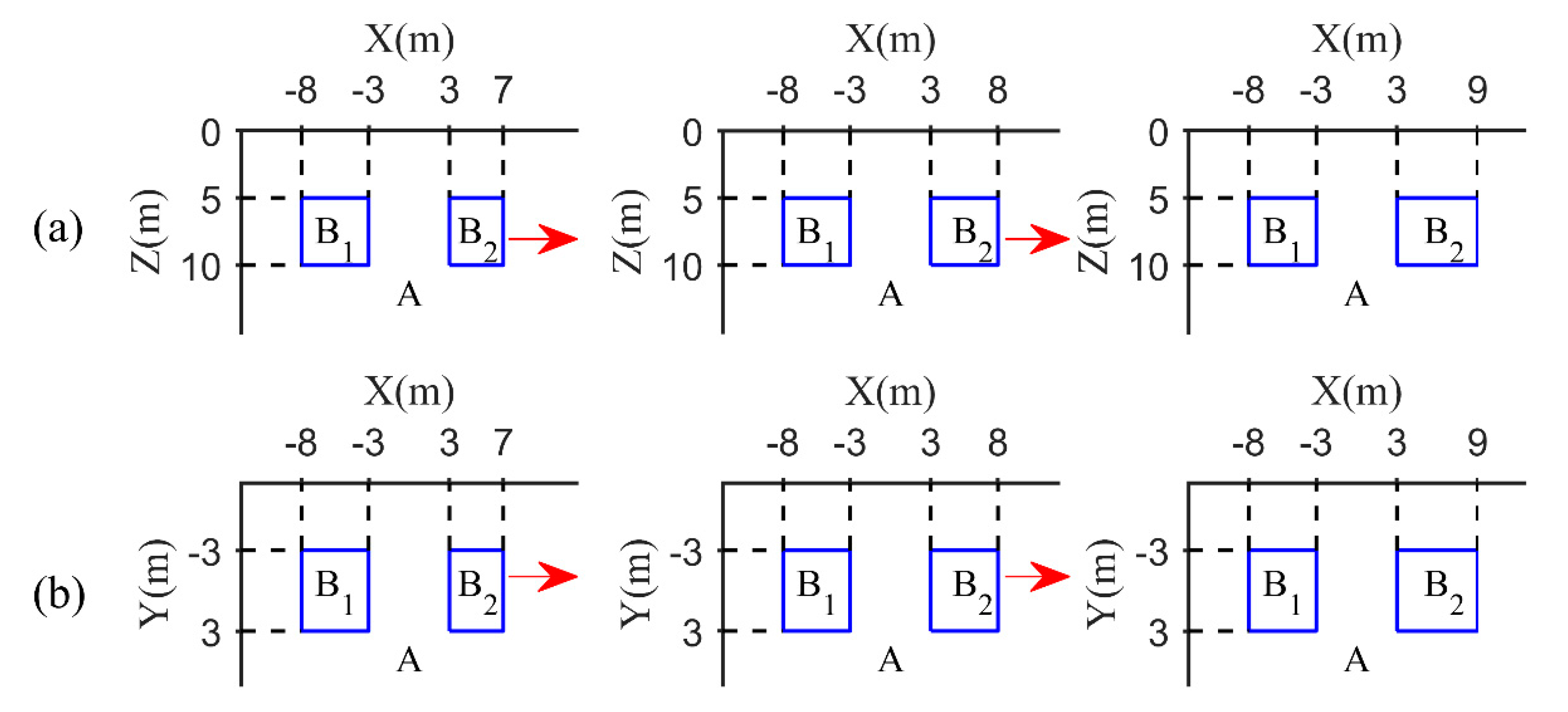
Figure 3.
Schematic diagram of the observation system. The red circle triangles denote transmitters, the blue dots denote receivers, and the black rectangle denotes the projection of the prism on the surface.
Figure 3.
Schematic diagram of the observation system. The red circle triangles denote transmitters, the blue dots denote receivers, and the black rectangle denotes the projection of the prism on the surface.
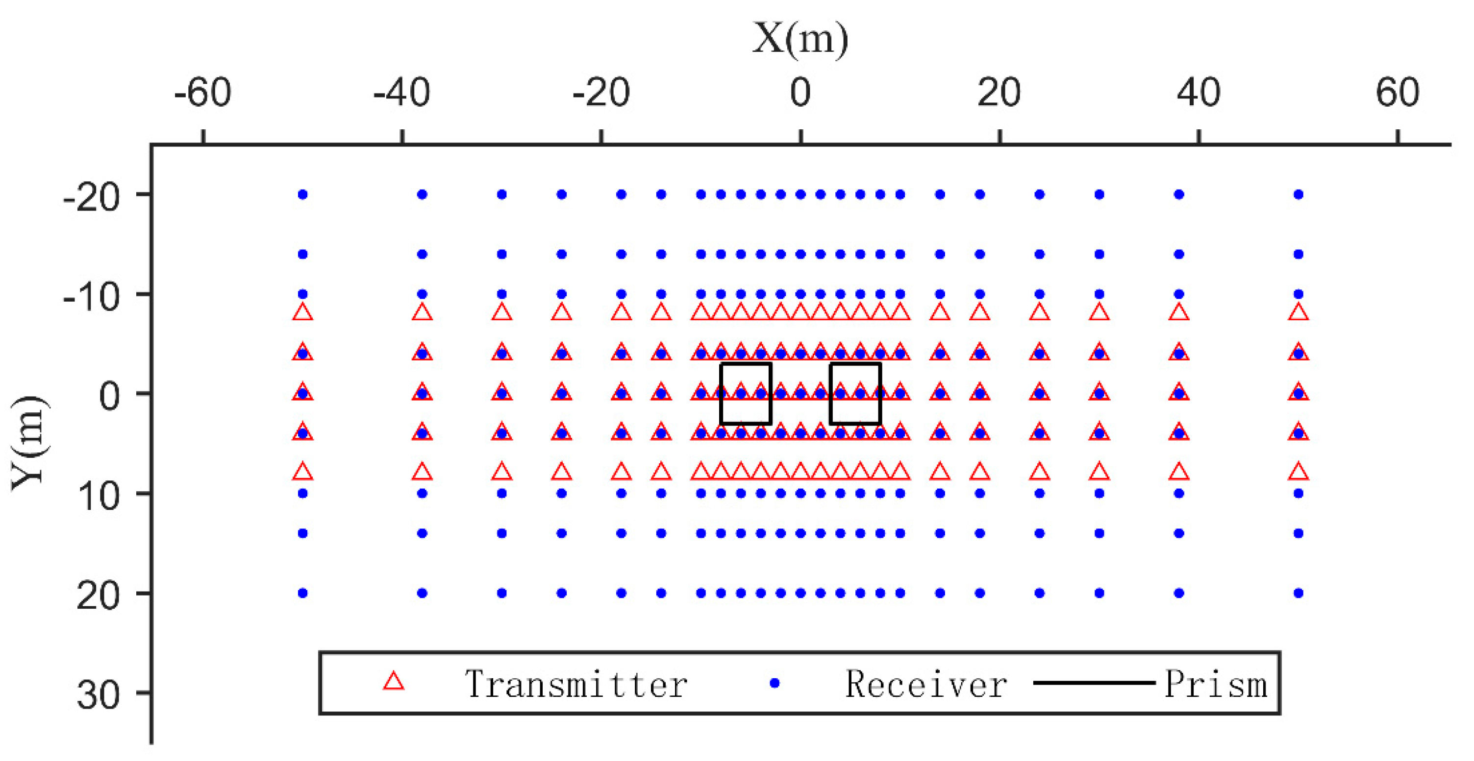
Figure 4.
The sections at Z = 8m from separate inversion and time-lapse inversion of synthetic data. The separate inversion results are shown in the first column, and the time-lapse inversion results are shown in the second column, the top to down panels of (a), (b), (c) are schematic diagrams at T1, T2 and T3 respectively.
Figure 4.
The sections at Z = 8m from separate inversion and time-lapse inversion of synthetic data. The separate inversion results are shown in the first column, and the time-lapse inversion results are shown in the second column, the top to down panels of (a), (b), (c) are schematic diagrams at T1, T2 and T3 respectively.
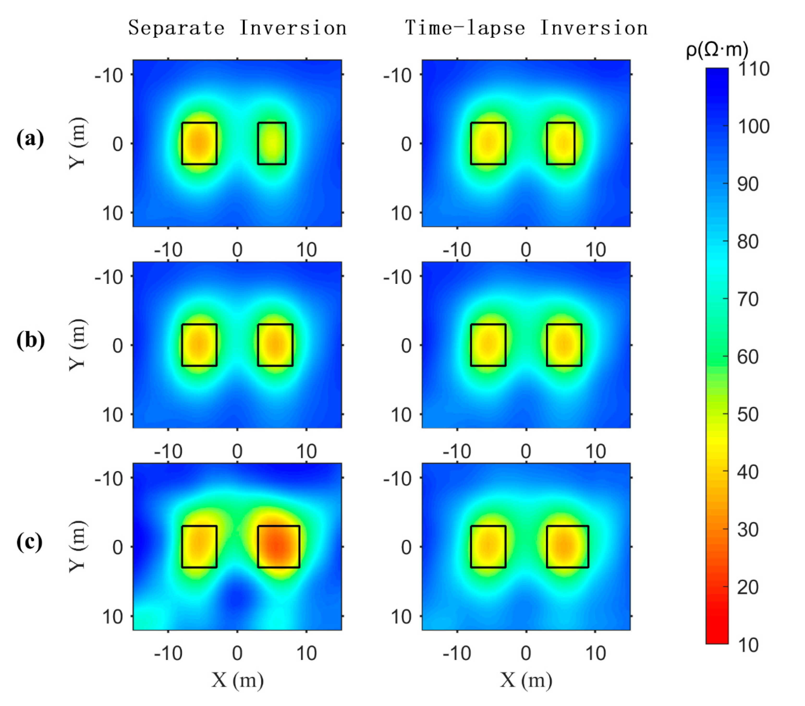
Figure 5.
The sections at Z = 8m from separate inversion and time-lapse inversion of synthetic data. The separate inversion results are shown in the first column, and the time-lapse inversion results are shown in the second column, the top to down panels of (a), (b), (c) are schematic diagrams at T1, T2 and T3 respectively.
Figure 5.
The sections at Z = 8m from separate inversion and time-lapse inversion of synthetic data. The separate inversion results are shown in the first column, and the time-lapse inversion results are shown in the second column, the top to down panels of (a), (b), (c) are schematic diagrams at T1, T2 and T3 respectively.
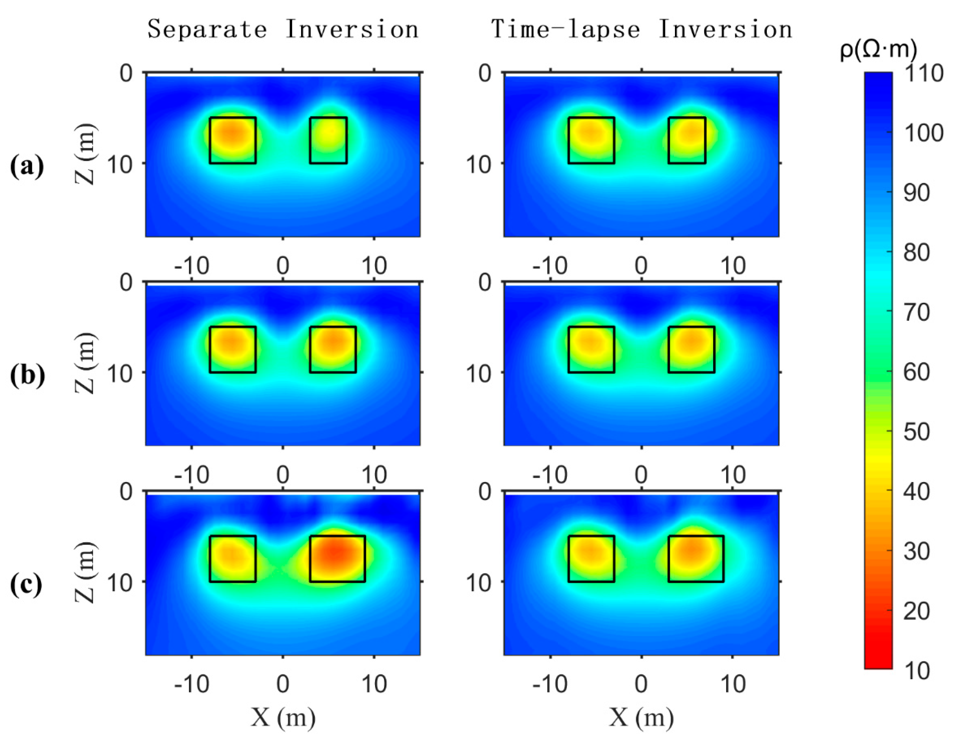
Figure 6.
The sections of resistivity difference with adjacent time at Z = 8m in the results of separate inversion and time-lapse inversion of synthetic data. The top panels (a) are schematic diagrams of T2 – T1, the bottom panels (b) are schematic diagrams of T3 – T2.
Figure 6.
The sections of resistivity difference with adjacent time at Z = 8m in the results of separate inversion and time-lapse inversion of synthetic data. The top panels (a) are schematic diagrams of T2 – T1, the bottom panels (b) are schematic diagrams of T3 – T2.
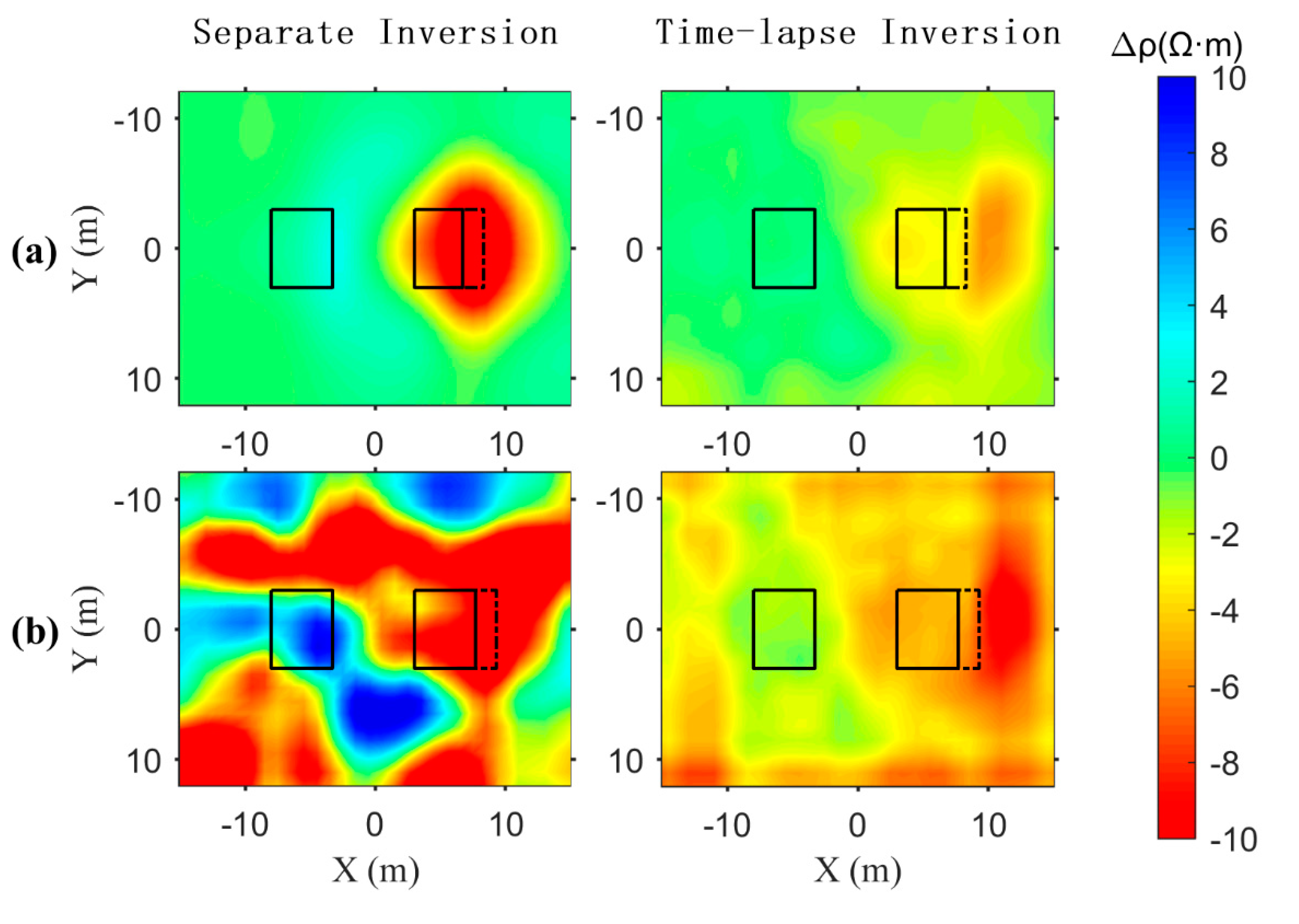
Figure 7.
The sections of resistivity difference with adjacent time at Y = 0m in the results of separate inversion and time-lapse inversion of synthetic data. The top panels (a) are schematic diagrams of T2 – T1, the bottom panels (b) are schematic diagrams of T3 – T2.
Figure 7.
The sections of resistivity difference with adjacent time at Y = 0m in the results of separate inversion and time-lapse inversion of synthetic data. The top panels (a) are schematic diagrams of T2 – T1, the bottom panels (b) are schematic diagrams of T3 – T2.
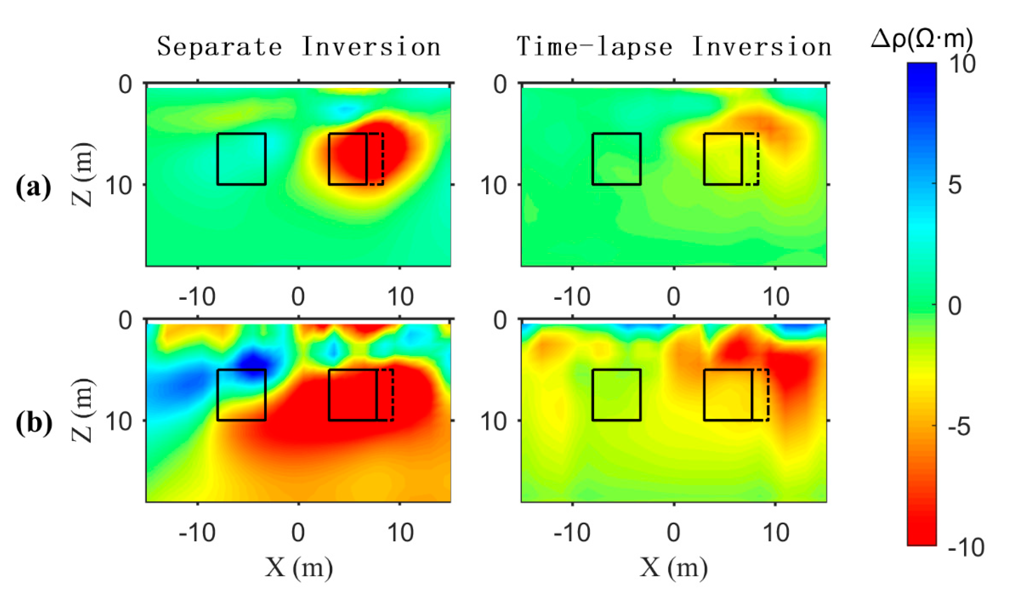

Table 1.
Comparison of the running time of the serial program and the MPI parallel program.
| Type of program | Number of processes | Running Time / Minutes |
Acceleration ratio |
|---|---|---|---|
| Serial program | 1 | 487.26 | 1 |
| MPI parallel program | 5 | 124.3 | 3.92 |
| 10 | 64.62 | 7.54 | |
| 20 | 36.77 | 12.98 |
Disclaimer/Publisher’s Note: The statements, opinions and data contained in all publications are solely those of the individual author(s) and contributor(s) and not of MDPI and/or the editor(s). MDPI and/or the editor(s) disclaim responsibility for any injury to people or property resulting from any ideas, methods, instructions or products referred to in the content. |
© 2025 by the authors. Licensee MDPI, Basel, Switzerland. This article is an open access article distributed under the terms and conditions of the Creative Commons Attribution (CC BY) license (http://creativecommons.org/licenses/by/4.0/).
Copyright: This open access article is published under a Creative Commons CC BY 4.0 license, which permit the free download, distribution, and reuse, provided that the author and preprint are cited in any reuse.