Submitted:
21 February 2025
Posted:
21 February 2025
You are already at the latest version
Abstract
The potential of machine learning (ML) models for predicting crystallographic symmetry information from single-phase powder X-ray diffraction (XRD) patterns is investigated. Given the scarcity of large, labeled experimental datasets, we train our models using simulated XRD patterns generated from crystallographic databases. A key challenge in developing reliable diffraction-based structure-solution tools lies in the limited availability of training data and the presence of natural adversarial examples, which hinder model generalization. To address these issues, we explore multiple training pipelines and testing strategies, including evaluations on experimental XRD data. We introduce a contrastive representation learning approach that significantly outperforms previous supervised learning models in terms of robustness and generalizability, demonstrating improved invariance to experimental effects. These results highlight the potential of self-supervised learning in advancing ML-driven crystallographic analysis.
Keywords:
diffraction
; crystallography
; machine learning
; self-supervised learning
; representation learning
1. Introduction
Determining an unknown crystal structure and, hence, identifying a new chemical compound (usually called “crystallographic phase”) from X-ray or neutron powder diffraction data is an inverse problem that requires experienced users to make several strategic choices across multiple steps in the course of structure determination. The typical pipeline following the measurement of intensities from an appropriate laboratory or high-resolution X-ray (or neutron) diffractometer and radiation source starts with binning the diffraction pattern, describing the background, and then identifying the so-called Bragg peak positions from elastic coherent scattering. This is followed by indexing the pattern to identify the crystal system, the unit cell and then narrowing down the number of potential space groups, based on which a structure-solving algorithm suggests candidate structures, eventually improved or rejected by (Rietveld) structure refinement [1]. Depending on the chemical nature of the sample, the candidate structures are usually determined using approaches going under the names Direct Methods or Patterson Method [2], or other methods such as Simulated Annealing [3], Genetic Algorithms [4], Charge Flipping [5], etc. By doing so, the generally complex structure factors are found which reconstruct (upon Fourier transformation) the measured intensities, so the model may be compared to the real world that has been measured.
The aforementioned “pipeline” carried out by human beings has allowed for a huge number of structure determinations (by solving the “phase problem”, that is, determining the atomic positions in real space) but the exact course is difficult to predict from a more general perspective since it depends on the chemical nature, on the structural complexity, on human skills, and so forth. That being said, specific choices must be taken which may be considered as iterative informed guesses, most often also based on additional sources of information. This is particularly true if more than one chemical species (multiple-phase diffraction patterns) are being looked at, so the indexing step faces a tremendous challenge to begin with: which of the Bragg peaks belongs to which phase? It may therefore be a good idea to utilize data-driven machine learning models that can directly generate or identify or at least estimate candidate crystallographic structures based on the measured data.
Typically, a supervised machine learning model needs large amounts of labelled data which, in our specific case, relates to experimental diffraction patterns and the corresponding structure information of the measured sample in order to make accurate predictions. Models trained on limited data can be vulnerable to “natural adversarial examples”, i.e., naturally occurring instances that unintentionally cause a model to make incorrect predictions. Likewise, such models may also make predictions based on spurious correlations in the data rather than useful features. While limited data availability is a persistent challenge in many experimental sciences, machine-learning models have demonstrated remarkable flexibility in adapting to these constraints. Despite initial hurdles, models like AlphaFold [6] have revolutionized their respective fields by leveraging innovative training strategies and structural priors, ultimately surpassing traditional approaches. Inspired by such advancements, we explore how data-driven models can be designed to tackle the complexities of crystallographic structure prediction
From a statistical point of view, acquiring experimental data representative enough to model the joint distribution of the diffraction patterns (including instrumental effects) and the corresponding structure information is intractable because one cannot quickly synthesize and re-measure hundreds of thousands of solid-state chemical compounds. We can, however, extract experimental crystal-structure information already stored as Crystallographic Information Files (CIF) being part of large-scale crystal-structure databases such as the Crystallography Open Database (COD) or the Inorganic Crystal Structure Database (ICSD). Given that the data contained in those CIF files are accurate and idealized (that is, almost free of any measuring inaccuracies), experimental diffraction patterns may be straightforwardly simulated. It is important to note, however, that designing a machine-learning model trained with simulated data of known structures which eventually processes experimental diffraction patterns corresponds to a cyclic problem.
This issue can, at least to a certain extent, be circumvented by using models that take manual or “handcrafted” features of the experimental diffraction patterns as the input. We shall later show that for specific tasks such as indexing and crystal-system determination such models can potentially outperform well-known existing search-based, non-data-driven algorithms like NTREOR [7]. However, models trained on handcrafted features (typically chosen by a trained human being) are time-consuming and difficult to evaluate since such models require some “pre-processing” steps (e.g., peak detection), making it difficult to debug mistakes. In other words, this real-world component makes the model vulnerable to adversarial effects inherently present in any experimental measurement. More importantly, such models and the features used by them do not generalize over different tasks, and therefore cannot be used to build an end-to-end structure prediction model.
To fulfill the ultimate vision of reliably using data-driven ML models for structure solutions from powder diffraction patterns, we need to ensure that the underlying architecture is both scalable and capable of generalizing across different tasks. Additionally, it is crucial to minimize vulnerabilities introduced by pre-processing steps, enabling the model to function with minimal human intervention. Therefore, our goal is to use the entire diffraction pattern as input and design a model that inherently learns robust feature representations. To achieve this, the model must be invariant to variations in the input caused by sample or instrumental effects and noise while remaining sensitive to variations arising from structural differences. Simply put, changes in the input should only influence the prediction if they correspond to a genuine structural difference in the measured crystallographic structure. For this, we investigate neural network architectures with training pipelines inspired by recent advancements in semi- and self-supervised representation learning. We believe this approach will facilitate previously unseen robustness against “natural adversarial examples” arising from noise to experimental variations of the diffraction pattern input, and one needs to ensure that both the model architecture and the training methodology are suitable to reach this goal.
To focus and streamline our work, we limit our scope to prediction tasks, specifically classifying the crystal system, extinction group, and space group from diffraction patterns of predominantly single-phase samples. We explore model architectures, testing standards, and training methodologies to enhance model reliability and generalizability.
2. Previous Works
The idea of training machine-learning models for identifying crystallographic phase information such as crystal system, lattice parameters, and space groups, as well as estimating non-crystallographic properties like electronic band gap, formation energy, etc., is not entirely new. For example, Suzuki et al. [8] studied the use of machine-learning models such as Support Vector Machines, Random Forests, and Randomized Decision Trees trained with handcrafted features such as the position of the first ten low-angle (2θ) peaks and the number of peaks in the 2θ range of 0–90°. The data for training and testing were generated from simulated powder-diffraction patterns stemming from CIF files taken from ICSD, using the aforementioned handcrafted features. As typical for data-driven models, the test set was a part of the entire dataset kept separate from the data used for training the model. Suzuki et al. [8] reported a crystal-system classification accuracy of 90% and a space-group classification accuracy of about 80.5%. The performance reported over experimental data, however, was limited to two rather typical laboratory XRD measurements of Ca1.5Ba0.5Si5N6O3 and BaAlSi4O3N5:Eu2+ but space-group classification failed for both. We adopt this approach of using handcrafted features in one of our baseline experiments.
Park et al. [9] proposed treating the entire powder diffraction pattern as a one-dimensional picture using a Convolutional Neural Network (CNN) trained on single-phase simulated diffraction patterns of crystal structures from the ICSD database. This was intended to predict the crystal system, the extinction group (derived from systematic absences or extinctions), and the space group. The authors proposed a data-generation pipeline using a set of fixed parameters such as the structure factor, the multiplicity, the Lorentz polarization factor, and a set of randomly selected parameters involved in the pseudo-Voigt peak profile function, the Caglioti parameters [10], and the coefficients of the background polynomial. Owing to this, the proposed CNN internally learned a representation of the diffraction pattern as opposed to the models presented by Suzuki et al. [8] and its handcrafted features. When tested on generated data using the aforementioned data-generation pipeline on a sub-set of ICSD crystal structures not used in training, the paper reported 94, 83.8, and 81.1% accuracy for crystal-system, extinction-group, and space-group classification, respectively. For testing on experimental data, Park et. al. [9] also reported their model’s prediction on Ca1.5Ba0.5Si5N6O3 and BaAlSi4O3N5:Eu2+. Similar to Suzuki et al. [8], the predictions also failed for both extinction and space groups. Although the model by Park et al. [9] learned better representations due to random parameters of the data-generation pipeline, the authors did not explicitly investigate the model’s invariance as regards experimental effects. In addition, the rather limited experimental testing makes it difficult to analyze the model’s robustness for practical use.
Lee et al. [11] expanded on some of the ideas by Park et al. [9], first by including training Fully Convolutional Neural Networks (FCNNs) as well as a Vision Transformer-inspired neural network for predicting extinction and space group for single-phase simulated diffraction patterns from the ICSD and the Materials Project (MP) dataset and, second, neural network regression models trained on the non-experimental MP data to estimate DFT-calculated band gap, formation energy, and the energy above the convex hull. Although the authors reported close to state-of-the-art (SOTA) performances, they also did not perform extensive tests for the model’s robustness over natural adversarial examples.
Oviedo et al. [12] proposed a more representative simulation pipeline that models the evolution of a thin-film XRD experiment by modifying the XRD data in terms of pattern shifting, peak scaling, and peak elimination, an approach usually dubbed as “augmentation” in this simulative context. They measured 85 thin-film experimental XRD patterns of known structures belonging to seven different space groups, including perovskite-like materials such as lead halides (Pmm), tin halides (I4/mcm), Cs-Ag-Bi bromide double perovskites (Fmm), and Bi and Sb halides (Pm1, Pc, P21/c, P63/mmc). The goal of Oviedo et al. [12] was to classify the XRD patterns into the seven aforementioned space groups, and the data-augmentation strategy was designed such that the simulated data used for training accurately fitted the measured thin-film X-ray diffraction (XRD) patterns. The paper reported an accuracy of about 99 and 80% on a simulated/experimental test set for the seven space-group classification problem; admittedly, this corresponds to a much simpler task compared to other works.
Salgado et al. [13] trained a neural network model for classifying the space group using a combination of simulated and experimental data. The simulated XRD data consisting of 1.2 million training patterns were generated from ICSD structures using a set of Caglioti parameters and noise implementations, and the experimental XRD patterns (908 patterns) were collected from the RRUFF Dataset. The authors evaluated space-group classification accuracy across models trained on various sets of data. Particularly, they trained neural network models on simulated data as well as a combination of simulated data and half of the experimental data, while using the rest for testing. The best-case accuracy reported for their models trained entirely using simulated data was 66%, which increased to 77% when half the experimental data were added for training. Hence, Salgado et al. [13] addressed the challenges involved when training machine learning models on simulated data that can be robust enough to work on experimental data.
Lolla et al. [14] introduced a semi-supervised deep learning model for classifying powder neutron diffraction patterns into 14 Bravais lattices and 144 space groups. The model leveraged simulated diffraction patterns as labeled data while exploring the use of partially labeled datasets during training. Despite achieving state-of-the-art results on simulated test datasets, the study did not incorporate real experimental data as labeled training examples, nor did it evaluate the model’s performance on real experimental datasets. This limitation highlights a gap in generalizability to real-world XRD patterns, which may include experimental noise and other complexities not captured in simulations. However, this work introduced an interesting idea of using the Discriminator of a Generative Adversarial Network [15] to predict the Bravais lattice and space groups. This concept introduces the possibility of incorporating experimental XRD patterns into the unsupervised training modes of the Discriminator in future work, thereby potentially improving its applicability to real-world data.
In this paper, we adopt a self-supervised representation learning strategy, which relies entirely on simulated data for training. We have been inspired by the aforementioned contributions, laying the groundwork for identifying and addressing the challenges in learning representations from simulated diffraction patterns that can be generalized well enough to be used in real life.
3. Crystallographic and Diffraction Data
The data-driven models discussed in this paper are trained and tested using data simulated from known crystallographic structures. It is important to outline the details of the simulation process to provide context for the subsequent analysis.
The general functional form of the calculated intensity at the th position of the diffraction pattern for a given crystal structure is given as:
where .
Here is the scale factor, is the reciprocal lattice vector as expressed by the hkl triple, are the Lorentz and polarization factors, the multiplicity factor, is the structure factor, is the profile function, and is the product of the absorption and extinction factors. The structure factor contains all the crystallographic information about the atoms j and their relative positions in the unit cell, while the set of all dictates the symmetry of the unit cell. Here is the multiplicity of the atomic position, is the atomic form factor, is the position vector, and B is the (isotropic) thermal displacement factor, also going under the name Debye–Waller factor.
We use the Inorganic Crystal Structure Database (ICSD) which consists of over 200,000 experimentally determined and carefully curated Crystallographic Information Files (CIFs). Based on the latter, we simulate their XRD patterns using a fully automated pipeline. We first pre-compute only the structure factor contribution to the calculated integrated intensities for all ICSD CIFs, using the GSAS-II [16] source code. This simply gives us some discrete intensities at specific positions or spacings. The diffraction data used in the models discussed in this paper all work with these precomputed integrated intensities.
Models utilizing the full profile of the diffraction pattern as input individually compute the diffraction patterns for both training and robust testing. Each component of the profile—such as the profile function, peak widths, various sample effects, and noise—is treated independently either as signal-processing operations or as “augmentations”, each governed by distinct parameters. The specific details of these operations will be outlined as we describe each computational experiment in Section 4.
Generally, all data used for training and testing are kept separate to ensure unbiased evaluation. The model’s performance and robustness are assessed across naturally occurring adversarial examples. To conceptualize this, we imagine the data to exist in a two-dimensional plane as defined by two orthogonal axes. Moving along one axis corresponds to traversing through the diffraction patterns of all feasible crystal structures while moving along the other axis represents variations in the diffraction patterns for a single crystal structure.
We refer to the former as the “equivariance” and the latter as the “invariance” axes. The model’s goal is to extract feature representations that are equivariant to structural differences in the input (the XRD pattern) but invariant to variations caused by noise, sample, or experimental effects.
In addition to the large number of simulated XRD patterns we also collected 82 experimentally measured XRD diffraction patterns from semi-pure chemical samples found in our own laboratories, using standard XRD powder diffractometers equipped with Cu and Mo radiation. The data cover all seven crystal systems and patterns with varied levels of noise. Out of this entire set we consider 18 XRD patterns to be significantly noisy, real-life data sets in their original meaning. Unlike the simulated data, where each aspect of the diffraction pattern follows a precise functional form, the experimental measurements exhibit functional variability across different aspects of the full profile. These 82 experimentally measured XRD patterns are reserved exclusively for evaluation and testing purposes, not for training.
4. Computational Experiments
This section presents a series of computational experiments aimed at predicting symmetry information and lattice parameters from diffraction patterns. The objective is to explore the inherent complexity of the problem and evaluate different approaches to identify the most robust and principled method. Figure 1 provides an overview of the entire setups and their respective methodologies.
4.1. NTREOR
We begin by using the NTREOR indexing algorithm [7] as used in the EXPO2014 software package, an updated version of EXPO2013 [17]. NTREOR is a heuristic, well-known, highly tested and trustworthy optimization method employing a trial-and-error approach to search for solutions in the index space by varying the Miller indices. It requires the user to accurately identify the peak positions in the diffraction pattern, which are then used to predict the crystal class, the extinction symbol, and its lattice parameters. NTREOR can propose multiple candidate solutions, each accompanied by the cell volume and a figure of merit to help identify the most likely solution. In particular, we use , the de Wolff figure of merit, to evaluate the quality of each candidate in the following.
We apply this method to index the 82 experimental diffraction patterns detailed in Section 3. For each pattern, the radiation wavelength is specified, and peak positions are manually identified. The algorithm is then executed, and the best candidate solution is selected based on the highest figure of merit. In some cases where multiple solutions have the same figure of merit, we pick the solution with the smallest cell volume. This approach serves as a baseline for comparison with the data-driven methods that will be introduced in the subsequent sections.
As regards the statistical interpretation of the results of the NTREOR algorithm applied on those manually identified reflections, NTREOR achieves an accuracy of 49% in predicting the crystal system, correctly classifying 40 out of 82 XRD patterns. Only for these 40 correctly classified patterns, we calculate the root-mean-squared error (RMSE) of the lattice parameters. The mean RMSE for the cell vectors is 1.38 Å, with a standard deviation (σ) of 2.46 Å, while the mean RMSE for the cell angles is 0.81°, with σ = 1.507°; 22 of the 40 correctly classified patterns exhibit an RMSE of the cell vectors below 0.1 Å, and 24 of the 40 patterns have an RMSE of the cell angles below 0.1°. Notably, this rather simple strategy does not cover those cases where the NTREOR solution corresponds to one out of many supercells of the correct unit cell. Likewise, it will not count an almost correct sub-cell of the correct unit cell as a successful case.
4.2. HAND
The first data-driven model we train, HAND, is inspired by the methods proposed by Suzuki et al. [8]. This model uses handcrafted selected features of the diffraction patterns as inputs, specifically the first ten peak positions in the low 2θ range and the total number of peaks within the 2θ = 0–90° range for constant copper radiation at = 1.5418 Å, in compliance with the copper wavelength used by ICSD. Compared to models that process the entire diffraction pattern, HAND is less complex, employing a simpler architecture based on Randomized Decision Trees. The model is designed to predict the crystal system (CS), the extinction group (EG), and the space group (SG) separately. The crystallographic data from the ICSD is randomly split, with 90% used for training and the remaining 10% reserved for testing. By testing on a distinct set of crystal structures, we aim to evaluate the model’s equivariance to variations caused by changes in crystal structure. Our most-developed, i.e., best-fitted model achieves an accuracy of 94% for classifying the crystal system, 91% for classifying the extinction group, and 87% for classifying the space group. We notice that in 3.5% of the test instances, the predicted space group did not belong to the correctly predicted crystal system. This highlights the contribution of spurious correlations in the data (the handcrafted features) toward the model’s prediction. Notably, the model performance does not drop significantly with perturbations to the peak position, suggesting a better degree of robustness compared to NTREOR. When testing the model on the experimental test set and using the manually identified peaks as in the previous experiment with NTREOR, we observe an accuracy of 55.5%, 32%, and 39.5% for the crystal system, extinction group, and space group prediction tasks respectively. The crystal system classification accuracy shows an improvement over that of the NTREOR on the same experimental test set. It is worth noting, however, that the space-group classification accuracy is larger than that of the extinction-group classification. Further investigation shows that in 26% of the experimental test instances, the predicted space group did not belong to the correctly predicted crystal system. This further validates our claim that the model relies on spurious correlations.
4.3. CNN Static – Supervised
As motivated in the introduction, our main goal is to design models that require minimum manual/human involvement and can be scaled in the future for more complicated structure solution tasks. To that end in this computational experiment, we aim to address the issues when utilizing the full profile of the diffraction pattern. The data is generated using simulated Bragg reflections (as described in Section 3) while incorporating practical experimental and sample effects as signal processing operations. These operations are carefully designed to capture the typical characteristics of “noise” and the measurement specifics of a standard laboratory constant-wavelength X-ray diffractometer. We emphasize that this approach is a crucial aspect of our work and will be applied in subsequent experiments, as we explore the feasibility of training our models entirely on simulated XRD data.
To begin with, we employ a convolutional neural network (CNN) to process the input diffraction pattern, treating it as a one-dimensional image. The architecture is based on ResNet [18] by He et al., a popular deep-learning framework designed to mitigate the vanishing gradient problem in deep neural networks. The model incorporates multiple residual blocks, which feature skip connections to facilitate the flow of gradients during backpropagation. These skip connections allow the network to learn residual mappings instead of direct mappings, improving convergence and enabling the training of deeper architectures.
Furthermore, we design the model to simultaneously predict the crystal system (CS), extinction group (EG), and space group (SG). The model employs a multi-prediction head architecture: the CS head predicts the crystal system (7 classes), the EG head predicts the extinction group (101 classes), and the SG head predicts the space group (230 classes in total), utilizing the output from the CS head’s prediction. The mapping from CS to SG is injective and follows the crystallographic structure, that is, triclinic: SG, monoclinic: SG, orthorhombic: SG, tetragonal: SG, rhombohedral/trigonal: SG, hexagonal: SG, and cubic: SG.
In total, the model features 8 prediction heads, of which 7 are for the CS and SG, and 1 for the EG. This design introduces an “inductive bias,” aligning the model’s architecture and its inherent structure of the task, as commonly discussed in machine learning literature. Each classification head outputs a set of probabilities pCS, pEG, pSG over the respective number of classes , by utilizing a softmax function.
The loss function at each classification head uses a cross-entropy () loss which compares the predicted probabilities to the true labels .
The final loss function is a weighted average of . The weights are treated as hyperparameters and tuned independently of each other during training.
The XRD data used for training and testing are generated through a simulation pipeline beginning with pre-computed ideal Bragg peak positions and calculated intensities for a copper radiation wavelength of = 1.5418 Å, similar to the previous experiment. These values are then utilized to construct the full profile XRD pattern through a series of parameterized signal processing operations, which we will now outline. Most of these operations are inspired by instrument effects, while some are intended to facilitate and validate a more thorough generalizability.
- We begin with a simple zero shift, shifting the entire pattern along the axis by a small (maximally ) amount, simulating errors commonly introduced by improper calibration of the instrument.
- Next, we add a very small amount of random-like x-axis white noise to each peak position ().
- Peak cropping and padding: The peaks at the tails (high and the low ) are randomly cropped, i.e., the are replaced with zeros.
- Noise to the integrated intensities is also introduced, simulating all sorts of effects, e.g., of non-ideal detectors. Operations that simultaneously vary the position and integrated intensity effectively model variations due to different experimental effects. For example, changes in integrated intensities can at least partly represent the impact of micro-strain anisotropies, preferred orientations in the powder sample, wavelength fluctuations, as well as Lorentz and polarization factors.
- Binning is performed over the = 0–120 range using a fixed bin width and a copper radiation wavelength of . While this might seem trivial, it requires careful consideration. The peak positions depend on the radiation wavelength via Bragg’s law, and the choice of binning affects intensity values. To enable the model to generalize across different radiation wavelengths, one could use the -spacing for peak positions. Due to the non-linear relationship between -spacing and , however, variations in the binned intensities become highly pronounced and cannot be sufficiently accounted for by adding noise to the integrated intensities before binning. Our investigation shows that the variation over the binned intensities is more reasonable when binning over for a specific being equivalent to the wavelength used for training. For inputs with a different radiation wavelength , the measured value can be easily converted to the corresponding as of the training wavelength via the d-spacing, namely . Please note that this might truncate high values for the case < .
- Small impurity peaks: small amounts of random like impurity peaks whose intensities are smaller or comparable to the smallest Bragg reflection, but higher than the noise level in a diffraction pattern, are added. This acts as a type of compositional noise in the XRD profile.
- Convolving a peak profile (): a pseudo-Voigt profile with peak asymmetry is convolved across the binned diffraction pattern. This is inspired by the profile used by the CW-XRD refinement program in GSAS-II [16], although here we are simply interested in a function form that offers reasonable variations of the profile and not its precise fitting capabilities. The full-width-at-half-maximum (FWHM) is inspired by the Caglioti [10] functional form and is presented in Table 1; here, the parameters are sampled using Latin-Hypercube sampling [19]; the pseudo-Voigt profile is a linear combination of a Gaussian and a Lorentzian using the same (FWHM) weighted by the mixing parameter η; asymmetry is introduced by an error function applied over the pseudo-Voigt profile.
- Overall noise: a background noise is added to the XRD profile. This contains a combination of white noise and intensity-dependent noise.
- Cropping and Padding: Finally, the edges of the XRD profile are cropped randomly and padded with zeros. This is to facilitate generalizability over cases where the edges of the XRD pattern need to be cropped due to extreme background radiation.
Figure 2 shows the effects of some of these operations on the diffraction pattern. Notably, we consider the aforementioned operations to be parameterized by random variables. For most cases, these random variables are sampled from a uniform distribution with reasonable ranges and are detailed in Table 1. The simulated training set samples these parameters from a distribution that does not overlap with those used in the test set. This allows us to test the model’s invariance over the effects of the aforementioned operations. We call this the invariance test set. We carry out this pipeline with 90% of the ICSD crystal structures (≈ 180,000 structures), along with our parameter sampling strategy to simulate over 1 million XRD patterns for the training set and about 360,000 XRD patterns for the invariance test set. We also have the usual equivariance test set that simply uses XRD patterns simulated from 10% of the ICSD structures (≈ 20,000 structures) that are kept separate from those used in training. We then simulate ≈ 40,000 XRD patterns by sampling using the training set simulation parameters.
Together this follows our robust testing strategy discussed earlier in Section 3. The equivariance test set is also considered a validation set, which is used to track the training progress and stop training when this accuracy starts to decrease to prevent the model from overfitting.
For the equivariance test set, the classification accuracy of the CNNstatic model for the crystal system (CS), extinction group (EG), and space group (SG) is 89%, 82%, and 79%, respectively. However, for the invariance test set, the classification accuracy drops significantly to 40% for CS, 33% for EG, and 24% for SG. These results indicate that the model struggles to generalize effectively when faced with variations introduced by the aforementioned experimental effects.
Additionally, we also test the model in our experimental test set, containing 82 diffraction patterns whose wide variety of background radiation is described manually for each pattern. It is prudent to mention here that even after the background subtraction, there is often a significant amount of background noise. The testing done here can therefore validate the effectiveness of our simulation pipeline in modelling effects due to significant background noise. However, the classification accuracy for CS, EG, and SG on the experimental test set is only 22%, 15%, and 13%, respectively.
These results demonstrate that despite extensive efforts to model the signal processing details in the simulation pipeline and to train a CNN model accurately, the performance remains unsatisfactory. Any further attempts to tune the model would likely lead to an overfitting to the specific training data distribution.
4.4. CNN with Augmentations
This computational experiment approaches the challenge of designing a data-driven powder XRD indexing algorithm from a novel perspective. To begin, we draw on established ontology in the field of machine learning (ML), particularly concerning the relationship between inputs and outputs in such models.
In traditional ML domains such as computer vision and natural language processing, models are categorized based on the nature of the dataset:
- Supervised Learning: Both inputs and outputs are fully labeled for all instances in the dataset.
- Unsupervised Learning: Outputs are entirely unlabeled, and the model discovers patterns or structures in the data without explicit guidance.
- Semi-Supervised Learning: A portion of the data is labeled, while the rest remains unlabeled.
- Self-Supervised Learning: Partial relationships between inputs and outputs are leveraged during different stages of the training pipeline. Self-supervised models generate pseudo-labels or pretext tasks to aid in learning meaningful representations.
In the context of indexing XRD measurements—or structure determination more broadly—we encounter a unique challenge, namely, the lack of sufficient real experimental data for training a reliable ML model, as alluded to already. This necessitates the use of simulated data derived from known crystal structures. Unlike conventional ML applications, this problem involves a peculiar inversion where the “output” (crystal structure information) is known, but the “input” (the XRD pattern) must be generated or simulated from the output.
Furthermore, certain aspects of the input—such as noise, background variation, and experimental inconsistencies in XRD patterns—cannot be reliably simulated from the crystallographic information file alone. This can be pictured using an analogy: training an ML model on synthetically simulated diffraction patterns and expecting it to perform robustly on real experimental data is akin to training a model to distinguish between trees with and without leaves using only simplistic, childlike drawings of trees.
This analogy underscores the inherent challenges and complexity of the task at hand, driving the exploration of self-supervised learning techniques to bridge the gap between synthetic training data and real-world experimental data. In this section, we start to address this gap by designing a training pipeline that incorporates self-supervised learning principles to enhance the model’s robustness and generalizability.
We build upon the model presented in the previous experiment section (CNNstatic) by making targeted modifications while retaining the core model architecture, which features multiple classification heads and employs the same loss function. The primary change lies in how the data-generation pipeline is integrated into the training process.
While the Bragg peaks (both positions and integrated intensities) are still preprocessed before training, the signal-processing operations generating the full-profile diffraction patterns are now incorporated directly into the training loop as data augmentations. These operations, previously treated as fixed preprocessing steps, are dynamically applied during training. By embedding these augmentations into the training process, we simulate the variability and imperfections present in real-world diffraction patterns, allowing the model to better generalize across diverse experimental conditions. This approach emphasizes the importance of maintaining flexibility in the simulated data pipeline while aligning with the principles of self-supervised learning to enhance the model’s robustness against natural perturbations in the input data. We call this model CNNaug.
Nonetheless, we use the same testing strategies as in the previous model (CNNstatic). For the CNNaug model, the classification accuracy of the crystal system (CS), extinction group (EG), and space group (SG) on the equivariance test set is 90%, 83%, and 81%, respectively. The accuracy on the invariance test set is significantly lower, however, with 45% for CS, 35% for EG, and 28% for SG. Similarly, the results on the experimental test set remain low, with classification accuracies of 23% for CS, 16% for EG, and 13% for SG.
The results of these experiments show similar trends compared to the supervised learning model, CNNstatic, with only slight improvements in mitigating overfitting. However, this experiment establishes the groundwork for the final self-supervised learning model proposed in this paper, paving the way for a more robust approach to addressing the challenges highlighted so far.
4.5. Self-Supervised Contrastive Representation Learning
In this section, we introduce a methodology that incorporates the principles of representation learning within the previously described framework of self-supervised learning and finally present our model DIFCON. To achieve this, we modify the model architecture to include a representation-learning head (RH) positioned before the CS, EG, and SG classification heads. The RH is designed to optimize a contrastive learning objective, enabling the model to learn more robust and generalizable representations of the diffraction patterns. The fundamental idea behind using a contrastive learning [20,21] approach is to learn meaningful representations that model the previously discussed invariances and equivariances, by distinguishing between similar (positive) and dissimilar (negative) data samples. The central idea is to map similar inputs closer together in the learned feature space while pushing dissimilar inputs farther apart. For this application, as illustrated in Figure 3, a positive pair consists of two simulated diffraction patterns originating from the same crystal structure but different augmentation parameters, whereas a negative pair consists of diffraction patterns corresponding to different crystal structures.
The contrastive objective function encourages the model to focus on structural features being invariant to noise, sample variations, and experimental perturbations, while simultaneously maximizing the separability of different crystal structures. This design aligns with the overarching goal of achieving both equivariance to structural differences and invariance to experimental effects, as discussed in Section 3.
By leveraging contrastive representation learning, the RH generates embeddings that capture essential features of the input diffraction patterns, which are subsequently passed to the downstream classification heads for CS, EG, and SG predictions. This approach not only strengthens the model’s ability to generalize across simulated and real-world data but also facilitates more accurate indexing by learning a feature space that mirrors the underlying crystallographic distinctions.
We consider two distinct contrastive learning approaches for DIFCON: SimCLR [20] and Barlow Twins [21]. Both approaches aim to learn robust representations but differ significantly in their objectives and optimization strategies.
- SimCLR relies on a contrastive loss function called NT-Xent (Normalized Temperature-scaled Cross Entropy Loss). It uses positive pairs (augmented views of the same sample) and negative pairs (views of different samples) to define the loss. In the context of XRD, we adapt the SimCLR approach by using diffraction-specific augmentations, such as noise injection, random peak shifting, and impurity peak addition, to create positive pairs. Negative pairs are generated using diffraction patterns from different crystal structures.
- The Barlow Twins method, in contrast, eliminates the need for explicit negative pairs. It introduces a redundancy-reduction loss that aligns positive pairs while discouraging redundancy in the feature space. Specifically, the method aims to make the cross-correlation matrix of embeddings from positive pairs as close to the identity matrix as possible. By reducing redundancy, Barlow Twins ensures that each dimension of the learned representation captures unique information. A notable advantage of this method is its computational efficiency, as it does not rely on large batch sizes or negative samples. It does, however, require a much higher dimensional feature vector.
Using the SimCLR approach to train the RH we observe a nice pattern when looking at the cosine similarities of the learned feature representation for positive and negative pairs. Figure 4 shows the cross-correlation matrix between the feature representations of 100 randomly selected crystal structures from the ICSD test phases, each of which was simulated using sampling strategies of the invariance test set, to produce eight different experimental effects—such as zero-shift, x & y axis noise, impurity peaks, and peak profile variation— and arranged consecutively. Ideally, this should follow a block diagonal structure. The figure compares this matrix to the corresponding matrix for CNNaug using cosine similarities of the internal features learned in its penultimate layer.
This motivates our approach of using a contrastive learning objective to train the Representation Head (RH). In practice, however, training with the SimCLR approach requires an extremely large batch size to generate a sufficiently diverse set of negative pairs. This results in significantly longer training times for the RH to converge to an acceptable level of performance, particularly when trained jointly with the classification heads for the crystal system (CS), extinction group (EG), and space group (SG).
In contrast, we observed that the Barlow Twins approach, which does not rely on a large batch size of negative pairs, enables faster convergence of the RH and classification heads when trained end-to-end. Moreover, the Barlow Twins method demonstrates better classification performance on the invariance test set, likely because it can leverage more positive pairs within each training batch. Based on these observations, we adopted the Barlow Twins approach to train the final model presented in this paper, DIFCON.
For the equivariance test set, DIFCON achieves classification accuracies of 88%, 80%, and 78% for the CS, EG, and SG tasks, respectively. On the invariance test set, DIFCON shows a marked improvement, achieving classification accuracies of 79%, 71%, and 66% for CS, EG, and SG, respectively. These results highlight a significant improvement in the model’s robustness and invariance to experimental effects simulated by our augmentation pipeline.
When tested on the experimental test set, DIFCON also shows notable advancements. The model correctly classifies the crystal system in 61 out of 82 instances (74%), which represents a significant improvement over both the earlier data-driven models and the results reported with NTREOR, too. Additionally, DIFCON achieves classification accuracies of 48% (39 out of 82) and 41% (34 out of 82) for the EG and SG tasks, respectively.
5. Conclusions
This work attempts to describe the underlying bottlenecks for reliably using Machine Learning models needed for making accurate structural predictions from powder XRD patterns. We show that training ML models using handcrafted features to predict specific structural properties like crystal systems, extinction groups, and space groups can achieve competitive performance when compared with well-known search-based algorithms like NTREOR. We observe that such models are quite robust to perturbations in the input. Such an approach, however, relies on manual human intervention and is inherently specific to a particular task. For this reason, we explore using neural network models with entire diffraction patterns as inputs.
The lack of labeled experimentally measured XRD data is identified as the main bottleneck for training such ML models. Based on the sizeable but still numerically limited amount of data in terms of reported crystallographic information, that very information is used to generate a much larger (infinite in principle) amount of simulated data. These simulated data, upon incorporating so-called augmentations, eventually allow for self-supervised learning, namely by reflecting whatever measurement conditions to result in deviations from the expected, ideal diffraction pattern as caused by experimental, e.g., instrumental or sample effects. The relationship between experimental and simulated data includes a two-axis approach, one that varies due to experimental effects and one that is due to crystallographic (structural) differences.
The nature of diffraction patterns can present several natural adversarial examples for ML models, and the key to designing better ML models is achieved by learning better representations. The relatively poor performance over real experimental data can be attributed to the problem of correctly modeling natural noise present in the data. This explains why models trained only with a supervised learning objective perform better when using handcrafted features as inputs rather than the entire diffraction pattern, as the burden of robustness lies on the user rather than the model. We managed to address this issue using our representation learning strategy. Using a contrastive learning objective, it is shown that the model can learn more useful representations performing better than classically supervised learning objectives, for testing across both the invariance and the equivariance axis.
While here we restrict ourselves to prediction models for classifying symmetry groups, future work is likely to concentrate on generative or exploratory AI models, which can be designed to generate multiple candidate solutions (unlike prediction models that are trained to make one confident prediction) for solving more complicated tasks in the structure determination pipeline. The representation learning method proposed here can be scaled to fit such tasks. For instance, the learned feature representations can be used as feature embeddings, or as conditionals in probabilistic generative neural network models.
Author Contributions
Conceptualization, methodology, formal analysis, investigation, software, visualization, and writing: S.D.; investigation, experimental XRD data collection, test data curation and annotation: M.V.; conceptualization, investigation, validation, resources, supervision, funding acquisition, project administration, and editing: A.H.; project administration, validation, supervision, funding acquisition, and editing: R.D. All authors have read and agreed to the published version of the manuscript.
Funding
This research is supported by the consortium DAPHNE4NFDI in the context of the work of the NFDI e.V. The consortium is funded by the Deutsche Forschungsgemeinschaft (DFG, German Research Foundation) with project number 460248799.
Code and Data Availability Statement
The ICSD structure data used in this work is proprietary and not provided here but commercially available. The experimentally measured XRD data and the codes for preparing and training the ML models presented in this paper are available from the corresponding author upon request and will be eventually made open at https://www.powtex.rwth-aachen.de/crystal-ai/ upon publication.
References
- Giacovazzo, C.; Monaco, H.L.; Artioli, G.; Viterbo, D.; Milanesio, M.; Gilli, G.; Gilli, P.; Zanotti, G.; Ferraris, G.; Catti, M. Fundamentals of Crystallography; Oxford University Press, 2011. [Google Scholar]
- Giacovazzo, C. Direct Phasing in Crystallography: Fundamentals and Applications; Oxford University Press, 1998. [Google Scholar]
- Brunger, A.T. Simulated annealing in crystallography. Annu. Rev. Phys. Chem. 1991, 42, 197–223. [Google Scholar] [CrossRef]
- Kariuki, B.M.; Serrano-González, H.; Johnston, R.L.; Harris, K.D.M. The Application of a Genetic Algorithm for Solving Crystal Structures from Powder Diffraction Data. Chem. Phys. Lett. 1997, 280, 189–195. [Google Scholar] [CrossRef]
- Oszlányi, G.; Sütő, A. The Charge Flipping Algorithm. Acta Crystallogr. A 2007, 64, 123–134. [Google Scholar] [CrossRef] [PubMed]
- Jumper, J.; Evans, R.; Pritzel, A.; Green, T.; Figurnov, M.; Ronneberger, O.; Tunyasuvunakool, K.; Bates, R.; Žídek, A.; Potapenko, A.; et al. Highly accurate protein structure prediction with AlphaFold. Nature 2021, 596, 583–589. [Google Scholar] [CrossRef] [PubMed]
- Altomare, A.; Giacovazzo, C.; Guagliardi, A.; Moliterni, A.G.G.; Rizzi, R.; Werner, P.-E. New Techniques for Indexing: N-TREOR in EXPO. J. Appl. Cryst. 2000, 33, 1180–1186. [Google Scholar] [CrossRef]
- Suzuki, Y.; Hino, H.; Hawai, T.; Saito, K.; Kotsugi, M.; Ono, K. Symmetry Prediction and Knowledge Discovery from X-Ray Diffraction Patterns Using an Interpretable Machine Learning Approach. Sci. Rep. 2020, 10, 21790. [Google Scholar] [CrossRef] [PubMed]
- Park, W.B.; Chung, J.; Jung, J.; Sohn, K.; Singh, S.P.; Pyo, M.; Shin, N.; Sohn, K.-S. Classification of Crystal Structure Using a Convolutional Neural Network. IUCrJ 2017, 4, 486–494. [Google Scholar] [CrossRef] [PubMed]
- Caglioti, G.; Paoletti, A.; Ricci, F.P. Choice of Collimators for a Crystal Spectrometer for Neutron Diffraction. Nucl. Instrum. 1958, 3, 223–228. [Google Scholar] [CrossRef]
- Lee, B.D.; Lee, J.-W.; Park, W.B.; Park, J.; Cho, M.-Y.; Singh, S.P.; Pyo, M.; Sohn, K.-S. Powder X-Ray Diffraction Pattern Is All You Need for Machine-Learning-Based Symmetry Identification and Property Prediction. Adv. Intell. Syst. 2022, 4, 2200042. [Google Scholar] [CrossRef]
- Oviedo, F.; Ren, Z.; Sun, S.; Settens, C.; Liu, Z.; Hartono, N.T.P.; Ramasamy, S.; DeCost, B.L.; Tian, S.I.P.; Romano, G.; et al. Fast and Interpretable Classification of Small X-Ray Diffraction Datasets Using Data Augmentation and Deep Neural Networks. npj Comput. Mater. 2019, 5, 60. [Google Scholar] [CrossRef]
- Salgado, J.E.; Lerman, S.; Du, Z.; Xu, C.; Abdolrahim, N. Automated Classification of Big X-Ray Diffraction Data Using Deep Learning Models. npj Comput. Mater. 2023, 9, 214. [Google Scholar] [CrossRef]
- Lolla, S.; Liang, H.; Kusne, A.G.; Takeuchi, I.; Ratcliff, W. A Semi-Supervised Deep-Learning Approach for Automatic Crystal Structure Classification. J. Appl. Cryst. 2022, 55, 882–889. [Google Scholar] [CrossRef] [PubMed]
- Goodfellow, I.J.; Pouget-Abadie, J.; Mirza, M.; Xu, B.; Warde-Farley, D.; Ozair, S.; Courville, A.; Bengio, Y. Generative Adversarial Networks. arXiv 2014, arXiv:1406.2661. [Google Scholar] [CrossRef]
- Toby, B.H.; Von Dreele, R.B. GSAS-II: The Genesis of a Modern Open-Source All Purpose Crystallography Software Package. J. Appl. Cryst. 2013, 46, 544–549. [Google Scholar] [CrossRef]
- Altomare, A.; Cuocci, C.; Giacovazzo, C.; Moliterni, A.; Rizzi, R.; Corriero, N.; Falcicchio, A. EXPO2013: A Kit of Tools for Phasing Crystal Structures from Powder Data. J. Appl. Cryst. 2013, 46, 1231–1235. [Google Scholar] [CrossRef]
- He, K.; Zhang, X.; Ren, S.; Sun, J. Deep Residual Learning for Image Recognition. In 2016 IEEE Conference on Computer Vision and Pattern Recognition (CVPR), Las Vegas, NV, USA, 2016, pp. 770–778.
- McKay, M.D.; Beckman, R.J.; Conover, W.J. Comparison of Three Methods for Selecting Values of Input Variables in the Analysis of Output from a Computer Code. Technometrics 1979, 21, 239–245. [Google Scholar]
- Chen, T.; Kornblith, S.; Norouzi, M.; Hinton, G. A Simple Framework for Contrastive Learning of Visual Representations. arXiv 2020, arXiv:2002.05709. [Google Scholar]
- Zbontar, J.; Jing, L.; Misra, I.; LeCun, Y.; Deny, S. Barlow Twins: Self-Supervised Learning via Redundancy Reduction. In Proceedings of the 38th International Conference on Machine Learning (ICML), PMLR, 2021, 139, 12310–12320.
Figure 1.
Overview of the computational methodologies showing the input, preprocessing, principal method, and predictions.
Figure 1.
Overview of the computational methodologies showing the input, preprocessing, principal method, and predictions.
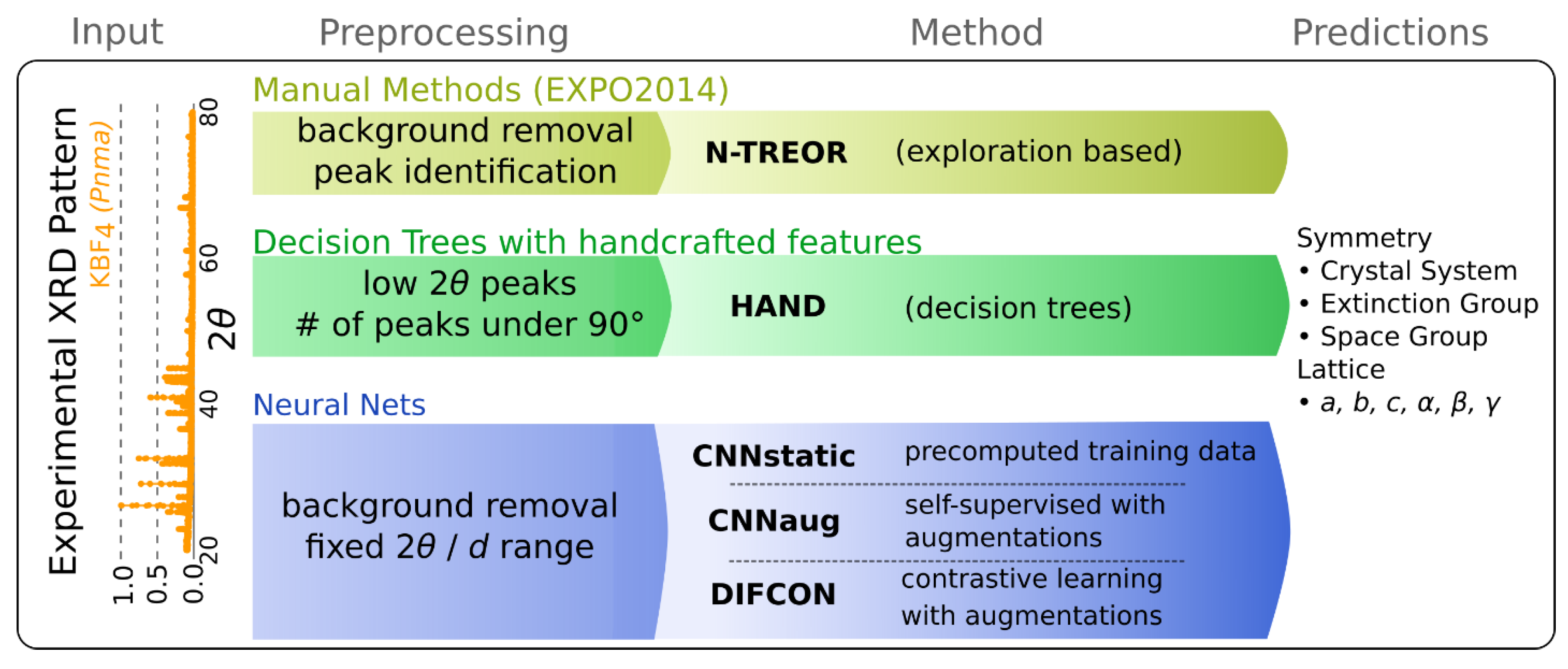
Figure 2.
Exemplary comparison of the experimental pattern of KBF4 (blue) with two randomly selected ablations (red, orange) according to the given parameters.
Figure 2.
Exemplary comparison of the experimental pattern of KBF4 (blue) with two randomly selected ablations (red, orange) according to the given parameters.
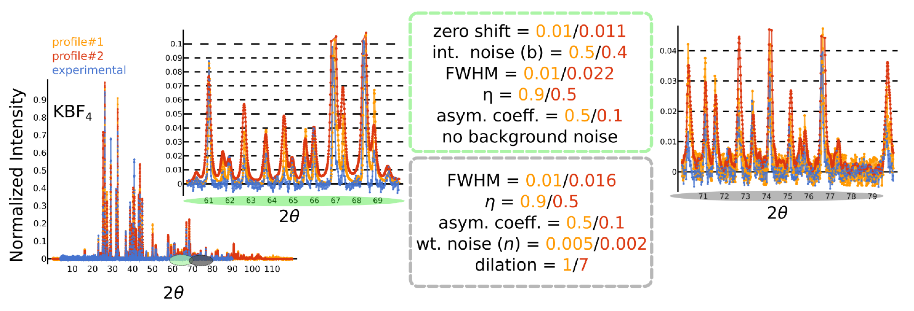
Figure 3.
Visualizing the contrastive learning framework, with positive (KBF4 vs. KBF4) and negative (KBr vs. KBF4) pairs.
Figure 3.
Visualizing the contrastive learning framework, with positive (KBF4 vs. KBF4) and negative (KBr vs. KBF4) pairs.
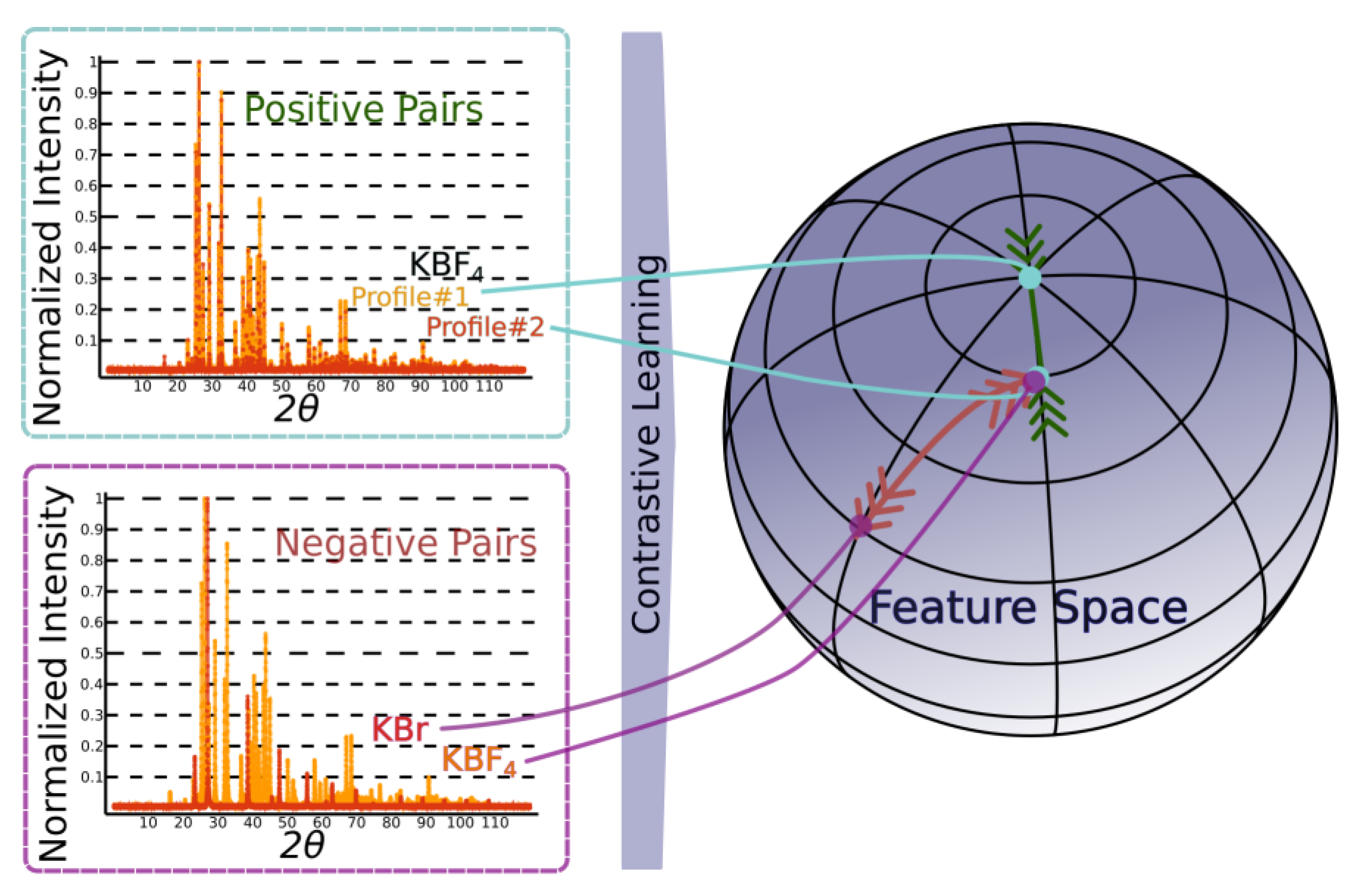
Figure 4.
The cosine similarities (color bar) of the feature representations learnt by our supervised learning model CNNstatic (left) and the SimCLR based contrastive learning model (right) for 100 randomly selected phases from a test set of phases. Each was simulated with 8 different experimental effects (like zero-shift, x & y axis noise, impurity peaks, and peak profile variation) and arranged consecutively.
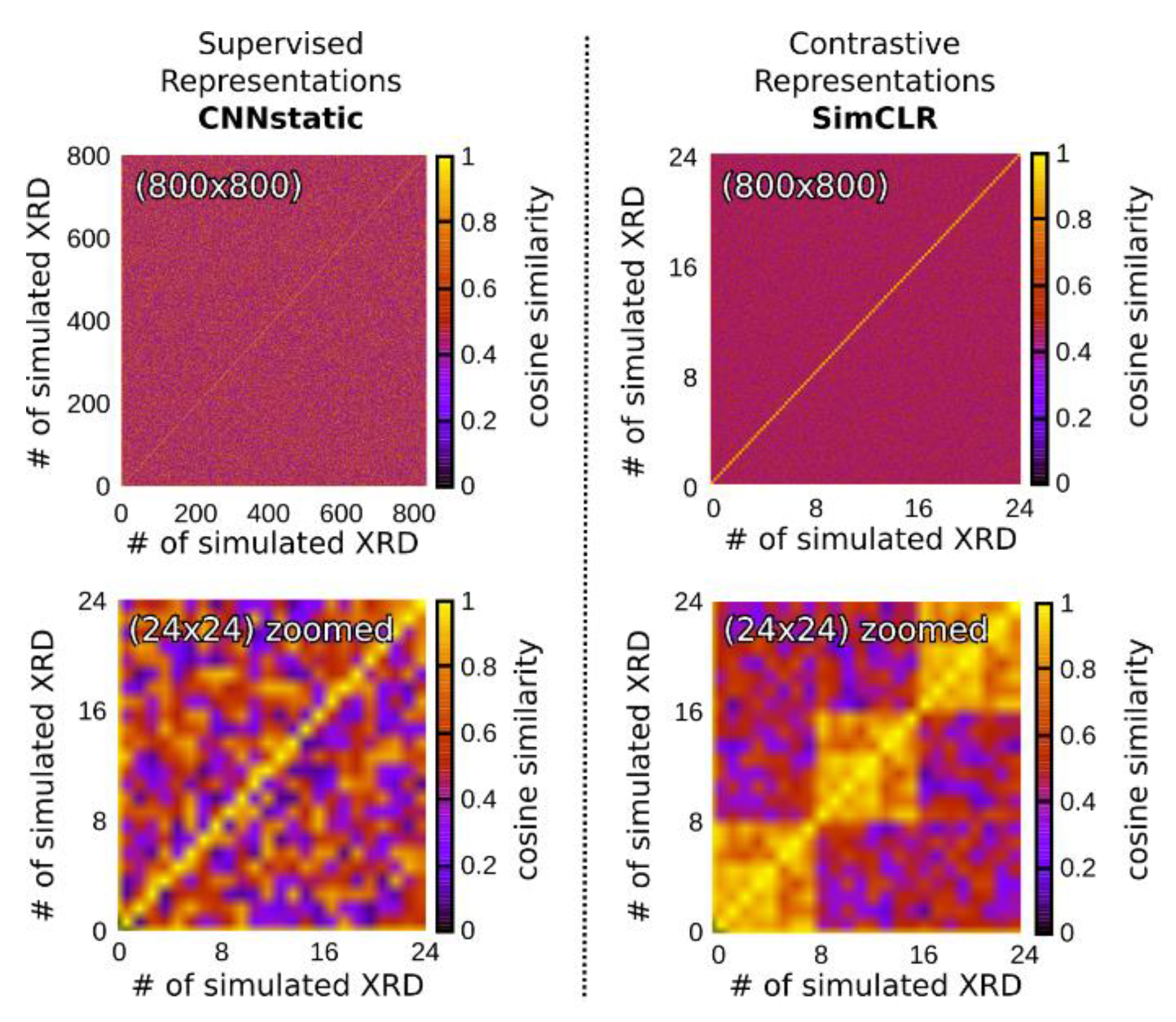

Table 1.
Overview of the signal processing operations used for simulating XRD patterns. Here signifies uniform distribution within a specific range and defines real numbers of a specific dimension. The units of the variables refer to the physical parameters and have been dropped for reasons of simplicity.
| Operation | Functional form / random variable(s) |
|---|---|
| zero shift | |
| x-axis white noise | |
| peak cropping & padding |
|
| intensity noise |
, |
| Binning (no random variables) |
, |
| impurity peaks |
|
| profile |
, |
| background noise |
|
| cropping & padding |
Disclaimer/Publisher’s Note: The statements, opinions and data contained in all publications are solely those of the individual author(s) and contributor(s) and not of MDPI and/or the editor(s). MDPI and/or the editor(s) disclaim responsibility for any injury to people or property resulting from any ideas, methods, instructions or products referred to in the content. |
© 2025 by the authors. Licensee MDPI, Basel, Switzerland. This article is an open access article distributed under the terms and conditions of the Creative Commons Attribution (CC BY) license (http://creativecommons.org/licenses/by/4.0/).
Copyright: This open access article is published under a Creative Commons CC BY 4.0 license, which permit the free download, distribution, and reuse, provided that the author and preprint are cited in any reuse.


