Commutative Geometric Algebra of Euclidean Vectors Spaces and Vector Analogues of Complex Analysis

1. Introduction

The study of scalar and vector fields in the 2$\mathbb{D}$ Euclidean vector space ${\mathbf{V}}^2$ is traditionally based on vector calculus [1], while complex analysis provides a highly structured framework for 2$\mathbb{D}$ problems [2]. An implicit connection between these areas arises from the identification of the complex plane $\mathbb{C}$ with ${\mathbb{R}}^2$, thereby allowing many results of complex analysis to be reformulated in vector form. However, the fundamental distinction between the complex plane $\mathbb{C}$ and the 2$\mathbb{D}$ Euclidean vector space ${\mathbf{V}}^2$ lies not in their geometric properties, but in their multiplicative structure. Specifically, ${\mathbf{V}}^2$ has no canonical multiplication that combines two arbitrary vectors into another vector of the same space.

In parallel, geometric (Clifford) algebra extends elementary algebra to operate on geometric objects such as vectors by introducing the geometric product of vectors in addition to vector addition. The geometric product originates from the unification of Grassmann’s exterior algebra [3] and Hamilton’s quaternion algebra [4], achieved by Clifford, giving rise to what is now known as Clifford algebra [5]. In the second half of the twentieth century, Hestenes revived and popularized the term geometric algebra [6,7]. Geometric algebra and Clifford analysis provide alternative algebraic frameworks for describing geometric quantities in higher-dimensional spaces. These approaches typically rely on non-commutative geometric products that encode both metric and orientation information.

In Clifford algebra the geometric product generates multivectors, providing a unified algebraic framework for representing geometric entities. In contrast to many traditional formalisms for manipulating geometric objects, geometric algebra also allows division by nonzero vectors. The present paper follows a different approach. Instead of extending the vector space by introducing multivectors, it defines a closed commutative geometric product directly on ${\mathbf{V}}^2$, thereby endowing the original real vector space with a new algebraic structure. More generally, this paper develops an alternative algebraic construction for scalar or vector fields in ${\mathbf{V}}^2$ , based on such a commutative geometric product. The goal is not to replace existing frameworks, but to investigate whether a commutative algebraic structure can provide a consistent foundation for vector calculus identities and their analogues in complex analysis. The construction is then extended to the 3$\mathbb{D}$ Euclidean vector space ${\mathbf{V}}^3$, where corresponding integral identities are established.

1.1. Main Contributions of the Paper

The main contributions of this paper are summarized as follows.

Commutative geometric product on${\mathbf{V}}^2$. A commutative geometric product on ${\mathbf{V}}^2$ is introduced, endowing it with an algebraic structure that is isomorphic to the algebraic structure of the field of ordered pairs of real numbers, hereafter denoted by $\mathbb{B}$ and referred to as the field of bireal numbers (also known historically as Hamilton’s couple numbers) and consequently to the complex field $\mathbb{C}$,8]. The formulation is given entirely in terms of real vectors, without introducing complex numbers as primitive objects.

Vector formulation of complex identities. Within this framework, vector analogues in ${\mathbf{V}}^2$ of classical results from complex analysis are derived, including the Cauchy integral theorem, the Cauchy integral formula, the residue theorem, and the Cauchy-Pompeiu formula. All of these results emerge naturally from the algebraic structure of ${\mathbf{V}}^2$, rather than as direct translations of their complex-analytic counterparts.

Relation to existing algebraic frameworks. The proposed vector algebra on ${\mathbf{V}}^2$ differs from other classical approaches, such as Grassmann(exterior) algebra [3] and Cliffordalgebra, which are generally non-commutative. In contrast, the present construction is based on a commutative product, leading to a different algebraic organization of vector quantities. The relationship to standard vector calculus and geometric algebra is discussed in terms of shared and distinct properties.

Extension to three-dimensional vector fields. The algebraic construction is naturally extended to the 3$\mathbb{D}$ Euclidean vector space ${\mathbf{V}}^3$. In this setting, an analogous algebraic structure is introduced, and corresponding integral identities are derived. While this extension preserves the algebraic framework, it does not claim equivalence with existing formulations such as Clifford analysis or differential forms, but rather explores a consistent generalization of the commutative approach.

1.2. Scope of the Work

The aim of this paper is not to simply replace established theories such as complex analysis, vector calculus, or Clifford analysis, but to provide an alternative commutative algebraic framework for vector fields in Euclidean spaces. The results should therefore be interpreted as structural correspondences rather than methodological substitutions.

2. Algebraic Structure of the Field of Real Vectors ${\mathbf{V}}^2$

Let ${\mathbf{V}}^2$ denote a 2$\mathbb{D}$ Euclidean vector space with orthonormal basis {$\mathbf{e},\widehat{\mathbf{e}}$}. Its elements $\mathbf{r}=x\mathbf{e}+x\widehat{\mathbf{e}}$, which are geometric vectors, form an Abelian group under vector addition.

Definition 1. 

Let ${\mathbf{V}}^2$ be equipped with two binary operations $\circ :{\mathbf{V}}^2\times {\mathbf{V}}^2\to {\mathbf{V}}^2$ and $\wedge :{\mathbf{V}}^2\times {\mathbf{V}}^2\to {\mathbf{V}}^2$ called the inner vector product and the outer vector product, respectively. The geometric vector product $★:{\mathbf{V}}^2\times {\mathbf{V}}^2\to {\mathbf{V}}^2$ is defined by

$${\mathbf{r}}_1★{\mathbf{r}}_2={\overline{\mathbf{r}}}_1\circ {\mathbf{r}}_2+{\overline{\mathbf{r}}}_1\wedge {\mathbf{r}}_2,$$

(1)

where $\overline{\mathbf{r}}=x\mathbf{e}-\widehat{x}\widehat{\mathbf{e}}$ denote the conjugate vector of a vector $\mathbf{r}=x\mathbf{e}+\widehat{x}\widehat{\mathbf{e}}\in {\mathbf{V}}^2$.

The properties of the algebraic structure (${\mathbf{V}}^2,+,★$) are determined axiomatically by the definitions of the binary operations ∘ and ∧. Accordingly, if

$${\overline{\mathbf{r}}}_1\circ {\mathbf{r}}_2=({\overline{\mathbf{r}}}_1·{\mathbf{r}}_2)\mathbf{e}\mathrm{and}{\overline{\mathbf{r}}}_1\wedge {\mathbf{r}}_2=({\overline{\mathbf{r}}}_1\times {\mathbf{r}}_2)\times \mathbf{e},$$

(2)

where ${\overline{\mathbf{r}}}_1·{\mathbf{r}}_2$ and ${\overline{\mathbf{r}}}_1\times {\mathbf{r}}_2$ are dot and cross products of vektors ${\overline{\mathbf{r}}}_1$ and ${\mathbf{r}}_2$, respectively, then it can be shown that the geometric vector product ${\mathbf{r}}_1★{\mathbf{r}}_2$, or simply ${\mathbf{r}}_1{\mathbf{r}}_2$, is commutative. Furthermore, the algebraic structure (${\mathbf{V}}^2,+,★$) is a commutative ring, whose every non-zero element $\mathbf{r}$ has a multiplicative inverse ${\mathbf{r}}^{-1}=$$\overline{\mathbf{r}}/\left(\overline{\mathbf{r}}\mathbf{r}\right)$. Therefore, ${\mathbf{V}}^2$ is a field of real vectors. Lets prove this.

Lemma 1. 

For two arbitrary vectors ${\mathbf{r}}_1=x_1\mathbf{e}+{\widehat{x}}_1\widehat{\mathbf{e}}$ and ${\mathbf{r}}_2=x_2\mathbf{e}+{\widehat{x}}_2\widehat{\mathbf{e}}$ of ${\mathbf{V}}^2$, the geometric vector product is

$${\mathbf{r}}_1{\mathbf{r}}_2={\overline{\mathbf{r}}}_1\circ {\mathbf{r}}_2+{\overline{\mathbf{r}}}_1\wedge {\mathbf{r}}_2=(x_1{x}_2-{\widehat{x}}_1{\widehat{x}}_2)\mathbf{e}+(x_1{\widehat{x}}_2+{\widehat{x}}_1{x}_2)\widehat{\mathbf{e}}.$$

(3)

Proof. 

Let ${\mathbf{r}}_1=x_1\mathbf{e}+{\widehat{x}}_1\widehat{\mathbf{e}}$ and ${\mathbf{r}}_2=x_2\mathbf{e}+{\widehat{x}}_2\widehat{\mathbf{e}}$ be two arbitrary vectors of ${\mathbf{V}}^2$. From (2)

$${\overline{\mathbf{r}}}_1\circ {\mathbf{r}}_2=({\overline{\mathbf{r}}}_1·{\mathbf{r}}_2)\mathbf{e}=(x_1{x}_2-{\widehat{x}}_1{\widehat{x}}_2)\mathbf{e}\mathrm{and}$$

$${\overline{\mathbf{r}}}_1\wedge {\mathbf{r}}_2=({\overline{\mathbf{r}}}_1\times {\mathbf{r}}_2)\times \mathbf{e}=(x_1{\widehat{x}}_2+{\widehat{x}}_1{x}_2)\widehat{\mathbf{e}}.$$

Hence

$${\mathbf{r}}_1{\mathbf{r}}_2={\overline{\mathbf{r}}}_1\circ {\mathbf{r}}_2+{\overline{\mathbf{r}}}_1\wedge {\mathbf{r}}_2=(x_1{x}_2-{\widehat{x}}_1{\widehat{x}}_2)\mathbf{e}+(x_1{\widehat{x}}_2+{\widehat{x}}_1{x}_2)\widehat{\mathbf{e}}.$$

□

Theorem 1. 

The algebraic structure $({\mathbf{V}}^2,+,★)$ satisfies all field axioms. Hence, it is a field.

Proof. Commutativity: By Lemma 1,

$${\mathbf{r}}_2{\mathbf{r}}_1={\overline{\mathbf{r}}}_2\circ {\mathbf{r}}_1+{\overline{\mathbf{r}}}_2\wedge {\mathbf{r}}_1=({\overline{\mathbf{r}}}_2·{\mathbf{r}}_1)\mathbf{e}+({\overline{\mathbf{r}}}_2\times {\mathbf{r}}_1)\times \mathbf{e}=$$

$$=(x_2{x}_1-{\widehat{x}}_2{\widehat{x}}_1)\mathbf{e}+(x_2{\widehat{x}}_1+{\widehat{x}}_2{x}_1)\widehat{\mathbf{e}}={\mathbf{r}}_1{\mathbf{r}}_2.$$

Associativity: Using Lemma 1, $\left({\mathbf{r}}_1{\mathbf{r}}_2\right){\mathbf{r}}_3$ equals

$$[(x_1{x}_2-{\widehat{x}}_1{\widehat{x}}_2)\mathbf{e}+(x_1{\widehat{x}}_2+{\widehat{x}}_1{x}_2)\widehat{\mathbf{e}}](x_3\mathbf{e}+{\widehat{x}}_3\widehat{\mathbf{e}})=$$

$$=[(x_1{x}_2-{\widehat{x}}_1{\widehat{x}}_2)x_3-(x_1{\widehat{x}}_2+{\widehat{x}}_1{x}_2){\widehat{x}}_3]\mathbf{e}+[(x_1{x}_2-{\widehat{x}}_1{\widehat{x}}_2){\widehat{x}}_3+(x_1{\widehat{x}}_2+{\widehat{x}}_1{x}_2)x_3]\widehat{\mathbf{e}}.$$

After expanding and rearranging terms, it equals

$$[(x_1{x}_2{x}_3-{\widehat{x}}_1{\widehat{x}}_2{x}_3-x_1{\widehat{x}}_2{\widehat{x}}_3-{\widehat{x}}_1{x}_2{\widehat{x}}_3)\mathbf{e}+(x_1{x}_2{\widehat{x}}_3-{\widehat{x}}_1{\widehat{x}}_2{\widehat{x}}_3+x_1{\widehat{x}}_2{x}_3-{\widehat{x}}_1{x}_2{x}_3)\widehat{\mathbf{e}}.$$

The same expression is obtained for ${\mathbf{r}}_1\left({\mathbf{r}}_2{\mathbf{r}}_3\right)$, therefore $\left({\mathbf{r}}_1{\mathbf{r}}_2\right){\mathbf{r}}_3={\mathbf{r}}_1\left({\mathbf{r}}_2{\mathbf{r}}_3\right)$.

Distributivity: Directly from Lemma 1, $({\mathbf{r}}_1+{\mathbf{r}}_2){\mathbf{r}}_3={\mathbf{r}}_1{\mathbf{r}}_3+{\mathbf{r}}_2{\mathbf{r}}_3$ and similarly ${\mathbf{r}}_1({\mathbf{r}}_2+{\mathbf{r}}_3)={\mathbf{r}}_1{\mathbf{r}}_2+{\mathbf{r}}_1{\mathbf{r}}_3$.

Multiplicative identity: Since $\mathbf{ee}=\mathbf{e}$ and $\mathbf{e}\widehat{\mathbf{e}}=\widehat{\mathbf{e}}$, it follows that $\mathbf{er}=\mathbf{re}=\mathbf{r}$. Therefore, $\mathbf{e}$ is the multiplicative identity.

Inverse: As $\mathbf{r}\overline{\mathbf{r}}=(x^2+{\widehat{x}}^2)\mathbf{e}$, every nonzero vector has inverse ${\mathbf{r}}^{-1}=\overline{\mathbf{r}}/(x^2+{\widehat{x}}^2)$. Indeed, ${\mathbf{rr}}^{-1}=\mathbf{e}$. □

Remark 1. 

Although the algebraic structure $({\mathbf{V}}^2,+,★)$ is constructed from the newly defined geometric product of vectors $\left(\right)$, it is not a new field in the algebraic sense. It is naturally isomorphic to the field $\mathbb{B}$, and this isomorphism is given by $\Phi (x\mathbf{e}+\widehat{x}\widehat{\mathbf{e}})=(x,\widehat{x})$. The field $\mathbb{B}$ is naturally isomorphic to the field of complex numbers $\mathbb{C}$ via the mapping $\Psi \left((x,\widehat{x})\right)=(x,i\widehat{x})$. Consequently, ${\mathbf{V}}^2\cong \mathbb{B}\cong \mathbb{C}$. The novelty of the present paper lies not in the underlying algebraic field itself, but in the introduction of a commutative geometric product on the Euclidean vector space ${\mathbf{V}}^2$ that realizes an algebraic field structure intrinsically in terms of vectors.

Division by a nonzero vector in ${\mathbf{V}}^2$, based on the inverse element ${\mathbf{r}}^{-1}=\overline{\mathbf{r}}/∥\mathbf{r}∥$, where $∥\mathbf{r}∥=r=\left|\sqrt[2]{\left|\overline{\mathbf{r}}\mathbf{r}\right|}\right|=\left|\sqrt[2]{x^2+{\widehat{y}}^2}\right|$, is one of the fundamental consequences of introducing the commutative geometric product of vectors in ${\mathbf{V}}^2$. The geometric quotient follows directly from the product defined by (3). Hence, if ${\mathbf{r}}_0$ is the unit vector associated with the position vector $\mathbf{r}$ $(\mathbf{r}=$ $r{\mathbf{r}}_0)$ in ${\mathbf{V}}^2$, then ${\mathbf{r}}_0^{-1}={\overline{\mathbf{r}}}_0$ and

$${\displaystyle \frac{{\mathbf{r}}_{0_1}}{{\mathbf{r}}_{0_2}}}={\mathbf{r}}_{0_1}{\overline{\mathbf{r}}}_{0_2}={\overline{\mathbf{r}}}_{0_1}\circ {\overline{\mathbf{r}}}_{0_2}+{\overline{\mathbf{r}}}_{0_1}\wedge {\overline{\mathbf{r}}}_{0_2}={\mathbf{r}}_{0_1}\circ {\mathbf{r}}_{0_2}-{\mathbf{r}}_{0_1}\wedge {\mathbf{r}}_{0_2}.$$

(4)

Here,

$${\mathbf{r}}_{0_1}\circ {\mathbf{r}}_{0_2}={\displaystyle \frac{1}{2}}({\displaystyle \frac{{\mathbf{r}}_{0_2}}{{\mathbf{r}}_{0_1}}}+{\displaystyle \frac{{\mathbf{r}}_{0_1}}{{\mathbf{r}}_{0_2}}})\mathrm{and}{\mathbf{r}}_{0_1}\wedge {\mathbf{r}}_{0_2}={\displaystyle \frac{1}{2}}({\displaystyle \frac{{\mathbf{r}}_{0_2}}{{\mathbf{r}}_{0_1}}}-{\displaystyle \frac{{\mathbf{r}}_{0_1}}{{\mathbf{r}}_{0_2}}}),$$

(5)

where ${\mathbf{r}}_{0_1}\circ {\mathbf{r}}_{0_2}=({\mathbf{r}}_{0_1}·{\mathbf{r}}_{0_2})\mathbf{e}$ and ${\mathbf{r}}_{0_1}\wedge {\mathbf{r}}_{0_2}=({\mathbf{r}}_{0_1}\times {\mathbf{r}}_{0_2})\times \mathbf{e}$ are the symmetric and antisymmetric parts of the geometric product ${\overline{\mathbf{r}}}_{0_1}{\mathbf{r}}_{0_2}$, respectively. Since the geometric product of two vectors is a vector in ${\mathbf{V}}^2$, it follows that $\mathbf{re}=(\overline{\mathbf{r}}·\mathbf{e})\mathbf{e}+(\overline{\mathbf{r}}\times \mathbf{e})\times \mathbf{e}=x\mathbf{e}+y\widehat{\mathbf{e}}=\mathbf{r}$ and $\mathbf{r}\widehat{\mathbf{e}}=(\overline{\mathbf{r}}·\widehat{\mathbf{e}})\mathbf{e}+(\overline{\mathbf{r}}\times \widehat{\mathbf{e}})\times \mathbf{e}={\mathbf{r}}_{\perp }$. The vector ${\mathbf{r}}_{\perp }$ is orthogonal to the vector $\mathbf{r}$, that is, ${\mathbf{r}}_{\perp }$ is the vector obtained by rotating the vector $\mathbf{r}=r{\mathbf{r}}_0=r(\mathbf{e}cos\phi +\widehat{\mathbf{e}}sin\phi )$, where $\phi$ is the angle between the vector $\mathbf{r}$ and the vector $\mathbf{e}$, by $\pi /2$ radians in the positive mathematical direction. Furthermore, the unit vector ${\overline{\mathbf{r}}}_0=cos\phi \mathbf{e}-sin\phi \widehat{\mathbf{e}}$ is the inverse vector ${\mathbf{r}}_0^{-1}$. Consequently, ${\overline{\mathbf{r}}}_0$ is also the unit vector associated with the inverse vector ${\mathbf{r}}^{-1}$, so that ${\mathbf{r}}^{-1}={\overline{\mathbf{r}}}_0/r$ and $\overline{\mathbf{r}}=r{\overline{\mathbf{r}}}_0$.

Let c$\widehat{\mathbf{e}}$s· denote the operator $\mathbf{e}cos·+\widehat{\mathbf{e}}sin·$. Accordingly, c$\widehat{\mathbf{e}}$s·c$\widehat{\mathbf{e}}$s·=c$\widehat{\mathbf{e}}$s$(·+·)$, (c$\widehat{\mathbf{e}}$s${·)}^{-1}=$c$\widehat{\mathbf{e}}$s$(-·)$ and d(c$\widehat{\mathbf{e}}$s$·)=\widehat{\mathbf{e}}$c$\widehat{\mathbf{e}}$s·d·. Therefore, the operator c$\widehat{\mathbf{e}}$s· satisfies the some fundamental properties of the exponential function. Consequently, we write c$\widehat{\mathbf{e}}$s$·=exp(\widehat{\mathbf{e}}·)$. So, ${\mathbf{r}}_0$= c$\widehat{\mathbf{e}}$s$\phi =exp\left(\widehat{\mathbf{e}}\phi \right)$. By analogy with complex analysis, we introduce the vector logarithmic function

$$log\mathbf{r}=lnr\mathbf{e}+\phi \widehat{\mathbf{e}},$$

(6)

where $2\phi \widehat{\mathbf{e}}=2log{\mathbf{r}}_0=log({\mathbf{r}}_0/{\overline{\mathbf{r}}}_0)$. Furthermore, Log$\mathbf{r}$$=lnr\mathbf{e}+(\phi +2\pi n)\widehat{\mathbf{e}}$, $n\in \mathbb{Z}$.

Let ${\widehat{\mathbf{r}}}_0=-{\mathbf{r}}_{0\perp }^{-1}=\mathbf{e}sin\phi +\widehat{\mathbf{e}}cos\phi =$s$\widehat{\mathbf{e}}$c$\phi =\widehat{\mathbf{e}}{\overline{\mathbf{r}}}_0$. The ordered pair $({\overline{\mathbf{r}}}_0,{\widehat{\mathbf{r}}}_0)$ forms the inverse orthonormal basis corresponding to the orthonormal basis $({\mathbf{r}}_0,{\mathbf{r}}_{0\perp })$ of ${\mathbf{V}}_2$. For an arbitrary vector $\varrho \in {\mathbf{V}}_2$, multiplication by the basis vectors has a simple geometric interpretation. The products $\varrho {\mathbf{r}}_0$ and $\varrho {\mathbf{r}}_{0\perp }$ rotate the vector $\varrho$ through the angles $\phi$ and $\pi /2+\phi$, respectively, in the positive mathematical direction. Likewise, multiplication by the inverse basis vectors ${\overline{\mathbf{r}}}_0$ and ${\widehat{\mathbf{r}}}_0$, rotates $\varrho$ through the angles $-\phi$ and $\pi /2-\phi$, respectively, in the positive mathematical direction.

On the basis of the geometric products $\mathbf{ee}=\mathbf{e}$, $\mathbf{e}\widehat{\mathbf{e}}=\widehat{\mathbf{e}}$ and $\widehat{\mathbf{e}}\widehat{\mathbf{e}}=-\mathbf{e}$, together with

$${\mathbf{r}}_0{\mathbf{r}}_0=({\overline{\mathbf{r}}}_0·{\mathbf{r}}_0)\mathbf{e}+({\overline{\mathbf{r}}}_0\times {\mathbf{r}}_0)\times \mathbf{e}=({cos}^2\phi -{sin}^2\phi )\mathbf{e}+2(cos\phi sin\phi )\widehat{\mathbf{e}},$$

(7)

${\mathbf{r}}_0{\overline{\mathbf{r}}}_0=\mathbf{e}$ and ${\mathbf{r}}_0{\widehat{\mathbf{r}}}_0=\widehat{\mathbf{e}}$ ($\widehat{\mathbf{r}}=\overline{\mathbf{r}}\widehat{\mathbf{e}}$), all remaining geometric products between the basis vectors ${\mathbf{r}}_0$, ${\mathbf{r}}_{0\perp }$, ${\overline{\mathbf{r}}}_0$ and ${\widehat{\mathbf{r}}}_0$ follow directly from these identities.

2.1. Differential Operators in the Field ${\mathbf{V}}^2$

Let define the differential operator $d=dr{\partial }_r+d\phi {\partial }_{\phi }$. According to that $d\mathbf{r}=dr{\mathbf{r}}_0+d\phi {\mathbf{r}}_{\perp }$, $d{\mathbf{r}}_{\perp }=\widehat{\mathbf{e}}d\mathbf{r}=dr{\mathbf{r}}_{0\perp }-d\phi \mathbf{r}$ and $d\widehat{\mathbf{r}}=\widehat{\mathbf{e}}d\overline{\mathbf{r}}=\widehat{\mathbf{e}}(dr{\overline{\mathbf{r}}}_0-d\phi \widehat{\mathbf{r}})=dr{\widehat{\mathbf{r}}}_0+d\phi \overline{\mathbf{r}}$. Motivated by the identities $2rcos\phi \mathbf{e}=\mathbf{r}+\overline{\mathbf{r}}$ and $2rsin\phi \widehat{\mathbf{e}}=\mathbf{r}-\overline{\mathbf{r}}$, we define the vector differential operators, which are vector analogues of the Wirtinger operators [9],

$${ð}_{\mathbf{r}}={\partial }_{\mathbf{r}}r{\partial }_r+{\partial }_{\mathbf{r}}\phi {\partial }_{\phi }={\displaystyle \frac{1}{2}}({\overline{\mathbf{r}}}_0{\partial }_r-{\displaystyle \frac{{\widehat{\mathbf{r}}}_0}{r}}{\partial }_{\phi })\mathrm{and}{ð}_{\overline{\mathbf{r}}}={\overline{ð}}_{\mathbf{r}}={\displaystyle \frac{1}{2}}({\mathbf{r}}_0{\partial }_r+{\displaystyle \frac{{\mathbf{r}}_{0\perp }}{r}}{\partial }_{\phi }),$$

(8)

where

$${\partial }_{\mathbf{r}}r={\displaystyle \frac{1}{2r}}{\partial }_{\mathbf{r}}\left(r^2\right)={\displaystyle \frac{{\overline{\mathbf{r}}}_0}{2}}\mathrm{and}{\partial }_{\mathbf{r}}\phi ={cos}^2\phi {\partial }_{\mathbf{r}}tan\phi ={\left({\displaystyle \frac{\mathbf{r}+\overline{\mathbf{r}}}{2r}}\right)}^2{\displaystyle \frac{-2\widehat{\mathbf{e}}\overline{\mathbf{r}}}{{(\mathbf{r}+\overline{\mathbf{r}})}^2}}=-{\displaystyle \frac{{\widehat{\mathbf{r}}}_0}{2r}}.$$

(9)

Remark 2. 

It is important to emphasize that the differentiation rules for geometric products and geometric quotients are identical to those for ordinary products and quotients. In particular, $d\left(\mathbf{r}/\overline{\mathbf{r}}\right)=\left(\overline{\mathbf{r}}d\mathbf{r}-\mathbf{r}d\overline{\mathbf{r}}\right)/{\overline{\mathbf{r}}}^2$. Indeed,

$$d{\displaystyle \frac{\mathbf{r}}{\overline{\mathbf{r}}}}=\left(d{\displaystyle \frac{1}{r^2}}\right){\mathbf{r}}^2+{\displaystyle \frac{1}{r^2}}d{\mathbf{r}}^2=-2({\displaystyle \frac{{\mathbf{r}}^2}{r^3}}dr-{\displaystyle \frac{1}{r^2}}\mathbf{r}d\mathbf{r})=$$

(10)

$$=-2[{\displaystyle \frac{{\mathbf{r}}^2}{2r^4}}(\overline{\mathbf{r}}d\mathbf{r}+\mathbf{r}d\overline{\mathbf{r}})-{\displaystyle \frac{1}{r^2}}\mathbf{r}d\mathbf{r}]=-2[{\displaystyle \frac{1}{2{\overline{\mathbf{r}}}^2}}(\overline{\mathbf{r}}d\mathbf{r}+\mathbf{r}d\overline{\mathbf{r}})-{\displaystyle \frac{1}{{\overline{\mathbf{r}}}^2}}\overline{\mathbf{r}}d\mathbf{r}]={\displaystyle \frac{\overline{\mathbf{r}}d\mathbf{r}-\mathbf{r}d\overline{\mathbf{r}}}{{\overline{\mathbf{r}}}^2}}.$$

It follows immediately that $2{ð}_{\overline{\mathbf{r}}}$ is the gradient operator. Similarly, the symmetric part of the geometric product $2{ð}_{\mathbf{r}}\mathbf{F}$ is the vector representation of the divergence (div) of the vector field $\mathbf{F}=F{\mathbf{r}}_0+F_{\perp }{\mathbf{r}}_{0\perp }$, whereas the antisymmetric part is the vector representation of the curl, since

$$2{ð}_{\mathbf{r}}\mathbf{F}={\displaystyle \frac{{\overline{\mathbf{r}}}_0{\mathbf{r}}_0}{r}}[{\partial }_r\left(rF\right)+{\partial }_{\phi }{F}_{\perp }]+{\displaystyle \frac{{\overline{\mathbf{r}}}_0{\mathbf{r}}_{0\perp }}{r}}[{\partial }_r\left(r{F}_{\perp }\right)-{\partial }_{\phi }F]=$$

(11)

$$={\overline{\mathbf{r}}}_0{\mathbf{r}}_{0}div\mathbf{F}+curl\mathbf{F}\times {\overline{\mathbf{r}}}_0{\mathbf{r}}_0.$$

On the other hand,

$${\overline{\mathbf{r}}}_0{ð}_{\overline{\mathbf{r}}}\circ {\overline{\mathbf{r}}}_0\mathbf{F}+{\overline{\mathbf{r}}}_0{ð}_{\overline{\mathbf{r}}}\wedge {\overline{\mathbf{r}}}_0\mathbf{F}={\mathbf{r}}_0{ð}_{\mathbf{r}}\left({\overline{\mathbf{r}}}_0\mathbf{F}\right)=-{\displaystyle \frac{{\overline{\mathbf{r}}}_0}{2r}}\mathbf{F}+{ð}_{\mathbf{r}}\mathbf{F}.$$

(12)

Consequently,

$$2{ð}_{\mathbf{r}}\mathbf{F}={\displaystyle \frac{2}{r^2}}[(\overline{\mathbf{r}}{ð}_{\overline{\mathbf{r}}}\circ \overline{\mathbf{r}}\mathbf{F})+(\overline{\mathbf{r}}{ð}_{\overline{\mathbf{r}}}\wedge \overline{\mathbf{r}}\mathbf{F})].$$

(13)

Hence, $div\mathbf{F}=2(\overline{\mathbf{r}}{ð}_{\overline{\mathbf{r}}}·\overline{\mathbf{r}}\mathbf{F})/r^2$ and $curl\mathbf{F}=2(\overline{\mathbf{r}}{ð}_{\overline{\mathbf{r}}}\times \overline{\mathbf{r}}\mathbf{F})/r^2$.

Similarly,

$${\mathbf{r}}_0{ð}_{\mathbf{r}}\circ {\overline{\mathbf{r}}}_0\mathbf{F}+{\mathbf{r}}_0{ð}_{\mathbf{r}}\wedge {\overline{\mathbf{r}}}_0\mathbf{F}={\overline{\mathbf{r}}}_0{ð}_{\overline{\mathbf{r}}}\left({\overline{\mathbf{r}}}_0\mathbf{F}\right)={\overline{\mathbf{r}}}_0({\displaystyle \frac{1}{2r}}\mathbf{F}+{\overline{\mathbf{r}}}_0{ð}_{\overline{\mathbf{r}}}\mathbf{F})\mathrm{and}$$

(14)

$$2{ð}_{\overline{\mathbf{r}}}\mathbf{F}={\displaystyle \frac{{\mathbf{r}}_0}{r}}[{\mathbf{r}}_0(r{\partial }_{r}F-{\partial }_{\phi }{F}_{\perp })+{\mathbf{r}}_{0\perp }(r{\partial }_r{F}_{\perp }+{\partial }_{\phi }F)-\mathbf{F}]=grad\mathbf{F}.$$

(15)

Definition 2. 

The operator $d\mathbf{r}{ð}_{\mathbf{r}}$ is called the $1\mathbb{D}$ differential-form operator.

The vector operator

$$\mathbf{d}={\mathbf{r}}_0(d\mathbf{r}{ð}_{\mathbf{r}}+d\overline{\mathbf{r}}{ð}_{\overline{\mathbf{r}}})=2{\mathbf{r}}_0(d\mathbf{r}\circ {ð}_{\overline{\mathbf{r}}})={\mathbf{r}}_0(dr{\partial }_r+d\phi {\partial }_{\phi })={\mathbf{r}}_{0}d,$$

(16)

is called the radial vector differential operator. The vector operator

$${\mathbf{d}}_{\perp }={\mathbf{r}}_0(d\mathbf{r}{ð}_{\mathbf{r}}-d\overline{\mathbf{r}}{ð}_{\overline{\mathbf{r}}})=-2{\mathbf{r}}_0(d\mathbf{r}\wedge {ð}_{\overline{\mathbf{r}}})={\mathbf{r}}_{0\perp }(rd\phi {\partial }_r-{\displaystyle \frac{1}{r}}dr{\partial }_{\phi })={\mathbf{r}}_{0\perp }\widehat{d}$$

(17)

is called the transverse vector differential operator. Accordingly,

$$\mathbf{d}\phi ={\mathbf{r}}_0({ð}_{\mathbf{r}}\phi d\mathbf{r}+{ð}_{\overline{\mathbf{r}}}\phi d\overline{\mathbf{r}})={\mathbf{r}}_{0}d\phi =-{\displaystyle \frac{{\mathbf{r}}_{0\perp }}{2}}dlog\left({\displaystyle \frac{\mathbf{r}}{\overline{\mathbf{r}}}}\right)\mathrm{and}$$

(18)

$$\mathbf{d}r={\mathbf{r}}_0\left({ð}_{\mathbf{r}}rd\mathbf{r}+{ð}_{\overline{\mathbf{r}}}rd\overline{\mathbf{r}}\right)={\mathbf{r}}_{0}dr={\mathbf{r}}_{0}d{\left(\mathbf{r}\overline{\mathbf{r}}\right)}^{{\displaystyle \frac{1}{2}}}={\displaystyle \frac{\mathbf{r}}{2}}dlog\left(\mathbf{r}\overline{\mathbf{r}}\right),$$

(19)

since $\mathbf{r}=r$c$\widehat{\mathbf{e}}$s$\phi =rexp\left(\phi \widehat{\mathbf{e}}\right)$ and $2\phi \widehat{\mathbf{e}}=$$log(\mathbf{r}/\overline{\mathbf{r}})$. Therefore,

$${\widehat{\mathbf{r}}}_0\mathbf{d}r\mathbf{d}\phi ={\mathbf{r}}_{0\perp }drd\phi ={\displaystyle \frac{\mathbf{r}}{4}}dlog\left(\mathbf{r}\overline{\mathbf{r}}\right)dlog\left({\displaystyle \frac{\mathbf{r}}{\overline{\mathbf{r}}}}\right).$$

(20)

Moreover,

$${\displaystyle \frac{\mathbf{r}}{4}}dlog\left(\mathbf{r}\overline{\mathbf{r}}\right)dlog\left({\displaystyle \frac{\mathbf{r}}{\overline{\mathbf{r}}}}\right)={\displaystyle \frac{\mathbf{r}}{4r^4}}(\overline{\mathbf{r}}d\mathbf{r}+\mathbf{r}d\overline{\mathbf{r}})(\overline{\mathbf{r}}d\mathbf{r}-\mathbf{r}d\overline{\mathbf{r}})={\displaystyle \frac{\mathbf{r}}{4r^2}}[{\left({\overline{\mathbf{r}}}_{0}d\mathbf{r}\right)}^2-{\left({\mathbf{r}}_{0}d\overline{\mathbf{r}}\right)}^2].$$

(21)

Using the above identities,

$${\displaystyle \frac{{\mathbf{r}}_0}{2}}(\mathbf{d}\overline{\mathbf{r}}\wedge \overline{\mathbf{d}}\mathbf{r})={\displaystyle \frac{{\mathbf{r}}_0}{4}}(\overline{\mathbf{d}}\mathbf{r}\overline{\mathbf{d}}\mathbf{r}-\mathbf{d}\overline{\mathbf{r}}\mathbf{d}\overline{\mathbf{r}})=\widehat{\mathbf{r}}\mathbf{d}r\mathbf{d}\phi ={\mathbf{r}}_{\perp }drd\phi ,$$

(22)

since $\overline{\mathbf{d}\overline{\mathbf{r}}}={\overline{\mathbf{r}}}_{0}d\mathbf{r}=\overline{\mathbf{d}}\mathbf{r}$. The above vector identity can also be derived directly by introducing the Jacobian determinant of the bijective mapping ${\mathbf{V}}^2\to {\mathbf{V}}^2$, defined by the system of vector equations $2lnr\mathbf{e}=log\left(\mathbf{r}\overline{\mathbf{r}}\right)$ and $2\phi \widehat{\mathbf{e}}=$$log(\mathbf{r}/\overline{\mathbf{r}})$, as follows

$$\mathbf{J}=\left|\begin{array}{cc}{\partial }_{r}log\left(\mathbf{r}\overline{\mathbf{r}}\right)& {\partial }_{\phi }log\left(\mathbf{r}\overline{\mathbf{r}}\right)\\ {\partial }_{r}log(\mathbf{r}/\overline{\mathbf{r}})& {\partial }_{\phi }log(\mathbf{r}/\overline{\mathbf{r}})\end{array}\right|=\left|\begin{array}{cc}2r^{-1}\mathbf{e}& \mathbf{0}\\ \mathbf{0}& 2\widehat{\mathbf{e}}\end{array}\right|={\displaystyle \frac{4}{r}}\widehat{\mathbf{e}}.$$

(23)

In this case, $4{\mathbf{r}}_{0\perp }drd\phi =\mathbf{rJ}drd\phi =\mathbf{r}dlog\left(\mathbf{r}\overline{\mathbf{r}}\right)dlog(\mathbf{r}/\overline{\mathbf{r}})$, which leads to (20). The vector $d\mathbf{S}=(\mathbf{d}\overline{\mathbf{r}}\wedge \overline{\mathbf{d}}\mathbf{r})/2=rdrd\phi {\mathbf{r}}_{0\perp }{\overline{\mathbf{r}}}_0=dS\widehat{\mathbf{e}}$ represents the Lebesgue measure of an infinitesimal surface element in ${\mathbf{V}}_2$.

Definition 3. 

Let ${ð}_{\mathbf{r}\overline{\mathbf{r}}}^2={ð}_{\overline{\mathbf{r}}}{ð}_{\mathbf{r}}$ and $d\mathbf{S}=(\mathbf{d}\overline{\mathbf{r}}\wedge \overline{\mathbf{d}}\mathbf{r})/2$. The geometric product $d\mathbf{S}{ð}_{\mathbf{r}\overline{\mathbf{r}}}^2$ is called the $2\mathbb{D}$ differential-form operator.

2.2. The Fundamental Theorem of Integral Calculus in ${\mathbf{V}}_2$

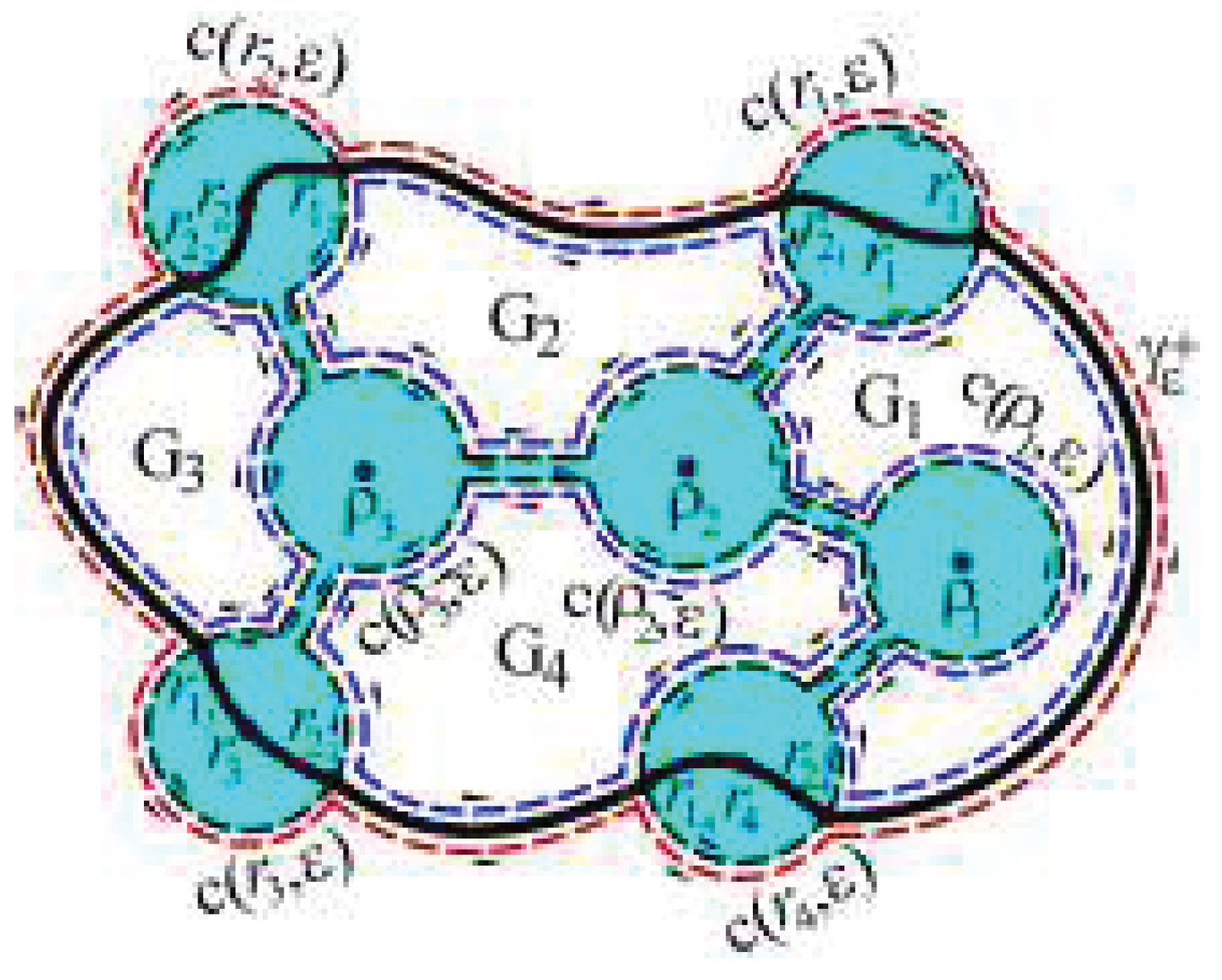
Let $\gamma$ be a closed smooth Jordan curve forming the boundary $\partial G$ of an arbitrary region G in ${\mathbf{V}}_2$. Let ${\mathbf{r}}_i$ ($i=1,2,...,n_{\gamma }$) be isolated points on $\gamma$, each surrounded by circles $c({\mathbf{r}}_i,\epsilon )$ of arbitrarily small radius $\epsilon$. Each circle intersect $\gamma$ at two points, denoted by ${\mathbf{r}}_{1_i}$ and ${\mathbf{r}}_{2_i}$, and the circles are pairwise disjoint. Let ${\varrho }_j$ ($j=1,2,...,n_G$) be isolated points in G , each surrounded by circles $c({\varrho }_j,\epsilon )$, where the circles are also pairwise disjoint. A simply connected region ${\mathcal{R}}_{\epsilon }$, containing all points ${\mathbf{r}}_i$ and ${\varrho }_j$, is constructed by connecting the circles $c({\varrho }_j,\epsilon )$, successively with pairs of parallel line segments $l_{j_1}$ and $l_{j_2}$, separated by a distance ${\delta }_j\ll \epsilon$. Likewise, each circle $c({\mathbf{r}}_i,\epsilon )$ is connected to a unique circle $c({\varrho }_j,\epsilon )$ by a pair of parallel line segments $l_{i_1}$ and $l_{i_2}$, separated by a distance ${\delta }_i\ll \epsilon$. The boundary $\partial {\mathcal{R}}_{\epsilon }$ of ${\mathcal{R}}_{\epsilon }$ (blue region in Figure 1), lies inside G and divides the region G into $n_{\gamma }$ subregions $G_i$.

Accordingly, we define the vector integral operator along $\gamma$ by

$$vt{\int }_{{\gamma }^{+}}^{⥀}{\overline{\mathbf{r}}}_0(\mathbf{d}+{\mathbf{d}}_{\perp })=2vt{\int }_{{\gamma }^{+}}^{⥀}d\mathbf{r}{ð}_{\mathbf{r}}=vt{\int }_{{\gamma }^{+}}^{⥀}[(d\mathbf{r}\circ grad)-(d\mathbf{r}\wedge grad)],$$

(24)

where $vt$ denotes the total value of an improper integral [10,11,12,13,14,15], defined by

$$vt{\int }_{{\gamma }^{+}}^{⥀}d\mathbf{r}{ð}_{\mathbf{r}}=\underset{\epsilon \to 0^{+}}{lim}{\int }_{{\gamma }_{\epsilon }^{+}}^{⥀}d\mathbf{r}{ð}_{\mathbf{r}}=\underset{\epsilon \to 0^{+}}{lim}({\int }_{\partial {\mathcal{R}}_{\epsilon }}^{⥀}d\mathbf{r}{ð}_{\mathbf{r}}+{\displaystyle \sum _{i=1}^{n_{\gamma }}}{\int }_{\partial G_i}^{⥀}d\mathbf{r}{ð}_{\mathbf{r}})=$$

(25)

$$=vp{\int }_{\gamma }^{⥀}d\mathbf{r}{ð}_{\mathbf{r}}+\underset{\epsilon \to 0^{+}}{lim}{\displaystyle \sum _{i=1}^{n_{\gamma }}}{\int }_{\partial c({\mathbf{r}}_i,\epsilon )}^{\stackrel{⤺}{{\mathbf{r}}_{2_i}{\mathbf{r}}_{1_i}}}d\mathbf{r}{ð}_{\mathbf{r}}=vt{\int }_{{\gamma }^{-}}^{⥀}d\mathbf{r}{ð}_{\mathbf{r}}+\underset{\epsilon \to 0^{+}}{lim}{\displaystyle \sum _{i=1}^{n_{\gamma }}}{\int }_{\partial c({\mathbf{r}}_i,\epsilon )}^{⥀}d\mathbf{r}{ð}_{\mathbf{r}},$$

Here, $vp$ denotes the Cauchy principal value. The vector integral operator

$$\underset{\epsilon \to 0^{+}}{lim}{\int }_{\partial {\mathcal{R}}_{\epsilon }}^{⥀}d\mathbf{r}{ð}_{\mathbf{r}}=2\pi \widehat{\mathbf{e}}{\displaystyle \sum _{i=1}^{n_{\gamma }}}Res\left({ð}_{\mathbf{r}},{\mathbf{r}}_i\right)+{\displaystyle \sum _{i=1}^{n_{\gamma }}}({\int }_{l_i^{+}}d\mathbf{r}{ð}_{\mathbf{r}}-{\int }_{l_i^{-}}d\mathbf{r}{ð}_{\mathbf{r}})+$$

(26)

$$+2\pi \widehat{\mathbf{e}}{\displaystyle \sum _{j=1}^{n_G}}Res({ð}_{\mathbf{r}},{\varrho }_j)+{\displaystyle \sum _{j=1}^{n_G-1}}({\int }_{l_j^{+}}d\mathbf{r}{ð}_{\mathbf{r}}-{\int }_{l_j^{-}}d\mathbf{r}{ð}_{\mathbf{r}}),$$

is called the residue operator in G. Here,

$${\int }_{l_i^{+}}d\mathbf{r}{ð}_{\mathbf{r}}=\underset{\epsilon \to 0^{+}}{lim}{\int }_{l_{i_1}}d\mathbf{r}{ð}_{\mathbf{r}}\mathrm{and}{\int }_{l_i^{-}}d\mathbf{r}{ð}_{\mathbf{r}}=\underset{\epsilon \to 0^{+}}{lim}{\int }_{l_{i_2}}d\mathbf{r}{ð}_{\mathbf{r}},$$

(27)

as well as,

$$\underset{\epsilon \to 0^{+}}{lim}{\int }_{\partial c({\mathbf{r}}_i,\epsilon )}^{⥀}d\mathbf{r}{ð}_{\mathbf{r}}=2\pi \widehat{\mathbf{e}}Res\left({ð}_{\mathbf{r}},{\mathbf{r}}_i\right)\mathrm{and}$$

(28)

$$\underset{\epsilon \to 0^{+}}{lim}{\int }_{\partial c({\varrho }_j,\epsilon )}^{⥀}d\mathbf{r}{ð}_{\mathbf{r}}=2\pi \widehat{\mathbf{e}}Res({ð}_{\mathbf{r}},{\varrho }_j).$$

Remark 3. 

The previous integral definition of the residue, given as the limit of a contour integral, extends Poor’s definition of the residue for non-analytic functions in complex analysis to the vector setting, [2].

We define the vector integral operator over G by

$$2vt{\int }_{G^{+}}(\mathbf{d}\overline{\mathbf{r}}\wedge \overline{\mathbf{d}}\mathbf{r}){ð}_{\mathbf{r}\overline{\mathbf{r}}}^{\mathbf{2}}=2vp{\int }_G(\mathbf{d}\overline{\mathbf{r}}\wedge \overline{\mathbf{d}}\mathbf{r}){ð}_{\mathbf{r}\overline{\mathbf{r}}}^{\mathbf{2}}+\underset{\epsilon \to 0^{+}}{lim}{\int }_{\partial {\mathcal{R}}_{\epsilon }}^{⥀}d\mathbf{r}{ð}_{\mathbf{r}}.$$

(29)

Here,

$$vp{\int }_G(\mathbf{d}\overline{\mathbf{r}}\wedge \overline{\mathbf{d}}\mathbf{r}){ð}_{\mathbf{r}\overline{\mathbf{r}}}^{\mathbf{2}}=\underset{\epsilon \to 0^{+}}{lim}{\displaystyle \sum _{i=1}^n}{\int }_{G_i}(\mathbf{d}\overline{\mathbf{r}}\wedge \overline{\mathbf{d}}\mathbf{r}){ð}_{\mathbf{r}\overline{\mathbf{r}}}^{\mathbf{2}}$$

(30)

and $(\mathbf{d}\overline{\mathbf{r}}\wedge \overline{\mathbf{d}}\mathbf{r}){\overline{\mathbf{r}}}_0=2\widehat{\mathbf{r}}drd\phi$. Furthermore,

$$vt{\int }_{G^{+}}(\mathbf{d}\overline{\mathbf{r}}\wedge \overline{\mathbf{d}}\mathbf{r}){ð}_{\mathbf{r}\overline{\mathbf{r}}}^{\mathbf{2}}-vt{\int }_{G^{-}}(\mathbf{d}\overline{\mathbf{r}}\wedge \overline{\mathbf{d}}\mathbf{r}){ð}_{\mathbf{r}\overline{\mathbf{r}}}^{\mathbf{2}}=2\pi \widehat{\mathbf{e}}{\displaystyle \sum _{i=1}^{n_{\gamma }}}Res\left({ð}_{\mathbf{r}},{\mathbf{r}}_i\right).$$

(31)

Hence,

$$2vt{\int }_{G^{+}}(\mathbf{d}\overline{\mathbf{r}}\wedge \overline{\mathbf{d}}\mathbf{r}){ð}_{\mathbf{r}\overline{\mathbf{r}}}^{\mathbf{2}}=vp{\int }_{G}rdrd\phi ({\widehat{\mathbf{r}}}_0{\mathbf{r}}_{0}divgrad+{\widehat{\mathbf{r}}}_0{\mathbf{r}}_0\times curlgrad)+$$

(32)

$$+\underset{\epsilon \to 0^{+}}{lim}{\int }_{\partial {\mathcal{R}}_{\epsilon }}^{⥀}d\mathbf{r}{ð}_{\mathbf{r}},$$

since

$${ð}_{\mathbf{r}\overline{\mathbf{r}}}^2={ð}_{\overline{\mathbf{r}}}{ð}_{\mathbf{r}}={\displaystyle \frac{{\overline{\mathbf{r}}}_0}{4r^2}}[{\mathbf{r}}_0[r{\partial }_r\left(r{\partial }_r\right)+{\partial }_{{\phi }^2}^2]+{\mathbf{r}}_{\perp }({\partial }_{r\phi }^2-{\partial }_{\phi r}^2)]=$$

(33)

$$={\displaystyle \frac{{\overline{\mathbf{r}}}_0}{4}}({\mathbf{r}}_{0}divgrad+{\mathbf{r}}_0\times curlgrad).$$

From this, it follows that

$$divgrad={\displaystyle \frac{1}{r^2}}[r{\partial }_r\left(r{\partial }_r\right)+{\partial }_{{\phi }^2}^2]={\displaystyle \frac{4}{r^2}}(\overline{\mathbf{r}}{ð}_{\overline{\mathbf{r}}}·\overline{\mathbf{r}}{ð}_{\overline{\mathbf{r}}})\mathrm{and}$$

(34)

$$curlgrad={\displaystyle \frac{{\mathbf{r}}_0\times {\mathbf{r}}_{\perp }}{r^2}}({\partial }_{\phi r}^2-{\partial }_{r\phi }^2)={\displaystyle \frac{4}{r^2}}(\overline{\mathbf{r}}{ð}_{\overline{\mathbf{r}}}\times \overline{\mathbf{r}}{ð}_{\overline{\mathbf{r}}})=\mathbf{0}.$$

(35)

Definition 4. 

Let ${\omega }_{\mathbf{r}}$ be a vector differential form obtained by applying the operator $d\mathbf{r}{ð}_{\mathbf{r}}$ to a scalar or vector field in ${\mathbf{V}}_2$, whose partial derivatives are continuos at every point of G. Then, ${\omega }_{\mathbf{r}}$ is said to be regular in G.

Definition 5. 

Let ${\omega }_{\mathbf{r}}$ be regular almost everywhere in G, i.e., everywhere except on the finite set $S\subset G$ of singular points ${\mathbf{r}}_i\in \partial G$ and ${\varrho }_j\in G\setminus \partial G)$. Then, ${\omega }_{\mathbf{r}}$ is said to be integrally summable on S if and only if

$$\underset{\epsilon \to 0^{+}}{lim}{\int }_{\partial {\mathcal{R}}_{\epsilon }}^{⥀}{\omega }_{\mathbf{r}}\in {\mathbf{V}}^2.$$

(36)

The proof of the fundamental integral theorem in ${\mathbf{V}}^2$ follows as a direct consequence of Green’s theorem [1].

Theorem 2. 

Let γ be a closed smooth Jordan curve forming the boundary $\partial G$ of an arbitrary region G in ${\mathbf{V}}_2$ and let ${\omega }_{\mathbf{r}}$ and ${\omega }_{\mathbf{S}}$ be $1\mathbb{D}$ and $2\mathbb{D}$ differential forms, respectively, both regular almost everywhere in G, i.e., everywhere except on the finite set $S\subset G$ of singular points ${\mathbf{r}}_i\in \partial G$ and ${\varrho }_j\in G\setminus \partial G$. Then,

$$vt{\int }_{{\gamma }^{+}}^{⥀}{\omega }_{\mathbf{r}}=vt{\int }_{G^{+}}\mathtt{d}{\omega }_{\mathbf{r}},$$

(37)

where $\mathtt{d}{\omega }_{\mathbf{r}}=2{\omega }_{\mathbf{S}}$.

Proof. 

Since

$$d\mathbf{r}{ð}_{\mathbf{r}}=d\mathbf{r}\circ grad-d\mathbf{r}\wedge grad=$$

$$={\displaystyle \frac{{\overline{\mathbf{r}}}_0}{2}}(\mathbf{d}+{\mathbf{d}}_{\perp })={\displaystyle \frac{{\overline{\mathbf{r}}}_0}{2}}[{\mathbf{r}}_0(dr{\partial }_r+d\phi {\partial }_{\phi })+{\mathbf{r}}_{0\perp }(rd\phi {\partial }_r-{\displaystyle \frac{1}{r}}dr{\partial }_{\phi })],$$

Green’s theorem together with the vector identity (33) yields

$${\int }_{\partial G_i}^{⥀}{\omega }_{\mathbf{r}}=2{\int }_{G_i}{\omega }_{\mathbf{S}},\mathrm{for}\mathrm{every}i=1,2,...,n_{\gamma }.$$

Therefore, by (25) and (31),

$$vt{\int }_{{\gamma }^{+}}^{⥀}{\omega }_{\mathbf{r}}=\underset{\epsilon \to 0^{+}}{lim}({\int }_{\partial {\mathcal{R}}_{\epsilon }}^{⥀}{\omega }_{\mathbf{r}}+{\displaystyle \sum _{i=1}^{n_{\gamma }}}{\int }_{\partial G_i}^{⥀}{\omega }_{\mathbf{r}})=$$

$$=\underset{\epsilon \to 0^{+}}{lim}({\int }_{\partial {\mathcal{R}}_{\epsilon }}^{⥀}{\omega }_{\mathbf{r}}+2{\displaystyle \sum _{i=1}^{n_{\gamma }}}{\int }_{G_i}{\omega }_{\mathbf{S}})=2vt{\int }_{G^{+}}{\omega }_{\mathbf{S}}=vt{\int }_{G^{+}}\mathtt{d}{\omega }_{\mathbf{r}},$$

since $\mathtt{d}{\omega }_{\mathbf{r}}=2{\omega }_{\mathbf{S}}$. □

Remark 4. 

To evaluate contour integrals of non-analytic functions in classical complex analysis, the standard consequences of analyticity, such as Cauchy’s integral theorem and the residue theorem, are generally unavailable. Such integrals are therefore usually computed by explicitly parameterizing the contour, by exploiting algebraic relations satisfied on the boundary, or by transforming the contour integral into a pair of real line integrals using Green’s theorem. From the standpoint of real vector analysis, Theorem 2 extends Green’s theorem by introducing the notion of the vector residue for scalar and vector fields in ${\mathbf{V}}^2$. From the standpoint of complex analysis, it provides a geometric interpretation of a generalized form of Cauchy’s theorem. This relationship will become more apparent in the subsequent sections of the paper.

If the set of singular points on the contour γ or in the region G is empty, then the choice of a representative point (either $\mathbf{r}$ on γ or ϱ in G, respectively) is arbitrary. Moreover, if the field is uniform [2], then ${\int }_{l_i^{+}}{\omega }_{\mathbf{r}}={\int }_{l_i^{-}}{\omega }_{\mathbf{r}}$, and consequently no representative points need to be introduced.

Conversely, suppose that ${lim}_{\epsilon \to 0^{+}}{\int }_{{\gamma }_{\epsilon }^{+}}^{⥀}{\omega }_{\mathbf{r}}$ exists, whereas ${\int }_{\partial {\mathcal{R}}_{\epsilon }}^{⥀}{\omega }_{\mathbf{r}}$ diverges as $\epsilon \to 0^{+}$. Then, ${lim}_{\epsilon \to 0^{+}}{\sum }_{i=1}^n{\int }_{\partial G_i}^{⥀}{\omega }_{\mathbf{r}}=2vp{\int }_G{\omega }_{\mathbf{S}}$ also diverges. In this case, the finite value of ${lim}_{\epsilon \to 0^{+}}{\int }_{{\gamma }_{\epsilon }^{+}}^{⥀}{\omega }_{\mathbf{r}}$, which is in the indeterminate form $\infty -\infty$, results from the cancellation of the divergent contributions in the decomposition given by $\left(\right)$.

According to (37), since

$$(\overline{\mathbf{d}}\mathbf{r}\wedge \mathbf{d}\overline{\mathbf{r}})({ð}_{\mathbf{r}\overline{\mathbf{r}}}^2-{ð}_{\overline{\mathbf{r}}\mathbf{r}}^2)=-{\widehat{\mathbf{r}}}_0{\mathbf{r}}_{0\perp }rdrd\phi ∥curlgrad∥={\overline{\mathbf{r}}}_0{\mathbf{r}}_{0}drd\phi ({\partial }_{r\phi }^2-{\partial }_{\phi r}^2),$$

(38)

it follows that

$${\overline{\mathbf{r}}}_0{\mathbf{r}}_{0}vt{\int }_{{\gamma }^{+}}^{⥀}d=vt{\int }_{{\gamma }^{+}}^{⥀}(d\mathbf{r}{ð}_{\mathbf{r}}+d\overline{\mathbf{r}}{ð}_{\overline{\mathbf{r}}})=vt{\int }_{G^{+}}(\mathbf{d}\overline{\mathbf{r}}\wedge \overline{\mathbf{d}}\mathbf{r})({ð}_{\mathbf{r}\overline{\mathbf{r}}}^2-{ð}_{\overline{\mathbf{r}}\mathbf{r}}^2)=$$

(39)

$$={\overline{\mathbf{r}}}_0{\mathbf{r}}_{0}vt{\int }_{G^{+}}drd\phi ({\partial }_{\phi r}^2-{\partial }_{r\phi }^2).$$

If $r{\partial }_r\left(r{\partial }_r\right)=-{\partial }_{{\phi }^2}^2$, then ${ð}_{\mathbf{r}\overline{\mathbf{r}}}^2={ð}_{\overline{\mathbf{r}}\mathbf{r}}^2=\mathbf{0}$ and

$${ð}_{{\mathbf{r}}^2}^2={\displaystyle \frac{1}{2}}{\displaystyle \frac{{\overline{\mathbf{r}}}_0}{r}}[\overline{\mathbf{r}}{\partial }_{r^2}^2-{\widehat{\mathbf{r}}}_0({\partial }_{\phi r}^2-{\displaystyle \frac{1}{r}}{\partial }_{\phi })]={\overline{\mathbf{r}}}_0{\partial }_r\left({ð}_{\mathbf{r}}\right),$$

(40)

since

$${ð}_{{\mathbf{r}}^2}^2={ð}_{\mathbf{r}}{ð}_{\mathbf{r}}={\displaystyle \frac{1}{4}}({\overline{\mathbf{r}}}_0{\partial }_r-{\widehat{\mathbf{r}}}_0{\displaystyle \frac{1}{r}}{\partial }_{\phi })({\overline{\mathbf{r}}}_0{\partial }_r-{\widehat{\mathbf{r}}}_0{\displaystyle \frac{1}{r}}{\partial }_{\phi })=$$

(41)

$$={\displaystyle \frac{{\overline{\mathbf{r}}}_0}{4r^2}}[{\overline{\mathbf{r}}}_0[r{\partial }_r\left(r{\partial }_r\right)-{\partial }_{{\phi }^2}^2-2r{\partial }_r]-\widehat{\mathbf{r}}({\partial }_{\phi r}^2+{\partial }_{r\phi }^2-{\displaystyle \frac{2}{r}}{\partial }_{\phi })].$$

Clearly, ${ð}_{{\overline{\mathbf{r}}}^2}^2={\overline{ð}}_{{\mathbf{r}}^2}^2$.

2.3. Integrals of Scalar and Vector Fields in ${\mathbf{V}}^2$

The vector differential of a scalar field $F:{\mathbf{V}}_2\to \mathbb{R}$ is as follows

$$\mathbf{d}F={\mathbf{r}}_0({ð}_{\mathbf{r}}Fd\mathbf{r}+{ð}_{\overline{\mathbf{r}}}Fd\overline{\mathbf{r}})={\mathbf{r}}_0(\mathbf{f}d\mathbf{r}+\overline{\mathbf{f}}d\overline{\mathbf{r}}),$$

(42)

where $\mathbf{f}={ð}_{\mathbf{r}}F$. The second vector partial derivative of F is the first vector partial derivative of the vector field $\mathbf{f}$, so that

$${ð}_{\mathbf{r}}\mathbf{f}={ð}_{{\mathbf{r}}^2}^{2}F={\displaystyle \frac{{\overline{\mathbf{r}}}_0}{4r^2}}\left[[r{\partial }_r\left(r{\partial }_{r}F\right)-{\partial }_{{\phi }^2}^{2}F-2r{\partial }_{r}F]\right){\overline{\mathbf{r}}}_0-$$

(43)

$$-[({\partial }_{\phi r}^{2}F+{\partial }_{r\phi }^{2}F)-{\displaystyle \frac{2}{r}}{\partial }_{\phi }F]\widehat{\mathbf{r}}]\mathrm{and}$$

$${ð}_{\overline{\mathbf{r}}}\mathbf{f}={ð}_{\mathbf{r}\overline{\mathbf{r}}}^{2}F={\displaystyle \frac{{\overline{\mathbf{r}}}_0{\mathbf{r}}_0}{4r^2}}[r{\partial }_r\left(r{\partial }_{r}F\right)+{\partial }_{{\phi }^2}^{2}F].$$

(44)

If $\mathbf{f}={ð}_{\mathbf{r}}F$ and $\overline{\mathbf{f}}={ð}_{\overline{\mathbf{r}}}F$ are uniform vector fields, then by applying the vector integral operator (39) to the scalar field F, a vector integral identity is obtained

$${\overline{\mathbf{r}}}_0{\mathbf{r}}_{0}vt{\int }_{{\gamma }^{+}}^{⥀}dF=vt{\int }_{{\gamma }^{+}}^{⥀}\left({ð}_{\mathbf{r}}Fd\mathbf{r}+{ð}_{\overline{\mathbf{r}}}Fd\overline{\mathbf{r}}\right)=vt{\int }_{{\gamma }^{+}}^{⥀}(\mathbf{f}d\mathbf{r}+\overline{\mathbf{f}}d\overline{\mathbf{r}})=$$

(45)

$$=vt{\int }_{G^{+}}({ð}_{\mathbf{r}\overline{\mathbf{r}}}^{2}F-{ð}_{\overline{\mathbf{r}}\mathbf{r}}^{2}F)(\mathbf{d}\overline{\mathbf{r}}\wedge \overline{\mathbf{d}}\mathbf{r})={\overline{\mathbf{r}}}_0{\mathbf{r}}_{0}vt{\int }_{G^{+}}({\partial }_{\phi r}^{2}F-{\partial }_{r\phi }^{2}F)drd\phi =$$

$$=\left(2\pi \widehat{\mathbf{e}}\right)[{\displaystyle \sum _{i=1}^{n_{\gamma }}}Res\left(\mathbf{f},{\mathbf{r}}_i\right)+{\displaystyle \sum _{j=1}^{n_G}}Res(\mathbf{f},{\varrho }_j)+{\displaystyle \sum _{i=1}^{n_{\gamma }}}\overline{Res}\left(\overline{\mathbf{f}},{\mathbf{r}}_i\right)+{\displaystyle \sum _{j=1}^{n_G}}\overline{Res}(\overline{\mathbf{f}},{\varrho }_j)],$$

where ${lim}_{\epsilon \to 0^{+}}{\int }_{\partial {\mathcal{R}}_{\epsilon }}^{⥀}\overline{\mathbf{f}}d\overline{\mathbf{r}}=\left(2\pi \widehat{\mathbf{e}}\right)[{\sum }_{i=1}^{n_{\gamma }}\overline{Res}\left(\overline{\mathbf{f}},{\mathbf{r}}_i\right)+{\sum }_{j=1}^{n_G}\overline{Res}(\overline{\mathbf{f}},{\varrho }_j)]$. Although the mixed partial derivatives commute throughout the regular part of the domain, the total value ($vt$) of the integral generally does not vanish. The discrepancy is exactly accounted for by the vector residues at the singular points, whose contributions remain after the regular differential terms cancel. The vector integral identity (45) may be regarded as the vector analogue of the contour integral identity given by Cauchy’s integral theorem in classical complex analysis [2].

As ${\partial }_{\phi r}^{2}F={\partial }_{r\phi }^{2}F$ and if, in addition, $r{\partial }_r\left(r{\partial }_{r}F\right)=-{\partial }_{{\phi }^2}^{2}F$, then ${ð}_{\mathbf{r}}\overline{\mathbf{f}}={ð}_{\overline{\mathbf{r}}}\mathbf{f}=\mathbf{0}$, that is,

$$\mathbf{r}{\partial }_r\mathbf{f}=-{\mathbf{r}}_{0\perp }{\partial }_{\phi }\mathbf{f}\mathrm{and}$$

(46)

$$\mathbf{r}{ð}_{\mathbf{r}}\mathbf{f}=\mathbf{r}{ð}_{{\mathbf{r}}^2}^{2}F=r{\partial }_r\left({ð}_{\mathbf{r}}F\right)=r{\partial }_r\mathbf{f}.$$

(47)

A vector field $\mathbf{f}$ satisfying theCauchy-Riemann condition $\mathbf{r}{\partial }_r\mathbf{f}=-{\mathbf{r}}_{0\perp }{\partial }_{\phi }\mathbf{f}$ is called analytic, in analogy with analytic functions of complex analysis. Consequently, every analytic vector field is the vector derivative of a harmonic (Laplace) scalar field F. Clearly, the coordinate components of the analytic vector field $\mathbf{f}$ are also Laplace scalar fields.

Assume that the analytic vector field $\mathbf{f}$, as the vector derivative of the Laplace scalar field F, is not defined at the point $\varrho \in int.G$, where G is a region in the field of vectors ${\mathbf{V}}_2$, bounded by a closed smooth Jordan curve $\gamma$, as well as at point $\mathbf{r}$ on curve $\gamma$. Under these assumptions, the following vector integral identity holds

$${\overline{\mathbf{r}}}_0{\mathbf{r}}_{0}vt{\int }_{{\gamma }^{+}}^{⥀}dF=vt{\int }_{{\gamma }^{+}}^{⥀}{ð}_{\mathbf{r}}Fd\mathbf{r}=vt{\int }_{{\gamma }^{+}}^{⥀}\mathbf{f}d\mathbf{r}=$$

(48)

$$=\left(2\pi \widehat{\mathbf{e}}\right)[Res\left(\mathbf{f},\mathbf{r}\right)+Res\left(\mathbf{f},\varrho \right)]+{\int }_{l^{+}}\mathbf{f}d\mathbf{r}-{\int }_{l^{-}}\mathbf{f}d\mathbf{r}.$$

Equation (48) is the vector analogue of Cauchy’sintegral theorem. More precisely, it represents a generalized form, since

$$vt{\int }_{G^{+}}{ð}_{\mathbf{r}\overline{\mathbf{r}}}^{2}F(\mathbf{d}\overline{\mathbf{r}}\wedge \overline{\mathbf{d}}\mathbf{r})=\underset{\epsilon \to 0^{+}}{lim}{\int }_{\partial {\mathcal{R}}_{\epsilon }}^{⥀}\mathbf{f}d\mathbf{r}=$$

(49)

$$=\left(2\pi \widehat{\mathbf{e}}\right)[Res\left(\mathbf{f},\mathbf{r}\right)+Res\left(\mathbf{f},\varrho \right)]+{\int }_{l^{+}}\mathbf{f}d\mathbf{r}-{\int }_{l^{-}}\mathbf{f}d\mathbf{r}.$$

Definition 6. 

If a vector field $\mathbf{F}$ is differentiable (regular), but not analytic, in an arbitrary region G of the field ${\mathbf{V}}_2$, bounded by a closed smooth Jordan curve γ, then the gradient of $\mathbf{F}$, as the surface (spatial) derivative of $\mathbf{F}$, is defind by

$$\underset{G\to {\varrho }_k}{lim}{\displaystyle \frac{1}{{\mathbf{S}}_G}}{\int }_{\gamma }^{⥀}\mathbf{F}d\mathbf{r}=2{ð}_{\overline{\mathbf{r}}}\mathbf{F}\left({\varrho }_k\right)=grad\mathbf{F}\left({\varrho }_k\right),$$

(50)

where $2{\mathbf{S}}_G={\int }_{\gamma }^{⥀}\overline{\mathbf{r}}d\mathbf{r}={\int }_{\gamma }^{⥀}\mathbf{r}\wedge d\mathbf{r}$.

Remark 5. 

A vector field $\mathbf{F}$ is regular if and only if its vector differential form ${\omega }_{\mathbf{r}}={ð}_{\mathbf{r}}\mathbf{F}d\mathbf{r}$ is regular. Consequently, the gradient defined by $\left(\right)$ exists precisely for regular vector fields. The definition is the vector analogue in ${\mathbf{V}}_2$ of the Pompeiu areolar derivative for complex functions, [16].

Similarly, the identity (13) gives rise to a second local differential operator associated with a vector field. Unlike the gradient defined in (50), this operator simultaneously represents the divergence and the curl of the vector field. For this reason, it is referred to as the combined surface (spatial) derivative.

Definition 7. 

Let $\mathbf{F}$ be a regular, but non-analytic, vector field in a region G$\subset {\mathbf{V}}_2$, bounded by a closed smooth Jordan curve γ. The combined surface (spatial) derivative of $\mathbf{F}$ is defind by

$$\underset{G\to {\varrho }_k}{lim}{\displaystyle \frac{1}{{\mathbf{S}}_G}}{\int }_{\gamma }^{⥀}\mathbf{F}d\overline{\mathbf{r}}=-2{ð}_{\mathbf{r}}\mathbf{F}\left({\varrho }_k\right)={\overline{\mathbf{r}}}_0{\mathbf{r}}_0\times curl\mathbf{F}\left({\varrho }_k\right)-{\overline{\mathbf{r}}}_0{\mathbf{r}}_{0}div\mathbf{F}\left({\varrho }_k\right).$$

(51)

Remark 6. 

Unlike the classical operators div and curl, which are treated independently in vector calculus, the combined surface derivative arises from a single integral definition. It is a unified vector differential operator whose representation consists of two vector terms, one determined by the divergence and the other by the curl of the vector field.

By (50), if $\mathbf{F}$ is a regular and uniform vector field in the $\epsilon$-neighborhood $C_{\epsilon }^0\setminus \left\{\mathbf{0}\right\}$ of its singular point $\varrho =\mathbf{0}$ and ${lim}_{\mathbf{r}\to \mathbf{0}}{ð}_{\overline{\mathbf{r}}}\left(r^2\mathbf{F}\right)$$={\varrho }_0\in {\mathbf{V}}_2$, then

$$Res\left(\mathbf{F},\mathbf{0}\right)={\left(2\pi \widehat{\mathbf{e}}\right)}^{-1}\underset{\epsilon \to 0^{+}}{lim}{\int }_{c_{\epsilon }^0}^{⥀}\mathbf{F}d\mathbf{r}=-\underset{\epsilon \to 0^{+}}{lim}{\displaystyle \frac{\widehat{\mathbf{e}}}{2\pi {\epsilon }^2}}{\int }_{c_{\epsilon }^0}^{⥀}{r}^2\mathbf{F}d\mathbf{r}=$$

(52)

$$=\underset{\epsilon \to 0^{+}}{lim}{\displaystyle \frac{1}{{\mathbf{S}}_{c_{\epsilon }^0}}}vt{\int }_{C_{\epsilon }^0}{ð}_{\overline{\mathbf{r}}}\left(r^2\mathbf{F}\right)d\mathbf{S}=\underset{\mathbf{r}\to \mathbf{0}}{lim}{ð}_{\overline{\mathbf{r}}}\left(r^2\mathbf{F}\right)={\varrho }_0.$$

If ${ð}_{\overline{\mathbf{r}}}\mathbf{F}=\mathbf{0}$, then $Res\left(\mathbf{F},\mathbf{0}\right)={lim}_{\mathbf{r}\to \mathbf{0}}\mathbf{r}\mathbf{F}={\varrho }_0$, which is the vector analogue of the corresponding classical residue formula in complex analysis. Let $\mathbf{F}$ be an analytic vector field, such that the limit ${lim}_{r\to 0^{+}}(\mathbf{F}/lnr)$ assumes a determinate form only after applying L’Hospital’s rule n times. Then, a vector formula for $Res\left(\mathbf{f},\mathbf{0}\right)$, analogous to the corresponding residue formula in complex analysis, can be derived from the vector identity $\mathbf{r}\mathbf{f}=r{\partial }_r\mathbf{F}$, see (47), where $\mathbf{f}={ð}_{\mathbf{r}}\mathbf{F}$. Since the same identity also holds for the analytic vector field ${\mathbf{r}}^n\mathbf{f}=r^n{\partial }_r\mathbf{F}\underset{n-1}{\underbrace{{\mathbf{r}}_0...{\mathbf{r}}_0}}$, it follows that

$${ð}_{\mathbf{r}}\left({\mathbf{r}}^n\mathbf{f}\right)=(n{r}^{n-1}{\partial }_r\mathbf{F}+r^n{\partial }_{r^2}^2\mathbf{F})\underset{n-2}{\underbrace{{\mathbf{r}}_0...{\mathbf{r}}_0}}\mathrm{and}$$

(53)

$${ð}_{{\mathbf{r}}^2}^2\left({\mathbf{r}}^n\mathbf{f}\right)=[n(n-1)r^{n-2}{\partial }_r\mathbf{F}+2n{r}^{n-1}{\partial }_{r^2}^2\mathbf{F}+r^n{\partial }_{r^3}^3\mathbf{F}]\underset{n-3}{\underbrace{{\mathbf{r}}_0...{\mathbf{r}}_0}}.$$

(54)

Accordingly, repeated application of L’Hospital’s rule yields

$${\displaystyle \frac{1}{(n-1)!}}\underset{\mathbf{r}\to \mathbf{0}}{lim}{ð}_{{\mathbf{r}}^{n-1}}^{n-1}\left({\mathbf{r}}^n\mathbf{f}\right)={\displaystyle \frac{n!}{(n-1)!}}\underset{r\to 0^{+}}{lim}{\displaystyle \sum _{k=1}^n}\left(\begin{array}{c}n-1\\ n-k\end{array}\right){\displaystyle \frac{r^k{\partial }_{r^k}^k\mathbf{F}}{k!}}=$$

(55)

$$\left[{\displaystyle \sum _{k=1}^n}{(-1)}^{n-k}\left(\begin{array}{c}n\\ n-k\end{array}\right)\right]{\displaystyle \frac{{lim}_{r\to 0^{+}}{r}^n{\partial }_{r^n}^n\mathbf{F}}{(n-1)!}}={\displaystyle \frac{{(-1)}^{n-1}}{(n-1)!}}\underset{r\to 0^{+}}{lim}{r}^n{\partial }_{r^n}^n\mathbf{F}.$$

Furthermore, since $\mathbf{f}={\overline{\mathbf{r}}}_0{\partial }_r\mathbf{F}$ is itself an analytic vector field,

$${ð}_{{\mathbf{r}}^{n-1}}^{n-1}\mathbf{f}={\left({\displaystyle \frac{r}{\mathbf{r}}}\right)}^n{\partial }_{r^n}^n\mathbf{F}\mathrm{and}$$

(56)

$$-{\displaystyle \frac{1}{(n-1)!}}\underset{\mathbf{r}\to \mathbf{0}}{lim}{(-\mathbf{r})}^n{ð}_{{\mathbf{r}}^{n-1}}^{n-1}\mathbf{f}={\displaystyle \frac{{(-1)}^{n-1}}{(n-1)!}}\underset{r\to 0^{+}}{lim}{r}^n{\partial }_{r^n}^n\mathbf{F}=\underset{\mathbf{r}\to \mathbf{0}}{lim}\mathbf{r}\mathbf{f}.$$

(57)

Hence, L’Hospital’s rule can be applied explicitly to the vector field $\mathbf{r}\mathbf{f}$, yielding a vector residue formula completely analogous to its classical counterpart in complex analysis.

If $\mathbf{f}$ is an analytic vector field that is regular in an arbitrary region G bounded by a closed smooth Jordan curve $\gamma$, then, for the vector field

$$\mathbf{f}\left(\mathbf{r}+{\varrho }_A\right)-[\mathbf{f}\left({\varrho }_A\right)+{\displaystyle \sum _{k=1}^{n-1}}{ð}_{{\mathbf{r}}^k}^k\mathbf{f}\left({\varrho }_A\right){\displaystyle \frac{{\mathbf{r}}^k}{k!}}],$$

where $\{\mathbf{0},{\varrho }_A\}\subset int.G$, identities (48), (55) and (57) imply that

$$\underset{\epsilon \to 0^{+}}{lim}vt\stackrel{⥀}{{\int }_{c_{\epsilon }^0}}{\displaystyle \frac{\mathbf{f}\left(\mathbf{r}+{\varrho }_A\right)-[\mathbf{f}\left({\varrho }_A\right)+{\sum }_{k=1}^{n-1}{ð}_{{\mathbf{r}}^k}^k\mathbf{f}\left({\varrho }_A\right)\frac{{\mathbf{r}}^k}{k!}]}{{\mathbf{r}}^{n+1}}}d\mathbf{r}=$$

(58)

$$=2\pi \widehat{\mathbf{e}}\underset{\mathbf{r}\to \mathbf{0}}{lim}{\displaystyle \frac{\mathbf{f}\left(\mathbf{r}+{\varrho }_A\right)-[\mathbf{f}\left({\varrho }_A\right)+{\sum }_{k=1}^{n-1}{ð}_{{\mathbf{r}}^k}^k\mathbf{f}\left({\varrho }_A\right)\frac{{\mathbf{r}}^k}{k!}]}{{\mathbf{r}}^n}}=2\pi \widehat{\mathbf{e}}{\displaystyle \frac{{ð}_{{\mathbf{r}}^n}^n\mathbf{f}\left({\varrho }_A\right)}{n!}}.$$

Consequently,

$${\displaystyle \frac{n!}{2\pi }}vt\stackrel{⥀}{{\int }_{\gamma }}{\displaystyle \frac{\mathbf{f}\left(\mathbf{r}+{\varrho }_A\right)}{{\mathbf{r}}^{n+1}}}d\mathbf{r}=\widehat{\mathbf{e}}{ð}_{{\mathbf{r}}^n}^n\mathbf{f}\left({\varrho }_A\right),$$

(59)

since $vt\stackrel{⥀}{{\int }_{\gamma }}{\mathbf{r}}^{-n}d\mathbf{r}=\mathbf{0}$, $n\ge 2$. Equation (59) is the vector analogue in ${\mathbf{V}}^2$ of the classical Cauchy integral formula for higher-order derivatives.

If some vector field $\mathbf{F}=F{\mathbf{r}}_0+F_{\perp }{\mathbf{r}}_{0\perp }$ is such that the scalar fields F and $F_{\perp }$ have continuous first partial derivatives in region G, bounded by the closed smooth Jordan curve $\gamma$, almost everywhere (everywhere except on the singular set $S\subset G$), then by applying the vector integral operator (39) to the vector field $\mathbf{F}$, one comes to the following vector integral identity

$$vt{\int }_{{\gamma }^{+}}^{⥀}d\mathbf{F}=vt{\int }_{{\gamma }^{+}}^{⥀}({ð}_{\mathbf{r}}\mathbf{F}d\mathbf{r}+{ð}_{\overline{\mathbf{r}}}\mathbf{F}d\overline{\mathbf{r}})=vt{\int }_{G^{+}}({ð}_{\mathbf{r}\overline{\mathbf{r}}}^2\mathbf{F}-{ð}_{\overline{\mathbf{r}}\mathbf{r}}^2\mathbf{F})(\mathbf{d}\overline{\mathbf{r}}\wedge \overline{\mathbf{d}}\mathbf{r})=$$

(60)

$$=\left(2\pi \widehat{\mathbf{e}}\right)[{\displaystyle \sum _{i=1}^{n_{\gamma }}}Res\left({ð}_{\mathbf{r}}\mathbf{F},{\mathbf{r}}_i\right)+{\displaystyle \sum _{j=1}^{n_G}}Res({ð}_{\mathbf{r}}\mathbf{F},{\varrho }_j)+{\displaystyle \sum _{i=1}^{n_{\gamma }}}\overline{Res}\left({ð}_{\overline{\mathbf{r}}}\mathbf{F},{\mathbf{r}}_i\right)+{\displaystyle \sum _{j=1}^{n_G}}\overline{Res}({ð}_{\overline{\mathbf{r}}}\mathbf{F},{\varrho }_j)],$$

since

$${\partial }_{\phi r}^2\mathbf{F}-{\partial }_{r\phi }^2\mathbf{F}={\mathbf{r}}_0({\partial }_{\phi r}^{2}F-{\partial }_{r\phi }^{2}F)+{\mathbf{r}}_{0\perp }({\partial }_{\phi r}^2{F}_{\perp }-{\partial }_{r\phi }^2{F}_{\perp })=\mathbf{0}.$$

(61)

Equation (60) is the general vector counterpart of the generalized Cauchy integral theorem, relating the circulation of the total vector differential to the residues of the first-order vector differentials ${ð}_{\mathbf{r}}\mathbf{F}$ and ${ð}_{\overline{\mathbf{r}}}\mathbf{F}$. Consequently, by using (11), the mixed second-order vector differential of the vector field $\mathbf{F}$ is given by

$${ð}_{\overline{\mathbf{r}}\mathbf{r}}^2\mathbf{F}={ð}_{\mathbf{r}\overline{\mathbf{r}}}^2\mathbf{F}={\displaystyle \frac{1}{2}}{ð}_{\overline{\mathbf{r}}}\left({\overline{\mathbf{r}}}_0{\mathbf{r}}_{0}div\mathbf{F}+curl\mathbf{F}\times {\overline{\mathbf{r}}}_0{\mathbf{r}}_0\right)=$$

(62)

$$={\displaystyle \frac{r{\partial }_r\left(r{\partial }_r\mathbf{F}\right)+{\partial }_{{\phi }^2}^2\mathbf{F}}{4r^2}}={\displaystyle \frac{divgrad\mathbf{F}}{4}}.$$

Furthermore, in the general case, $curlgrad\mathbf{F}=4(\overline{\mathbf{r}}{ð}_{\overline{\mathbf{r}}}\times \overline{\mathbf{r}}{ð}_{\overline{\mathbf{r}}})\mathbf{F}/r^2=\mathbf{0}$ does not coincide with $curl({\overline{\mathbf{r}}}_{0}grad\mathbf{F})=$$4(\overline{\mathbf{r}}{ð}_{\overline{\mathbf{r}}}\times \overline{\mathbf{r}}{\overline{\mathbf{r}}}_0{ð}_{\overline{\mathbf{r}}}\mathbf{F})/r^2$,

$${\displaystyle \frac{{\mathbf{r}}_0}{r^2}}(\overline{\mathbf{r}}{ð}_{\overline{\mathbf{r}}}\circ \overline{\mathbf{r}}{\overline{\mathbf{r}}}_{0}grad\mathbf{F})={\displaystyle \frac{{\mathbf{r}}_0}{2}}[{\partial }_{r^2}^{2}F+{\displaystyle \frac{1}{r^2}}({\partial }_{{\phi }^2}^{2}F-{\partial }_{\phi }{F}_{\perp })]\mathrm{and}$$

(63)

$${\displaystyle \frac{{\mathbf{r}}_0}{r^2}}(\overline{\mathbf{r}}{ð}_{\overline{\mathbf{r}}}\wedge \overline{\mathbf{r}}{\overline{\mathbf{r}}}_{0}grad\mathbf{F})={\displaystyle \frac{{\mathbf{r}}_{0\perp }}{2}}[{\partial }_{r^2}^2{F}_{\perp }+{\displaystyle \frac{1}{r^2}}({\partial }_{{\phi }^2}^2{F}_{\perp }+{\partial }_{\phi }F)].$$

(64)

Similarly, $divgrad\mathbf{F}=4(\overline{\mathbf{r}}{ð}_{\overline{\mathbf{r}}}·\overline{\mathbf{r}}{ð}_{\overline{\mathbf{r}}})\mathbf{F}/r^2$ does not coincide with $div({\overline{\mathbf{r}}}_{0}grad\mathbf{F})=$$4(\overline{\mathbf{r}}{ð}_{\overline{\mathbf{r}}}·\overline{\mathbf{r}}{\overline{\mathbf{r}}}_0{ð}_{\overline{\mathbf{r}}}\mathbf{F})/r$, so that

$$4{ð}_{\overline{\mathbf{r}}\mathbf{r}}^2\mathbf{F}=divgrad\mathbf{F}={\displaystyle \frac{2{\mathbf{r}}_0}{r^2}}(\overline{\mathbf{r}}{ð}_{\overline{\mathbf{r}}}\circ \overline{\mathbf{r}}{\overline{\mathbf{r}}}_{0}grad\mathbf{F}+\overline{\mathbf{r}}{ð}_{\overline{\mathbf{r}}}\wedge \overline{\mathbf{r}}{\overline{\mathbf{r}}}_{0}grad\mathbf{F})+$$

(65)

$$+{\displaystyle \frac{{\overline{\mathbf{r}}}_0}{r}}grad\mathbf{F}={\mathbf{r}}_{0}div({\overline{\mathbf{r}}}_{0}grad\mathbf{F})+curl({\overline{\mathbf{r}}}_{0}grad\mathbf{F})\times {\mathbf{r}}_0+{\displaystyle \frac{{\overline{\mathbf{r}}}_0}{r}}grad\mathbf{F},$$

since

$${\mathbf{r}}_0({\overline{\mathbf{r}}}_0{ð}_{\overline{\mathbf{r}}}\circ {\overline{\mathbf{r}}}_0{\overline{\mathbf{r}}}_{0}grad\mathbf{F}+{\overline{\mathbf{r}}}_0{ð}_{\overline{\mathbf{r}}}\wedge {\overline{\mathbf{r}}}_0{\overline{\mathbf{r}}}_{0}grad\mathbf{F})={\mathbf{r}}_0\left[{\mathbf{r}}_0{ð}_{\mathbf{r}}({\overline{\mathbf{r}}}_0{\overline{\mathbf{r}}}_{0}grad\mathbf{F})\right]=$$

(66)

$$=-{\displaystyle \frac{{\overline{\mathbf{r}}}_0}{r}}grad\mathbf{F}+{ð}_{\mathbf{r}}grad\mathbf{F}\mathrm{and}$$

$$2{ð}_{\mathbf{r}}({\overline{\mathbf{r}}}_{0}grad\mathbf{F})={\overline{\mathbf{r}}}_0{\mathbf{r}}_{0}div({\overline{\mathbf{r}}}_{0}grad\mathbf{F})+curl({\overline{\mathbf{r}}}_{0}grad\mathbf{F})\times {\overline{\mathbf{r}}}_0{\mathbf{r}}_0,$$

(67)

which can be obtained directly by formally replacing $\mathbf{F}$ is formally replaced by ${\overline{\mathbf{r}}}_{0}grad\mathbf{F}$ in (13).

Consequently, identities 5. and 6. in Section 3.16. of [17], should be replaced by: 5. $curlgrad\mathbf{F}\equiv$$\mathbf{0}$ and 6. $divgrad\mathbf{F}=$$\mathbf{0}$ if $\mathbf{F}$ is whenever $\mathbf{F}$ is either an analytic vector field (${ð}_{\overline{\mathbf{r}}}\mathbf{F}=\mathbf{0}$) or a Laplace vector field (${ð}_{\mathbf{r}}\mathbf{F}=\mathbf{0}$). In both cases, $\mathbf{F}$ satisfies Laplace’s equation $r{\partial }_r\left(r{\partial }_r\mathbf{F}\right)=-{\partial }_{{\phi }^2}^2\mathbf{F}$. Accordingly,

$$vt{\int }_{{\gamma }^{+}}^{⥀}{\displaystyle \frac{{\overline{\mathbf{r}}}_0}{2}}(\mathbf{d}\mathbf{F}+{\mathbf{d}}_{\perp }\mathbf{F})=vt{\int }_{{\gamma }^{+}}^{⥀}{ð}_{\mathbf{r}}\mathbf{F}d\mathbf{r}=$$

(68)

$$=vt{\int }_{G^{+}}{ð}_{\mathbf{r}\overline{\mathbf{r}}}^2\mathbf{F}(\mathbf{d}\overline{\mathbf{r}}\wedge \overline{\mathbf{d}}\mathbf{r})={\displaystyle \frac{{\overline{\mathbf{r}}}_0{\mathbf{r}}_{0\perp }}{2}}vt{\int }_{G^{+}}rdivgrad\mathbf{F}drd\phi .$$

On the other hand, let $\mathbf{F}=F{\mathbf{r}}_0+F_{\perp }{\mathbf{r}}_{0\perp }$ be continuous in an arbitrary region G bounded by a closed smooth Jordan curve $\gamma$, in which the partial derivatives ${\partial }_{r}F$, ${\partial }_{\phi }F$, ${\partial }_r{F}_{\perp }$and ${\partial }_{\phi }{F}_{\perp }$ exist and satisfy the Cauchy-Riemann equations

$${\partial }_{r}F={\displaystyle \frac{1}{r}}{\partial }_{\phi }{F}_{\perp }\mathrm{and}{\partial }_r{F}_{\perp }=-{\displaystyle \frac{1}{r}}{\partial }_{\phi }F.$$

(69)

Then, according to the Looman-Menchoff theorem [18], both the analytic vector field ${\overline{\mathbf{r}}}_0\mathbf{F}$ and the Laplace vector field ${\mathbf{r}}_0\overline{\mathbf{F}}$ can be said to be regular (holomorphic) vector fields in G. Hence, the hypotheses required for applying (59) are satisfied,

$${\left(2\pi \widehat{\mathbf{e}}\right)}^{-1}{\int }_{\gamma }^{⥀}{\displaystyle \frac{{\overline{\mathbf{r}}}_0\mathbf{F}}{{\mathbf{r}}^{n+1}}}d\mathbf{r}=Res({\displaystyle \frac{{\overline{\mathbf{r}}}_0\mathbf{F}}{{\mathbf{r}}^{n+1}}},\mathbf{0})={\displaystyle \frac{{lim}_{\mathbf{r}\to \mathbf{0}}{ð}_{{\mathbf{r}}^n}^n\left({\overline{\mathbf{r}}}_0\mathbf{F}\right)}{n!}}.$$

(70)

In addition,

$${\left(2\pi \widehat{\mathbf{e}}\right)}^{-1}[{\int }_{\gamma }^{⥀}{\displaystyle \frac{\mathbf{F}}{\mathbf{r}}}d\mathbf{r}-vp{\int }_G{\displaystyle \frac{{\overline{\mathbf{r}}}_{0}grad\mathbf{F}}{r}}d\mathbf{S}]=\mathbf{F}\left(\mathbf{0}\right)\mathrm{and}$$

(71)

$${\left(2\pi \widehat{\mathbf{e}}\right)}^{-1}[{\int }_{\gamma }^{⥀}{\displaystyle \frac{\overline{\mathbf{F}}}{\overline{\mathbf{r}}}}d\overline{\mathbf{r}}+vp{\int }_G{\displaystyle \frac{{\mathbf{r}}_{0}div\overline{\mathbf{F}}+curl\overline{\mathbf{F}}\times {\mathbf{r}}_0}{r}}d\mathbf{S}]=-\overline{\mathbf{F}}\left(\mathbf{0}\right),$$

(72)

where $\overline{\mathbf{r}}grad\mathbf{F}=-\mathbf{F}$ and $\mathbf{r}div\overline{\mathbf{F}}-\mathbf{r}\times curl\overline{\mathbf{F}}=-\overline{\mathbf{F}}$. These vector integral formulas are analogous to the Cauchy-Pompeiu integral formula of complex analysis [19].

Based on the preceding results, a structural correspondence between complex analysis in $\mathbb{C}$ and vector analysis in ${\mathbf{V}}^2$ has been established. Consequently, every result of complex analysis that depends solely on the algebraic and differential structure developed in this paper admits a corresponding formulation ${\mathbf{V}}^2$, and conversely. Under this correspondence, the complex variable z is formally replaced by the vector $\mathbf{r}$, while the imaginary unit i is replaced by the vector $\widehat{\mathbf{e}}$ and vice versa ($z\rightleftarrows \mathbf{r}$ and i$\rightleftarrows \widehat{\mathbf{e}}$). This correspondence becomes even more apparent when an analogous derivation is carried out in the field of complex vectors ${\mathbf{V}}_{\mathbb{C}}$, corresponding to the field of complex numbers $\mathbb{C}$. The vector space ${\mathbf{V}}_{\mathbb{C}}$ is equipped with the orthonormal basis ($\mathbf{e},\widehat{\mathbf{e}}$), where $\mathbf{e}$ is a unit vector $\mathbf{e}$and $\widehat{\mathbf{e}}$ is a pseudo-unit vectorsatisfying$\widehat{\mathbf{e}}·\widehat{\mathbf{e}}=-1$. Its algebraic structure is defined by the geometric product of two complex vectors ${\mathbf{r}}_1=a\mathbf{e}+b\widehat{\mathbf{e}}\mathrm{and}{\mathbf{r}}_2=c\mathbf{e}+d\widehat{\mathbf{e}}$, as follows [10]

$${\overline{\mathbf{r}}}_1{\mathbf{r}}_2={\displaystyle \frac{1}{2}}({\overline{\mathbf{r}}}_1{\mathbf{r}}_2+{\mathbf{r}}_1{\overline{\mathbf{r}}}_2)+{\displaystyle \frac{1}{2}}({\overline{\mathbf{r}}}_1{\mathbf{r}}_2-{\mathbf{r}}_1{\overline{\mathbf{r}}}_2):=({\mathbf{r}}_1·{\overline{\mathbf{r}}}_2)\mathbf{e}-({\overline{\mathbf{r}}}_1\times {\overline{\mathbf{r}}}_2)\times \mathbf{e}=$$

(73)

$$=({\overline{\mathbf{r}}}_1·{\mathbf{r}}_2)\mathbf{e}+({\mathbf{r}}_1\times {\mathbf{r}}_2)\times \mathbf{e}=[(a\mathbf{e}-b\widehat{\mathbf{e}})·(c\mathbf{e}+d\widehat{\mathbf{e}})]\mathbf{e}+[(a\mathbf{e}+b\widehat{\mathbf{e}})\times (c\mathbf{e}+d\widehat{\mathbf{e}})]\times \mathbf{e}.$$

A detailed development of this theory is beyond the scope of the present paper and will be presented separately.

3. Algebraic Structure of the 3$\mathbb{D}$ EuclideanVector Space ${\mathbf{V}}^3$

The Euclideanvector space ${\mathbf{V}}^3$ is regarded as the direct sum of three mutually orthogonal copies of the 2$\mathbb{D}$ field of vectors ${〈{\mathbf{V}}^2〉}_i$ ($i=1,2,3$), each equipped with its own ordered basis (${\mathbf{e}}_i,{\widehat{\mathbf{e}}}_i$), where ${\widehat{\mathbf{e}}}_1={\mathbf{e}}_2,{\widehat{\mathbf{e}}}_2={\mathbf{e}}_3$ and ${\widehat{\mathbf{e}}}_3={\mathbf{e}}_1$. As established in Section 2, each component field satisfies ${〈{\mathbf{V}}^2〉}_i\cong \mathbb{B}\cong \mathbb{C}$ ($i=1,2,3$). Every vector $\mathbf{a}\in {\mathbf{V}}^3$ admits the decomposition $2\mathbf{a}={〈\mathbf{a}〉}_i{\mathbf{e}}^i$, where ${〈\mathbf{a}〉}_i$ are its component vectors. Throughout this section, the Einstein summation convention is adopted, so that repeated upper and lower indices are summed over the range of the index. Accordingly, every spatial vector $\mathbf{a}$ in ${\mathbf{V}}^3$ is uniquely reconstructed from its component representations ${〈\mathbf{a}〉}_i={\langle a\mathbf{e}+\widehat{a}\widehat{\mathbf{e}}\rangle }_i$, where ${\langle a\rangle }_i=\langle \mathbf{a}·\mathbf{e}\rangle$ and ${\langle \widehat{a}\rangle }_i=\langle \mathbf{a}·\widehat{\mathbf{e}}\rangle$, as the half-sum of the identical vectors ${\langle a\mathbf{e}\rangle }_i{\mathbf{e}}^i$ and ${\langle \widehat{a}\widehat{\mathbf{e}}\rangle }_i{\mathbf{e}}^i$. Let ${〈\overline{\mathbf{a}}〉}_i={〈a\mathbf{e}-\widehat{a}\widehat{\mathbf{e}}〉}_i$ denote the conjugate of ${〈\mathbf{a}〉}_i$. Its reconstruction in ${\mathbf{V}}^3$ satisfies ${〈\overline{\mathbf{a}}〉}_i{\mathbf{e}}^i=\mathbf{0}$, so the conjugation of component vectors has no nontrivial counterpart in ${\mathbf{V}}^3$. This is one of the distinctive features of the chosen decomposition of the 3$\mathbb{D}$ Euclidean vector space ${\mathbf{V}}^3$.

Definition 8. 

Let ${〈\mathbf{a}〉}_i={〈a\mathbf{e}+\widehat{a}\widehat{\mathbf{e}}〉}_i$ and ${〈\mathbf{b}〉}_i={\langle b\mathbf{e}+\widehat{b}\widehat{\mathbf{e}}\rangle }_i$ denote the component vectors of $\mathbf{a},\mathbf{b}\in {\mathbf{V}}^3$ in the corresponding component fields ${〈{\mathbf{V}}^2〉}_i$$(i=1,2,3)$. The induced commutative geometric products ${\mathbf{a}}^{*}\mathbf{b},{\mathbf{ab}}^{*},\mathbf{ab}$ and ${\mathbf{a}}^{*}{\mathbf{b}}^{*}$ in ${\mathbf{V}}^3$ are defined by

$${\mathbf{a}}^{*}\mathbf{b}=\mathbf{a}\circ \mathbf{b}+\mathbf{a}\wedge \mathbf{b}={\displaystyle \frac{{〈\overline{\mathbf{a}}\mathbf{b}〉}_i{\mathbf{e}}^i}{\sqrt[2]{3}}}=[{〈\mathbf{a}\circ \mathbf{b}〉}_i+{〈\mathbf{a}\wedge \mathbf{b}〉}_i]{\displaystyle \frac{{\mathbf{e}}^i}{\sqrt[2]{3}}},$$

(74)

$${\mathbf{ab}}^{*}={\mathbf{a}}^{*}\circ {\mathbf{b}}^{*}+{\mathbf{a}}^{*}\wedge {\mathbf{b}}^{*}={\displaystyle \frac{{〈\mathbf{a}\overline{\mathbf{b}}〉}_i{\mathbf{e}}^i}{\sqrt[2]{3}}}=[{〈\overline{\mathbf{a}}\circ \overline{\mathbf{b}}〉}_i+{〈\overline{\mathbf{a}}\wedge \overline{\mathbf{b}}〉}_i]{\displaystyle \frac{{\mathbf{e}}^i}{\sqrt[2]{3}}},$$

$$\mathbf{ab}={\mathbf{a}}^{*}\circ \mathbf{b}+{\mathbf{a}}^{*}\wedge \mathbf{b}={\displaystyle \frac{{〈\mathbf{ab}〉}_i{\mathbf{e}}^i}{\sqrt[2]{3}}}=[{〈\overline{\mathbf{a}}\circ \mathbf{b}〉}_i+{〈\overline{\mathbf{a}}\wedge \mathbf{b}〉}_i]{\displaystyle \frac{{\mathbf{e}}^i}{\sqrt[2]{3}}}\mathrm{and}$$

$${\mathbf{a}}^{*}{\mathbf{b}}^{*}=\mathbf{a}\circ {\mathbf{b}}^{*}+\mathbf{a}\wedge {\mathbf{b}}^{*}={\displaystyle \frac{{〈\overline{\mathbf{a}}\overline{\mathbf{b}}〉}_i{\mathbf{e}}^i}{\sqrt[2]{3}}}=[{〈\mathbf{a}\circ \overline{\mathbf{b}}〉}_i+{〈\mathbf{a}\wedge \overline{\mathbf{b}}〉}_i]{\displaystyle \frac{{\mathbf{e}}^i}{\sqrt[2]{3}}},$$

where each operation is induced componentwise from the corresponding operation in the fields ${〈{\mathbf{V}}^2〉}_i$.

Consequently, each induced geometric product defined above is commutative, since the corresponding componentwise geometric products are commutative, so that ${\mathbf{a}}^{*}\mathbf{b}={\mathbf{ba}}^{*}$,${\mathbf{ab}}^{*}={\mathbf{b}}^{*}\mathbf{a}$, $\mathbf{ab}=\mathbf{ba}$ and ${\mathbf{a}}^{*}{\mathbf{b}}^{*}={\mathbf{b}}^{*}{\mathbf{a}}^{*}$.

Remark 7. 

The overbar $\overline{·}$ denotes the conjugation of component vectors in the fields ${〈{\mathbf{V}}^2〉}_i$. Under the reconstruction mapping into ${\mathbf{V}}^3$, the corresponding conjugate vector collapses to the zero vector, since ${〈\overline{\mathbf{a}}〉}_i{\mathbf{e}}^i=\mathbf{0}$. Consequently, no nontrivial conjugation is defined on ${\mathbf{V}}^3$. The superscript ${·}^{*}$ therefore serves only to distinguish the four induced geometric products and does not denote the conjugation of vectors in ${\mathbf{V}}^3$.

Lemma 2. 

The operation ${\mathbf{a}}^{*}\mathbf{b}=\mathbf{a}\circ \mathbf{b}+\mathbf{a}\wedge \mathbf{b}$ is bilinear in ${\mathbf{V}}^3$.

Proof. 

Since the induced inner and outer products are defined componentwise from the corresponding bilinear products in each component field, and all projections, embeddings, direct sums, and scalar multiplication preserve bilinearity, the binary operation ${\mathbf{a}}^{*}\mathbf{b}$ is bilinear in both arguments. □

Theorem 3. 

The induced geometric product ${\mathbf{a}}^{*}\mathbf{b}$ admits a unique decomposition into a symmetric and an antisymmetric part:

$${\mathbf{a}}^{*}\mathbf{b}=\mathbf{a}\circ \mathbf{b}+\mathbf{a}\wedge \mathbf{b},$$

(75)

where

$$\mathbf{a}\circ \mathbf{b}={\displaystyle \frac{1}{2}}({\mathbf{a}}^{*}\mathbf{b}+{\mathbf{b}}^{*}\mathbf{a})\mathrm{and}\mathbf{a}\wedge \mathbf{b}={\displaystyle \frac{1}{2}}({\mathbf{a}}^{*}\mathbf{b}-{\mathbf{b}}^{*}\mathbf{a}).$$

Proof. 

Since ${\mathbf{a}}^{*}\mathbf{b}$ is bilinear, it admits the standard decomposition into symmetric and antisymmetric bilinear parts:

$${\mathbf{a}}^{*}\mathbf{b}={\displaystyle \frac{1}{2}}({\mathbf{a}}^{*}\mathbf{b}+{\mathbf{b}}^{*}\mathbf{a})+{\displaystyle \frac{1}{2}}({\mathbf{a}}^{*}\mathbf{b}-{\mathbf{b}}^{*}\mathbf{a}).$$

Define

$$\mathbf{a}\circ \mathbf{b}:={\displaystyle \frac{1}{2}}({\mathbf{a}}^{*}\mathbf{b}+{\mathbf{b}}^{*}\mathbf{a})\mathrm{and}\mathbf{a}\wedge \mathbf{b}:={\displaystyle \frac{1}{2}}({\mathbf{a}}^{*}\mathbf{b}-{\mathbf{b}}^{*}\mathbf{a}).$$

Then, $\mathbf{a}\circ \mathbf{b}=\mathbf{b}\circ \mathbf{a}$ and $\mathbf{a}\wedge \mathbf{b}=-\mathbf{b}\wedge \mathbf{a}$. Therefore, ${\mathbf{a}}^{*}\mathbf{b}=\mathbf{a}\circ \mathbf{b}+\mathbf{a}\wedge \mathbf{b}$. The decomposition (75) is unique because every bilinear mapping possesses a unique decomposition into its symmetric and antisymmetric parts. □

Remark 8. 

The preceding theorem applies verbatim to the remaining three induced geometric products in ${\mathbf{V}}^3$. Consequently, every algebraic property established for one induced product extends componentwise to the others.

Theorem 4. 

Each induced geometric product in ${\mathbf{V}}^3$ is associative. For example, for all $\mathbf{a},\mathbf{b},\mathbf{c}\in {\mathbf{V}}^3$, $\left({\mathbf{a}}^{*}\mathbf{b}\right)\mathbf{c}={\mathbf{a}}^{*}\left(\mathbf{bc}\right)$.

Proof. 

By Definition 8, ${\mathbf{a}}^{*}\mathbf{b}={\langle \overline{\mathbf{a}}\mathbf{b}\rangle }_i{\mathbf{e}}^i/\sqrt[2]{3}$, where ${\langle \overline{\mathbf{a}}\mathbf{b}\rangle }_i$ is the geometric product in the i-th component field. Applying the Definition 8 once again to the vectors ${\mathbf{a}}^{*}\mathbf{b}$ and $\mathbf{c}$, $\left({\mathbf{a}}^{*}\mathbf{b}\right)\mathbf{c}={〈\left(\overline{\mathbf{a}}\mathbf{b}\right)\mathbf{c}〉}_i{\mathbf{e}}^i/\sqrt[2]{3}$. Likewise, ${\mathbf{b}}^{*}\mathbf{c}={\langle \overline{\mathbf{b}}\mathbf{c}\rangle }_i{\mathbf{e}}^i/\sqrt[2]{3}$. Therefore, ${\mathbf{a}}^{*}\left(\mathbf{bc}\right)={\langle \overline{\mathbf{a}}\left(\mathbf{bc}\right)\rangle }_{\mathbf{i}}{\mathbf{e}}^i)/\sqrt[2]{3}$. Since multiplication of the component vectors of three vectors $\mathbf{a}$,$\mathbf{b}$ and $\mathbf{c}$, in each component field ${〈{\mathbf{V}}^2〉}_i$, is associative: ${〈\left(\overline{\mathbf{a}}\mathbf{b}\right)\mathbf{c}〉}_i={〈\overline{\mathbf{a}}\left(\mathbf{bc}\right)〉}_i$, for each $i=1,2,3$, it follows that

$$\left({\mathbf{a}}^{*}\mathbf{b}\right)\mathbf{c}={\displaystyle \frac{1}{\sqrt[2]{3}}}{〈\left(\overline{\mathbf{a}}\mathbf{b}\right)\mathbf{c}〉}_i{\mathbf{e}}^i={\displaystyle \frac{1}{\sqrt[2]{3}}}{\langle \overline{\mathbf{a}}\left(\mathbf{bc}\right)\rangle }_i{\mathbf{e}}^i=\mathbf{a}\left(\mathbf{bc}\right).$$

This proves the associativity of each induced geometric product. □

Remark 9. 

The preceding results show that the $3\mathbb{D}$ Euclidean vector space ${\mathbf{V}}^3$, equipped with the induced geometric products $\left(\right)$, forms an associative algebra. Its algebraic structure is induced componentwise from the three mutually orthogonal fields ${〈{\mathbf{V}}^2〉}_i$, and is therefore naturally represented as the direct sum of three planar associative component structures. Consequently, the algebra on ${\mathbf{V}}^3$ should be viewed not as an independent classical algebra, but as a geometric algebra obtained by lifting the corresponding componentwise geometric products.

On the other hand, every nonzero vector $\mathbf{a}\in {\mathbf{V}}^3$ admits the inverse vector

$${\mathbf{a}}^{-1}={\displaystyle \frac{1}{2}}{\langle {\mathbf{a}}^{-1}\rangle }_i{\mathbf{e}}^i,$$

(76)

where ${\langle {\mathbf{a}}^{-1}\rangle }_i={\langle \overline{\mathbf{a}}/{∥\mathbf{a}∥}^2\rangle }_i$ and ${∥\mathbf{a}∥}_i^2={\left(a^2+{\widehat{a}}^2\right)}_i$, since

$${\mathbf{a}}^{-1}\mathbf{a}={\displaystyle \frac{{〈{\mathbf{a}}^{-1}\mathbf{a}〉}_i{\mathbf{e}}^i}{\sqrt[2]{3}}}={\displaystyle \frac{{\mathbf{e}}_i{\mathbf{e}}^i}{\sqrt[2]{3}}}={\mathbf{1}}_V,$$

(77)

which makes division by nonzero vectors well defined in ${\mathbf{V}}_3$.

Remark 10. 

The vector ${\mathbf{1}}_V$ arises as the product of a vector and its inverse vector. Unlike the multiplicative identity in a unital algebra, it does not satisfy $\mathbf{a}{\mathbf{1}}_V=\mathbf{a}$ for arbitrary $\mathbf{a}\in {\mathbf{V}}_3$, Consequently, the algebraic structure $({\mathbf{V}}_3,+,*)$, where * denotes the geometric vector product operation as in the previous section, is not unital in the classical sense, although every nonzero vector admits a two-sided inverse with respect to the geometric product. These properties show that the geometric product defines a well-defined associative bilinear algebraic structure on ${\mathbf{V}}_3$, induced componentwise from the component field.

If $a\widehat{b}-\widehat{a}b$ is denoted by the bracket $[a,\widehat{b}]$, the symmetric and antisymmetric parts of the induced geometric product ${\mathbf{a}}^{*}\mathbf{b}$ admit the following geometric interpretations:

$$\mathbf{a}\wedge \mathbf{b}={\displaystyle \frac{{〈\mathbf{a}\wedge \mathbf{b}〉}_i{\mathbf{e}}^i}{\sqrt[2]{3}}}={\displaystyle \frac{{〈\mathbf{a}\times \mathbf{b}〉}_i\times {\mathbf{e}}^i}{\sqrt[2]{3}}}={\displaystyle \frac{{[a,\widehat{b}]}_i{\widehat{\mathbf{e}}}^i}{\sqrt[2]{3}}}\mathrm{and}$$

(78)

$$\mathbf{a}\circ \mathbf{b}={\displaystyle \frac{{〈\mathbf{a}\circ \mathbf{b}〉}_i{\mathbf{e}}^i}{\sqrt[2]{3}}}={\displaystyle \frac{{〈\mathbf{a}·\mathbf{b}〉}_i{\mathbf{e}}^i}{\sqrt[2]{3}}}={\displaystyle \frac{{\langle ab+\widehat{a}\widehat{b}\rangle }_i{\mathbf{e}}^i}{\sqrt[2]{3}}}.$$

(79)

Definition 9. 

An ofield is an associative algebra over $\mathbb{R}$, in which every nonzero element admits a two-sided inverse, although a multiplicative identity need not exist.

We call the algebraic structure induced on ${\mathbf{V}}_3$ by the geometric vector product an ofield. The term is introduced to emphasize its analogy with a division algebra while allowing the absence of a multiplicative identity.

3.1. Integral Identities in ${\mathbf{V}}^3$

Let $\mathbf{F}={〈\mathbf{F}〉}_i{\mathbf{e}}^i={\langle F{\mathbf{r}}_0+F_{\perp }{\mathbf{r}}_{0\perp }\rangle }_i{\mathbf{e}}^i$ be a spatial vector field in ${\mathbf{V}}_3$. The associated 1$\mathbb{D}$ and 2$\mathbb{D}$ component vector differential forms are defined by

$${\langle {\omega }_{\overline{\mathbf{r}}}\rangle }_i={\langle \mathbf{F}d\overline{\mathbf{r}}\rangle }_i={〈(Fdr+r{F}_{\perp }d\phi )\mathbf{e}+(F_{\perp }dr-rFd\phi )\widehat{\mathbf{e}}〉}_i\mathrm{and}$$

(80)

$${\langle \mathtt{d}{\omega }_{\overline{\mathbf{r}}}\rangle }_i={\langle {ð}_{\mathbf{r}}\mathbf{F}d\widehat{\mathbf{S}}\rangle }_i,$$

where $2d\mathbf{r}={〈d\mathbf{r}〉}_i{\mathbf{e}}^i$ and $2d{\widehat{\mathbf{S}}}_i={\langle \mathbf{d}\overline{\mathbf{r}}\wedge \overline{\mathbf{d}}\mathbf{r}\rangle }_i$, respectively. The corresponding 1$\mathbb{D}$ and 2$\mathbb{D}$ vector differential forms in ${\mathbf{V}}_3$ are given by

$${\omega }_{{\mathbf{r}}^{*}}=\mathbf{F}d{\mathbf{r}}^{*}={\displaystyle \frac{{〈\mathbf{F}d\overline{\mathbf{r}}〉}_i{\mathbf{e}}^i}{\sqrt[2]{3}}},{\omega }_{\mathbf{r}}^{*}={\mathbf{F}}^{*}d\mathbf{r}={\displaystyle \frac{{〈\overline{\mathbf{F}}d\mathbf{r}〉}_i{\mathbf{e}}^i}{\sqrt[2]{3}}},$$

(81)

$$\mathtt{d}{\omega }_{{\mathbf{r}}^{*}}=-2{ð}_{\mathbf{r}}\mathbf{F}d\widehat{\mathbf{S}}=-2{\displaystyle \frac{{\langle {ð}_{\mathbf{r}}\mathbf{F}d\widehat{\mathbf{S}}\rangle }_i{\mathbf{e}}^i}{\sqrt[2]{3}}}\mathrm{and}$$

(82)

$$\mathtt{d}{\omega }_{\mathbf{r}}^{*}=2{\left({ð}_{\mathbf{r}}\mathbf{F}\right)}^{*}d\widehat{\mathbf{S}}=2{\displaystyle \frac{{\langle \overline{{ð}_{\mathbf{r}}\mathbf{F}}d\widehat{\mathbf{S}}\rangle }_i{\mathbf{e}}^i}{\sqrt[2]{3}}},$$

respectively. Applying Theorem 2 to each component field yields

$${\langle vt{\int }_{\partial {\gamma }^{+}}^{⥀}\mathbf{F}\circ d\mathbf{r}\rangle }_i{\mathbf{e}}^i=-2{\langle vt{\int }_{G^{+}}({ð}_{\overline{\mathbf{r}}}\wedge \mathbf{F})d\widehat{\mathbf{S}}\rangle }_i{\mathbf{e}}^i\mathrm{and}$$

(83)

$${\langle vt{\int }_{\partial {\gamma }^{+}}^{⥀}\mathbf{F}\wedge d\mathbf{r}\rangle }_i{\mathbf{e}}^i=2{\langle vt{\int }_{G^{+}}({ð}_{\overline{\mathbf{r}}}\circ \mathbf{F})d\widehat{\mathbf{S}}\rangle }_i{\mathbf{e}}^i,$$

(84)

where $G_i$ is the orthogonal projection of the smooth surface $\mathcal{S}\subset {\mathbf{V}}^3$ onto ${\langle {\mathbf{V}}^2\rangle }_i$ with boundary ${\gamma }_i$. Consequently, the corresponding vector integral identities on the surface $\mathcal{S}$ take the form

$$vt{\int }_{\partial {\mathcal{S}}^{+}}^{⥀}{\omega }_{{\mathbf{r}}^{*}}=vt{\int }_{\partial {\mathcal{S}}^{+}}^{⥀}\mathbf{F}d{\mathbf{r}}^{*}={\displaystyle \frac{1}{\sqrt[2]{3}}}{\langle vt{\int }_{{\gamma }^{+}}^{⥀}\mathbf{F}d\overline{\mathbf{r}}\rangle }_i{\mathbf{e}}^i=$$

(85)

$$=-{\displaystyle \frac{2}{\sqrt[2]{3}}}{\langle vt{\int }_{G^{+}}{ð}_{\mathbf{r}}\mathbf{F}d\widehat{\mathbf{S}}\rangle }_i{\mathbf{e}}^i=-2{\int }_{{\mathcal{S}}^{+}}{ð}_{\mathbf{r}}\mathbf{F}d\widehat{\mathbf{S}}={\int }_{{\mathcal{S}}^{+}}\mathtt{d}{\omega }_{{\mathbf{r}}^{*}}\mathrm{and}$$

$$vt{\int }_{\partial {\mathcal{S}}^{+}}^{⥀}{\omega }_{\mathbf{r}}^{*}=vt{\int }_{\partial {\mathcal{S}}^{+}}^{⥀}{\mathbf{F}}^{*}d\mathbf{r}={\displaystyle \frac{1}{\sqrt[2]{3}}}{\langle vt{\int }_{{\gamma }^{+}}^{⥀}\overline{\mathbf{F}}d\mathbf{r}\rangle }_i{\mathbf{e}}^i=$$

(86)

$$={\displaystyle \frac{2}{\sqrt[2]{3}}}{\langle vt{\int }_{G^{+}}\overline{{ð}_{\mathbf{r}}\mathbf{F}}d\widehat{\mathbf{S}}\rangle }_i{\mathbf{e}}^i=2{\int }_{{\mathcal{S}}^{+}}{\left({ð}_{\mathbf{r}}\mathbf{F}\right)}^{*}d\widehat{\mathbf{S}}={\int }_{{\mathcal{S}}^{+}}\mathtt{d}{\omega }_{\mathbf{r}}^{*}.$$

Furthermore, by identity (13),

$${\langle (\overline{{ð}_{\mathbf{r}}\mathbf{F}}-{ð}_{\mathbf{r}}\mathbf{F})d\widehat{\mathbf{S}}\rangle }_i·{\mathbf{e}}^i={\langle (curl\mathbf{F}\times \mathbf{e})\circ d\widehat{\mathbf{S}}\rangle }_i·{\mathbf{e}}^i=$$

(87)

$$={〈curl\mathbf{F}〉}_i·{\langle \mathbf{e}\times d\widehat{\mathbf{S}}\rangle }^i={〈curl\mathbf{F}〉}^i·d{\mathbf{S}}_i=curl\mathbf{F}·d\mathbf{S}\mathrm{and}$$

$${\mathbf{e}}^i\times {\langle (\overline{{ð}_{\mathbf{r}}\mathbf{F}}+{ð}_{\mathbf{r}}\mathbf{F})d\widehat{\mathbf{S}}\rangle }_i={\mathbf{e}}^i\times {\langle (div\mathbf{Fe}\times d\widehat{\mathbf{S}})\times \mathbf{e}\rangle }_i={〈div\mathbf{Fe}〉}^i\times d{\widehat{\mathbf{S}}}_i.$$

(88)

Combining (87) and (88) yields the generalized Stokes integral identity

$$vt{\int }_{\partial {\mathcal{S}}^{+}}^{⥀}\mathbf{F}·d\mathbf{r}=2vt{\int }_{{\mathcal{S}}^{+}}({ð}_{{\mathbf{r}}^{*}}\wedge \mathbf{F})·d\mathbf{S},$$

(89)

together with the vector integral identity

$$vt{\int }_{\partial {\mathcal{S}}^{+}}^{⥀}\mathbf{F}\times d\mathbf{r}={\displaystyle \frac{2}{\sqrt[2]{3}}}{\langle vt{\int }_{{\mathcal{S}}^{+}}{ð}_{{\mathbf{r}}^{*}}\circ \mathbf{F}\rangle }^i\times d{\widehat{\mathbf{S}}}_i,$$

(90)

where $\mathbf{F}·d\mathbf{r}={〈\mathbf{F}\circ d\mathbf{r}〉}_i·{\mathbf{e}}^i$,$\mathbf{F}\times d\mathbf{r}={\mathbf{e}}^i\times {〈\mathbf{F}\wedge d\mathbf{r}〉}_i$ and $d\mathbf{S}={\mathbf{e}}^i\times d{\widehat{\mathbf{S}}}_i$.

The preceding identities immediately imply the following fundamental integral theorem in ${\mathbf{V}}_3$.

Theorem 5. 

Let $\mathbf{F}$ be a spatial vector field in ${\mathbf{V}}_3$, and let ${\omega }_{{\mathbf{r}}^{*}}$ and $\mathtt{d}{\omega }_{{\mathbf{r}}^{*}}$ denote the associated $1\mathbb{D}$ and $2\mathbb{D}$ vector differential forms in ${\mathbf{V}}_3$. Suppose that ${\omega }_{{\mathbf{r}}^{*}}$ and $\mathtt{d}{\omega }_{{\mathbf{r}}^{*}}$ are regular everywhere on a smooth surface $\mathcal{S}\subset$${\mathbf{V}}_3$, except at a finite set of singular points$S_{\mathcal{S}}\subset \mathcal{S}$. Then,

$$vt{\int }_{\partial {\mathcal{S}}^{+}}^{⥀}{\omega }_{{\mathbf{r}}^{*}}=vt{\int }_{{\mathcal{S}}^{+}}\mathtt{d}{\omega }_{{\mathbf{r}}^{*}}.$$

(91)

Consider an arbitrary region V$\subset {\mathbf{V}}_3$, bounded by a smooth closed surface $\partial V$. If a spatial vector field $\mathbf{F}=F\mathbf{e}+\widehat{F}\widehat{\mathbf{e}}$ satisfies the assumptions of the divergence (Gauss-Ostrogradsky) theorem, then, by an argument analogous to that leading to identity (37), one obtains the integral identities

$$vt{\int }_{\partial V}^{⥀}{\mathbf{F}}_i({\mathbf{n}}^i·d\mathbf{S})=vt{\int }_{\partial V}^{⥀}{\langle \mathbf{F}d\mathbf{S}\rangle }_i{\mathbf{e}}^i=2vt{\int }_V{\langle {ð}_{\overline{\mathbf{r}}}\circ F\mathbf{e}+{ð}_{\overline{\mathbf{r}}}\wedge \widehat{F}\widehat{\mathbf{e}}\rangle }_i{\mathbf{e}}^{i}dV\mathrm{and}$$

(92)

$$vt{\int }_{\partial V}^{⥀}{\langle \mathbf{F}\times \mathbf{n}\rangle }_i({\mathbf{n}}^i·d\mathbf{S})=-vt{\int }_{\partial V}^{⥀}{\langle \mathbf{F}d\widehat{\mathbf{S}}\rangle }_i{\mathbf{e}}^i=2vt{\int }_V{\langle {ð}_{\overline{\mathbf{r}}}\circ \widehat{F}\widehat{\mathbf{e}}+{ð}_{\overline{\mathbf{r}}}\wedge F\mathbf{e}\rangle }_i{\mathbf{e}}^{i}dV,$$

(93)

where ${\mathbf{n}}_i={\langle \mathbf{e}\times \widehat{\mathbf{e}}\rangle }_i$ and $d{\mathbf{S}}_i={\langle \widehat{\mathbf{e}}\times (\mathbf{e}\times d\widehat{\mathbf{S}})\rangle }_i$. Consequently, since $d{\mathbf{S}}_i^{*}={\langle d\mathbf{S}-d\widehat{\mathbf{S}}\rangle }_i$, it follows that

$$vt{\int }_{\partial V}^{⥀}\mathbf{F}d{\mathbf{S}}^{*}=2vt{\int }_V{ð}_{\mathbf{r}}\mathbf{F}dV.$$

(94)

If, in addition, $2{\langle {ð}_{\overline{\mathbf{r}}}\circ \mathbf{F}\rangle }_i·{\mathbf{e}}^i=div\mathbf{F}$ and ${\mathbf{e}}^i\times 2{\langle {ð}_{\overline{\mathbf{r}}}\wedge \mathbf{F}\rangle }_i=curl\mathbf{F}$, then

$$vt{\int }_{\partial V^{+}}^{⥀}\mathbf{F}·d\mathbf{S}=vt{\int }_{V^{+}}div\mathbf{F}dV\mathrm{and}$$

(95)

$$vt{\int }_{\partial V^{+}}^{⥀}d\mathbf{S}\times \mathbf{F}=vt{\int }_{V^{+}}curl\mathbf{F}dV.$$

(96)

These identities constitute a vector-form generalization of the classical Gauss and Stokes integral theorems. In this case, $\mathbf{F}d{\mathbf{S}}^{*}$ defines the 1$\mathbb{D}$ vector differential form ${\omega }_{{\mathbf{S}}^{*}}$. The corresponding 2$\mathbb{D}$ vector differential form is given by

$$\mathtt{d}{\omega }_{{\mathbf{S}}^{*}}=2{ð}_{\mathbf{r}}\mathbf{F}dV=2{\displaystyle \frac{{〈{ð}_{\mathbf{r}}\mathbf{F}〉}_i{\mathbf{e}}^i}{\sqrt[2]{3}}}dV.$$

(97)

Consequently, the corresponding volume version of the fundamental integral theorem in ${\mathbf{V}}_3$ is obtained.

Theorem 6. 

Suppose that ${\omega }_{{\mathbf{S}}^{*}}$ and $\mathtt{d}{\omega }_{{\mathbf{S}}^{*}}$ are regular everywhere in $V\subset$${\mathbf{V}}_3$, except in a finite set of singular points $S_V\subset V$ . Then,

$$vt{\int }_{\partial V^{+}}^{⥀}{\omega }_{{\mathbf{S}}^{*}}=vt{\int }_{V^{+}}\mathtt{d}{\omega }_{{\mathbf{S}}^{*}}.$$

(98)

Theorem 6 complements the surface version of the fundamental integral theorem in ${\mathbf{V}}_3$ by establishing its volume counterpart. As noted above, it separately provides generalized volume forms of the classical Stokes and Gauss integral theorems within the proposed vector algebraic framework.

4. Conclusions

Based on the integral identities derived in the previous sections, the principal integral identities of complex analysis and vector calculus-from Cauchy’s integral formula in complex analysis, through the integral identities associated with the Kelvin-Stokes (Green’s) theorem, Stokes and Gauss-Ostrogradsky theorem, up to the Newton-Leibniz formula [14]-are unified by the single vector integral identity

$$vt{\int }_{\partial {\Omega }^{+}}^{⥀}\omega =vt{\int }_{{\Omega }^{+}}\mathtt{d}\omega ,$$

(99)

where $\partial \Omega$ denotes the boundary of a compact region $\Omega$ in ${\mathbf{V}}_3$. This identity represents the fundamental integral principle of the proposed vector-algebraic framework.

The classical integral theorems of complex and vector analysis arise naturally as special cases or dimensional reductions obtained by suitable choices of the vector differential form and the integration domain. In addition, the resulting formulation is structurally analogous to the generalized Stokes theorem of Clifford (geometric) algebra, in which a single multivector-valued differential operator relates boundary and interior integrals through

$${\int }_{\partial M}F={\int }_M\partial F$$

with $\partial =\nabla$ denotes the Clifford vector derivative. In geometric calculus, the divergence theorem, the classical Stokes theorem, Green’s theorem, and related integral identities are recovered as grade projections of this fundamental relation.

In the present framework, the operator ${ð}_{\mathbf{r}}$ plays a role analogous to the Clifford vector derivative, while the vector differential forms $\omega$ and $\mathtt{d}\omega$ provide a component wise realization of the same geometric principle in the structured space ${\mathbf{V}}_3$. The analogy, however, is structural rather than algebraic. Unlike the generalized Stokes theorem of Clifford algebra, the fundamental identity (99) is formulated in terms of the $vt$-integral, whose definition intrinsically incorporates the residual contributions of scalar and vector fields at isolated singularities. Consequently, the proposed framework unifies not only the classical integral theorems of vector calculus but also the residue-type integral identities of complex analysis within a single vector integral principle. This feature has no direct counterpart in the classical formulation of the Clifford–Stokes theorem and constitutes the essential distinction of the present approach.

For the Newton-Leibniz formula, the vector differential form $\omega$ reduces to the 1$\mathbb{D}$ vector field $\mathbf{F}=F\mathbf{e}$, yielding

$$\Delta \mathbf{F}\left(I\right)=\left[F\left(b^{+}\right)-F\left(a^{-}\right)\right]\mathbf{e}=vt{\int }_{\partial I^{+}}^{⥀}\omega$$

(100)

where $I=\left[a,b\right]$⊂$\mathbb{R}$ is a compact interval. In this case,

$$\mathtt{d}\omega \left(\varrho \right)=2{ð}_{\mathbf{r}}\mathbf{F}\left(\varrho \right)d\mathbf{r}=\underset{I\to \varrho }{lim}{\displaystyle \frac{\Delta \mathbf{F}}{{\mu }_I}}d\mathbf{r},$$

where ${\mu }_I=\left|I\right|\mathbf{e}$ denotes the vector Lebesgue measure of I.

Generally seeking, the differential form $\mathtt{d}\omega$ can be recovered locally from the limiting behavior of the contour integral,

$$\mathtt{d}\omega \left(\varrho \right)=\underset{\Omega \to \varrho }{lim}vt{\int }_{\partial \Omega }^{⥀}\omega .$$

(101)

The results presented in this paper establish a unified vector-algebraic framework for differential and integral calculus in the structured space ${\mathbf{V}}_3$. By combining component-field decomposition, vector differential forms, and the $vt$-integral into a single formalism, they provide a common geometric interpretation of differentiation, integration, and residue theory, thereby extending the scope of the classical integral theorems within a consistent vector framework.

References

- Marsden, E. J.; Tromba, J. A. Vector Calculus, 6th Edition; W. H. Freeman and Company: New York, 2012. [Google Scholar]
- Mitrinović, S. D.; Kečkić, D. J. The Cauchy Method of Residues: Theory and Applications; D. Reidel Publishing Company, 1984. [Google Scholar]
- Grassmann, H. Die lineale Ausdehnungslehre ein neuer Zweig der Mathematik: dargestellt und durch Anwendungen auf die übrigen Zweige der Mathematik, wie auch auf die Statik, Mechanik, die Lehre vom Magnetismus und die Krystallonomie erläutert; O. Wigand: Leipzig, 1844. [Google Scholar]
- Hamilton, R. W. Lectures on Quaternios; Hodges and Smith: London, 1853. [Google Scholar]
- Clifford, W. Applications of Grassmann’s Extensive Algebra. Amer. J. Math. 1878, 1(4), 350–358. [Google Scholar] [CrossRef]
- Hestenes, D. Multivector Calculus. J. Math. Anal. Appl. 1968, 24, 313–325. [Google Scholar] [CrossRef]
- Hestenes, D. Multivector Functions. J. Math. Anal. Appl. 1968, 24, 467–473. [Google Scholar] [CrossRef]
- Sarić, B.; Sriraman, B. Hamilton’s General Quadratic Equation: Genesis and Modern Computation. In Handbook of Visual, Experimental and Computational Mathematics; Sriraman, B., Ed.; Springer Cham, 2025. [Google Scholar]
- Tung, C. C. On Wirtinger derivations, the adjoint of the operator ∂¯, and applications. Izv. Math. 2018, 82(6), 1239–1264. [Google Scholar] [CrossRef]
- Sarić, B. The Fourier series of one class of functions with discontinuities. Dissertation, at the University of Novi Sad, Faculty of Science, Department of Mathematics and Informatics, 20 October 2009. [Google Scholar]
- Sarić, B. Cauchy’s residue theorem for a class of real valued functions. Czech. Math. J. 2010, 60(4), 1043–1048. [Google Scholar] [CrossRef]
- Sarić, B. On totalization of the H1-integral. Taiw. J. Math. 2011, 15(4), 1691–1700. [Google Scholar] [CrossRef]
- Sarić, B. On totalization of the Henstock-Kurzweil integral in the multidimensional space. Czech. Math. J. 2011, 61(4), 1017–1022. [Google Scholar] [CrossRef]
- Sarić, B. On an integral as an interval function. Sci. Bull. Ser. A 2016, 78(4), 53–56. [Google Scholar]
- Sarić, B. On the HN-integration of spatial (integral) derivatives of multivector fields with singularities in RN. Filomat 2017, 31(8), 2433–2439. [Google Scholar] [CrossRef]
- Pompeiu. D., Sur une classe de fonctions d’une variable complexe. Rend. Del Circ. Mat. Di Palermo 1912, 33(1), 108–113. [Google Scholar] [CrossRef]
- Spiegel, R. M.; Lipschutz, S.; Schiller, J. J.; Spellman, D. Schaum’s outline of theory and problems of complex variables: with an introduction to conformal mapping and its application, 2th Edition ed; McGraw-Hill Book Company: London, 1974. [Google Scholar]
- Arsova, M. The Looman-Menchoff theorem and some subharmonic function analogues, 1955. Proc. Amer. Math. Soc. 6, 94–105.
- Tutschke, W. Interactions between partial differential equations and generalized analytic functions. Cubo A Math. J. 2004, 6(1), 281–292. [Google Scholar]
Disclaimer/Publisher’s Note: The statements, opinions and data contained in all publications are solely those of the individual author(s) and contributor(s) and not of MDPI and/or the editor(s). MDPI and/or the editor(s) disclaim responsibility for any injury to people or property resulting from any ideas, methods, instructions or products referred to in the content. |
© 2025 by the author. Licensee MDPI, Basel, Switzerland. This article is an open access article distributed under the terms and conditions of the Creative Commons Attribution (CC BY) license.
Copyright: This open access article is published under a Creative Commons CC BY 4.0 license, which permit the free download, distribution, and reuse, provided that the author and preprint are cited in any reuse.