
Submitted:
12 February 2025
Posted:
13 February 2025
You are already at the latest version
Abstract
In order to ensure the price stability of niche agricultural products and enhance farmers' income, the study delves into the pattern of ginger price fluctuation rule and its main influencing factors. By combining seasonal decomposition STL, long and short-term memory network LSTM, attention mechanism ATT and Kolmogorov-Arnold network, a combined STL-LSTM-ATT-KAN prediction model is developed, and the model parameters are finely tuned by using multi-population adaptive particle swarm optimization algorithm (AMP-PSO). Based on an in-depth analysis of actual data on ginger prices over the past decade, the STL-LSTM-ATT-KAN model demonstrated excellent performance in terms of prediction accuracy: its mean absolute error (MAE) was 0.111, mean squared error (MSE) was 0.021, root mean squared error (RMSE) was 0.146, and the coefficient of determination (R²) was 0.998.This study provides the Ginger Industry, agricultural trade, farmers and policy makers with digitalized and intelligent aids, which are important for improving market monitoring, risk control, competitiveness and guaranteeing the stability of supply and price.
Keywords:
ginger price
; price prediction
; LSTM network
; KAN network
; AMP-PSO algorithm
1. Introduction
As a large agricultural country, China's agriculture is the foundation of the country's economy. The stability of agricultural prices has a direct impact on the rural economy, market regulation and the interests of farmers and consumers. Ginger price fluctuations are influenced by a variety of factors and have a significant impact on the downstream industry chain. Therefore, accurate prediction of ginger price is crucial for farmers' production planning, consumers' consumption arrangement and government market regulation.
For the price fluctuation of agricultural products, researchers have widely used ARIMA model in the field of agricultural price forecasting and verified its effectiveness. And successfully predicted the price trend of agricultural products such as cabbage, corn, mango, cucumber and potato [1,2,3,4,5]. The model is used to forecast the price trend of agricultural products such as cabbage, corn, mango, cucumber and potato. Meanwhile, the researchers improved the accuracy of the model by applying machine learning techniques such as time series analysis, support vector machine and neural network [6,7,8,9,10,11]. Nevertheless, researchers still need to face the challenges of insufficient model generalization ability and incomplete consideration of complex influencing factors, and the complexity and nonlinear nature of time series make it challenging to accurately predict price fluctuations.
Deep learning techniques are pushing traditional boundaries and their potential in the field of prediction is becoming increasingly significant. At the same time, elements such as online public opinion and government support are being integrated into the prediction model to improve the accuracy of prediction. Jinling Teng et al. used Prophet model to predict ginger price [12]; Wang Yan improved ginger price prediction accuracy using STCN-LSTM model and improved loss function[13] ; Xingchen Lu showed that online public opinion can improve the price prediction accuracy of small agricultural products[14] Chaudhary et al. used value chain analysis to propose ginger market optimization strategies, pointing out the importance of government and technical support[15] Manjubala et al. used complex exponential smoothing to accurately predict weekly prices of garlic and ginger[16] Hongfeng Li et al. investigated the price factors of ginger[17] ; Fu et al. revealed the mechanism of multiple and complex factors affecting the prices of small-scale agricultural commodities[18] ; Anamisa et al. used a normalized LSTM model to improve the accuracy of ginger price prediction[19] ; Lin et al.'s GCRNN model improves time series classification accuracy and model interpretability[20] ; CH-LSTM model developed by Linmei Hu et al. to predict future sub-events[21] ; ATTAIN network proposed by Zhang et al. which improves the prediction accuracy and model interpretability through the attention mechanism[22].
Deep learning techniques have made remarkable achievements in the field of agricultural price prediction, however, the research for multi-factor modeling still needs to be further deepened. Price fluctuations are the result of multiple factors, so it is especially critical to analyze these factors and develop integrated prediction models. Integrated models can effectively improve the accuracy of forecasting by combining the advantages of different models. Constructing an integrated model requires integrating multiple data sources and optimizing the model structure. Based on this, this paper constructs a combined STL-LSTM-ATT-KAN model for the purpose of predicting ginger prices, with the expectation that this model will further improve the accuracy of prediction and enhance its practical application value.
2. Ginger Price Prediction Framework Based on STL-LSTM-ATT-KAN Modeling
2.1. Analysis of Impact Factors
This study aims to investigate the fluctuation pattern of ginger price, analyze the price history and fluctuation pattern, and identify the key influencing factors through literature review, expert interviews and fieldwork. The specific influencing factors are shown in Table 1.
Ginger price fluctuations reflect regional and inter-variety trends, and market linkage effects indicate shifts in supply and demand, improving forecasting accuracy. Supply and demand indicators map supply conditions and market dynamics to predict price volatility. Agricultural valuation indicators reflect production conditions and price changes that affect the ginger market. Economic indicators show the macroeconomic impact on prices, including money supply and exchange rate movements. A comprehensive analysis of these factors allows for a more comprehensive forecast of ginger prices and improves the model's accuracy and generalizability.
2.2. Theoretical Approach and Model Construction
This paper innovatively constructs a model consisting of a combination of STL-LSTM-ATT-KAN aimed at forecasting ginger prices. The model first decomposes the time series using STL (Seasonal Trend Decomposition), then captures the long-term dependencies through LSTM (Long Short-Term Memory Network), followed by ATT (Attention Technique) to strengthen the identification of key information, and finally optimizes the integration of information through KAN network[23]. In addition, the AMP-PSO (Adaptive Multi-Particle Swarm Optimization) algorithm was used to optimize the model parameters[24] to improve the accuracy and performance of the prediction.
As shown in Figure 1, the STL-ATT-LSTM-KAN model structure contains three main steps:
(ⅰ) The STL (Seasonal Trend Decomposition) module serves to decompose the ginger price time series into a trend component, a seasonal component and a stochastic component.
(ⅱ) In the LSTM-ATT-KAN process, LSTM processes time series data to capture long-term dependent information; the attention mechanism highlights key time point information; and the KAN module optimizes the integration of information to improve prediction accuracy.
(ⅲ) The AMP-PSO optimization step ensures the best model prediction performance by adaptively adjusting the particle swarm search space and optimizing the model parameters.
The final output module displays the final predictions of the model, revealing the trend changes in the future price of ginger.
2.2.1. STL Time Series Decomposition Techniques
The time series decomposition technique STL (Seasonal-Trend decomposition using LOESS) realizes the flexible treatment of time series data by decomposing ginger price data into three components, namely trend, seasonality and residual, and estimating these components independently using the LOESS method. This method significantly improves the accuracy and stability of forecasting, especially when dealing with the forecasting of ginger prices with high volatility.
The basic principle of STL is as follows:
where represents the time series data, denotes the trend component, which reflects the overall upward or downward trend of prices; denotes the seasonal component, which reveals the regular fluctuations in prices over a one-year cycle; and denotes the residual component, which represents the stochastic fluctuations in prices that cannot be accounted for by the model, and which may be caused by factors such as changes in the weather, natural disasters or sudden market events.
where the trend component and the seasonal component are calculated as shown below.
Of these, the and denote the smoothing parameters for the trend and seasonal components, respectively.
2.2.2. LSTM-ATT-KAN Model Construction
Step 1: Long Short-Term Memory Network (LSTM) is an improved RNN that effectively handles both long-term and short-term dependencies of time series data.LSTM is enhanced by a specific structure to handle long-term dependencies. In this study, LSTM is used to process trend and seasonal components to extract time-dependent features. Further, the second layer of LSTM is used to refine the features and improve the prediction accuracy.The LSTM network structure is shown in Figure 2.
The basic unit of the LSTM network can be expressed as the following equation:
Oblivion Gate:
Input Gate:
Memory Updates:
Output Gate:
Step 2: Attention Mechanism (ATT) is a mechanism that focuses enough attention on key important information and downplays other unimportant information. It simulates the brain's attention resource allocation mechanism and calculates the weights of different feature vectors to achieve higher quality feature extraction. To enhance the model's focus on key time points, the attention mechanism is integrated. By calculating the importance weight of each time point, the attention mechanism is able to recognize the core features in time series data more efficiently. The basic structure of the attention mechanism is shown in Figure 3.
The weighting formula for the attention mechanism is shown below:
Step 3: Kolmogorov network, based on the Kolmogorov-Aronld theorem, can decompose multivariate functions into one-dimensional function combinations. Combined with clustering and attention mechanisms, KAN network mines key data features to improve model performance. In this study, KAN network is used to process the high-dimensional features extracted by LSTM and attention mechanism to enhance the model expressiveness.The structure of KAN network is shown in Figure 4.
The basic structure of KAN can be expressed as follows:
Where are the KAN processed features, the and are one-dimensional functions, and are the input variables.
And then mapped through the fully connected layer to the final predicted value fully connected layer weight matrix Mapping the high-dimensional features mapped to the target dimension, bias adjust the center position of feature space, and generate the final prediction value through the activation function ReLU that reveals the future trend of ginger price.
2.3.3. Multi-Population Adaptive Particle Swarm Optimization Algorithm Optimization
The AMP-PSO algorithm optimizes path planning by grouping multiple populations and particle swapping. The particles are divided into a leader and a follower population, where the leader population is updated by two parts to maintain global search and the follower population is updated only by itself to maintain local search. The algorithm periodically exchanges particles to enhance diversity and accelerate convergence.The AMP-PSO parameter optimization ensures globally optimal model performance and provides an efficient and accurate solution for ginger price prediction.
Step 1: Initialization phase, where particle positions and velocities are represented as vectors, representing the feature selection state. The initialization is completed by a random sequence. Set the total number of features as D. The particle position and velocity vectors are initialized as random vectors of length D. Vector element 1 indicates selected features and 0 indicates unselected. When the particle swarm is updated, the particle velocity is adjusted using Eq.
Where is the particle in dimension the velocity of the particle, and are the inertia weights, adaptively adjusted over time, and are the learning factors, respectively, and are random numbers between [0,1], respectively, and is the particle in the dimension is the individual optimal position of the population in dimension , and is the global optimal position of the population in dimension .
Step 2: Update the position of each particle as follows:
In this, the sigmoid function is used to ensure that the elements of the vector are in the range [0,1].The expression of the sigmoid function is given below.
Adaptive parameter configuration is the key to AMP-PSO, which enhances the algorithm's global search capability and convergence speed by dynamically adjusting the inertia weights and learning factors.
Of these, the and are the maximum and minimum inertia weights, respectively, and is the maximum number of iterations. In each generation, for each particle, the objective function value of its current position is evaluated . If the current position is better than the individual historical best position, the individual best position is updated. If the current fitness value is better than the individual historical best fitness value, then update the individual historical best position .
The update formula is:
This means that the particles has achieved a better fitness value in the first generation has achieved a better fitness value, its current fitness value is used as the individual historical best fitness value. If the current fitness value is better than the global historical best fitness value, then update the global historical best position. The update formula is:
Step 3: In generation , particle reaches the global optimal fitness value, which is set as the global historical best fitness value. By filtering the solutions that satisfy specific conditions (i.e., those with lower crowding) from the archive of Pareto frontiers, the swarm intelligence algorithm is able to continue iterating. At the same time, those solutions that can be dominated are removed and new non-dominated solutions are added.
The AMP-PSO algorithm enables particles to explore the Pareto optimal solution set by updating the individual and global optimal positions. The solution set balances multiple objectives and provides a set of optimal solutions. Iteration termination conditions include a maximum number of iterations, convergence of the objective function, or finding a solution that satisfies a performance metric.
After the algorithm is terminated, the model parameters are determined based on the global optimal positions. The global optimal position vector shows the best feature selection. The algorithm outputs a finite-capacity archive, which is dynamically generated by the Pareto front, and the archive is updated in iterations to eliminate dominated solutions and add non-dominated solutions; when the archive is full, it is filtered by the degree of crowding. Multi-objective optimization is complex and it is difficult to find the optimal solution for all objectives, and solutions with low crowding in the archive need to be selected to iterate the swarm intelligence algorithm.
The AMP-PSO algorithm combines a multi-population strategy to optimize the global search. It efficiently finds the optimal model parameters by adjusting particle positions and velocities and utilizing historical information with excellent search capability, convergence speed and adaptability.
3. Experimental Design and Analysis of Results
3.1. Experimental Setup
3.1.1. Experimental Environment
The experiments were conducted using a Suttai ST-SN260 server with an AMD EPYC 9754 CPU (128 cores, 2.25 GHz), NVIDIA RTX 4060 GPU (8 GB), Samsung 384 GB DDR5 RAM, Samsung 2 TB SSD and 16 TB HDD.The operating system was Ubuntu 20.04 LTS version, with the installation of Python 3.8.10 and libraries PyTorch 1.9.0, NumPy 1.21.0, Pandas 1.3.0.
3.1.2. Data Sources
This study relies on the daily price data of ginger from January 1, 2014 to September 29, 2024 released by the National Key Agricultural Products Market Information Platform of the Ministry of Agriculture and Rural Affairs (MARD), and takes into account key factors such as the prices of garlic and shallots, and the temperature of producing areas. At the same time, it combines indicators from multiple dimensions such as planting area, production, consumer price index (CPI), export data, money supply M2, exchange rate, market public opinion, crude oil price, and residents' income, aiming to analyze in-depth the formation mechanism of ginger price and its pattern of change. The data are sourced from the Ministry of Agriculture and Rural Affairs, Ministry of Commerce, National Bureau of Statistics, FAO, General Administration of Customs, Brake Database, Baidu Index, Weather.com, China Statistical Yearbook, EIA and other authoritative organizations and platforms. The diversity and accuracy of these data sources provide solid support for the study.
3.1.3. Data Processing
After data collection, data cleaning and preprocessing were performed, including handling of missing, outliers and duplicates, as well as data format conversion. The dataset was divided into training set, validation set and test set according to the time series with a ratio of 6:2:2.
By applying the STL technique, the ginger price data is decomposed into three parts: trend, seasonality and residual, which simplifies the analysis of price volatility. The results are shown in Figure 5.
3.2. Forecast Evaluation Indicators
When forecasting ginger prices, the assessment of the model's predictive performance is crucial. Metrics such as mean square error (MSE), mean absolute error (MAE), root mean square error (RMSE), and coefficient of determination (R²) are usually used for the assessment.
The mean square error (MSE) is the average of the squares of the differences between the predicted and true values:
Where is the true value, and is the predicted value, and is the sample size.
The root mean square error (RMSE) is the difference between the observed value and the true value The square root of the ratio of the square of the deviation of an observation from the true value to the number n of observations:
The Mean Absolute Error (MAE) is the average of the absolute values of the difference between the predicted and true values:
The coefficient of determination (R²) is used to measure the proportion of total variance in the explanatory variables of the model and indicates the goodness of fit of the model:
where is the mean of the true values.The value range of R² is between 0 and 1, which can intuitively reflect the goodness of fit of the model, and the closer the value of R² is to 1, the stronger the explanatory power of the model.
3.3. Forecast Results and Analysis
3.3.1. Parameterization
To ensure that all parts of the model are fully functional, the parameters of the model were finely tuned in this study using the Adaptive Particle Swarm Optimization algorithm for Multiple Populations (AMP-PSO). The main parameters of the model were set as follows: kan_units (number of KAN network units) to 10, lstm_units (number of LSTM network units) to 10, learning_rate (learning rate) to 0.005, and batch_size (batch size) to 26.908, as shown in Table 2 below.
3.3.2. Experimental Results
To better understand and optimize the training process of the model, in order to further validate the effect of model training, this paper plots the loss map of the STL-LSTM-ATT-KAN model during the training process, as shown in Figure 6 below.
As shown in Figure 6, the model training loss (blue line) and validation loss (orange line) vary with epoch. The initial training loss decreases rapidly, indicating that the model converges quickly and captures the training data patterns. The training loss is low and stable for most of the training cycles, indicating that the model fits well and the training process is stable.
The residual plot shows the distribution of the difference between the true value and the predicted value (i.e., the residual). By looking at the distribution of the residuals, it is possible to visually assess the model's prediction bias and error patterns. This is shown in Figure 7.
Analyzing the model residual plot (Figure 7) can clearly reveal the predictive efficacy of the model and its potential problems. The red dashed line in the figure represents the ideal benchmark where the residuals are zero, while the blue dots represent the residual values for each sample. Most of the residuals are closely centered around the 0 line, showing that the model is able to make accurate predictions close to the true value in most cases. However, as the true values increase, the residual fluctuations gradually increase, which may imply that the model has some bias in handling larger true values. Especially in the high true value region, the dispersion of the residual distribution is obvious, revealing the existence of systematic errors. In contrast, in the low true value region, the model fits well, but shows deficiencies in handling high value data, especially in its limited ability to predict extreme values. Overall, the model performs well in the intermediate value region, but still needs to be improved when dealing with high value and extreme data. By improving the feature processing, the tuning of model parameters and structure, and the design of the loss function, the model fit can be further optimized, the prediction accuracy can be improved, and the robustness can be enhanced.
Through the training and prediction process of the model, it is possible to obtain the predicted values of ginger prices. In order to visualize these predictions more, a trend comparison graph between the real and predicted values and a predicted trend graph for the next seven days were produced, respectively, as shown in Figure 8 and Figure 9.
3.3.3. Comparative Experimental Results
In order to verify the prediction advantages of this model, it is compared with RF, SVM, ARIMA, XGBoost, CNN, RNN, LSTM, GRU, etc. RF and XGBoost are integrated models based on decision trees, which are good at dealing with nonlinear relationships, RF reduces overfitting, and XGBoost reduces the error.SVM is a linear classifier, which is used by kernel method to to deal with nonlinear problems, but has limited flexibility in time series prediction tasks.ARIMA is suitable for linear time series data.CNN is good at extracting local features, RNN is the basic model for time series modeling, LSTM deals with long term dependencies, and GRU has fewer parameters and is computationally efficient. By comparing with these eight models, the prediction results of different models are shown in Figure 10.
Comparative experiments and quantitative analysis were conducted to evaluate the performance of the model in ginger price prediction. The evaluation metrics and error comparisons are shown in Table 3 and Figure 11, respectively.
The MAE measures the mean absolute error between the predicted and true values. From Figure 11, the STL-LSTM-ATT-KAN model and the RF model have the smallest Mean Absolute Error (MAE) in prediction, showing that they have the least deviation from the true value.XGBoost also shows a low MAE, demonstrating the ability of these integrated learning models to capture trends and patterns in the data. In contrast, the ARIMA model has a high MAE, indicating that it performs poorly in capturing nonlinear features, leading to larger prediction errors.
The MSE not only reflects the magnitude of the prediction error, but also weights the larger errors. From Figure 11, the STL-LSTM-ATT-KAN model has the lowest MSE, implying that the model not only has small errors, but also exhibits better robustness and immunity to interference in the case of extreme values or outliers. This is due to its integrated model architecture of STL decomposition and attention mechanism, which can finely regulate the weights of different features to reduce large errors, the model effectively captures trends and seasonal variations in the time series and accurately identifies the key time points through the attention mechanism.The MSEs of RF and XGBoost are slightly higher but the difference is not that big compared with STL-LSTM-ATT-KAN is not significant, indicating that they also have better performance in extreme error control.
RMSE, root mean square error, is the square root of MSE (mean square error), which provides a measure of error that is consistent with the scale of the original data. From Figure 11, the STL-LSTM-ATT-KAN model exhibits the lowest RMSE value in terms of processing complex time series data, which further confirms the high accuracy and consistency of the model. This suggests that the LSTM structure incorporating the attention mechanism is able to effectively capture the temporal and feature dependencies in time series data, thereby significantly reducing the overall error. Following closely behind, the RF (Random Forest) and XGBoost models also exhibit good performance, showing that their errors are relatively small and evenly distributed.
The R² metric is used to measure the model's ability to explain changes in the data. From Figure 11, all models except the ARIMA model have high R² values, which indicates that they are able to effectively explain the variation in ginger prices. However, the STL-LSTM-ATT-KAN model not only maintains a high R² value, but also significantly reduces the MAE, MSE, and RMSE, which indicates that the model demonstrates a significant advantage in terms of all-round performance when dealing with complex time series data.
3.3.4. Results of Ablation Experiments
Figure 12, the significant decrease in MAE, suggests that the STL-LSTM-ATT-KAN model significantly improves the prediction accuracy by incorporating the attention mechanism and the KAN network. In contrast, the STL-LSTM model that lacks the attention mechanism and KAN network leads to a significant increase in MAE, while the LSTM model that lacks the advantage of time series decomposition further exacerbates the prediction error.
Figure 12.
Comparison bar chart of ablation errors.
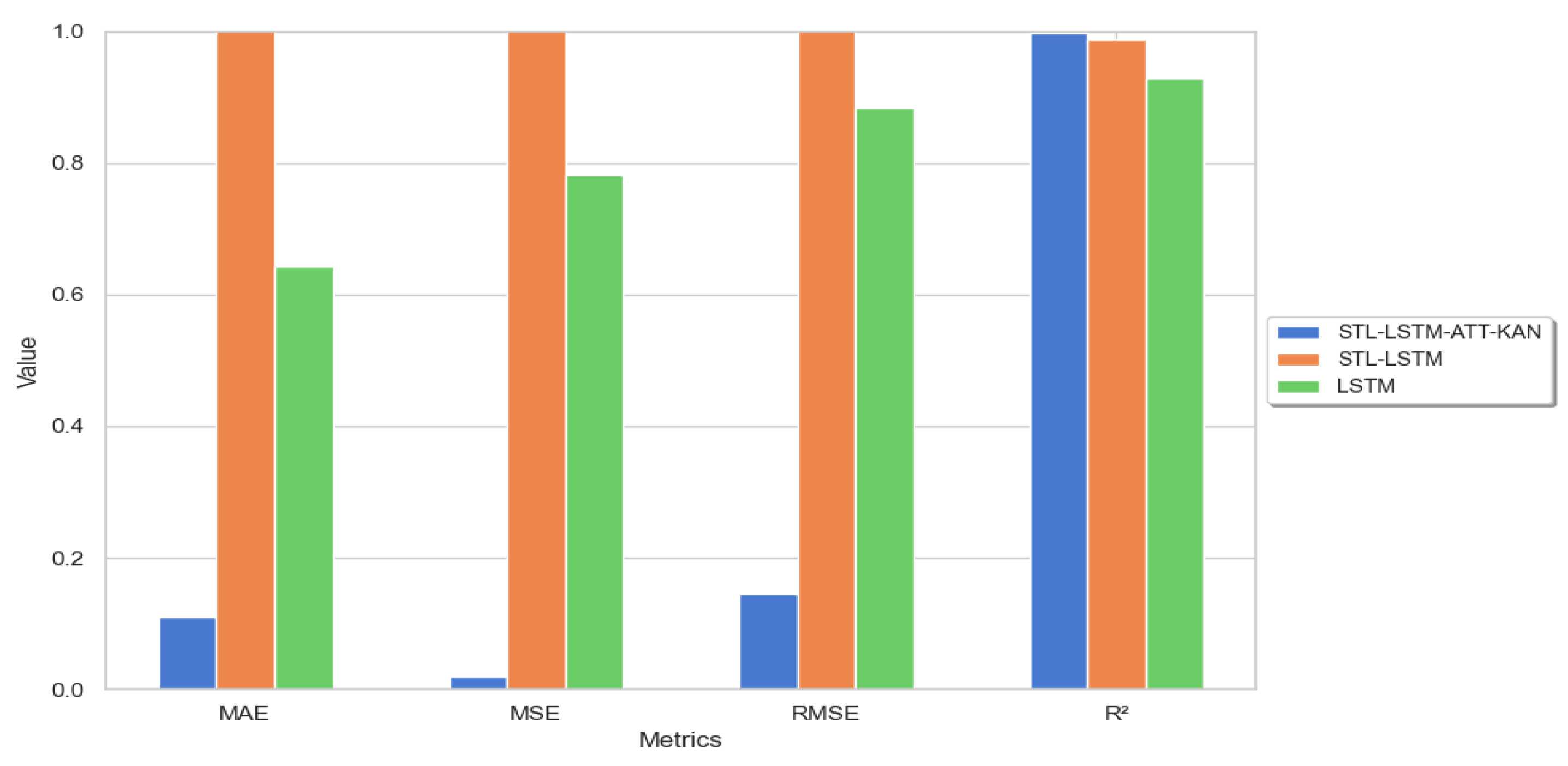

Table 4.
Results of ablation experiments.
| Evaluation Metrics | STL-LSTM-ATT-KAN | STL-LSTM | LSTM |
|---|---|---|---|
| MAE | 0.111 | 1.017 | 0.643 |
| MSE | 0.021 | 5.584 | 0.782 |
| RMSE | 0.146 | 2.363 | 0.884 |
| R² | 0.998 | 0.987 | 0.928 |
The significant decrease in MSE reveals that the combination of ATT and KAN network not only improves the forecasting accuracy, but also strengthens the stability of the model, making it perform better in the face of abnormal volatility. Although the STL-LSTM model lacking ATT and KAN networks still retains the advantages of STL decomposition, it is still inferior to the full STL-LSTM model integrating ATT and KAN networks in terms of error control in complex scenarios. The LSTM model lacking STL decomposition, on the other hand, shows a higher error rate, which further proves the key role of STL in time series feature decomposition.
The significant reduction in RMSE further confirms the overall superiority of the STL-LSTM-ATT-KAN model in time series forecasting. The lower RMSE values indicate that the model is able to provide more accurate forecasts in most cases. Although the RMSE of the STL-LSTM model is lower than that of the standard LSTM model, its prediction results still suffer from a large error due to the lack of enhancement by the ATT and KAN networks. In contrast, the standard LSTM model is unable to decompose the time series efficiently, which leads to the poor stability of its prediction results.
The R² values indicate that both the STL-LSTM-ATT-KAN and STL-LSTM models can excellently elucidate the variance of ginger price fluctuations, which is mainly due to the STL decomposition technique and the LSTM network's accurate capture of the long-term dependence of the time series. However, the R² value of the LSTM model is almost zero, which indicates that it is extremely weak in explaining the ginger price fluctuations without applying the time series decomposition, and the prediction effect is significantly reduced.
The STL-LSTM-ATT-KAN model performs optimally on the evaluation metrics with low MAE, MSE and RMSE values showing its ability to reduce prediction errors. The achievement is attributed to the combination of STL decomposition and the attention mechanism, which improves the prediction accuracy. The increase in error after removing the attention mechanism emphasizes its role in error reduction.The LSTM model, although fitting the data well, does not have as good a prediction accuracy as the STL-LSTM-ATT-KAN, confirming the enhancement of the model performance by the STL decomposition and the attention mechanism.
By applying the STL (Seasonal Trend Decomposition) technique to decompose the time series data, the model is able to handle the trend, seasonality, and residual components independently, which significantly reduces the forecast error. The Long Short-Term Memory Network (LSTM), with its superior ability to capture long-term dependencies in time-series data, enables the model to more accurately handle the long-term trend of ginger prices. Incorporating the attention mechanism in the model allows the model to focus more on key time points during the forecasting process, which improves the accuracy of the forecasts and further reduces the errors.The integration of the KAN network integrates external knowledge sources, improves the generalization ability of the model, and ensures the stability and reliability of the model when dealing with new data.
4. Conclusions
After an in-depth study of the fluctuation patterns of ginger prices and comprehensive consideration of multiple influencing factors, a combined STL-LSTM-ATT-KAN ginger price prediction model was successfully developed. The model is able to accurately capture the linkage effects among markets and reflect the interactions between ginger production and macroeconomics. The model achieves significant improvement in terms of forecast accuracy and stability. This achievement is attributed to the fusion of STL decomposition technique, LSTM network, attention mechanism, and KAN network, as well as the fine optimization in error control and feature processing.
The experimental results clearly reveal the excellent performance of the STL-LSTM-ATT-KAN model in the field of ginger price prediction. The model not only accurately captures the complex nonlinear features of price fluctuations, but also significantly improves the accuracy and comprehensiveness of the prediction. It lays a solid foundation for strengthening the market competitiveness of the ginger industry and stabilizing the price mechanism. At the same time, the model provides reliable data support for the government, helping it to formulate more scientific and rational regulatory policies. In addition, key market participants, such as agricultural traders, farmers, and consumers, also gained valuable information support from the model, which resulted in significant benefits. This study provides a practical tool for accurate forecasting of ginger prices and effectively contributes to the support of market regulation and decision-making. Looking ahead, with the continuous enrichment of data resources and the continuous innovation of technical tools, continuous research will be conducted to improve and refine the model and enhance its application and promotion in the market, in the expectation that it will play a greater role in the prosperous development of the agricultural economy and the stable operation of the market.
Funding
This research was funded by the Shandong Province Higher Education Program for the Introduction and Cultivation of Young Innovative Talents (2021), and the Shandong Province Key Research and Development Program under the Rural Revitalization Science and Technology Innovation Enhancement Action Plan (grant number 2022TZXD0030).
References
- Liu, F.; Wang, R.; Li, C. The application of ARIMA model in the prediction of agricultural commodity prices. Computer Engineering and Application, 2009, 45, 238–239. [Google Scholar]
- Ding, W.; He, Y.; Liu, C. China's corn price fluctuation trend and short-term forecast. Price Theory and Practice, 2014, (04):83-84. [CrossRef]
- Ravishankar, P.; Rakesh, S.; Ranjit, P.K. Price Forecasting of Mango in Varanasi Market of Uttar Pradesh. :218-224.
- Wang, B.; Song, Y.; Zong, Y. Cucumber price trend analysis and market forecast based on ARIMA model. Statistics and Management, 2019, (10):87-90.
- Agriculture - Potato Research; Findings from Ankara University Update Knowledge of Potato Research (Potato Price Forecasting With Holt-winters and Arima Methods: a Case Study). Agriculture Week, 2020, 55-.
- Gestel, V.T.; Suykens KA, J.; Baestaens, D.; et al. Financial time series prediction using least squares support vector machines within the evidence framework. IEEE Trans. Neural Networks, 2001, 12, 809–821. [Google Scholar] [CrossRef] [PubMed]
- Das, M.; Ghosh, S.K. A probabilistic approach for weather forecast using spatio-temporal inter-relationships among climate variables [C]//2014 9th International Conference on Industrial and Information Systems (ICIIS). IEEE, 2014: 1-6.
- Duan, Q.; Zhang, L.; Wei, F.; et al. Forecasting model and validation of aquatic product price based on time series GA-SVR. Journal of Agricultural Engineering, 2017, 33, 308–314. [Google Scholar]
- Wang, P.; Zhang, H.; Qin, Z.; et al. A novel hybrid-Garch model based on ARIMA and SVM for PM2. 5 concentrations forecasting. Atmospheric Pollution Research, 2017, 8, 850–860. [Google Scholar] [CrossRef]
- Polyiam, K.; Boonrawd, P. A hybrid forecasting model of cassava price based on artificial neural network with support vector machine technique[C]. IEEE, 2017:123-127. [CrossRef]
- Zhao, B.; Huo, Q.; Lu, Y. Research on the characteristics of ginger price fluctuation and its law -an analysis based on ARCH class model. Price Theory and Practice, 2022, (05): 130-133.
- Teng, J.; Liu, P.; Zhang, Y.; Xu, S.; Xu, G.; Han, W. A study on ginger price prediction based on Prophet. Chinese Journal of Agricultural Chemistry, 2020, 41, 211–216. [Google Scholar]
- Wang, Y. Research on the combination prediction model of ginger price based on multiple influencing factors [D]. Shandong Agricultural University, 2023.
- Lv, X. Research on Price Forecasting of Small Agricultural Products Based on the Influence of Network Public Opinion[D]. Northeast Agricultural University, 2023.
- Raj, C.; Nath, H.G.; Raj, N.B.; et al. An analysis of the ginger value chain in palpa, Nepal. Cogent Food Agriculture 2023, 9. [Google Scholar]
- Manjubala, M. Weekly price prediction of garlic and ginger using complex exponential smoothing. 2023.
- Li, H.; Jia, Y.; Zhang, Y. Research On Pricing Strategies Based on Time Series Analysis Model and Greedy Algorithm Model. Highlights in Business, Economics and Management 2024, 25, 127–133. [Google Scholar] [CrossRef]
- Fu, L.; Zhang, H. Analysis of Price Influencing Factors of Small-Scale Agricultural Products Based on Network Perspective. 2023.
- Anamisa Devie Rosa; et al. Long Short-Term Memory Method Based on Normalization Data For Forecasting Analysis of Madura Ginger Selling Price[C], 2023.
- Lin, S.; Runger, C.G. GCRNN: Group-Constrained Convolutional Recurrent Neural Network. IEEE Trans. Neural Netw. Learning Syst. 2018, 29, 4709–4718. [Google Scholar] [CrossRef] [PubMed]
- Hu, L.; Li, J.; Nie, L.; et al. What Happens Next? Future Subevent Prediction Using Contextual Hierarchical LSTM[C]. 2017. [CrossRef]
- Zhang, Y.; Yang, X.; Ivy, J.; et al. ATTAIN: Attention-based Time-Aware LSTM Networks for Disease Progression Modeling[C]//Twenty-Eighth International Joint Conference on Artificial Intelligence {IJCAI-19. 2019. [CrossRef]
- Liu, Z.; Wang, Y.; Vaidya, S.; et al. Kan: Kolmogorov-arnold networks. arXiv 2024, arXiv:2404.19756, preprint. [Google Scholar]
- Zhi, L.; Zuo, Y. Collaborative Path Planning of Multiple AUVs Based on Adaptive MultiPopulation PSO. (2).
Figure 1.
STL-ATT-LSTM-KAN model structure.
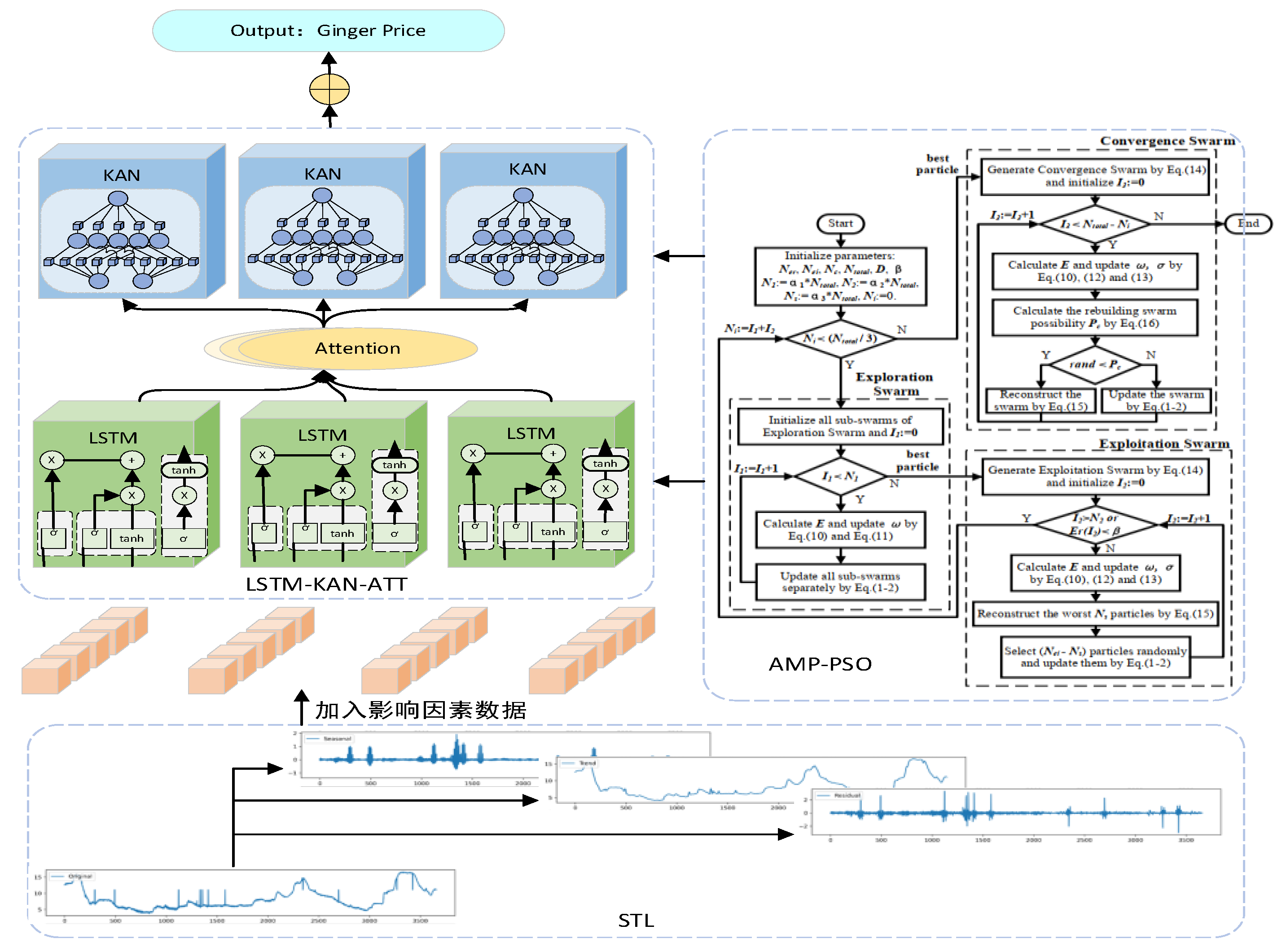
Figure 2.
Structure of LSTM network.
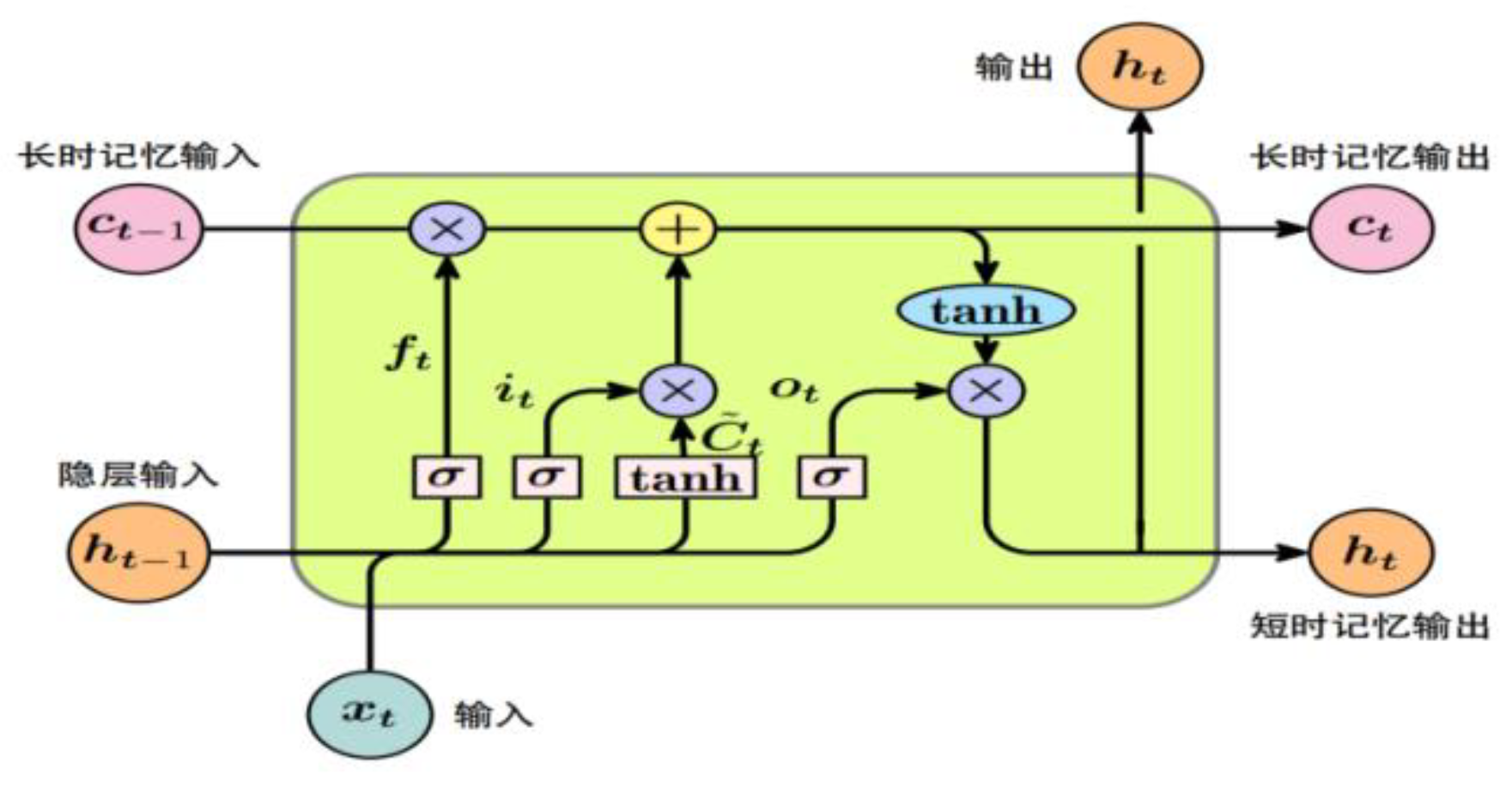
Figure 3.
Structure of the attention mechanism.

Figure 4.
KAN network structure.
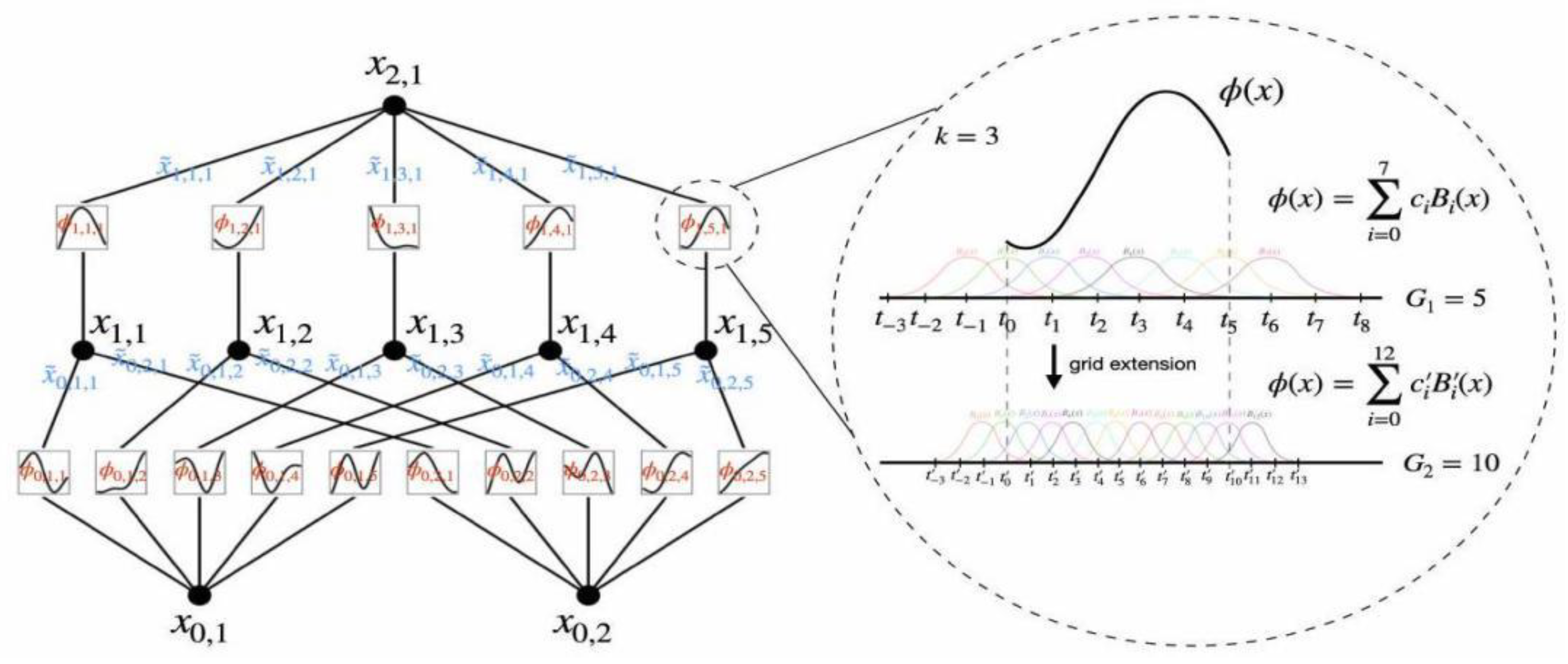
Figure 5.
Exploded view of STL time series.
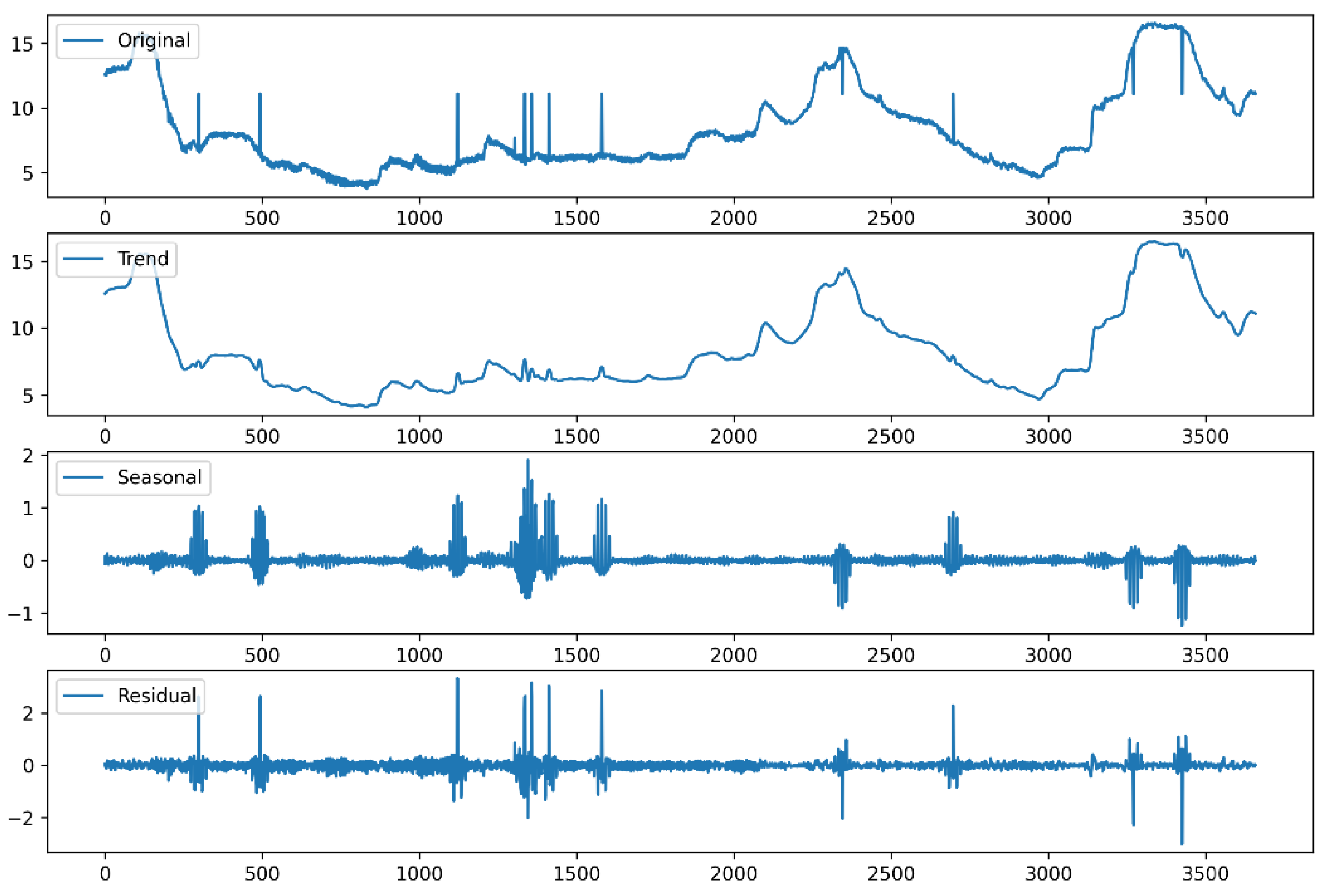
Figure 6.
Training loss curve.
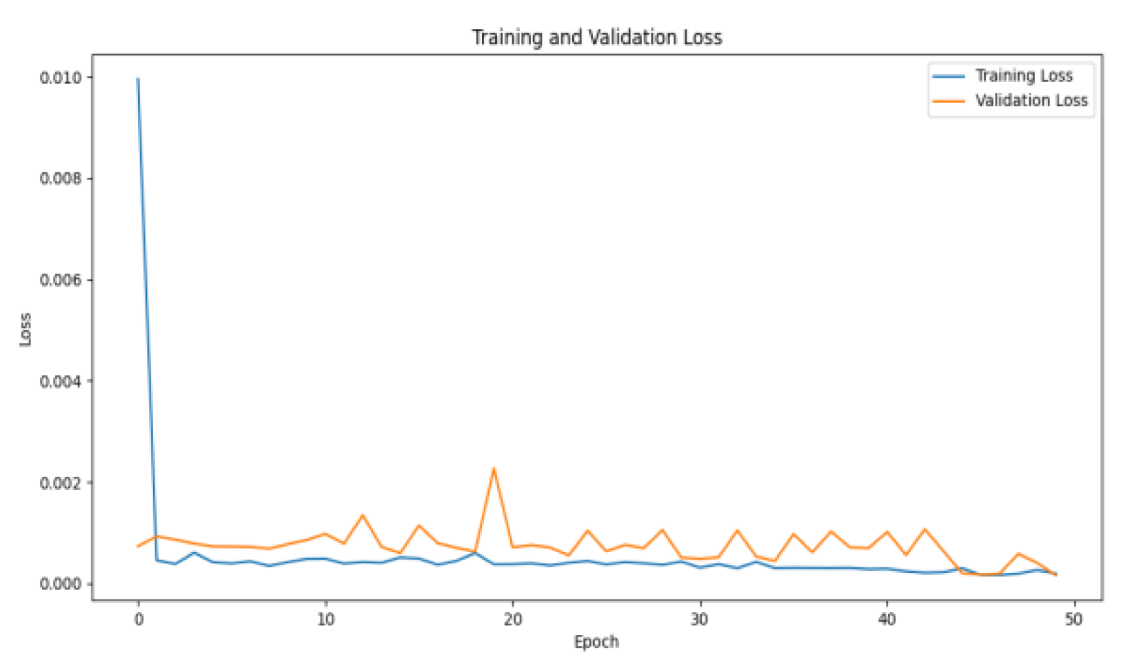
Figure 7.
Model residual plot.
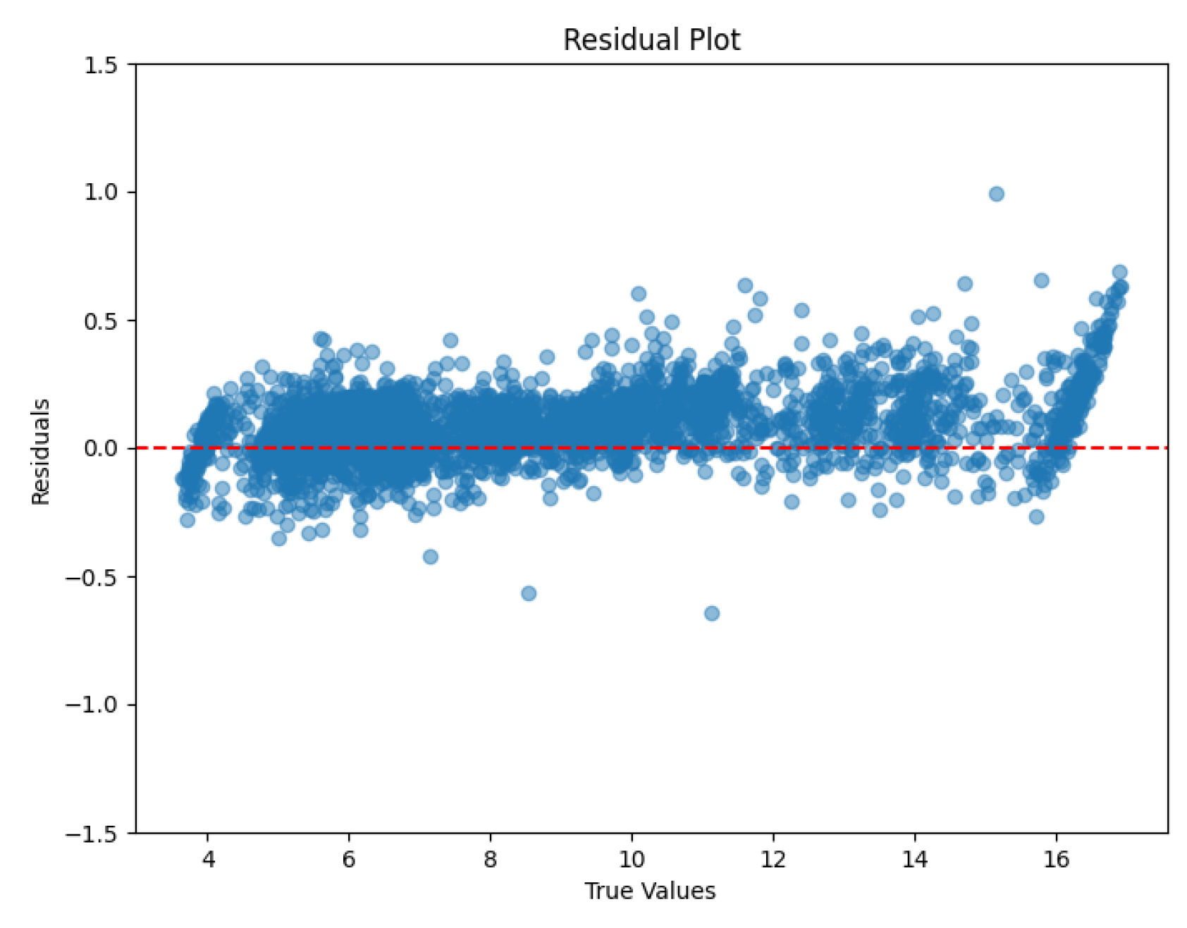
Figure 8.
Comparison of true value prediction trends.
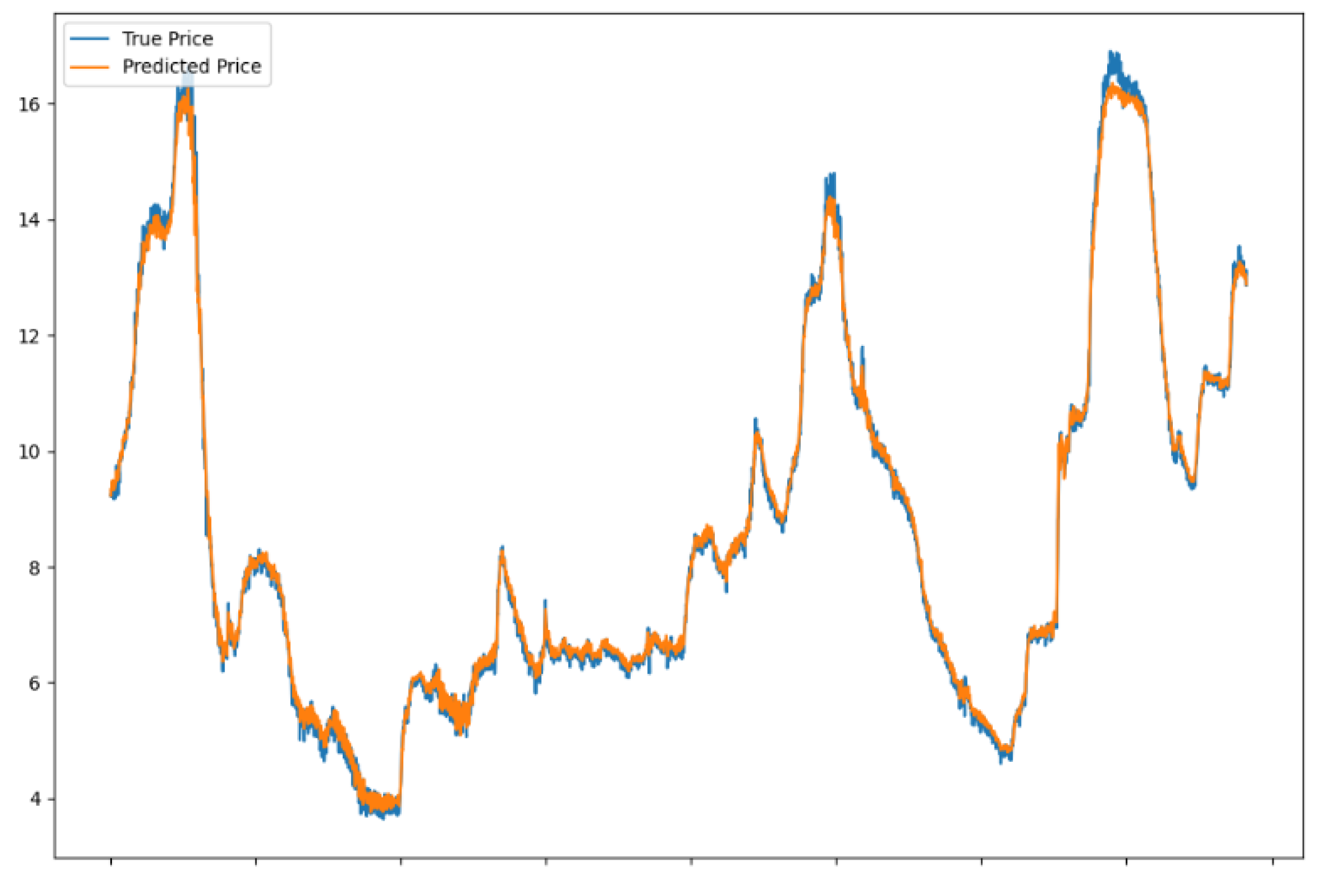
Figure 9.
Forecast trend for the future seven days.
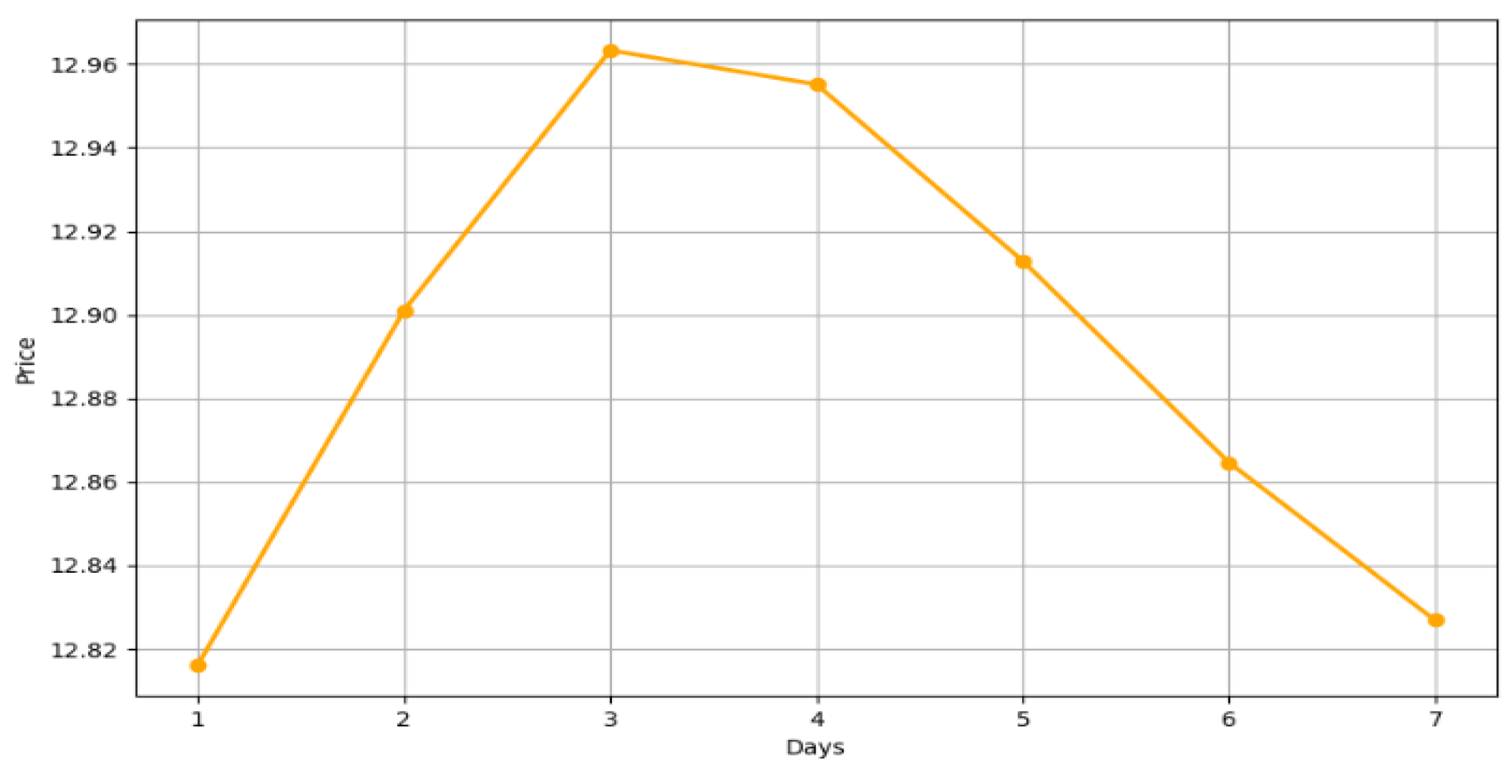
Figure 10.
Comparison of prediction results.
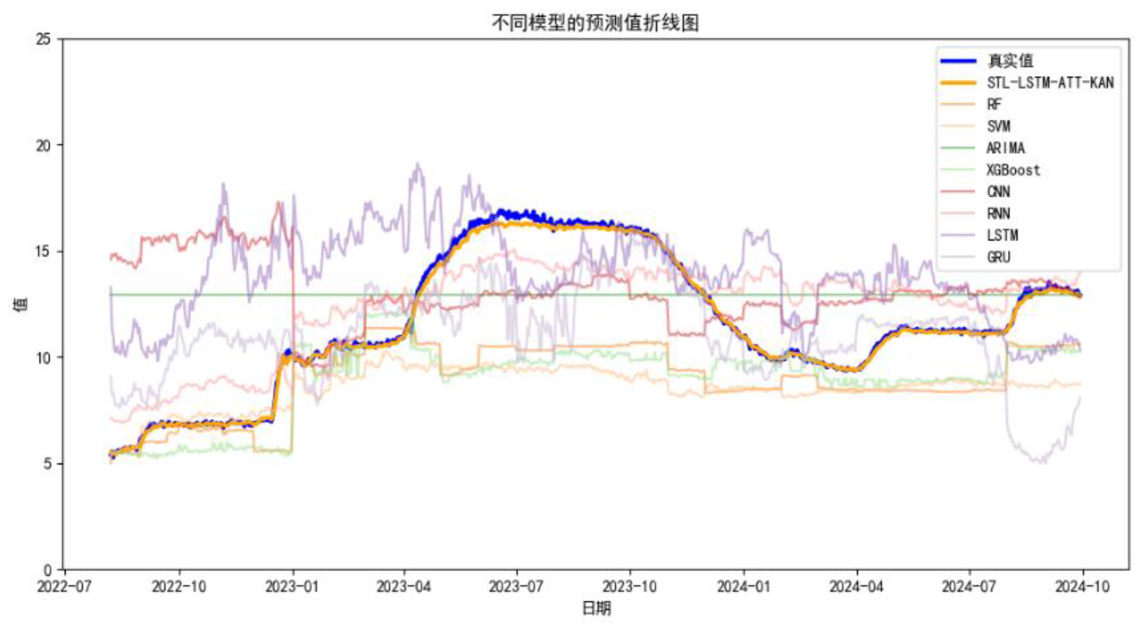
Figure 11.
Comparison error bar chart.
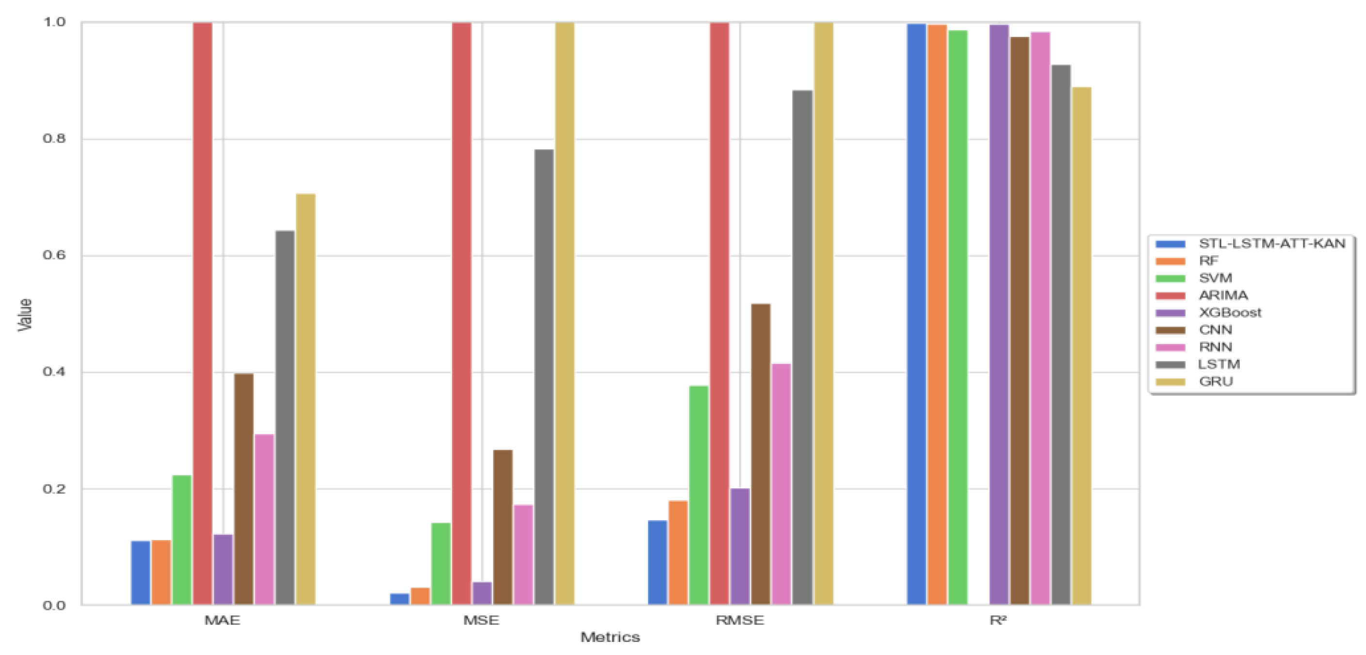
Table 1.
Key influences on ginger prices.
| Level 1 impact factors | Specific influencing factors |
|---|---|
| Agricultural price factors | Average daily price of garlic |
| Average daily price of onions | |
| Agricultural production factors | Average daily temperature in the main ginger producing areas |
| Area under cultivation (10,000 acres) | |
| Harvested area (annual) | |
| Production (tons) | |
| production volume index | |
| Economic indicator factors | Consumer Price Index (CPI) for Fresh Vegetables |
| Broad money supply M2 | |
| Exchange rate (USD/CNY) | |
| Disposable income of the population | |
| International market factors | export amount |
| export volume | |
| International crude oil prices | |
| Market Opinion Factors | Ginger Opinion |
Table 2.
AMP-PSO parameter selection.
| model parameter | parameter value |
|---|---|
| kan_units | 22 |
| lstm_units | 50 |
| learning_rate | 0.004 |
| batch_size | 36.451 |
Table 3.
Comparative experimental results.
| Evaluation Metrics | STL-LSTM-ATT-KAN | RF | SVM | ARIMA | XGBoost | CNN | RNN | LSTM | GRU |
|---|---|---|---|---|---|---|---|---|---|
| MAE | 0.111 | 0.113 | 0.224 | 4.692 | 0.123 | 0.398 | 0.295 | 0.643 | 0.707 |
| MSE | 0.021 | 0.032 | 0.143 | 27.864 | 0.0409 | 0.268 | 0.1737 | 0.782 | 1.195 |
| RMSE | 0.146 | 0.181 | 0.378 | 5.278 | 0.202 | 0.518 | 0.416 | 0.884 | 1.093 |
| R² | 0.998 | 0.996 | 0.986 | -1.549 | 0.996 | 0.975 | 0.984 | 0.928 | 0.890 |
Disclaimer/Publisher’s Note: The statements, opinions and data contained in all publications are solely those of the individual author(s) and contributor(s) and not of MDPI and/or the editor(s). MDPI and/or the editor(s) disclaim responsibility for any injury to people or property resulting from any ideas, methods, instructions or products referred to in the content. |
© 2025 by the authors. Licensee MDPI, Basel, Switzerland. This article is an open access article distributed under the terms and conditions of the Creative Commons Attribution (CC BY) license (http://creativecommons.org/licenses/by/4.0/).
Copyright: This open access article is published under a Creative Commons CC BY 4.0 license, which permit the free download, distribution, and reuse, provided that the author and preprint are cited in any reuse.


