
Submitted:
09 February 2025
Posted:
10 February 2025
You are already at the latest version
Abstract
The proliferation of IoT devices in smart environments has brought significant challenges related to device management, security, and communication integrity. Effective classification and recognition of these devices are crucial for enhancing management processes, strengthening security protocols, and ensuring seamless communication. This study compares Gradient Boosting (GB) and Random Forest (RF) classifiers using a dataset containing network traffic data from 1,900 smart home devices. The classifiers were evaluated based on their ability to categorize devices into ten distinct categories, each representing a specific type or function of IoT devices. Utilizing performance metrics such as accuracy, precision, recall, MCC (Matthews Correlation Coefficient), F1-score, and AUC (Area Under the Receiver Operating Characteristic Curve), both models demonstrated strong classification capabilities through 20-fold cross-validation.
Results indicated that Gradient Boosting achieved a precision of 92%, recall of 90%, and an F1-score of 91%, slightly outperforming Random Forest, which recorded a precision of 89%, recall of 87%, and an F1-score of 88%. However, Random Forest demonstrated superior performance in AUC with a score of 0.94, excelling in distinguishing specific device types. Both models encountered challenges in classifying devices with overlapping features, underscoring the necessity for further feature refinement and tuning. The ROC curve analysis provided insights into the actual positive rate versus false positive rate trade-offs, while confusion matrices highlighted specific categories where misclassifications occurred. This study underscores the potential of integrating advanced machine learning techniques to improve IoT device classification and facilitate smarter, more secure environments.
Keywords:
Smart environments
; IoT
; Random Forest
; Gradient Boosting
; Classification
1. Introduction
The Internet of Things (IoT) connects billions of items, including home appliances and traffic management systems, via sensors and communication protocols such as Wi-Fi, Bluetooth, ZigBee, and Ethernet. Data-based insights, automation, and increased productivity are all fueled by this interconnected network in various industries. Through communication, data sharing, and decision-making coordination, IoT enables physical things to perceive, process, and perform activities. The large variety of communication protocols demonstrates how IoT devices can be tailored to various settings and use cases. This helps explain why they are so widely used in both sectors and daily life. IoT devices connected in "smart environments" have significantly changed several industries, affecting security, welfare, comfort, and human safety [1,2,3,4,5].
This paper determines how IoT transforms smart environments, emphasizing the interconnectedness of devices that enable efficiency and innovation across diverse sectors.
Smart Environment
The environment is vital for all life forms but faces threats from pollution, resource wastage, industrial activities, and transportation emissions. Innovative solutions are needed to monitor and manage waste and provide data to drive effective environmental protection policies. Integrating IoT technology into smart environment strategies offers tools for sensing, tracking, and analysing environmental factors, promoting sustainable living [6]. IoT enables applications such as air quality monitoring through distributed sensors, improving urban traffic management and providing continuous geographic coverage. The goal of smart environments is to enhance human comfort and efficiency. IoT has become a cornerstone in developing smart environments, including smart cities, homes, agriculture, and healthcare, by facilitating automated network communication to deliver diverse services. [7]. Here are brief definitions for various smart environments:
- Smart Cities: These use IoT technology and data analytics to improve urban living. With a growing global population, cities consume 75% of natural resources and contribute 60-80% of global greenhouse gas emissions, leading to resource depletion and global warming. The smart city concept addresses human needs and environmental concerns, enhancing the quality of life and social well-being [8].
- Smart Homes: is a system where appliances and devices can be controlled remotely using an internet connection, allowing homeowners to manage security, climate control, lighting, and entertainment systems from a distance. Smart doorbells, security systems, and appliances form part of the IoT ecosystem, collecting and sharing information. A smart home offers greater comfort, security, and environmental sustainability. Intelligent air conditioning systems use home sensors and online data sources to optimise operational decisions, forecasting home occupancy and conserving energy [3,9].
- Smart Agriculture: uses IoT sensors, GPS technology, and data analytics to monitor crop health, soil conditions, and livestock, resulting in optimised resource use, increased productivity, and sustainable practices. It goes beyond incorporating technology; agricultural machinery and equipment should have IT capabilities for semi-automated decision-making. This approach relies on big data technologies, IoT, satellite monitoring, interconnected data, and artificial intelligence [7,10].
- Smart Healthcare Systems: These systems utilize IoT devices and data analytics to monitor patient health, manage medical records, and enhance healthcare delivery efficiency. They include remote patient monitoring, telemedicine, and intelligent diagnostic systems. IoT can record patient data, generate diagnostic reports, and detect vital signs. Wearable devices like Fitbit and smart watches monitor physical activity, allowing users to set activity targets and track their health goals. This proactive approach saves time for patients and reduces healthcare costs [7,11].
Building on the above introduction to smart environments, this article investigates the implementation of Random Forest (RF) and Gradient Boosting (GB) for efficiently classifying smart home objects. Classification is crucial in categorizing various objects, behaviors, and activities, enhancing automation and decision-making within smart environments.
In diverse IoT environments, various classifiers categorize smart devices based on different attributes. This study presents recent publications that utilized two or more classification methods, including Random Forest or Gradient Boosting, within smart environments.
The study [12] focuses on early cardiac arrest detection and patient monitoring using an advanced wearable device. This system leverages hybrid computing, combining cloud and edge computing, to achieve fast response times and low latency, which are crucial for timely cardiac monitoring.
In this article, the authors propose a wearable device paired with an Android application that collects real-time data from sensors attached to the patient. The system then analyses heart health data using three machine learning models: Support Vector Machine (SVM), Adaptive Boosting (AdaBoost), and Random Forest (RF), which are chosen for their accuracy in classification tasks. By optimizing performance metrics like accuracy, error rate, and response time, the system aims to ensure rapid detection of cardiac anomalies, allowing healthcare providers to respond quickly to potential emergencies. The study shows promising results, suggesting that such a wearable system could significantly aid in remote cardiac health monitoring, potentially preventing sudden cardiac events and supporting daily patient care without intruding [12].
The paper [13] explores the integration of homomorphic encryption with machine learning (ML) to enhance privacy in smart home environments. Specifically, the study examines the performance of ML models XGBoost, Random Forest, and Decision Classifier for activity recognition when applied to homomorphically encrypted data from real-world smart home datasets. The authors focus on preserving users' privacy by employing homomorphic encryption, which enables computations on encrypted data without decryption, thus maintaining data security. This approach detects and classifies user activities within a smart home setting, where data from sensors and IoT devices are typically sensitive. The study provides insights into the feasibility of privacy-preserving activity recognition by comparing various ML models' accuracy and computational efficiency on encrypted vs. unencrypted data. It offers valuable findings on the trade-offs between data privacy and model performance. The case study demonstrates the potential for homomorphic encryption to safeguard privacy in smart environments while supporting effective ML-based activity recognition [13].
The authors in [14] investigate using advanced machine learning algorithms to forecast solar irradiance, a crucial factor for smart grid management. They found that MLP-ANNs perform better when combined with PCC-based feature selection, with the random forest algorithm being the most accurate.
To assess their forecasting performance, the paper evaluates several advanced machine learning models, including Random Forest, XGBoost, LightGBM, CatBoost, and Multilayer Perceptron Artificial Neural Networks (MLP-ANN). They employ Bayesian optimization for fine-tuning hyperparameters, which significantly improves model accuracy. A notable finding is that the Random Forest algorithm outperforms others, achieving the best prediction accuracy for solar irradiance, mainly when feature selection is applied to MLP-ANN models. This research highlights the importance of machine learning in enhancing solar power utilization for cleaner energy management in smart grids [14].
The article [15] evaluates six advanced boosting-based algorithms for detecting intrusions in IoT, analyzing their performance in multi-class classification, accuracy, precision, detection rate, F1 score, and training and testing times. It explores how different boosting-based machine learning algorithms can effectively detect intrusions in IoT networks. Boosting algorithms, such as AdaBoost, Gradient Boosting, and XGBoost, are known for enhancing prediction accuracy by combining multiple weak models to form a robust model. The study compares these algorithms to determine their efficiency, accuracy, and computational requirements in identifying security threats within IoT environments. The findings highlight which algorithms are most suitable for intrusion detection tasks, focusing on the specific challenges of IoT networks, such as limited computational resources and high data variability.
This comparative analysis helps address the unique challenges of IoT environments and aims to advance the effectiveness of intrusion detection systems tailored for IoT networks. [15]
The study [16] presents a novel approach using hyperparameter-tuned Machine Learning classifiers with Optuna for fault detection and classification over a power transmission line. Popular models like Random Forest, Decision Tree, XGBoost, and Light Gradient Boosting Machine are used. The study uses a two-layer approach, extracting optimal features from 3-phase current and voltage signals. The research enhances fault detection accuracy by tuning hyperparameters for classifiers like decision trees and SVMs while minimizing computational demands, making it ideal for energy-constrained environments like IoT networks.
In the methodology, machine learning classifiers are tuned for energy-efficient fault detection and classification in sensor-based systems. The models are evaluated for their accuracy, energy consumption, and robustness in classifying faults within the system. This methodology reduces energy demands and enhances fault detection in smart and industrial environments. The findings support the development of more sustainable and efficient sensor networks for real-time fault management. [16]
The paper [17] focuses on improving the reliability and accuracy of smart meters in smart grid systems by forecasting their status and classifying faults. The authors address challenges with smart meter malfunctions, which can disrupt data collection and lead to inefficiencies in energy management. The study investigates the impact of a random forest algorithm on smart meters' state prediction and fault classification, aiming to improve their stability. The researchers analyze the theoretical basis and application of the Random Forest and Light Gradient Boosting Machine algorithms. They design an improved fault classification and state prediction model using public data sets, achieving high accuracy and recall rates.
The work presents an approach for status prediction using the LightGBM (Light Gradient Boosting Machine) algorithm, a fast and efficient machine learning model. This model is improved with the Random Forest algorithm to enhance its accuracy and robustness in classifying various types of faults in smart meters. The combination leverages LightGBM's high-speed performance and Random Forest's robustness to handle different fault types effectively. The results demonstrate that the hybrid approach offers improved prediction accuracy and fault classification, making it helpful in managing and maintaining smart meter operations in real-world smart grid applications. [17]
The authors of [18] present a two-stage classification framework for identifying IoT devices in a smart city context. The framework uses network and statistical features to characterize devices and achieves 99% accuracy. The first stage uses Logistic Regression, which investigates the association between independent and dependent variables. The goal is to estimate the probability X for a combination of the independent variables.
The second stage uses a gradient boosting algorithm, which takes all quantitative features such as packet interarrival time, traffic flow rates, burstiness rate, packet length, IP source address, IP destination address, and TTL, along with the output from the stage 0 classifier. The gradient boosting algorithm finds the optimal initial prediction using a differentiable loss function and the number of iterations n. The model is updated according to its output, and the testing data is classified into the abovementioned classes.
The evaluation results show that the proposed classification can achieve 99% accuracy compared to other techniques, with a Mathews Correlation Coefficient of 0.96.1[18].
To this end, considering previously discussed smart environments and the literature of some recent studies that employed Random Forest (RF) and Gradient Boosting (GB), this study aims to explore integrating two distinct classification technologies to improve the accuracy of object classification in smart environments.
This article aims to achieve these objectives by investigating the use of Random Forest (RF) to categorize smart home objects and improve RF accuracy by applying Gradient Boosting (GB). The structure of this article is presented next.
2. Paper Structure
The structure of the paper is as follows: Section 2 outlines the methodology for employing Random Forest and gradient-boosting classifiers to categorize smart home devices. Section 3 and Section 4 include an analysis and discussion of evaluating the performance of these classifiers. Finally, Section 5 concludes the paper and presents recommendations for future research.
2.1. The Methodology
This section outlines the stages of investigating the use of Random Forest and gradient-boosting classifiers for categorizing smart home devices. It includes details about the data source, a brief dataset description, and information regarding the target variable. Additionally, it highlights the classification techniques, provides foundational concepts, and offers an overview of Random Forest and gradient boosting, which were employed in this study.
2.2. Fundamentals of Classification
Classification is grounded in supervised learning (SL), a significant branch of machine learning (ML), alongside unsupervised, semi-supervised, and reinforcement learning. ML, a subset of artificial intelligence (AI), uses statistical methods to enable computers to learn from data and make decisions. Supervised learning trains models on labelled datasets and includes two primary types:
- -
- Regression: This technique analyzes the relationship between target (dependent) and predictor (independent) variables. It predicts continuous numerical values by modelling this relationship, making it useful for forecasting and trend analysis tasks.
- -
- Classification: Assigns data to predefined categories or labels by identifying patterns in input features. It predicts discrete outcomes and applies to structured and unstructured data.
While both classification and regression are vital for prediction tasks, their distinction lies in their output; classification deals with discrete categories, while regression predicts continuous values. Together, they are integral to solving real-world problems in supervised learning. [19,20]
Classification encompasses four primary task types: binary classification, multi-class classification, multi-label classification, and imbalanced classification. Each task type can be addressed using different algorithms, with an algorithm tailored to the specific dataset and application. Here are some commonly used classification algorithms and techniques [20].
Several classifiers are used in machine learning, each suited to specific data types and classification tasks. Here is an overview of Random Forests (RF) and Gradient Boosting (GB), which are essential to understand before diving into the details of the methodology:
- A.
- Random Forest (RF):
A Random Forest (RF) classifier is a collection of decision trees, each built with an element of randomness. At the leaf nodes of each tree, labels reflect estimates of the posterior distribution for classes, while internal nodes perform tests that optimally divide the data to be classified. RF is suitable for binary, multi-class, and imbalanced classification.
The number of trees required for effective performance typically increases with the number of predictors. The best way to determine the ideal number of trees is by comparing the predictions from the entire forest with those from a subset; when the subset performs as well as the whole forest, it suggests an adequate number of trees. Many trees are essential for stable estimates of variable importance and proximity. Since the algorithm is highly parallelizable, it’s feasible to run separate RF models on different machines and then combine their votes for the final result. In addition, RF classifiers add further randomness by altering how classification or regression trees are constructed. While standard trees use the best split across all variables for each node, RF trees split each node using the best option within a random subset of predictors. [21]
The algorithm's output is determined by the average or majority vote from the individual trees. Mathematically, the Random Forest model’s output for a new sample, for classification and regression [22] is presented by Equation (1):
where Is the number of decision trees and Is the prediction of the decision tree for input.
As illustrated in Figure 1, the random forest algorithm is built through three primary steps: creating training sets, constructing decision trees, and then forming and executing the final algorithm. Given that a random forest is composed of Trees: the algorithm requires Individual decision trees for training. To accomplish this, an equivalent number of training sets must be generated. To reduce the likelihood of decision trees reaching only locally optimal solutions, random forest employs the bagging method, a random sampling approach with replacement to produce Sets of training samples. This method inevitably results in repeated samples within the generated training sets [17].
The Random Forest (RF) algorithm has numerous benefits, such as effectively handling large datasets, maintaining stability, and resisting noise and outliers. However, RF has some limitations, including longer training times than other machine learning algorithms, higher complexity that demands more computational resources, and slower real-time predictions [20].
RF finds extensive application across various fields, including practical, real-world cases. For instance, it can be used in finance to evaluate loan applicants' risk levels, categorizing them as high or low. Additionally, RF can predict potential failures in mechanical components of automobile engines, estimate social media engagement scores, and analyze performance indicators [20].
- B.
- Gradient Boosting Machines (GBM):
In a Gradient Boosting Machine (GBM), multiple weak classifiers are combined to form a robust predictive model. The technique is typically based on decision trees, generating independent trees that can take longer to execute. The model iteratively refines its performance through probability approximately correct (PAC) learning, adapting and optimizing with each step to improve accuracy. GBM is effective on raw data and can efficiently manage missing values by leveraging differentiable loss functions, which allow it to adapt to various tasks without requiring a custom loss function every time [23].
GBM tuning involves several hyperparameters to enhance model accuracy, such as setting the number of trees (e.g., `n = 100`), meaning that predictions are averaged over 100 trees for robust results. Additionally, a `max depth` value limits tree depth to 60 in this case to control model complexity. In classification tasks, GBM often utilizes logarithmic loss to quantify prediction error, enabling it to perform competitively against regression-based methods [23].
XGBoost (eXtreme Gradient Boosting) and LightGBM (Light Gradient Boosting Machine) use boosting techniques to improve predictive performance instead of Random Forest's bagging approach. Derived from Gradient Boosting, these models train numerous weak learners sequentially, with each model focusing on errors made by its predecessor. This iterative process minimizes the loss function representing the difference between predicted and actual values, achieved through gradient descent optimization.
XGBoost combines tree-based boosting with parallel processing, enhancing accuracy and computational speed, especially on large datasets with extensive attributes. LightGBM, a later development, applies a leaf-wise growth strategy, boosting parallel training efficiency, lowering memory requirements, and supporting distributed computing. These characteristics make LightGBM especially suitable for handling large, complex datasets. [24]
2.3. Data Source and Description
This study uses a dataset from Chapter 5 of the “Machine Learning Cookbook for Cyber Security,” found at [25]. It contains network traffic analysis data from a smart home appliance featuring a range of IoT devices and was initially created by other researchers.
The dataset contains 1900 rows × 298 columns. Each row corresponds to a single data point or observation, which, in this case, likely represents a single IoT device. Therefore, the dataset contains information about 1900 different IoT devices. Each column represents the IoT devices' specific feature or attribute, including the target variable 'device_category.' Your dataset includes 298 features or attributes for each IoT device and its category label. The target variable `'device_category'` consists of ten different categories: `'baby_monitor'`, `'lights'`, `'motion_sensor'`, `'security_camera'`, `'smoke_detector'`, `'socket'`, `'thermostat'`, `'TV'`, `'watch'`, and `'water_sensor'`. These categories will be used in the classification process to assign each data point to its appropriate category.
2.4. Optimized Classifier Selection for Smart IoT Environments
Choosing an appropriate classifier is essential in fast-growing IoT environments where interconnected devices generate vast amounts of data, requiring efficient processing, storage, and classification to ensure system responsiveness and scalability. This study selected Random Forest (RF) and Gradient Boosting for categorizing smart objects due to their robustness, ability to manage high-dimensional data, and effectiveness with complex, non-linear relationships. RF offers strong performance and reduces overfitting by averaging decision trees. At the same time, Gradient Boosting enhances accuracy through iterative error correction, making these methods ideal for dynamic data within smart environments.
RF was used to categorize data into classes of the target variable “device_category” and was further enhanced with Gradient Boosting. Both classifiers were initialized and tested with 20-fold cross-validation, a robust evaluation method alongside Train-Test Split and Leave-Out-Out Validation. In 20-fold cross-validation, the dataset is divided into 20 equal parts; for each part, the classifier is trained on the remaining parts, and the average error rate across folds estimates the classifier's overall accuracy [26]. After testing, the following section evaluates classifier performance using various performance metrics.
2.5. Performance Measurement Matrices
In machine learning, classification tasks with more than two categories are called "multi-class classification." Performance indicators are crucial in assessing and comparing various classification models or techniques. A range of metrics is available to evaluate the effectiveness of a multi-class classifier. In multi-class classification, the response variable and the prediction can be treated as discrete random variables, each taking values in the set , where each number corresponds to a distinct class. The algorithm calculates the probability that a given instance belongs to each possible class, after which a classification rule assigns a specific class. Typically, this rule is straightforward, with the most common approach being to assign the instance to the class with the highest probability [27].
Various metrics are available to assess the effectiveness of any multi-class classifier, making it easier to compare the performance of different models or analyze how a single model behaves when parameters are adjusted. Many of these metrics are derived from the Confusion Matrix, which contains essential details on the algorithm's performance and classification accuracy [27].
A. Confusion matrix
The confusion matrix is an essential tool for assessing the performance of classification models, particularly in multi-class classification tasks. It offers a comprehensive view of how effectively a model differentiates between various classes by displaying a matrix that summarizes:
- -
- True Positive (TP): A data point is classified as a True Positive (TP) in the confusion matrix when a positive outcome is predicted and the actual result matches the prediction.
- -
- False Positive (FP): A data point is classified as a False Positive (FP) when a positive outcome is predicted, but the actual outcome is negative. This is known as a Type 1 Error, where the prediction is overly optimistic.
- -
- False Negative (FN): A data point is classified as a False Negative (FN) when a negative outcome is predicted, but the actual outcome is positive. This is referred to as a Type 2 Error and is considered problematic as a Type 1 Error.
- -
- True Negative (TN): A data point is classified as a True Negative (TN) in the confusion matrix when a negative outcome is predicted and the actual result is negative.
In the case of multi-class classification, each row of the matrix corresponds to instances from an actual class. At the same time, each column represents instances predicted as belonging to a particular class [27,28,29].
B. Evaluation matrices
As we work with IoT data to ensure more comprehensive and insightful results, the performance of the two classification techniques chosen for this study was evaluated using essential standard metrics. These metrics help assess algorithm efficiency and enable a comparative analysis. They include [30]:
- Accuracy: This metric represents the ratio of correctly classified data points to the total number of observations.
- Precision: Precision answers the question: What proportion of predicted positives were correct? In other words, it measures how often the model is correct when it predicts an item to belong to a particular class.
- Recall: Also known as Sensitivity, this metric indicates how many positive class predictions were made from all the actual positive instances in the dataset.
- F-Measure: The F-Measure combines precision and recall into a single score, offering a balanced evaluation of the model’s performance. The The score considers precision and recall at equal weights, returning values between 0.0 and 1.0. [30]
- Area Under the Curve (AUC): is a performance metric used in classification tasks.
- Matthews Correlation Coefficient (MCC): is a measure of the correlation between the predicted classes and the actual ground truth. MCC is widely regarded as a balanced metric, making it suitable even when the classes have significantly different sizes [29].
Equations (2), (3), (4), (5), and (6) can calculate the metrics for accuracy, precision, recall, MCC, and F1-score, respectively. These are all derived from the confusion matrix values [29,31].
The next part will represent the performance analysis for each classifier, including evaluations of the proposed models using various performance metrics.
3. Results Analysis and Discussions
The aim is to evaluate both models' performance, features, and outcomes. By assessing their methodologies, architectures, and results, this analysis provides insights into each model's relative strengths and weaknesses and their efficacy and reliability in real-world applications. Ultimately, this comparison informs decision-making processes regarding selecting appropriate models for IoT device classification tasks.
3.1. Comparison of Overall Performance for Both Methods
As noted in the previous section, the performance of the two classification techniques selected for this study was evaluated using standard metrics: accuracy, precision, recall, MCC, F1-score, and AUC. The classification results of both models, based on 20-fold cross-validation for all the performance metrics, are presented in the tables below.
The performance results of both models for classifying the ten target classes, as shown in Table 1 and Table 2, demonstrate that the Gradient Boosting model generally outperformed the Random Forest model, achieving higher AUC and F1 scores across most classes. However, both models exhibited limitations in classifying certain classes, such as Lights, Water Sensor, and Socket, where they recorded low F1 scores, recall, MCC, and precision. A detailed comparison of results for each class is outlined below:
- ➢
- TV: Both models demonstrated high accuracy, with Random Forest slightly outperforming Gradient Boosting regarding precision and recall.
- ➢
- Baby Monitor: Both models performed exceptionally well, with Gradient Boosting achieving a slightly higher F1 score.
- ➢
- Lights: Both models faced challenges with this class, exhibiting low F1 scores, recall, MCC, and precision.
- ➢
- Motion Sensor: Both models performed well, with Gradient Boosting showing a slight advantage.
- ➢
- Security Camera: Both models achieved optimal performance with high scores across all metrics.
- ➢
- Smoke Detector: Both models performed well, with Gradient Boosting achieving a slightly higher F1 score.
- ➢
- Socket: Both models struggled with this class, exhibiting low F1 scores, recall, MCC, and precision.
- ➢
- Thermostat: Both models performed well, with Gradient Boosting achieving a slightly higher F1 score.
- ➢
- Watch: Both models performed well, with Random Forest achieving a slightly higher F1 score.
- ➢
- Water Sensor: Both models achieved high AUC and accuracy but exhibited low F1 scores, recall, MCC, and precision.
According to the performance metrics in Table 3, both the Random Forest and Gradient Boosting models show strong effectiveness across all evaluation criteria, with Gradient Boosting achieving slightly superior results overall. However, some differences in specific areas can be noted: The AUC with Random Forest achieves a slightly higher AUC (0.997) than Gradient Boosting (0.979), suggesting a slightly better ability to distinguish between classes. Regarding classification accuracy (CA), both models are close, with Gradient Boosting scoring 0.984 and Random Forest scoring 0.981.
Precision, Recall, and F1-Score: Both models exhibit intense precision, recall, and F1-scores, with values around 0.90 across these metrics. Gradient Boosting and Random Forest have similar F1 scores, but Gradient Boosting has a marginally higher F1 score (0.920) than Random Forest (0.905), indicating a slight edge in balanced performance across precision and recall. The MCC is higher for Gradient Boosting (0.911) than for Random Forest (0.895), indicating that Gradient Boosting may have a slight advantage in balanced classification performance, especially when handling imbalanced classes.
3.2. Probability Distribution of the Target Variable for Both Models
The Probability Distribution on the y-axis represents the probability of classification. Each bar is divided into multiple colored segments, with each color representing a different predicted category (e.g., TV, baby monitor, etc.). The two charts below plot the probability distributions of device categories predicted by both models. Further details of each chart are also provided.
Figure 2 represents the probability distributions of device categories predicted by a Gradient-boosting classifier for different types of smart home devices. The Gradient-Boosting model performs well for most categories, with high classification probabilities for distinct devices; the model generally performs well but may need further tuning or additional features to improve the classification accuracy for more ambiguous devices like motion sensors and sockets.
Figure 3 represents the probability distributions of device categories predicted by a Gradient-Boosting classifier for different types of smart home devices. The Random Forest model shows high confidence in accurately classifying distinct device categories but struggles with ambiguous classifications for devices with overlapping attributes, similar to the Gradient-Boosting model. Further tuning or feature engineering could enhance classification accuracy, particularly for devices that show mixed probabilities across multiple categories.
3.3. The Confusion Matrix
The confusion matrix shows detailed classification results by device category. Both models accurately classify instances with minor misclassifications for most device types, as shown in the following Figures.
The confusion matrix in Figure 4 shows that the model performs well in classifying most smart home devices, with high accuracy for categories like TV, Baby Monitor, and Security Camera. However, there are notable misclassifications between similar devices, especially among Lights, Socket, and Water Sensor, which suggests feature overlap. While overall performance is strong, improving feature differentiation and further tuning could enhance accuracy for these overlapping categories.
The confusion matrix in Figure 5 shows strong overall performance, with most classes achieving high accuracy, such as security cameras, which are 100% accurate, and baby monitors, which are 96%. However, notable misclassifications include Lights being confused with Sockets and Water sensors with Baby monitors, indicating challenges in distinguishing these classes.
3.4. Area Under the ROC Curve
The Receiver Operating Characteristic (ROC) Area is a graphical representation that illustrates the balance between the True Positive Rate (TPR) and False Positive Rate (FPR) across different thresholds. The TPR and FPR are calculated and plotted on a single graph for each threshold. An ideal classifier achieves a high TPR with a low FPR, resulting in a curve that leans closer to the top-left corner of the graph. The area under the ROC curve, known as the ROC AUC score, quantifies the performance of the ROC curve. This score reflects how effectively the model ranks predictions, indicating the likelihood that a randomly chosen positive instance will be ranked higher than a randomly chosen negative instance [29].
Figure 6, Figure 7, Figure 8, Figure 9 and Figure 10 illustrate the ROC curves for each target class individually. In these figures, the y-axis represents the TPR, which indicates the proportion of correctly identified positive instances. In contrast, the x-axis represents the FPR, showing the proportion of negative cases incorrectly classified as positive.
The ROC analysis demonstrates strong classification performance for both Gradient Boosting and Random Forest across all target classes. ROC curves are positioned near the top-left corner, indicating high True Positive Rates (TPR) and low False Positive Rates (FPR). Gradient Boosting slightly outperforms Random Forest in several classes (e.g., baby monitor, motion_sensor, security_camera, and thermostat), while Random Forest shows an edge in others (e.g., TV, socket, and water_sensor). Both models achieve near-perfect AUC values for most classes, showcasing their reliability and robust predictive capabilities.
4. Discussions
The performance evaluation of Gradient Boosting and Random Forest classifiers highlights their strong classification capabilities across various metrics and target classes. The metrics are presented in Table 2 and Figures 3 to 25 analyses. Both models demonstrate high classification effectiveness, with Gradient Boosting achieving slightly better results overall. It outperforms Random Forest in metrics such as F1-score (0.920 vs 0.905), precision (0.920 vs 0.901), and MCC (0.911 vs 0.895), indicating better-balanced performance between accurate positive and false positive rates. However, Random Forest achieves a marginally higher AUC (0.997 vs. 0.979), suggesting superior class differentiation.
The probability distribution analyses in Figures 13 and 14 indicate that both models are highly confident in correctly classifying distinct categories like "TV" and "security_camera." However, both face challenges with ambiguous classes such as "motion_sensor" and "socket," where predictions are more evenly distributed across multiple categories. The ROC analyses in Figures 16 to 25) affirm the strengths of both models. Gradient Boosting excels in balanced precision-recall performance across most classes, as reflected in its slightly superior curves for categories like "motion_sensor," "security_camera," and "baby_monitor." Random Forest, however, delivers better stability and marginally higher AUC scores for select classes like "TV" and "water_sensor," demonstrating robust performance for those categories.
In summary, both Gradient Boosting and Random Forest are effective classifiers for the analyzed IoT device categories, with Gradient Boosting excelling in overall balance and Random Forest offering slightly better stability and class differentiation in specific cases. The choice between the two models should depend on the application's priorities; balanced precision and recall favour Gradient Boosting, while Random Forest may be better for scenarios requiring more robust differentiation and slightly higher stability.
5. Conclusion
The Internet of Things (IoT) connects billions of devices, from home appliances to traffic management systems, enabling data-based insights, automation, and improved efficiency across multiple sectors. IoT devices allow physical objects to perceive, process information, and execute tasks by enabling them to communicate, share data, and coordinate decision-making. The interconnected network of IoT devices is crucial for driving data-based insights, automation, and improved efficiency across multiple sectors. One of the significant challenges facing IoT devices across various environments is the management of these devices and enabling them to communicate quickly and safely with each other. This requires powerful methods to recognize these objects and ensure accurate communication among them, thereby addressing these challenges; this study investigated the classification of smart home IoT devices using Random Forest and Gradient Boosting classifiers, utilizing a dataset from the “Machine Learning Cookbook for Cyber Security” containing 1900 instances and 298 features, including the target variable `device_category. `
Both models demonstrated robust performance across standard evaluation metrics such as accuracy, precision, recall, F1-score, MCC, and AUC. Gradient Boosting outperformed Random Forest in balanced metrics like precision (0.920 vs 0.901) and MCC (0.911 vs 0.895), while Random Forest achieved a slightly higher AUC (0.997 vs 0.979), indicating better class differentiation. The models performed exceptionally well for clear categories like "TV" and "security_camera" but encountered challenges with overlapping attributes in ambiguous classes such as "motion_sensor" and "socket." In some instances, ROC curve analyses confirmed Gradient Boosting's superior precision-recall balance and Random Forest's stability. Ultimately, both models are adequate, with Gradient Boosting excelling in overall balance and Random Forest providing marginally better stability and differentiation, making the choice dependent on specific application priorities.
The results indicate that Gradient Boosting and Random Forest are highly effective for classifying IoT smart home devices. Gradient Boosting provides balanced performance across metrics, making it suitable for applications requiring precision and recall. Random Forest offers superior stability and differentiation in specific cases, particularly for distinct categories. However, additional feature engineering and tuning are necessary for ambiguous device classes to enhance classification accuracy. Both models are robust options, with the choice depending on application-specific priorities.
References
- Zahid H, Saleem Y, Hayat F, Khan F, Alroobaea R, Almansour F, Ahmad M, Ali I. (2022). A Framework for Identification and Classification of IoT Devices for Security Analysis in Heterogeneous Network. Hindawi, Wireless Communications and Mobile Computing. [CrossRef]
- Bhattacharya, S., Kalita, H., & Choudhury, T. (2019). Internet of Things (IoT): A Comprehensive Review on Architectures, Security Issues, and Countermeasures. IEEE Internet of Things Journal, 7(1), 1-24).
- Sagar V, SM Kusuma. (2015). Home Automation Using Internet of Things. International Research Journal of Engineering and Technology (IRJET).Volume: 02 Issue: 03 | Jan-2015. Pg 1965 -1970. e-ISSN: 2395-0056.
- Al-Fuqaha A, Guizani M, Mohammadi M, Aledhari M, Ayyash M.(2015). Internet of Things: A Survey on Enabling Technologies, Protocols, and Applications. IEEE Communications Surveys & Tutorials. [CrossRef]
- G. Hemanth Kumar Yadav, V.S.S.P.L. N. Balaji Lanka, K. Lakshmi Devi, A. Naresh, P.Naresh, Koppuravuri Gurnadha Gupta, B. S. (2024). Smart Environments IoT Device Classification Using Network Traffic Characteristics. International Journal of Intelligent Systems and Applications in Engineering, 12(3), 2422–2430. https://ijisae.org/index.php/IJISAE/article/view/5713.
- Rajesh Nimodiya A, Sunil Ajankar S. (2022). A Review on Internet of Things. International Journal of Advanced Research in Science, Communication and Technology (IJARSCT). [CrossRef]
- Ikrissi G, Mazri T. (2021). IOT-BASED SMART ENVIRONMENTS: STATE OF THE ART, SECURITY THREATS AND SOLUTIONS. The International Archives of the Photogrammetry, Remote Sensing and Spatial Information Sciences. [CrossRef]
- ABDI H, SHAHBAZITABAR M. (2020). Smart city: A review of concepts, definitions, standards, experiments, and challenges . Journal of Energy Management and Technology (JEMT) Vol. 4, Issue 3. [CrossRef]
- Lin H, W. Bergmann N. (2016). IoT Privacy and Security Challenges for Smart Home Environments. Information, MDPI. [CrossRef]
- Zinke-Wehlmann C, Charvá K. (2021). Introduction of Smart Agriculture. Chapter 14 in book: Big Data in Bioeconomy, Results from the European DataBio Project (pp.187-190). Springer. [CrossRef]
- Pal Singh H, Kaur G. (2018) .Internet of Things(IoT): Applications and Challenges. International Journal of Advanced Research Trends in Engineering and Technology (IJARTET). ISSN2394-3785.
- Hannan A, Munawar Cheema S, Miguel Pires I. (2024). Machine learning-based smart wearable system for cardiac arrest monitoring using hybrid computing. Biomedical Signal Processing and Control. Volume 87. [CrossRef]
- Attaullah, H.; Sanaullah, S.; Jungeblut, T. (2024). Analyzing Machine Learning Models for Activity Recognition Using Homomorphically Encrypted Real-World Smart Home Datasets: A Case Study. MDPI, Applied Science. [CrossRef]
- Soleymani S, Mohammadzadeh S. (2023). Comparative Analysis of Machine Learning Algorithms for Solar Irradiance Forecasting in Smart Grids. arXiv:2310.13791, 13th Smart Grid Conference. [CrossRef]
- Saied M, Guirguis S, Madbouly M. (2023). A Comparative Study of Using Boosting-Based Machine Learning Algorithms for IoT Network Intrusion Detection. Springer, International Journal of Computational Intelligence Systems. [CrossRef]
- Bhattacharya D, Kumar Nigam M. (2023). Energy Efficient Fault Detection and Classification Using Hyperparameter-Tuned Machine Learning Classifiers with Sensors. Measurement: Sensors. [CrossRef]
- Tao P , Shen H, Zhang Y, Ren P, Zhao J, Jia Y. (2022). Status Forecast and Fault Classification of Smart Meters Using LightGBM Algorithm Improved by Random Forest. Hindawi, Wireless Communications and Mobile Computing. [CrossRef]
- Hameed A, and Leivadeas A. (2020). Traffic Multi-Classification Using Network and Statistical Features in a Smart Environment. IEEE 25th International Workshop on Computer Aided Modeling and Design of Communication Links and Networks (CAMAD). [CrossRef]
- Nath Mohalder R, Alam Hossain Md, Hossain N. (2023).CLASSIFYING THE SUPERVISED MACHINE LEARNING AND COMPARING THE PERFORMANCES OF THE ALGORITHMS. International Journal of Advance Research (IJAR). ISSN: 2320-5407. DOI URL:. [CrossRef]
- F.A.H. ALNUAIMI A , H.K. ALBALDAWI T. (2024). An overview of machine learning classification techniques. BIO Web of Conferences 97, 00133. [CrossRef]
- Boateng, E.Y., Otoo, J. and Abaye, D.A. (2020) Basic Tenets of Classification Algorithms KNearest-Neighbor, Support Vector Machine, Random Forest and Neural Network: A Review. Journal of Data Analysis and Information Processing, 8, 341-357. [CrossRef]
- Kim GI, Kim S, Jang B. (2023). Classification of mathematical test questions using machine learning on datasets of learning management system questions. PLoS ONE 18(10): e0286989. [CrossRef]
- Umer M, Sadiq S, Alhebshi RM, Sabir MF, Alsubai S, Al Hejaili A, Khayyat MM, Eshmawi AA, Mohamed A. (2023). IoT based smart home automation using blockchain and deep learning models. PeerJ Comput. Sci. 9:e1332. [CrossRef]
- Jin, HJ, Ghashghaei, FR, Elmrabit, N, Ahmed, Y & Yousefi. (2024). Enhancing sniffing detection in IoT home Wi-Fi networks: an ensemble learning approach with Network Monitoring System (NMS). IEEE Access, vol. 12, pp. 86840-86853. [CrossRef]
- https://github.com/PacktPublishing/Machine-Learning-for-Cybersecurity Cookbook/tree/master/Chapter05/IoT%20Device%20Type%20Identification%20Using%20Machine%20Learning. (URL accessed on 20 October 2024).
- S. B. Kotsiantis. (2007). Supervised Machine Learning: A Review of Classification Techniques. Informatica. 249-268.
- Grandini M, Bagli E, Visani G. (2020). Metrics for Multi-Class Classification: an Overview. arXiv:2008.05756. [CrossRef]
- Alenazi, M. and Mishra, S. (2024). Cyberatttack Detection and Classification in IIoT systems using XGBoost and Gaussian Naïve Bayes: A Comparative Study. Engineering, Technology & Applied Science Research. 14, 4 (Aug. 2024), 15074–15082. [CrossRef]
- Vujović Z.D. (2021). Classification Model Evaluation Metrics. International Journal of Advanced Computer Science and Applications (IJACSA). [CrossRef]
- Chekati A. Riahi M. Moussa F. (2020). Data Classification in Internet of Things for Smart Objects Framework. 28th International Conference on Software, Telecommunications and Computer Networks (SoftCOM 2020). [CrossRef]
- Wabang, K., Oky Dwi Nurhayati, & Farikhin. (2022). Application of The Naïve Bayes Classifier Algorithm to Classify Community Complaints. Jurnal RESTI (Rekayasa Sistem Dan Teknologi Informasi), 6(5), 872 - 876. [CrossRef]
Figure 1.
A Schematic diagram of RF, A) Spawning forest & b) Make a decision.
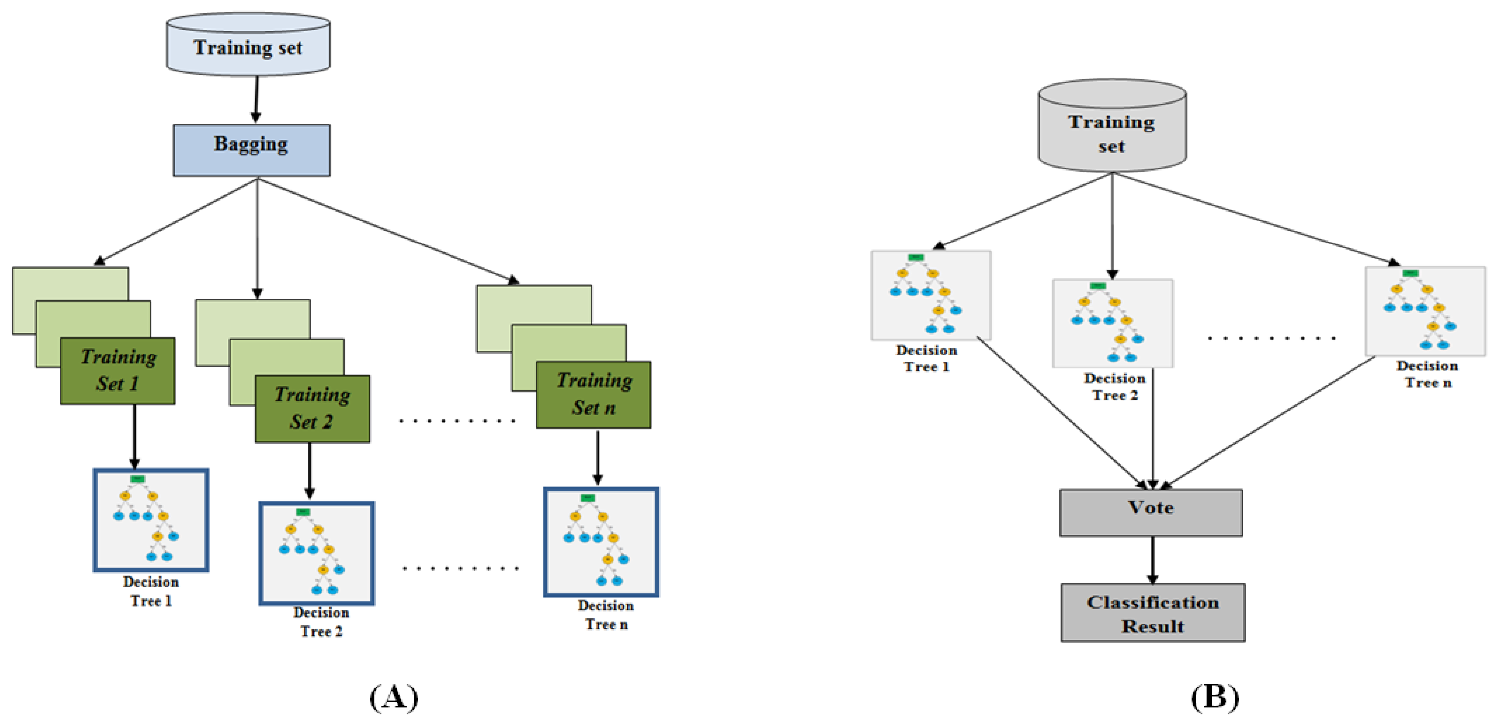
Figure 2.
Probability distributions of device categories predicted by a gradient-boosting.
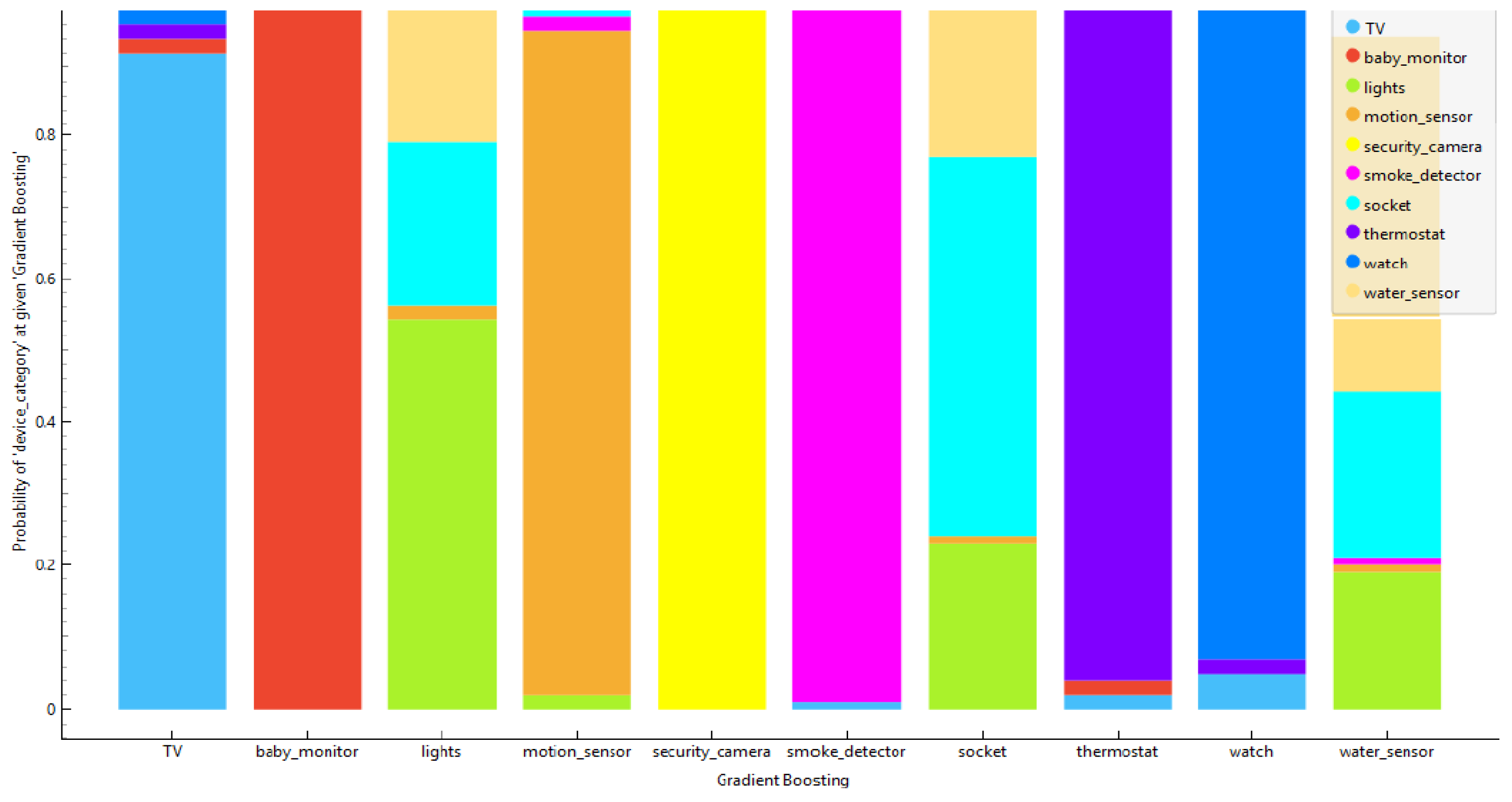
Figure 3.
Probability distributions of device categories predicted by Random Forest.
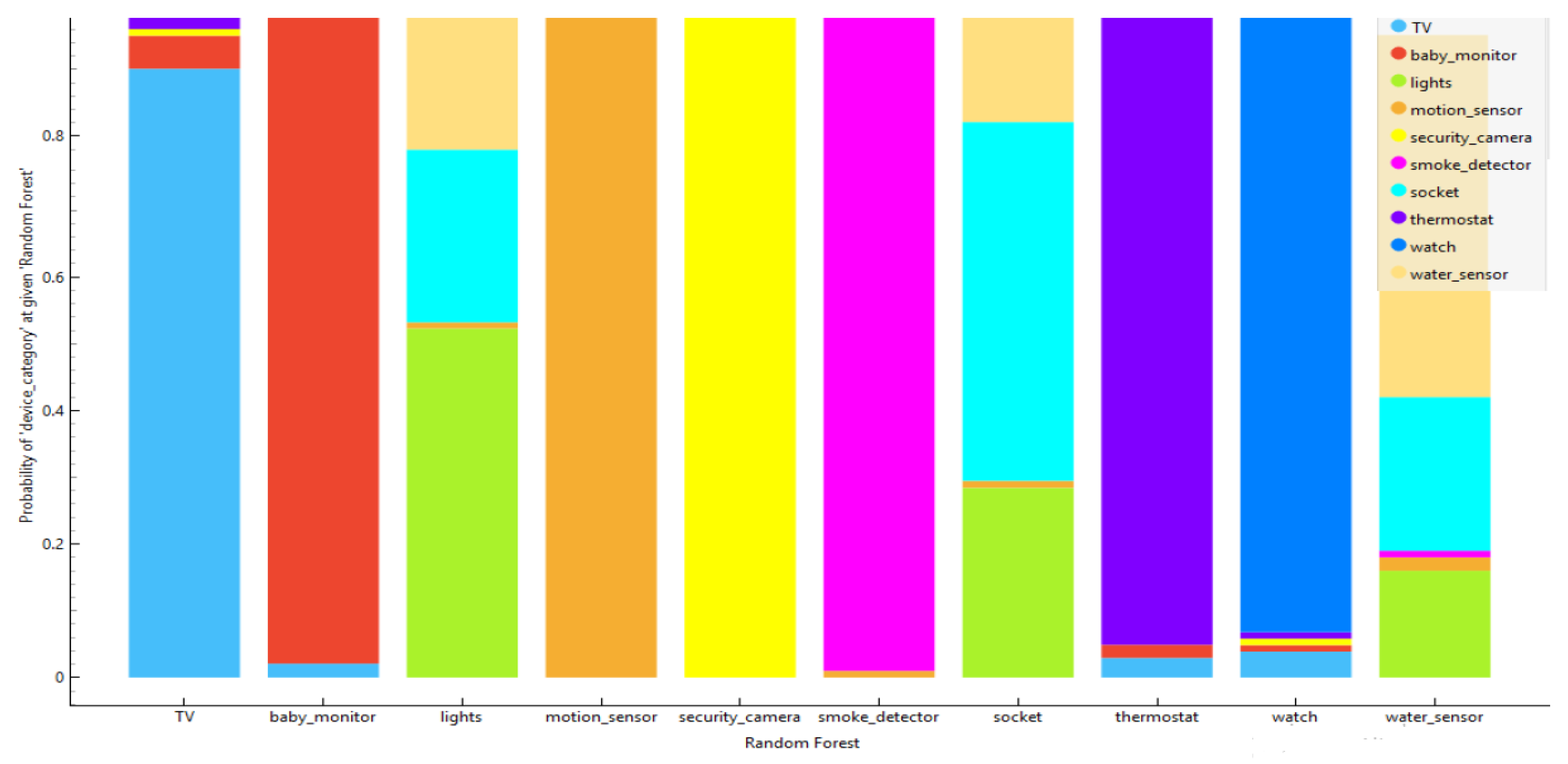
Figure 4.
Confusion Matrix for Gradient Boosting.
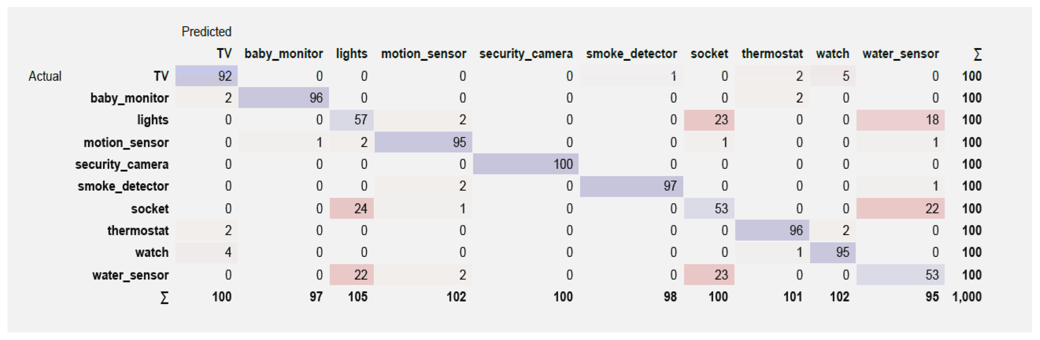
Figure 5.
Confusion Matrix for Random Forest.
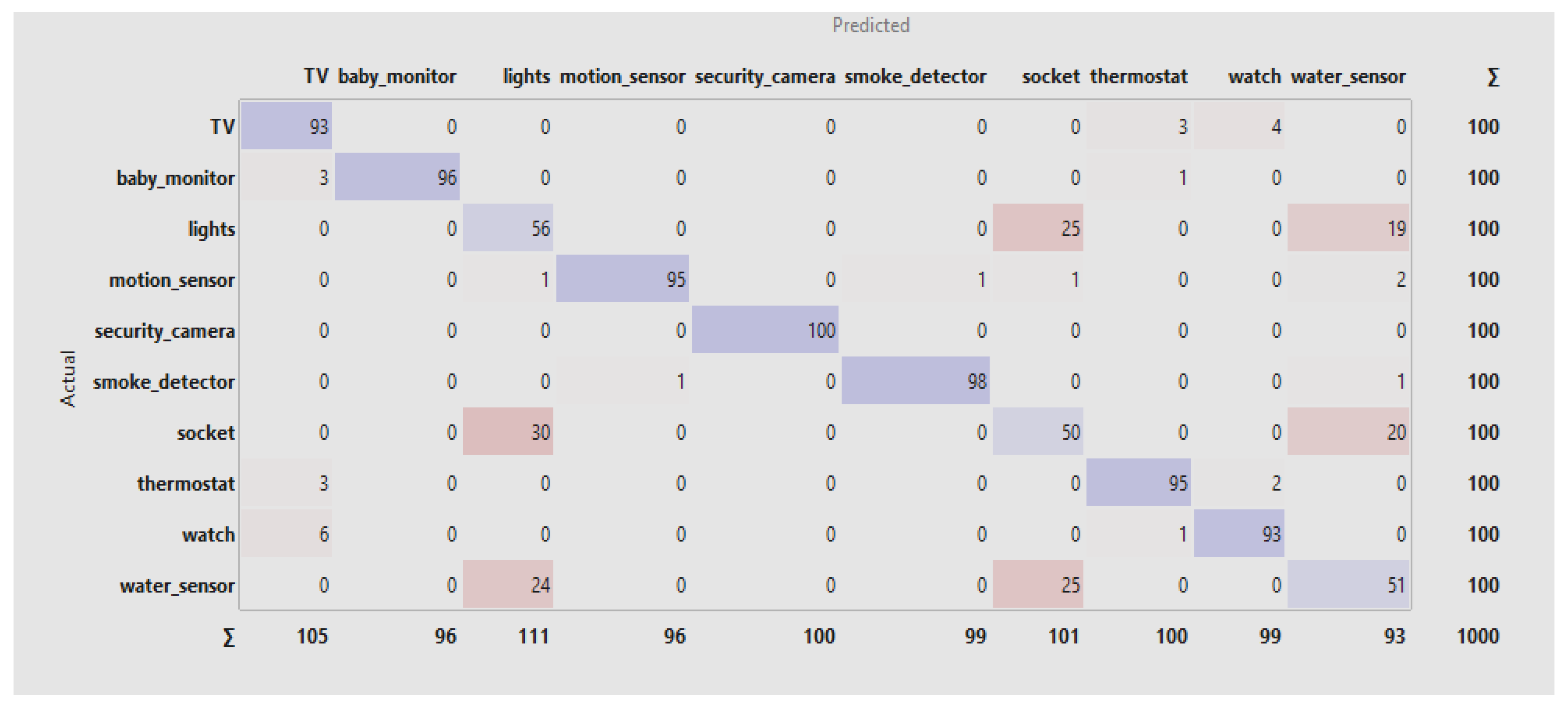
Figure 6.
ROC Curve Analysis for the Baby Monitor and TV Classes .
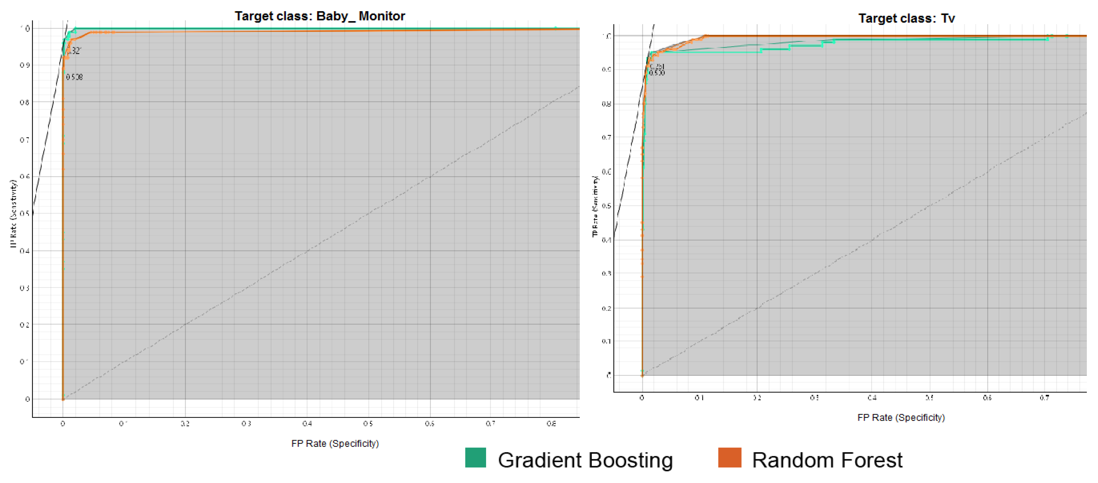
Figure 7.
ROC Curve Analysis for the Lights and Motion _Sensor Classes.
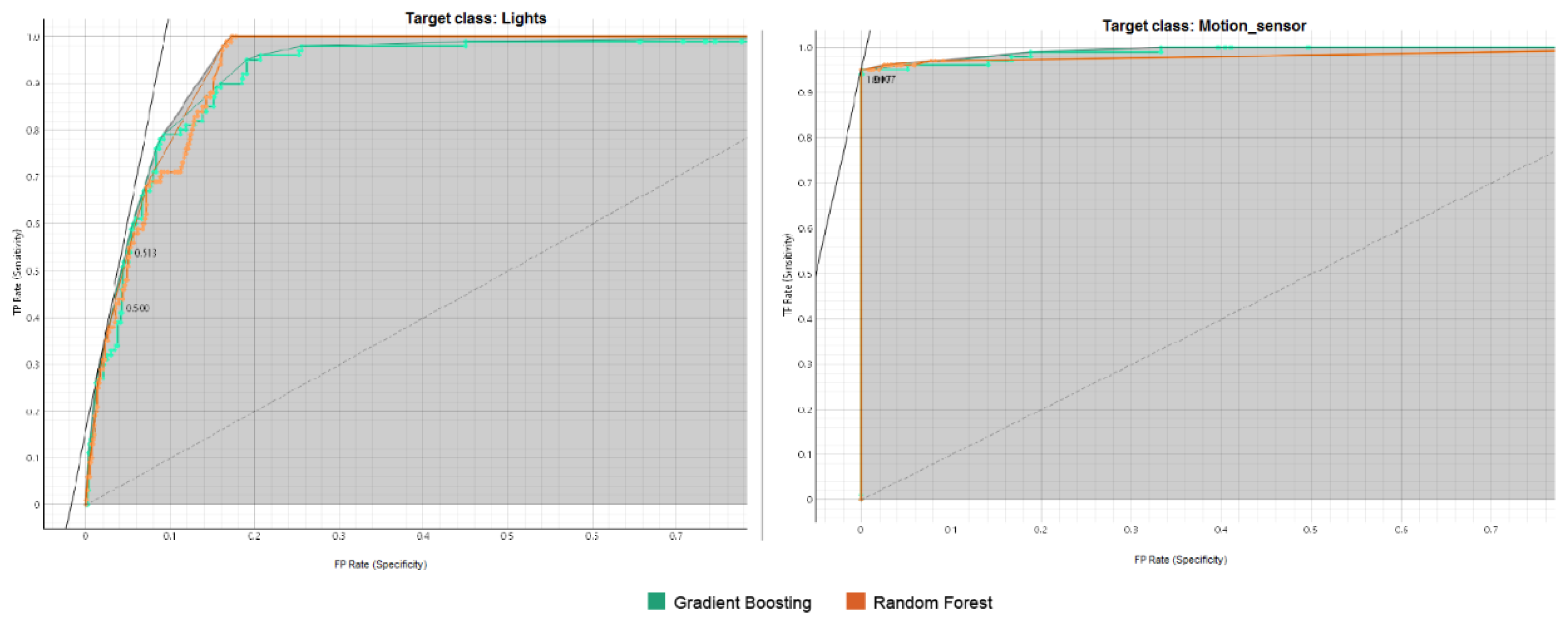
Figure 8.
ROC Curve Analysis for the Security Camera and Smoke_Detector Classes.

Figure 9.
ROC Curve Analysis for Socket and Thermostat Classes.
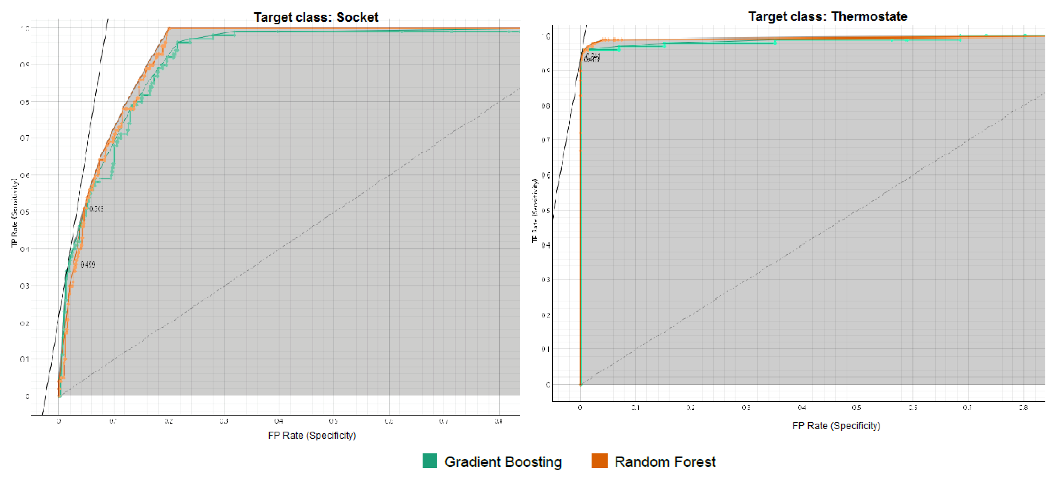
Figure 10.
ROC Curve Analysis for Watch and Water _Sensor Classes.
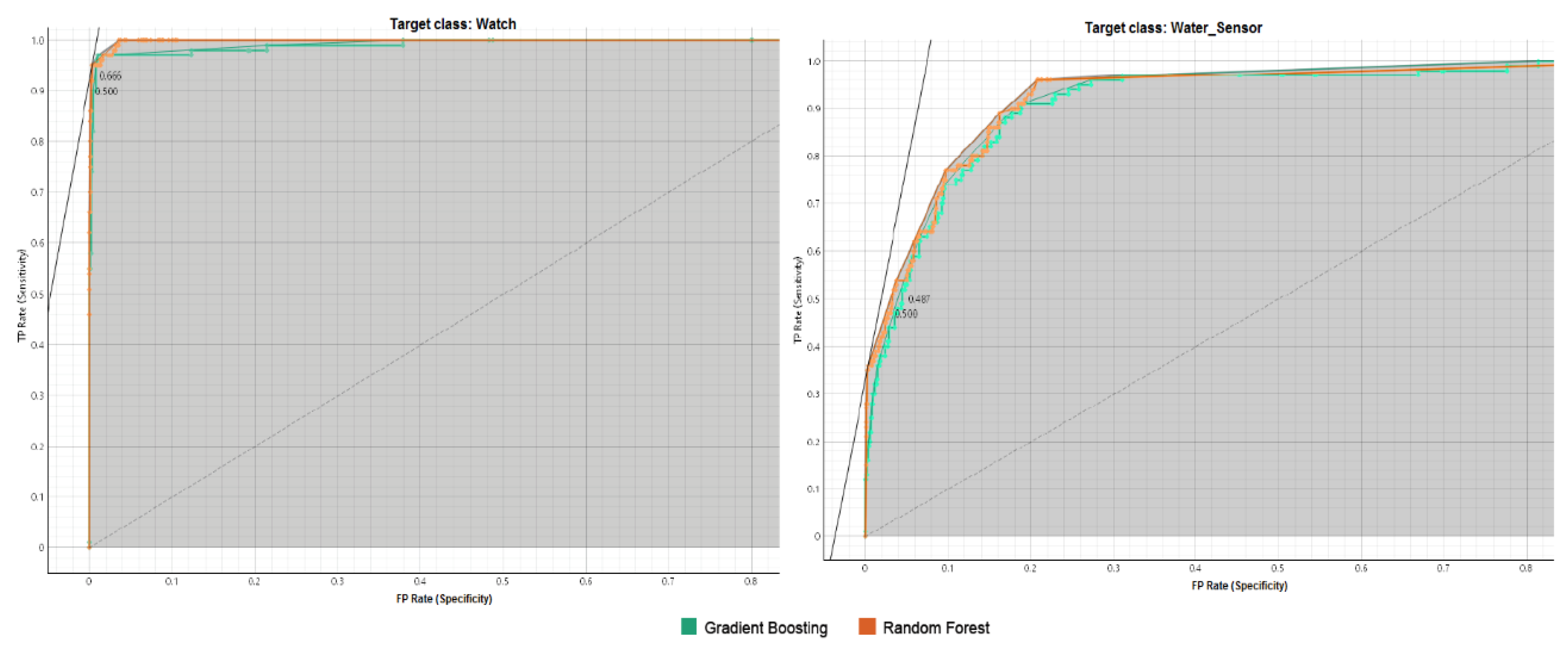

Table 1.
The performance metrics of Gradient Boosting for classifying various target classes.
| Gradient Boosting | Metrics Class | AUC | ACC | F1 | Precision | Recall | MCC |
| TV | 0.979 | 0.984 | 0.920 | 0.920 | 0.920 | 0.911 | |
| Baby monitor | 1.00 | 0.995 | 0.975 | 0.990 | 0.960 | 0.972 | |
| Lights | 0.926 | 0.909 | 0.556 | 0.543 | 0.570 | 0.506 | |
| Motion sensor | 0.991 | 0.988 | 0.941 | 0.931 | 0.950 | 0.934 | |
| Security camera | 1.00 | 1.00 | 1.00 | 1.00 | 1.00 | 1.00 | |
| Smoke detector | 0.997 | 0.996 | 0.980 | 0.990 | 0.970 | 0.978 | |
| socket | 0.920 | 0.906 | 0.530 | 0.530 | 0.530 | 0.478 | |
| Thermostat | 0.987 | 0.991 | 0.955 | 0.950 | 0.960 | 0.950 | |
| Watch | 0.991 | 0.988 | 0.941 | 0.931 | 0.950 | 0.927 | |
| Water sensor | 0.914 | 0.911 | 0.544 | 0.558 | 0.530 | 0.495 |
Table 2.
The performance metrics of Random Forest for classifying various target classes.
| Random Forest | Metrics Class | AUC | ACC | F1 | Precision | Recall | MCC |
| TV | 0.998 | 0.981 | 0.907 | 0.886 | 0.930 | 0.897 | |
| Baby monitor | 0.999 | 0.996 | 0.980 | 1.00 | 0.960 | 0.978 | |
| Lights | 0.936 | 0.901 | 0.500 | 0.505 | 0.560 | 0.475 | |
| Motion sensor | 0.984 | 0.994 | 0.960 | 0.990 | 0.950 | 0.966 | |
| Security camera | 1.00 | 1.00 | 1.00 | 1.00 | 1.00 | 1.00 | |
| Smoke detector | 0.995 | 0.997 | 0.985 | 0.990 | 0.980 | 0.983 | |
| socket | 0.912 | 0.899 | 0.498 | 0.495 | 0.500 | 0.441 | |
| Thermostat | 0.989 | 0.990 | 0.950 | 0.950 | 0.950 | 0.944 | |
| Watch | 0.999 | 0.987 | 0.935 | 0.939 | 0.930 | 0.927 | |
| Water sensor | 0.934 | 0.919 | 0.585 | 0.600 | 0.570 | 0.540 |
Table 3.
The overall performance matrices of Random Forest and Gradient Boosting Algorithms.
| Model | AUC | CA | F1 | Precision | Recall | MCC |
|---|---|---|---|---|---|---|
| Random Forest | 0.997 | 0.981 | 0.905 | 0.901 | 0.910 | 0.895 |
| Gradient Boosting | 0.979 | 0.984 | 0.920 | 0.920 | 0.920 | 0.911 |
Disclaimer/Publisher’s Note: The statements, opinions and data contained in all publications are solely those of the individual author(s) and contributor(s) and not of MDPI and/or the editor(s). MDPI and/or the editor(s) disclaim responsibility for any injury to people or property resulting from any ideas, methods, instructions or products referred to in the content. |
© 2025 by the authors. Licensee MDPI, Basel, Switzerland. This article is an open access article distributed under the terms and conditions of the Creative Commons Attribution (CC BY) license (http://creativecommons.org/licenses/by/4.0/).
Copyright: This open access article is published under a Creative Commons CC BY 4.0 license, which permit the free download, distribution, and reuse, provided that the author and preprint are cited in any reuse.


