
Submitted:
05 February 2025
Posted:
06 February 2025
You are already at the latest version
Abstract
Sparse Synthetic Aperture Radar (SAR) imaging has garnered significant attention due to its ability to suppress azimuth ambiguity in under-sampled conditions, making it particularly useful for high-resolution wide-swath (HRWS) SAR systems. Traditional compressed sensing -based sparse SAR imaging algorithms are hindered by range-azimuth coupling induced by range cell migration (RCM), which results in high computational cost and limits their applicability to large-scale imaging scenarios. To address this challenge, the approximated observation-based sparse SAR imaging algorithm was developed, which decouples the range and azimuth directions, significantly reducing computational and temporal complexities to match the performance of conventional matched filtering algorithms. However, this method requires iterative processing and manual adjustment of parameters. In this paper, we propose a novel deep neural network-based sparse SAR imaging method, namely Self-supervised Azimuth Ambiguity Suppression Network (SAAS-Net). Unlike traditional iterative algorithms, SAAS-Net directly learns the parameters from data, eliminating the need for manual tuning. This approach not only improves imaging quality but also accelerates the imaging process. Additionally, SAAS-Net retains the core advantage of sparse SAR imaging—azimuth ambiguity suppression in under-sampling conditions. The method introduces self-supervision to achieve orientation ambiguity suppression without altering the hardware architecture. Simulations and real data experiments using Gaofen-3 validate the effectiveness and superiority of the proposed approach.
Keywords:
azimuth ambiguity suppression
; SAR imaging
; unfolded imaging network
1. Introduction
High-resolution synthetic aperture radar (SAR) imaging algorithms have recently earned significant attention in the field of SAR imaging. However, due to the constraints imposed by the Nyquist Sampling Theorem, achieving high-resolution wide-format imaging needs higher sampling rates. The SAR imaging problem, viewed as an inverse problem, can potentially overcome this limitation through the application of compressed sensing theory[1,2]. The first proposed application of compressed sensing theory to SAR imaging algorithms was made by [3]. Subsequent work by [4,5,6] further enhanced sparse synthetic aperture radar algorithms. Additionally, compressed sensing algorithms have been applied in the fields of inverse synthetic aperture radar imaging [7,8] and three-dimensional imaging [9,10,11]. Compared to traditional SAR imaging methods, sparse SAR imaging algorithms can reduce the number of samples. However, most of these algorithms operate in the time domain, overlooking or failing to account for azimuth-distance coupling. As a result, they suffer from high computational complexity and memory usage, making them challenging to apply to large-scale scenes or wide-format imaging. [12] proposed an approximated observation-based sparse SAR imaging algorithm which can significantly reduce computational and temporal complexities. This approach maintains consistency in computational complexity and matched filtering algorithms.
In practice, traditional sparse synthetic aperture radar imaging algorithms often require manual parameter tuning. This means that the parameters must be readjusted for different imaging scenarios, and the entire tuning process is heavily reliant on manual experience. In recent years, SAR imaging based on deep learning has been widely used[13,14,15,16,17,18], leveraging deep learning for adaptive parameter adjustment. [19] introduced the concept of a sparse unfolding network by leveraging the properties of neural networks. This method replaces the iterative process of the original algorithm with a multi-layer neural network, which is used to automatically train and adjust the parameters that would traditionally need manual fine-tuning, ensuring that the parameters are selected optimally. In recent years, deep unfolding networks have found applications in sparse synthetic aperture radar imaging. In [20], a joint range migration and sparse reconstruction network for 3D millimeter-wave imaging was introduced. In [21,22], a SAR imaging framework based on the depth-expanded network of ISTA was proposed and successfully applied to passive SAR. However, these methods are limited in their ability to effectively utilize the structural information inherent in SAR signals, and therefore cannot address issues such as range ambiguity and azimuth ambiguity.
Since the energy of azimuth ambiguity cannot be ignored in practical applications, it is essential to pay attention to azimuth ambiguity suppression in sparse SAR imaging. Azimuth ambiguity suppression using filter combinations [23] is a commonly employed algorithm, which can be partially achieved by reducing spectral aliasing in the azimuth direction through filtering. However, this approach has certain limitations. For instance, it necessitates precise knowledge of the azimuth spectrum, and the extent of azimuth ambiguity suppression is limited. Additionally, implementing this technique often requires sacrificing a portion of the azimuth bandwidth. [24] proposed an iterative algorithm to reconstruct high-resolution images by using the original image as prior information and the truncated spectrum as the observation in each iteration. However, this algorithm suffers from high computational complexity and low efficiency, making it challenging to apply in large-scale scenes. Additionally, the iterative process requires manual parameter tuning, which means the imaging results are highly sensitive to factors such as user experience, and the algorithm’s adaptability to different scenes is quite limited. [25,26] proposed an orientation ambiguity suppression algorithm based on group sparsity, which can partially suppress ambiguity in the orientation direction. However, this method requires manual parameter adjustment and involves a large computational workload, leading to high computational cost. As a result, it is difficult to apply in fast imaging scenarios. [27] proposed using a reconstruction filter to accurately reconstruct azimuthal ambiguity and then suppress it. However, this method is only effective for suppressing azimuthal ambiguity in small areas and for small targets. [28] proposed an estimation algorithm based on the minimum mean square error, using a subspace algorithm for ambiguity suppression. However, this method involves a large computational workload, making it difficult to apply in the imaging process of large scenes. [29] proposed an algorithm that uses the weighted energy of regions less affected by ambiguityring to perform extrapolation and obtain the full spectrum. However, this algorithm introduces noise, leading to imaging quality that is lower than desired.
Existing ambiguity suppression algorithms can be broadly categorized into three types: directly or indirectly utilize the filtering results of filters, sparse reconstruction-based algorithms, and use regions with less ambiguity for imaging. Whether the filter results are directly applied to imaging or used as part of the a priori knowledge, precise knowledge of the spectrum is essential. While filtering can suppress spectral aliasing in certain regions, it often negatively affects the spectrum in the main region as well. Sparse reconstruction-based approaches typically involve large-scale computations with high complexity. These methods often require manual parameterization, making the results highly sensitive to human input and resulting in poor adaptability. Due to the imaging characteristics of radar systems, it is difficult to identify regions with minimal ambiguity. As a result, the practical application of algorithms that rely on imaging regions with less ambiguity faces significant challenges.
Based on this, in this paper, we investigate the cause of azimuthal ambiguity and introduce group sparse constraints to reformulate the SAR imaging model. We employ the compressed sensing algorithm for sparse reconstruction and leverage a network structure to train the parameters that would typically require manual adjustment, significantly mitigating the issue of insufficiently accurate manual tuning. Additionally, a self-supervised algorithm is introduced to address the problem of traditional neural network-based imaging algorithms being overly dependent on existing datasets. The entire algorithm is built upon the chirp scaling algorithm. This choice is motivated by the fact that, under the assumption of a small oblique viewing angle, the chirp scaling algorithm can perform range migration correction more accurately through phase multiplication, rather than interpolation. This is in contrast to the distance Doppler algorithm, which relies on interpolation to handle range migration in the distance-time-azimuth-frequency domain (distance Doppler domain). While the Omega-K algorithm can provide more precise results, it demands more computational resources and is not suitable for large-scale scene imaging.
The main contributions of the article are as follows:
1)Sparse Expansion of the Iterative Process: The iterative process of traditional algorithms is sparsely expanded, and a deep unfolded network is introduced for adaptive training of parameters. This approach addresses the challenges of large computational load, slow processing speed, and poor generalization inherent in traditional algorithms.
2)Self-Supervised Imaging Network: A self-supervised imaging network structure is designed to tackle the problem of insufficient datasets. This network eliminates the need for manual parameter adjustments and enhances the network’s adaptability to different imaging scenes.
3)Structural Sparsity for Azimuthal Ambiguity Suppression: The concept of structural sparsity is introduced, and the lq-norm is applied for azimuthal ambiguity suppression, leading to further improvements in imaging quality. Joint Loss Function: A joint loss function, combining structural sparsity and principal view clarity, is formulated to achieve azimuthal ambiguity suppression while maintaining robustness against noise.
This method is evaluated using both simulated point targets and real-world datasets. The experimental results highlight the effectiveness of the algorithm in reducing sidelobes and enhancing target features, demonstrating its potential for tackling challenges in large-scale imaging scenarios.
The rest of this article is organized as follows. Section II presents the SAR signal model including the sparse SAR imaging model and the azimuth ambiguity signal model. Section III describes the structure of the basic imaging model as well as the structure of proposed model and provides details on the SAAS-Net. In Section IV, both simulation experiments and real data experiments are presented. Finally, the conclusion are drawn in Section V.
2. Signal Model
2.1. Sparse SAR Imaging Model
The sparsity of a signal refers to the presence of many components that are nearly zero in some representation. In such cases, signal reconstruction can be achieved at a sampling rate much lower than that dictated by the Nyquist sampling theorem, using techniques like compressed sensing. Given represents the scattering coefficient of the observation scene, represents the echo signal, represents the observation matrix, n represents the noise signal and the imaging model of sparse SAR can be expressed as:
Essentially, the sparse SAR imaging process is a classic inverse problem which can be solved by compressed sensing methods. Within the compressed sensing framework, the sparse SAR imaging problem can be rewritten as a regularized expression:
Where is a regularization parameter that determined by the sparsity of the imaging scene.
As a convex relaxation, the -norm optimization problem can be approximated by a -norm optimization as follows:
As for this optimization problem with the form of least absolute shrinkage and selection operator(LASSO), it can be solved by the Iterative Shrinkage-Thresholding Algorithm(ISTA). In this optimization system, the parameter is always determined by artificial setting based on the sparsity of the imaging scene and the iterative expression is:
Where and are regularization parameters, is the scattering coefficient of the observation scene, is the echo signal, is the observation matrix.
2.2. Azimuth Ambiguity Suppression Signal Model
Sampling in the azimuth direction tends to be non-uniform compared to the range direction, making it more prone to undersampling at certain beam locations. This non-uniform sampling can lead to spectral aliasing in the azimuth direction, resulting in azimuth ambiguity. Since the azimuth PRF and the image width are interdependent, improving azimuth resolution and mapping width simultaneously is not feasible. Therefore, to achieve high-resolution wide-area imaging, it is crucial to explore techniques for mitigating azimuth ambiguity. Specifically, for the Gaofen-3 system, the azimuth pulse repetition frequency (PRF) is slightly lower than the minimum PRF required for uniform sampling at certain beam positions, leading to azimuth undersampling and, consequently, azimuth ambiguity in the resulting images.
During sparse SAR imaging, the portion of the doppler spectrum that exceeds the PRF is folded into the azimuth processing bandwidth, causing it to mix with the main signal and resulting in azimuth ambiguity. As shown in Figure 1, the green and red dotted lines illustrate how the ambiguity areas fold into the main area. That is to say that the finite number of samples in the azimuth direction leads to spectral aliasing in the azimuth direction, resulting in the azimuth ambiguity. The structure of the SAR imaging operator in the ambiguous regions closely resembles that in the main area, except the azimuth frequency. Which means we can use different scattering coefficients to represent signals from different parts. If each set of data is considered as echo data from different angles, then the entire signal model can be expressed as follows:
Where represents the signal echo as the sparse imaging model. represents the image data from different angles, when the , the signal model is the same as the traditional signal model, which means when , the signal can be seen as the primary view. Further, other parts can be seen as expanded view. is the observation matrix.
Although the phase and amplitude of the primary and expanded view components of the target may be different, they are always at the same location in the scene, and thus group sparsity can be utilized to portray this sparsity. Introducing the group sparsity constraint. The optimization problem, when constrained by both group sparse constraints and -norm constraints, can be formulated as follows:
Just as the basic signal model, this optimization problem can be approximated by a -norm optimization:
Where represents the group sparsity constraint when indicates signal weights and . The regularization contains two constraint terms, the first one is the group sparsity constraint, and another is the enhancement of the penalty term for subjective sparsity for suppressing residual ambiguity energy. And according to [12], it can also be solved by the ISTA as the basic signal model.
3. The Structure of the Imaging Network
3.1. The Structure of Basic ISTA Network
If we use I to denote the imaging process of the chirp-scaling(CS) algorithm. Obviously, each step of CS imaging process is a one-dimensional linear algorithm, so the whole process of CS imaging can be regarded as a series of combinations of one-dimensional steps which can be expressed by the following expression:
In which, represents the FFT operation on azimuth direction, represents the FFT operation on range direction, represents the IFFT operation on azimuth direction, represents the IFFT operation on range direction. represents the range cell migration correction (RCMC) phase term, represents the range compression phase term, represents the azimuth-range decoupling phase term.
Thereby there is a similar form of CS imaging inverse process expression, in which G represents the inverse algorithm of the imaging process which is called echo simulation operator. The structure of the I and G operators are shown in Figure 2, and the G can be expressed as follows:
Since each step in the imaging process is a one-dimensional linear algorithm, every imaging step can be represented by matrix multiplication. In other words, the entire imaging process can be expressed as a series of matrix multiplications. If matrix and are used to represent the product of these matrices, then the imaging result and the echo signal should satisfy the following relationship:
At this point the relationship between the echo signal and the imaging is successfully established through the sparse observation matrix. As a convex optimization problem, it can be solved by the Iterative Shrinkage-Thresholding Algorithm(ISTA) and the iterative formula is as follows:
Where and are the regularization parameters, is the scattering coefficient of the observation scene, is the echo signal, is the inverse algorithm matrix of the imaging process and is the algorithm matrix of the imaging process.
It is obvious that the two parameters: step size and threshold need to be manually adjusted, and the results of these parameters have a great impact on the experimental results. Therefore, it is considered to utilize the design of a network structure to train these two parameters, which ensures that these two parameters are unified in each layer and adaptively get trained between different layers of the network. And the structure of the ISTA-Net is shown in Figure 3.
3.2. The Structure of Azimuth Ambiguity Suppression Network
In practice, undersampling in the azimuthal direction often results in ambiguous energy, leading to azimuthal ambiguity. To address this issue, we introduce group sparsity.
The ambiguity component in the azimuthal direction can be considered as another signal with different observation angles. As a result, the overall signal model at this point can be viewed as a superposition of the ambiguity component and the dominant visual component. In this case, the ambiguity component and the dominant visual component have the same energy distribution, meaning that both the ambiguity solution and the non-ambiguity solution will appear at the same position in the sparse SAR imaging process, with the only difference being the amplitudes of the signals. Therefore, group sparsity can be used to characterize the relationship between the ambiguity and non-ambiguity solutions. At this stage, the number of ambiguous solutions corresponds to the number of ghost images, while the number of non-ambiguous solutions matches the group sparsity. This sparsity is crucial for suppressing azimuthal ambiguity.
According to the formula (6) in signal model section, if , then the azimuth ambiguity suppression regularization problem mentioned before can be rewritten as a typical sparse regularization problem:
| Algorithm 1: algorithm of azimuth ambiguity based sparse imaging |
|
It is obvious that this is a convex problem, and we can use the fast Iterative Shrinkage Thresholding Algorithm(FISTA) to solve this problem. Given the , we can use algorithm 1 to depict this process.
The represents the residual, U represents gradient direction, t is the FISTA iteration parameters, is the image signal and is the intermediate variable of FISTA algorithm, and are manually adjust parameters. Similar to the basic network, we can use a deep unfolded network to train these parameters, and the structure of the unfolded network is shown in Figure 4. For ease of representation, we divide the entire network structure into four modules,, , , and , which are used to update the parameter t, the principal view , the gradient , and the intermediate variable .
3.3. The Training Process of the Azimuth Ambiguity Suppression Network
In practical applications, there is often an insufficient amount of data to support the training process. Additionally, different imaging scenes typically exhibit varying levels of scene sparsity, which requires adjusting iteration parameters accordingly. Therefore, it is essential to design self-supervised imaging networks to address these challenges.
As shown in Figure 5, we design an encoder-decoder network to enable the self-supervised operation of the entire unfolding network. In the encoder, the raw echo signal is partitioned into L smaller echoes. Three of these raw echoes are randomly selected to generate the corresponding reference imaging results, which serve as labels for training the network. The network model is trained using these three sets of reference echoes and their corresponding reference imaging results. In the decoder, the partitioned raw echo signals are processed through the encoder-trained network model to obtain small-area imaging results for each chunk. These imaging results are then stitched together to form the complete large-area imaging output from the decoder. It is noteworthy that within the decoder section, a branch connection is incorporated. This connection directly feeds the echo signal from the encoder input segment into the decoder input, ensuring the seamless progression of the imaging process.
The loss function of this network consists of a composite regularization term:
In which is main view regularization, and is group sparsity regularization, is regulation parameter. The whole loss function is a linear combination of the main view regularization and group sparsity regularization, by using this joint loss function, azimuth ambiguity can be effectively suppressed.
4. Experiments
In this chapter, we analyze the performance of the proposed imaging net on point targets imaging experiments. Since the proposed imaging network is formed by sparse SAR imaging based on ISTA with chirp-scaling operator, we compare our network with the sparse imaging algorithm based on the chirp-scaling algorithm, and the unfolded network based on the chirp-scaling imaging algorithm as well as the traditional SAR imaging algorithm which has the azimuth ambiguity suppression operation. For the convenience of presentation, we denote the sparse imaging algorithm based on chirp-scaling as CS-IST algorithm, the traditional azimuth ambiguity suppression algorithm as CS-IST-AAS, the unfolded network based on the chirp-scaling imaging algorithm as ISTA- Net, the unfolded network based on self-supervised azimuth ambiguity suppression as AAS-Net, the self-supervised imaging network as SAAS-Net.
4.1. Simulation Experiments
4.1.1. Point Target Imaging Experiment
We designed a point-target simulation experiment to test the effectiveness of the network proposed in this paper in terms of orientation ambiguity suppression. The parameters of the simulation experiment are shown in the Table 1. We used the CS-IST algorithm, ISTA-Net, CS-IST-AAS algorithm, and AAS-Net for point target imaging at 60% undersampling, and the imaging results are shown in Figure 6.
The Figure 6 shows one of the point targets imaging results of CS-IST, CS-IST-SSA, ISTA-Net and AAS-Net. The radar parameters and the echo generation of the point targets are the same which are shown in Table 1. In the imaging results, the longitudinal direction is the azimuthal direction and the transverse direction is the range direction. In contrast, the ISTA-Net algorithm in Figure 6(b) can weaken the azimuth ambiguity to a certain degree because of the introduction of the network. And the ambiguity phenomenon is eliminated in Figure 6(c) and (d). It indicates that the proposed azimuth ambiguity suppression algorithm can significantly reduce the sidelobes which leads to the more accurate reconstruct results. And the proposed network has better azimuth ambiguity suppression capabilities. For quantitative comparing, a Monte Carlo experiment was conducted, and PSNR, ISLR and mean AASR along azimuth detection to evaluate the imaging quality are used to evaluate the imaging quality, and the results are shown in Table 2.
Monte Carlo experiments further demonstrate the effectiveness of the ambiguity suppression algorithm proposed in this paper for azimuthal ambiguity suppression. In addition, utilizing the unfolding network training, the imaging quality is higher than that of the traditional algorithm because better iteration parameters can be obtained.
To better show the imaging effectiveness of the algorithms,
we located the point of maximum value and conducted interpolation by 16 times, and the interpolated azimuthal slice is shown in Figure 7. It indicates that the algorithm in Figure 7(d) can significantly reduce the sidelobes, which indicates the proposed network is more effective in suppressing the azimuth ambiguity due to the adaptive threshold parameter setting.
The azimuthal results show that the azimuthal sidelobe of the algorithm proposed in this paper is significantly reduced and thus has the best azimuthal ambiguityring suppression.CS-IST-AAS also has some effect on ambiguityring suppression. The CS-IST and ISTA-Net algorithms, on the other hand, do not perform additional sparse optimization of the azimuthal direction and thus suffer from spectral aliasing in the azimuthal direction when the azimuthal direction is undersampled. In the process of gradually reducing the sampling rate, the algorithm in this paper is relatively less affected, and the side flap suppression effect is relatively good. In the experiment added 30db of Gaussian noise, this paper’s algorithm can still be good for ambiguity suppression, and it can be seen that this paper’s algorithm has a certain degree of noise robustness.
4.1.2. Point Target Undersampling Imaging Experiment
To show the effectiveness of the sampling pattern generated by our proposed network, we have selected the same scene under 30% undersampling, 70% undersampling and 90% undersampling and calculated the AASR at this point. The results of the experiments are shown in the Table 3, in order to further demonstrate the superiority of this paper’s algorithm in azimuthal ambiguity suppression
4.2. Real Data Experiments
4.2.1. Real Data Imaging Experiment
We used the data from Gaofen-3 system to conduct the imaging experiment of the actual data. We used four algorithms, CS-IST, CS-IST-AAS, ISTA-Net and proposed method, respectively, to image the actual data, and their imaging results are shown in Figure 8. There are two target ships in the imaging scene. It can be observed that due to undersampling in the azimuth direction, both the conventional CS-IST algorithm and the ISTA-Net algorithm suffer from severe azimuth ambiguity, with artifacts appearing above or below the target ship. The presence of artifacts in the imaging scene is almost invisible in the imaging results using proposed method as well as the CS-IST-AAS algorithm. The imaging quality of the algorithm proposed and CS-IST-AAS is basically suppressed. In order to further compare the imaging results of those algorithms, the AASR and computing time of these four algorithms are compared, and the results are shown in the Table 4. It can be seen that the ambiguity suppression effect of proposed algorithm in the azimuthal direction is not much different from that of the CS-IST-AAS algorithm, and at the same time, the imaging speed is much higher than that of the CS-IST-AAS algorithm.
In order to quantitatively compare the imaging quality of these algorithms, we calculated their AASR, and at the same time, we also compared the imaging speed of these algorithms, and the results are shown in the following table. The algorithm in this paper has comparable ambiguity suppression effect with CS-IST-AAS algorithm, and the computational speed is improved about 800 times than CS-IST-AAS algorithm. Therefore, the algorithm in this paper can realize fast imaging with azimuthal ambiguity suppression.
We have sliced the azimuthal direction of the real data, and it can be seen that the azimuthal sidelobes are significantly reduced in the algorithm of this paper and CS-IST-AAS, and the other two algorithms have significant ambiguity energy in the azimuthal direction.
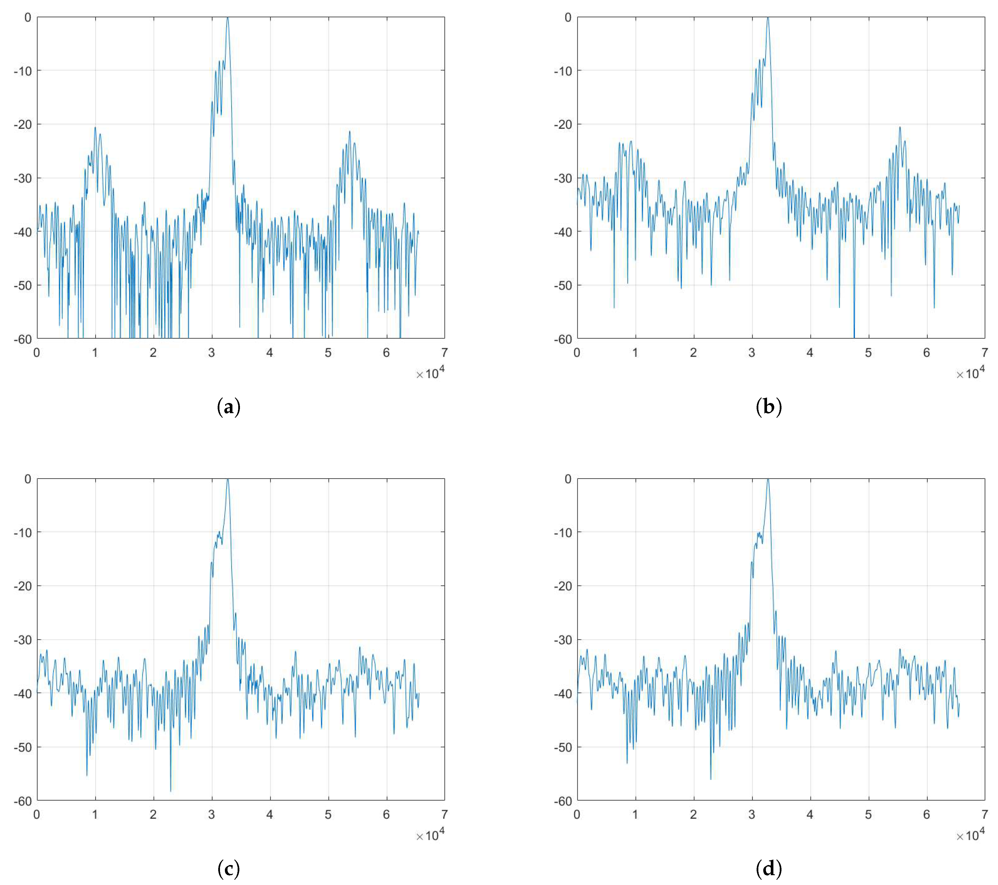
Figure 9.
Azimuth frequency spectrum: (a) The sparse imaging algorithm based on chirp-scaling. (b) The unfolded network based on the chirp-scaling imaging algorithm. (c) The traditional azimuth ambiguity suppression algorithm based on group sparsity. (d) Proposed method.
Figure 9.
Azimuth frequency spectrum: (a) The sparse imaging algorithm based on chirp-scaling. (b) The unfolded network based on the chirp-scaling imaging algorithm. (c) The traditional azimuth ambiguity suppression algorithm based on group sparsity. (d) Proposed method.
4.2.2. Real Data Undersampling Image Experiment
In this section, we conducted comparative experiments using ISTA-net and the proposed network at downsampling rates of 80%, 60%, and 30% , adding 20dB of noise throughout the experiment. The results are presented in Figure 10.
There are three ships can be seen in Figure 10(a). In fact, the center portion represents the actual ship imaged, while the ships above and below are artifacts due to azimuthal ambiguity. At a downsampling rate of 80%, artifacts in the upper and lower vessels due to orientation ambiguity are visible with ISTA-net, while these ambiguity artifacts are barely noticeable in the proposed network. At a downsampling rate of 60%, the artifacts in ISTA-net become more prominent, and a slight artifact also appears in the proposed network. At a downsampling rate of 30%, both algorithms exhibit clear artifacts, but the ambiguity energy in the proposed network remains significantly lower than that in ISTA-net, demonstrating the effectiveness of the proposed algorithm in suppressing ambiguity energy in the azimuth direction. This demonstrates that the algorithm presented in this paper effectively suppresses ambiguity energy in the azimuth direction.At the same time, the algorithm in this paper is robust to noise.
4.2.3. Network Iteration Layer Experiment
In order to further demonstrate the structural properties of the network, we show the results for each layer of the imaging process in Figure 11, and it can be seen that when the number of iterative layers is 1, the outline of the imaging gradually appears, but it still has a lot azimuth ambiguity. With the increase of the number of iterative layers, the imaging quality gradually improves until it reaches the highest quality after the number of iterative layers is 5, after which the change is no longer obvious. As a result, the network essentially reaches convergence by the fifth layer, and with the overall network structure being relatively shallow, the training process can be completed quickly, thereby further enhancing imaging efficiency. Meanwhile, 20 dB of Gaussian noise is added in this experiment, and the imaging results are still clear, which also proves the robustness of the proposed algorithm.
5. Conclusions
Azimuth ambiguity can deteriorate SAR image quality and influence normal SAR applications. Limited by the azimuth sampling rate, azimuth ambiguity often occurs in sparse SAR imaging. In this article, we propose a novel sparse SAR imaging unfolded network which can help with azimuth ambiguity suppression. We design an encoder-decoder structure. The encoder generates reference imaging results and facilitates a self-supervised training process, while the decoder is responsible for the imaging procedure. Parameters are optimized through end-to-end training, allowing them to adaptively adjust without complex tuning. SAAS-Net learns the parameters directly from the data, eliminating the need for manual adjustment. This approach not only enhances the quality of imaging but also speeds up the entire process. Moreover, SAAS-Net preserves the key benefit of sparse SAR imaging—suppressing azimuth ambiguity under under-sampling conditions. The imaging experiments were conducted on both simulated datasets and real datasets to verify the efficiency of the algorithm proposed in this article and its effectiveness in suppressing azimuth ambiguity.
Author Contributions
Zhiyi Jin: Conceptualization; methodology; validation; writing—original draft; writing—review and editing. Zhouhao Pan: Conceptualization; supervision; writing— review and editing. Zhe Zhang: Funding; conceptualization; supervision; writing—review and editing. Xiaolan Qiu: Conceptualization; resources; supervision; writing— review and editing.
Conflicts of Interest
The authors declare no conflicts of interest.
Abbreviations
The following abbreviations are used in this manuscript:
| HRWS | high-resolution wide-swath |
| SAR | synthetic aperture radar |
| RCM | range cell migration |
| SAAS-Net | Self-supervised Azimuth Ambiguity Suppression Network |
| CS | chirp-scaling |
| PRF | pulse repetition frequency |
| ISTA | iterative shrinkage thresholding algorithm |
| FISTA | fast iterative shrinkage thresholding algorithm |
References
- Baraniuk, R.G. Compressive sensing [lecture notes]. IEEE signal processing magazine 2007, 24, 118–121. [Google Scholar] [CrossRef]
- Candès, E.J.; Romberg, J.; Tao, T. Robust uncertainty principles: Exact signal reconstruction from highly incomplete frequency information. IEEE Transactions on information theory 2006, 52, 489–509. [Google Scholar] [CrossRef]
- Patel, V.M.; Easley, G.R.; Healy, D.M.; Chellappa, R. Compressed synthetic aperture radar. IEEE Journal of selected topics in signal processing 2010, 4, 244–254. [Google Scholar] [CrossRef]
- Dong, X.; Zhang, Y. SAR image reconstruction from undersampled raw data using maximum a posteriori estimation. IEEE Journal of Selected Topics in Applied Earth Observations and Remote Sensing 2014, 8, 1651–1664. [Google Scholar] [CrossRef]
- Yang, D.; Liao, G.; Zhu, S.; Yang, X.; Zhang, X. SAR imaging with undersampled data via matrix completion. IEEE Geoscience and Remote Sensing Letters 2014, 11, 1539–1543. [Google Scholar] [CrossRef]
- Zeng, J.; Fang, J.; Xu, Z. Sparse SAR imaging based on L 1/2 regularization. Science China Information Sciences 2012, 55, 1755–1775. [Google Scholar] [CrossRef]
- Du, X.; Duan, C.; Hu, W. Sparse representation based autofocusing technique for ISAR images. IEEE Transactions on Geoscience and Remote Sensing 2012, 51, 1826–1835. [Google Scholar] [CrossRef]
- Zhang, L.; Xing, M.; Qiu, C.W.; Li, J.; Bao, Z. Achieving higher resolution ISAR imaging with limited pulses via compressed sampling. IEEE Geoscience and Remote Sensing Letters 2009, 6, 567–571. [Google Scholar] [CrossRef]
- Aguilera, E.; Nannini, M.; Reigber, A. A data-adaptive compressed sensing approach to polarimetric SAR tomography of forested areas. IEEE Geoscience and Remote Sensing Letters 2012, 10, 543–547. [Google Scholar] [CrossRef]
- Austin, C.D.; Ertin, E.; Moses, R.L. Sparse signal methods for 3-D radar imaging. IEEE Journal of Selected Topics in Signal Processing 2010, 5, 408–423. [Google Scholar] [CrossRef]
- Budillon, A.; Ferraioli, G.; Schirinzi, G. Localization performance of multiple scatterers in compressive sampling SAR tomography: Results on COSMO-SkyMed data. IEEE Journal of Selected Topics in Applied Earth Observations and Remote Sensing 2014, 7, 2902–2910. [Google Scholar] [CrossRef]
- Fang, J.; Xu, Z.; Zhang, B.; Hong, W.; Wu, Y. Fast compressed sensing SAR imaging based on approximated observation. IEEE Journal of Selected Topics in Applied Earth Observations and Remote Sensing 2013, 7, 352–363. [Google Scholar] [CrossRef]
- Wu, Y.; Zhang, Z.; Qiu, X.; Zhao, Y.; Yu, W. MF-JMoDL-Net: A Sparse SAR Imaging Network for Undersampling Pattern Design towards Suppressed Azimuth Ambiguity. IEEE Transactions on Geoscience and Remote Sensing 2024. [Google Scholar] [CrossRef]
- Mason, E.; Yonel, B.; Yazici, B. Deep learning for SAR image formation. In Proceedings of the Algorithms for Synthetic Aperture Radar Imagery XXIV. SPIE, Vol. 10201; 2017; pp. 11–21. [Google Scholar]
- Pu, W. Deep SAR imaging and motion compensation. IEEE Transactions on Image Processing 2021, 30, 2232–2247. [Google Scholar] [CrossRef] [PubMed]
- Zhao, S.; Ni, J.; Liang, J.; Xiong, S.; Luo, Y. End-to-end SAR deep learning imaging method based on sparse optimization. Remote Sensing 2021, 13, 4429. [Google Scholar] [CrossRef]
- Li, M.; Wu, J.; Huo, W.; Jiang, R.; Li, Z.; Yang, J.; Li, H. Target-oriented SAR imaging for SCR improvement via deep MF-ADMM-Net. IEEE Transactions on Geoscience and Remote Sensing 2022, 60, 1–14. [Google Scholar] [CrossRef]
- Li, M.; Wu, J.; Huo, W.; Jiang, R.; Li, Z.; Yang, J.; Li, H. Target-oriented SAR imaging for SCR improvement via deep MF-ADMM-Net. IEEE Transactions on Geoscience and Remote Sensing 2022, 60, 1–14. [Google Scholar] [CrossRef]
- Gregor, K.; LeCun, Y. Learning fast approximations of sparse coding. In Proceedings of the Proceedings of the 27th international conference on international conference on machine learning, 2010, pp.
- Wang, M.; Wei, S.; Liang, J.; Zeng, X.; Wang, C.; Shi, J.; Zhang, X. RMIST-Net: Joint range migration and sparse reconstruction network for 3-D mmW imaging. IEEE Transactions on Geoscience and Remote Sensing 2021, 60, 1–17. [Google Scholar] [CrossRef]
- Mason, E.; Yonel, B.; Yazici, B. Deep learning for SAR image formation. In Proceedings of the Algorithms for Synthetic Aperture Radar Imagery XXIV. SPIE, Vol. 10201; 2017; pp. 11–21. [Google Scholar]
- Yonel, B.; Mason, E.; Yazıcı, B. Deep learning for passive synthetic aperture radar. IEEE Journal of Selected Topics in Signal Processing 2017, 12, 90–103. [Google Scholar] [CrossRef]
- Moreira, A. Suppressing the azimuth ambiguities in synthetic aperture radar images. IEEE Transactions on Geoscience and Remote Sensing 1993, 31, 885–895. [Google Scholar] [CrossRef]
- Peng, X.; Youming, W.; Ze, Y.; et al. A SAR image azimuth ambiguity suppression method based on compressed sensing restoration algorithm. J. Radar 2016, 5, 39–45. [Google Scholar]
- Bingchen, Z.; Chenglong, J.; Zhe, Z.; Jian, F.; Yao, Z.; Wen, H.; Yirong, W.; Zongben, X. Azimuth Ambiguity Suppression for SAR Imaging based on Group Sparse Reconstruction.
- Xu, G.; Xia, X.G.; Hong, W. Nonambiguous SAR image formation of maritime targets using weighted sparse approach. IEEE Transactions on Geoscience and Remote Sensing 2017, 56, 1454–1465. [Google Scholar] [CrossRef]
- Di Martino, G.; Iodice, A.; Riccio, D.; Ruello, G. Filtering of azimuth ambiguity in stripmap synthetic aperture radar images. IEEE Journal of selected topics in applied earth observations and remote sensing 2014, 7, 3967–3978. [Google Scholar] [CrossRef]
- Wu, Y.; Yu, Z.; Xiao, P.; Li, C. Azimuth ambiguity suppression based on minimum mean square error estimation. In Proceedings of the 2015 IEEE International Geoscience and Remote Sensing Symposium (IGARSS). IEEE; 2015; pp. 2425–2428. [Google Scholar]
- Wu, Y.; Yu, Z.; Xiao, P.; Li, C. Suppression of azimuth ambiguities in spaceborne SAR images using spectral selection and extrapolation. IEEE Transactions on Geoscience and Remote Sensing 2018, 56, 6134–6147. [Google Scholar] [CrossRef]
Figure 1.
Schematic of azimuthal frequency spectrum aliasing.
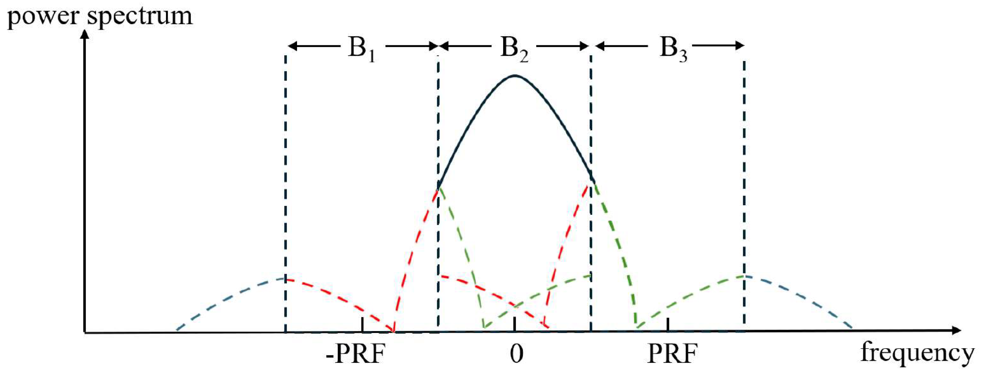
Figure 2.
The structure of echo simulation operator.
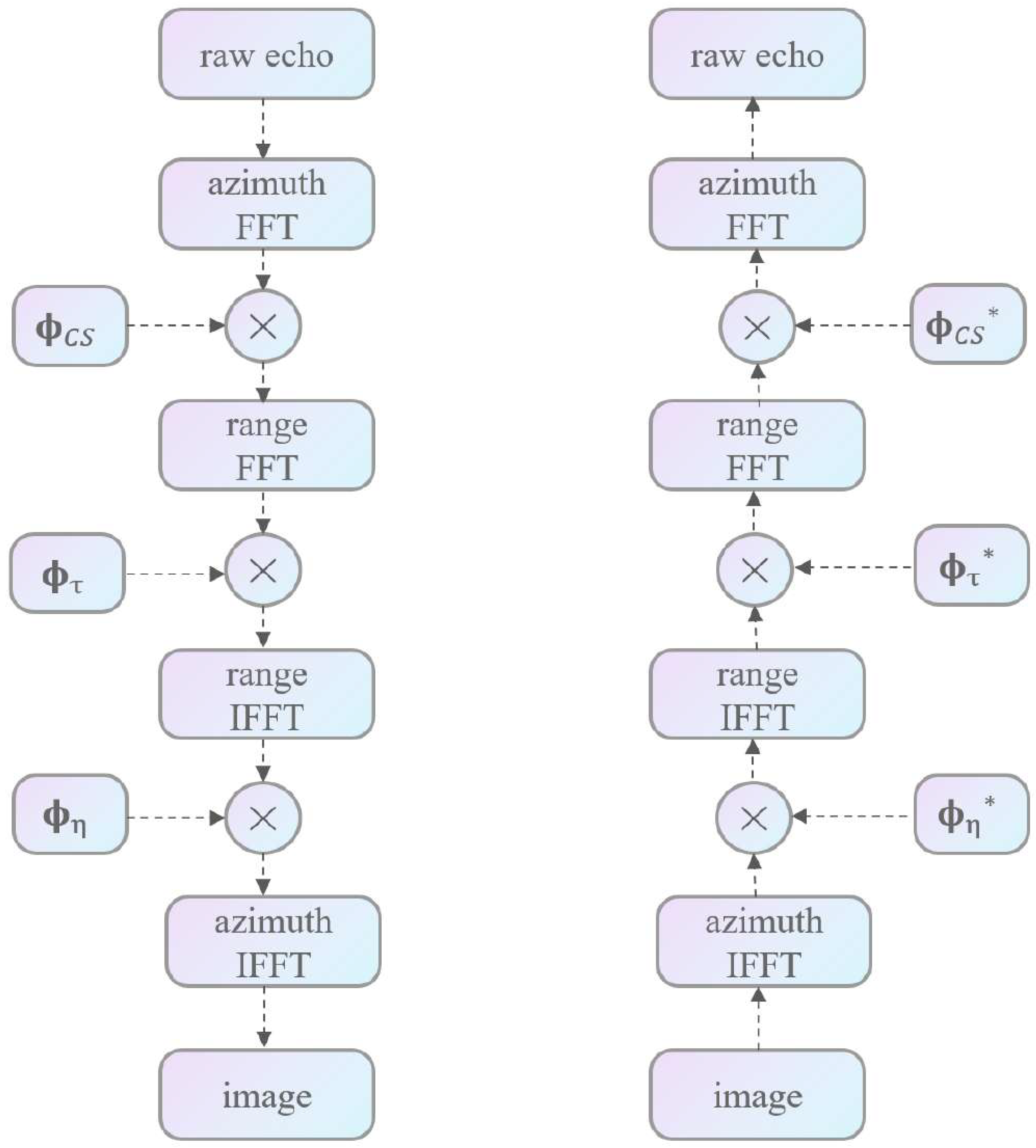
Figure 3.
The iterative process of ISTA-Net.
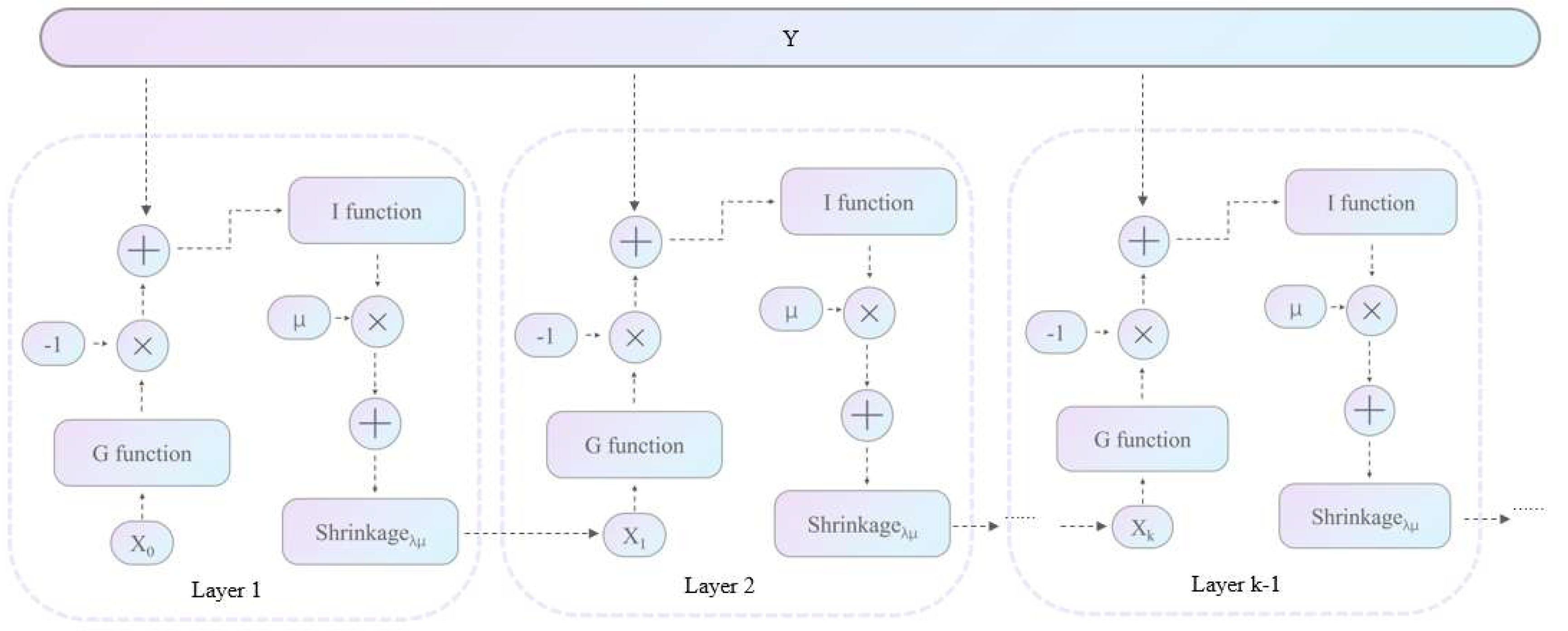
Figure 4.
The iterative process of the algorithm proposed.
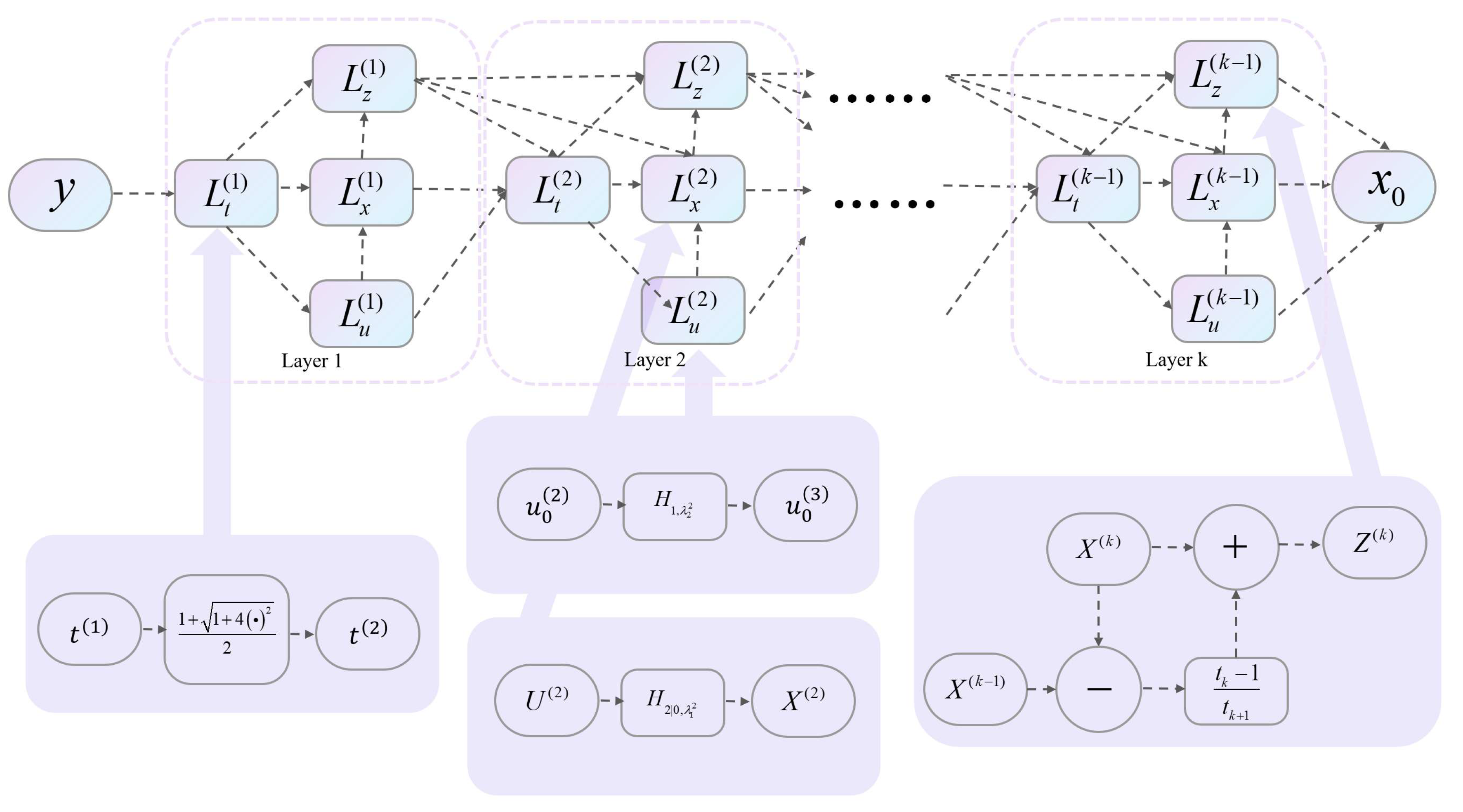
Figure 5.
The structure of SAAS-Net.
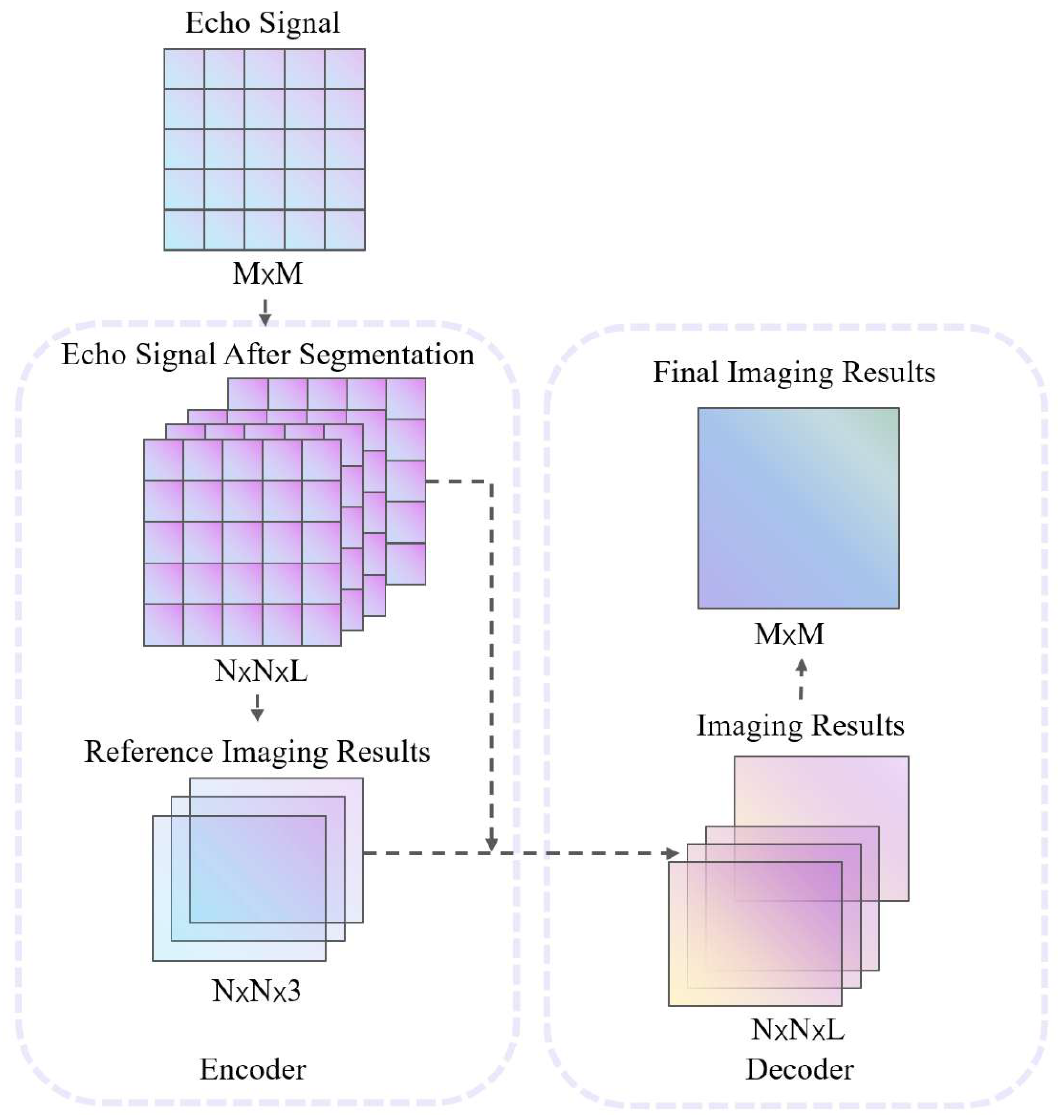
Figure 6.
Point target imaging result(a) The sparse imaging algorithm based on chirp-scaling. (b) The unfolded network based on the chirp-scaling imaging algorithm. (c) The traditional azimuth ambiguity suppression algorithm based on group sparsity. (d) Proposed method.
Figure 6.
Point target imaging result(a) The sparse imaging algorithm based on chirp-scaling. (b) The unfolded network based on the chirp-scaling imaging algorithm. (c) The traditional azimuth ambiguity suppression algorithm based on group sparsity. (d) Proposed method.
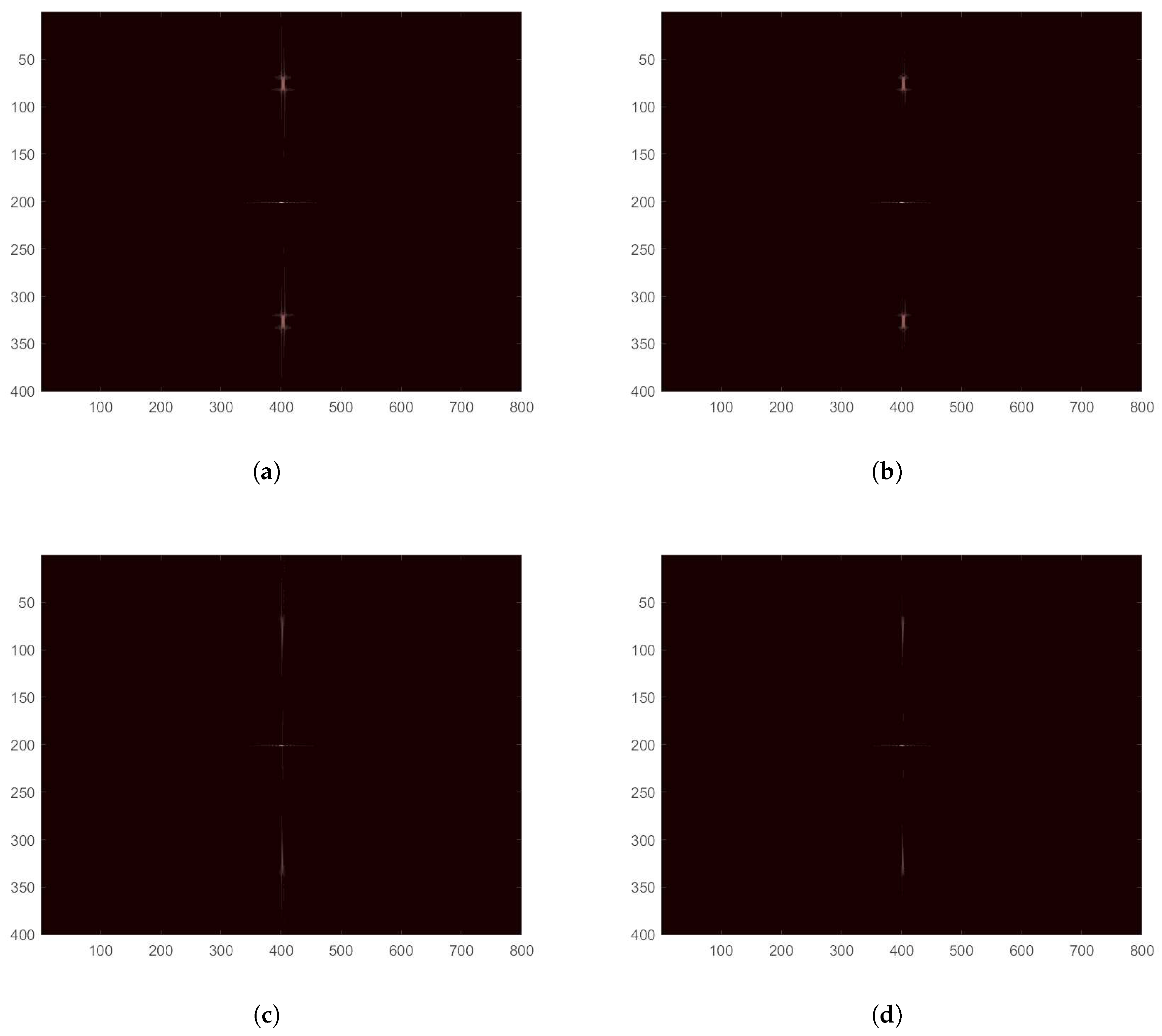
Figure 7.
Azimuth frequency spectrum: (a) The sparse imaging algorithm based on chirp-scaling. (b) The unfolded network based on the chirp-scaling imaging algorithm. (c) The traditional azimuth ambiguity suppression algorithm based on group sparsity. (d) Proposed method.
Figure 7.
Azimuth frequency spectrum: (a) The sparse imaging algorithm based on chirp-scaling. (b) The unfolded network based on the chirp-scaling imaging algorithm. (c) The traditional azimuth ambiguity suppression algorithm based on group sparsity. (d) Proposed method.
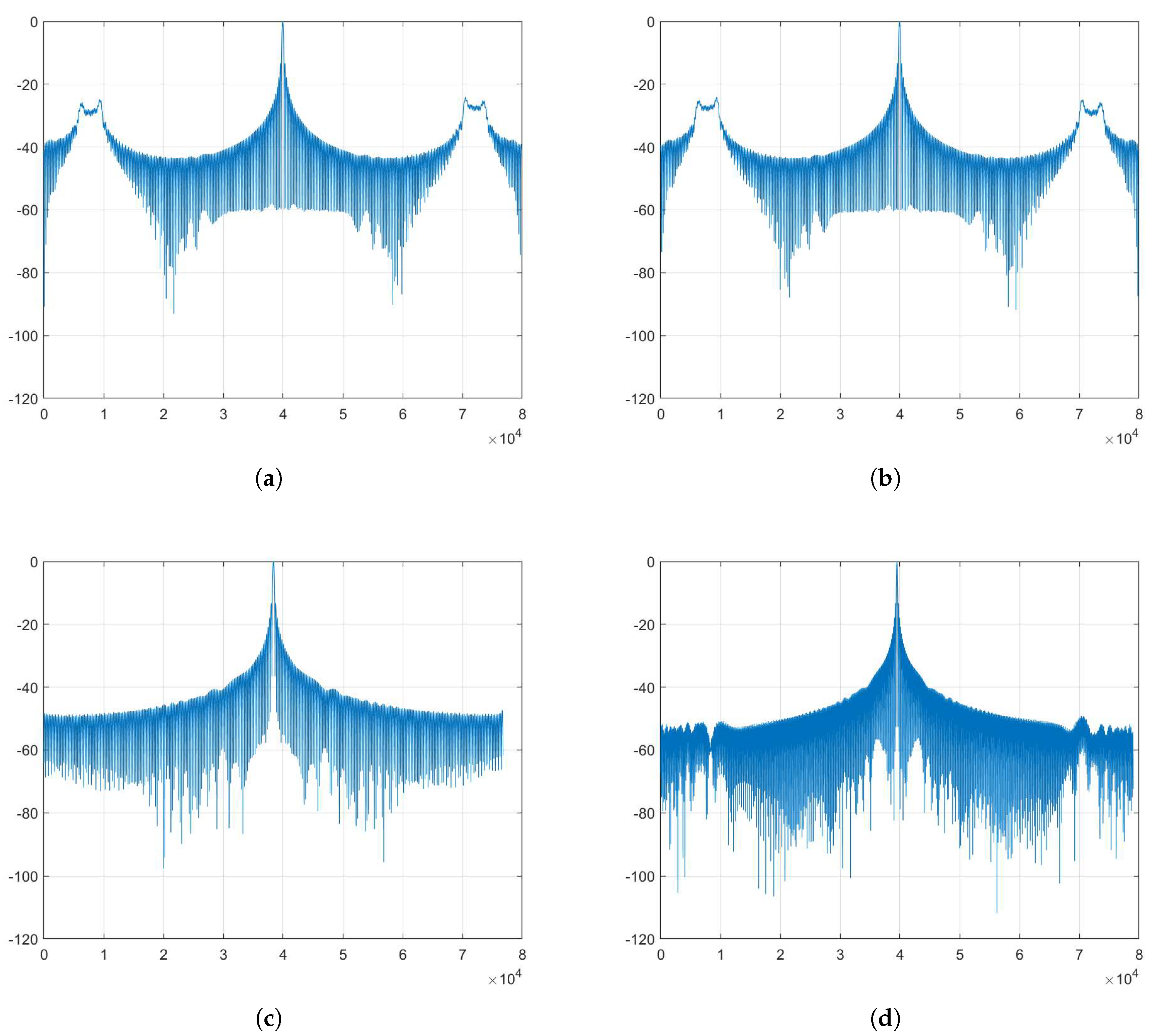
Figure 8.
Realdata imaging result: (a) The sparse imaging algorithm based on chirp-scaling. (b) The unfolded network based on the chirp-scaling imaging algorithm. (c) The traditional azimuth ambiguity suppression algorithm based on group sparsity. (d) Proposed method.
Figure 8.
Realdata imaging result: (a) The sparse imaging algorithm based on chirp-scaling. (b) The unfolded network based on the chirp-scaling imaging algorithm. (c) The traditional azimuth ambiguity suppression algorithm based on group sparsity. (d) Proposed method.
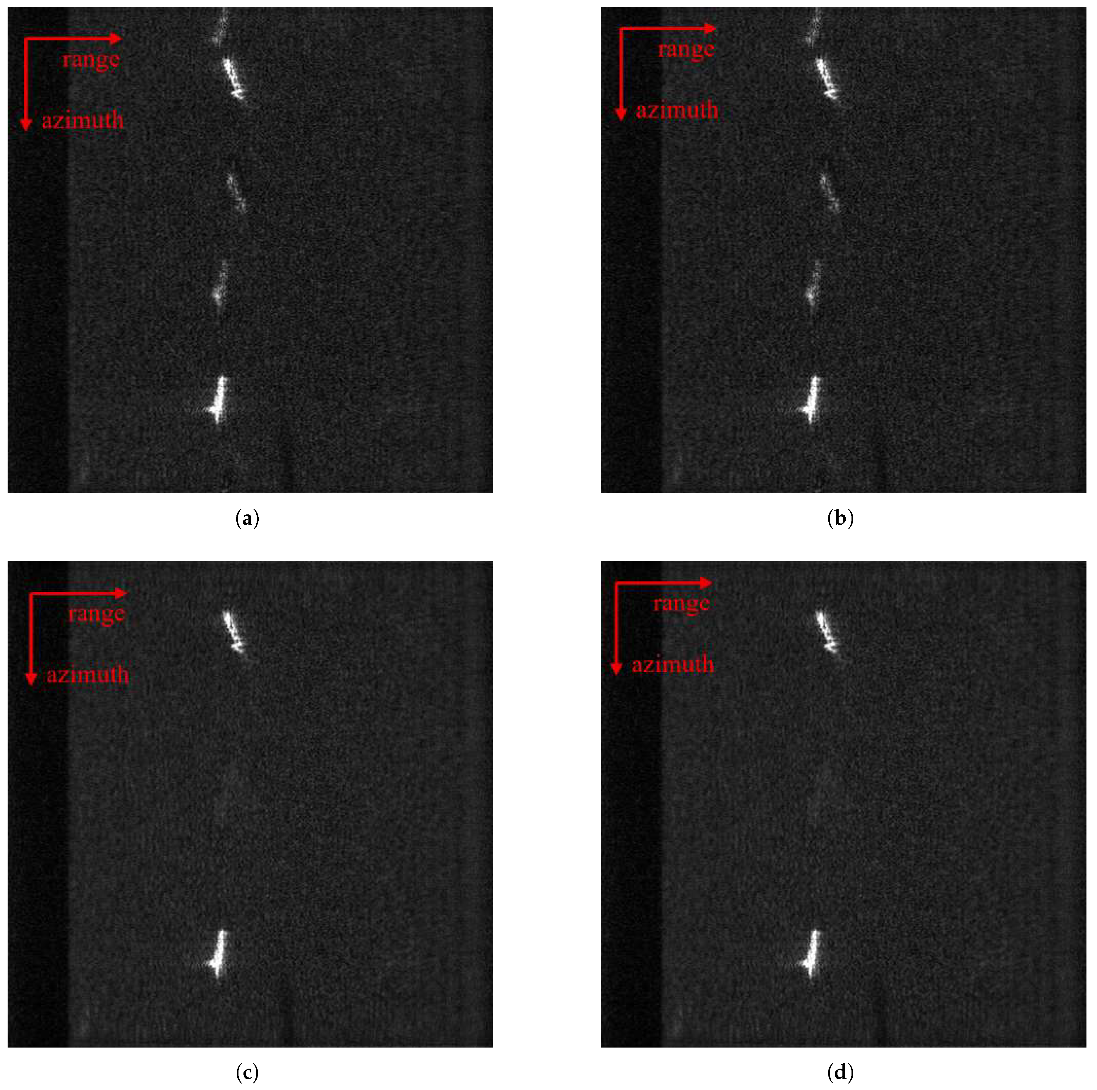
Figure 10.
The imaging result after azimuth downsampling: (a) is the result of ISTA-Net with 80% azimuth downsampling. (b) is the result of AAS-Net with 80% azimuth downsampling.(c) is the result of ISTA-Net with 60% azimuth downsampling.(d) is the result of AAS-Net with 60% azimuth downsampling.(e) is the result of ISTA-Net with 30% azimuth downsampling.(f) is the result of AAS-Net with 30% azimuth downsampling.
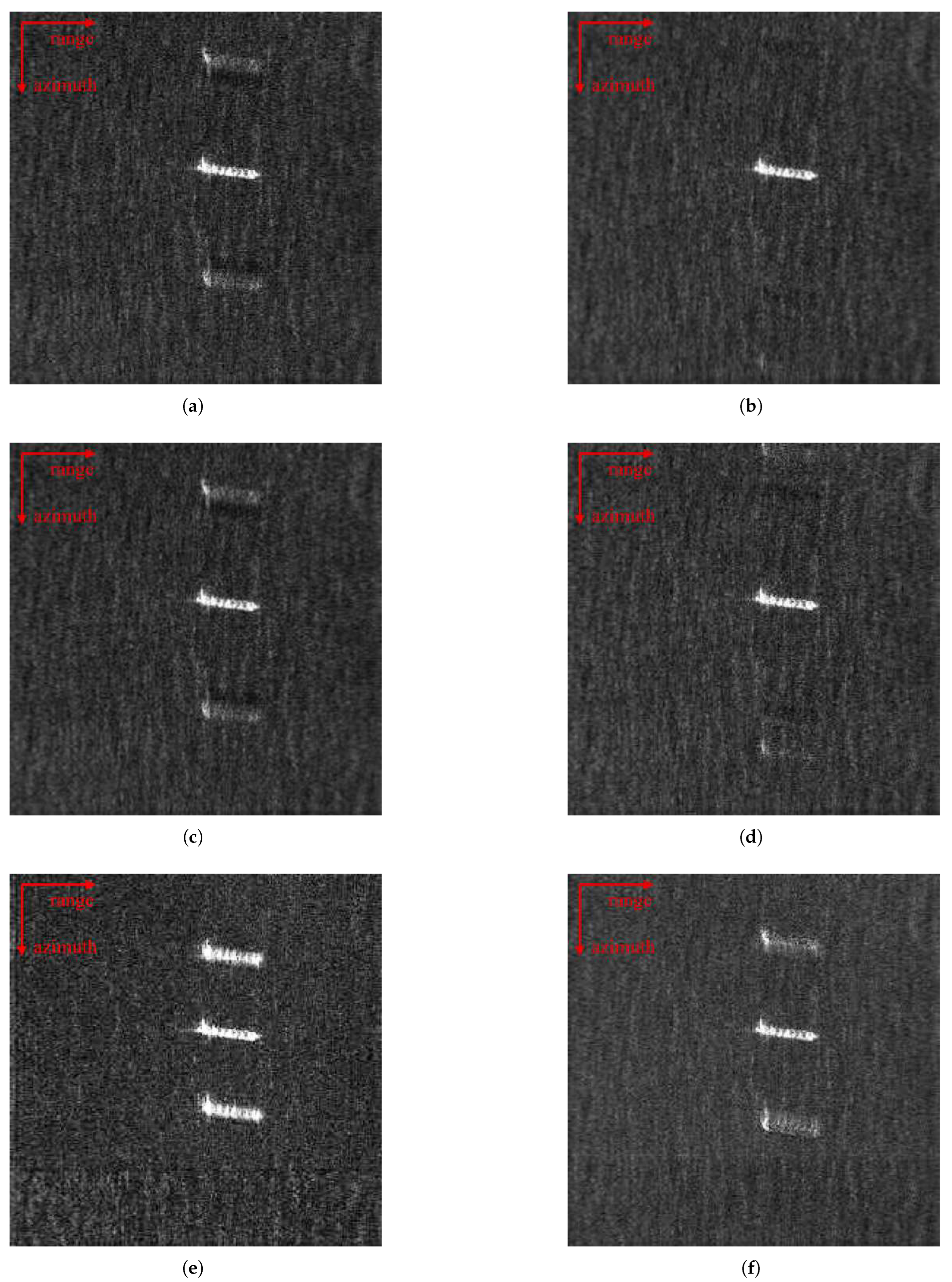
Figure 11.
Imaging results with different iteration layers: (a) Layer 1. (b) Layer 3. (c) Layer 5. (d) Layer 7.
Figure 11.
Imaging results with different iteration layers: (a) Layer 1. (b) Layer 3. (c) Layer 5. (d) Layer 7.
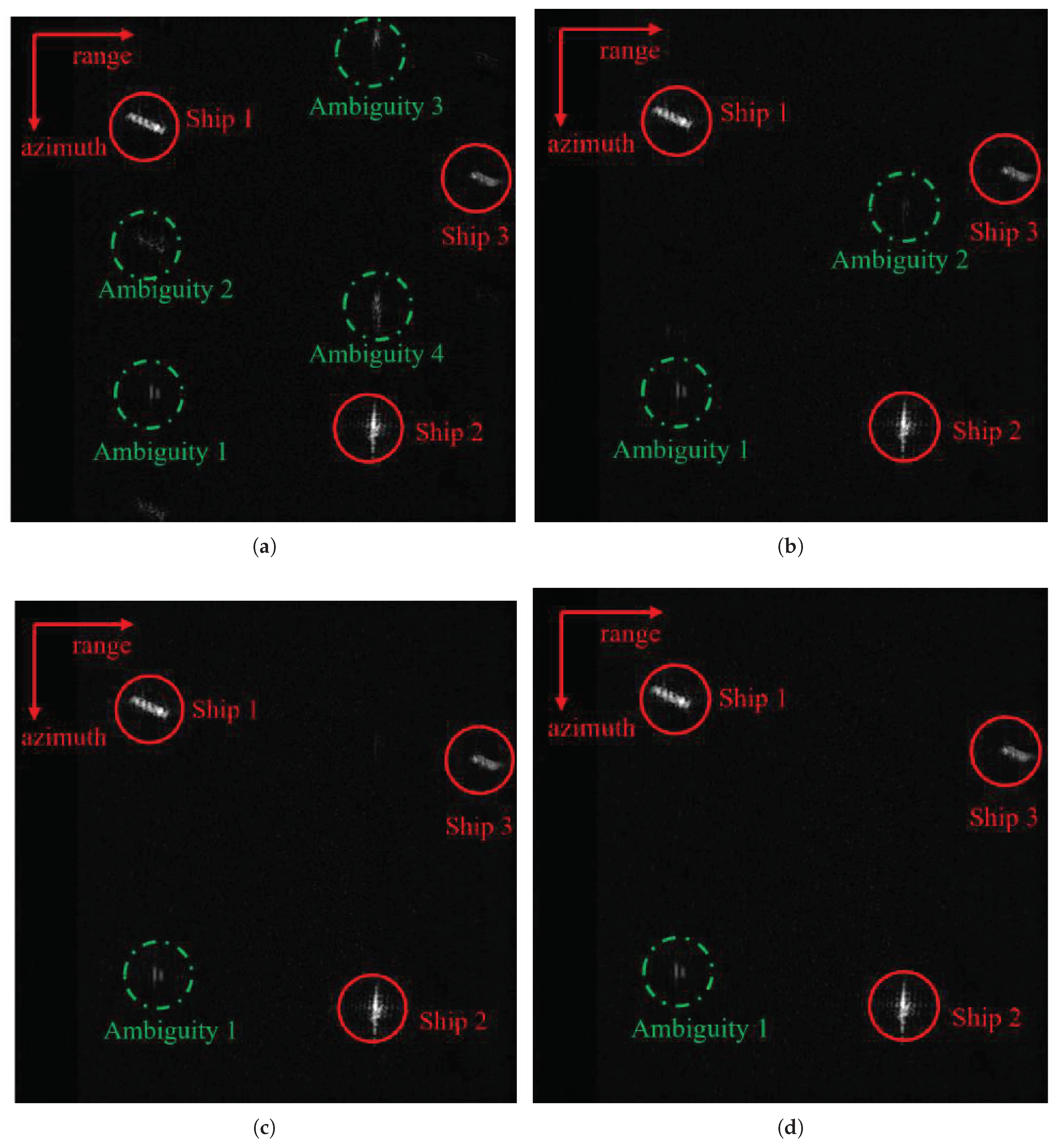

Table 1.
Parameters value of the simulation experiment.
| simulation parameters | value |
|---|---|
| Carrier Frequency/Hz | 1.2e8 |
| Equivalent Bandwidth/m | 1e8 |
| Radar Platform Movement Speed/m/s | 154 |
| SNR/dB | 30 |
| PRF/Hz | 7.2e7 |
| Range/m | 5000 |
Table 2.
Numerical results of the point target simulation experiment.
| Method | PSNR(dB) | ISLR(dB) | AASR(dB) |
|---|---|---|---|
| CS-IST | -13.356 | -10.581 | -14.216 |
| CS-IST-AAS | -19.775 | -16.449 | -17.423 |
| ISTA-Net | -13.542 | -11.325 | -14.198 |
| AAS-Net | -20.194 | -17.232 | -18.017 |
Table 3.
AASR under different undersampling patterns .
| Sample rate | SNR(dB) | CS-IST | CS-IST-AAS | ISTA-Net | AAS-Net |
|---|---|---|---|---|---|
| 20 | -18.15 | -18.34 | -18.07 | -18.46* | |
| 90% | 10 | -18.68 | -19.32* | -18.99 | -19.08 |
| 5 | -19.24 | -19.95 | -18.97 | -20.23* | |
| 20 | -14.22 | -17.42 | -14.20 | -18.02* | |
| 70% | 10 | -15.75 | -17.94 | -14.68 | -18.27* |
| 5 | -16.08 | -18.27 | -16.33 | -18.35* | |
| 20 | -9.15 | -12.36 | -10.32 | -12.73* | |
| 30% | 10 | -10.21 | -12.84 | -10.83 | -13.02* |
| 5 | -10.32 | -13.21 | -11.07 | -13.29* |
Table 4.
Comparisons of AASR for area target.
| Method | AASR(dB) | Time(s)) |
|---|---|---|
| CS-IST | -9.56 | 71.71 |
| CS-IST-AAS | -14.63 | 128.28 |
| ISTA-Net | -11.34 | 0.13 |
| Proposed method | -15.01 | 0.14 |
Disclaimer/Publisher’s Note: The statements, opinions and data contained in all publications are solely those of the individual author(s) and contributor(s) and not of MDPI and/or the editor(s). MDPI and/or the editor(s) disclaim responsibility for any injury to people or property resulting from any ideas, methods, instructions or products referred to in the content. |
© 2025 by the authors. Licensee MDPI, Basel, Switzerland. This article is an open access article distributed under the terms and conditions of the Creative Commons Attribution (CC BY) license (http://creativecommons.org/licenses/by/4.0/).
Copyright: This open access article is published under a Creative Commons CC BY 4.0 license, which permit the free download, distribution, and reuse, provided that the author and preprint are cited in any reuse.


