Submitted:
22 January 2025
Posted:
23 January 2025
You are already at the latest version
Abstract
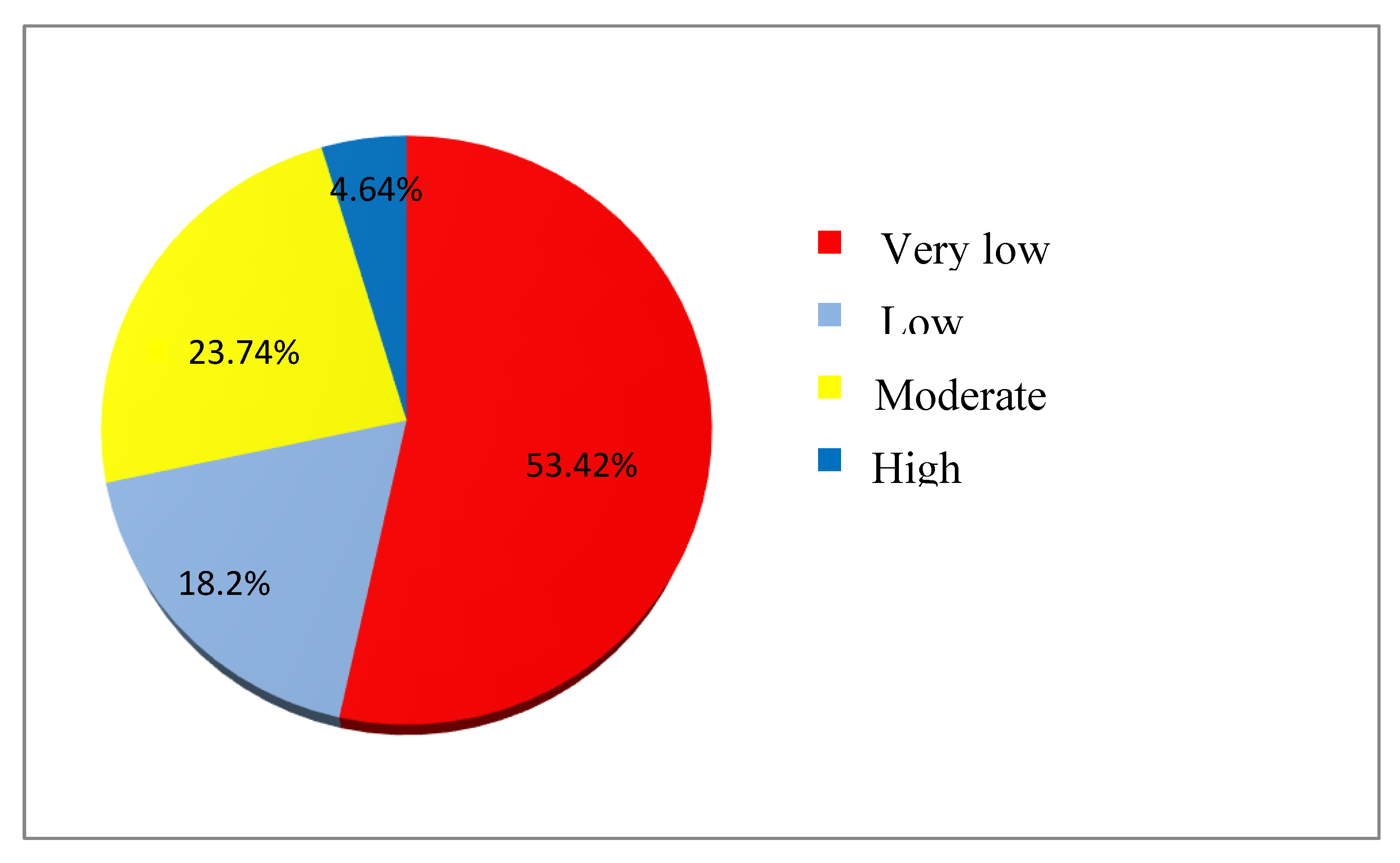
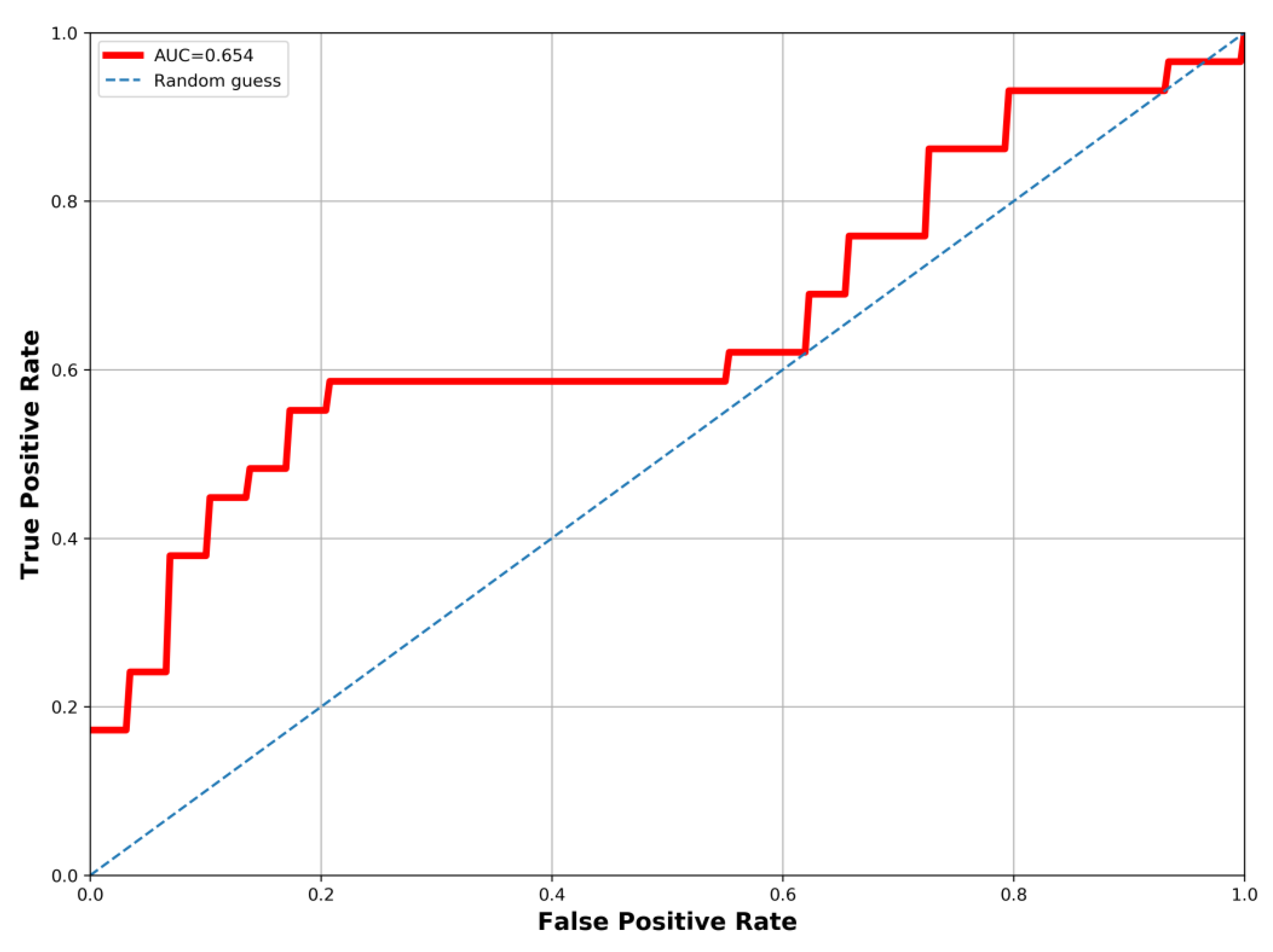
Today, groundwater potential zones (GWPZ) modeling based on scientific principles and modern techniques is a major challenge for scientists around the world. This challenge is even greater in arid and semi-arid areas. Unmanned aerial vehicle (UAV), geographic information system (GIS) and multi-criteria decision making (MCDM) are modern techniques used in various fields of application, particularly in groundwater exploration. This study attempts to use a workflow for modeling the GWPZ using UAV technology, GIS and the MCDM in semi-arid zones. Aerial survey produced a high-resolution DEM of 4 cm. Six influencing factors, including elevation model, drainage density, lineament density, slope, flood zone and topographic wetness index were considered for the delineation of the GWPZ. Four classes of groundwater potential were identified, high (4.64%), moderate (23.74%), low (18.2%) and very low (53.42%). Three validation methods were used, namely, borehole yield data, receiver operating characteristic-area under the curve (ROC-AUC), and principal component analysis (PCA) and gave accuracies of 82.14%, 65.4% and 72.49%, respectively. These validation indicate satisfactory accuracy and justifies the effectiveness of the approach. The mapping of GWPZ in semi-arid zones are very essential for the availability, planning of water resources management and help in sustainable development.
Keywords:
1. Introduction
2. Materials and Methods
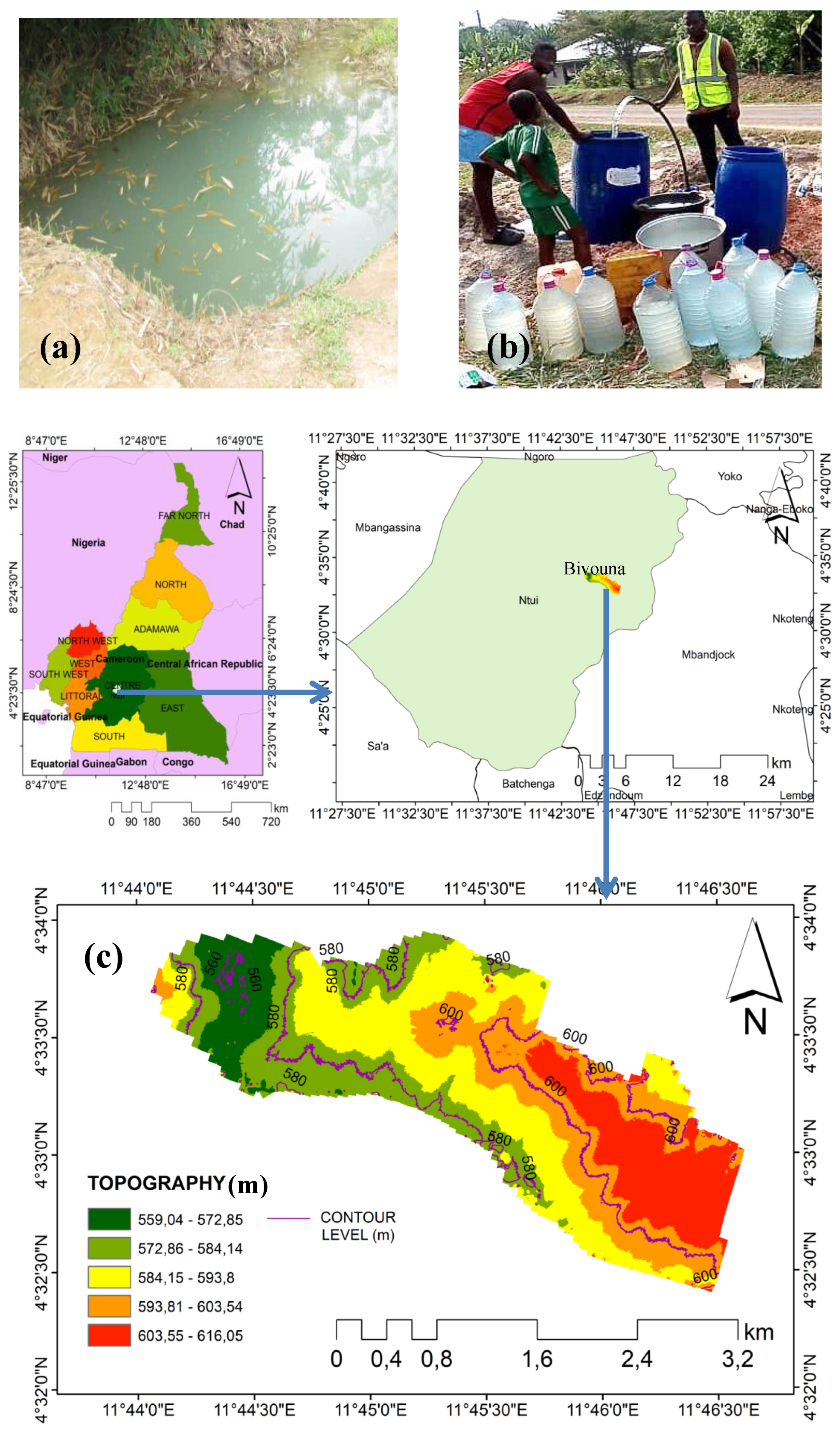
2.1. Study Area
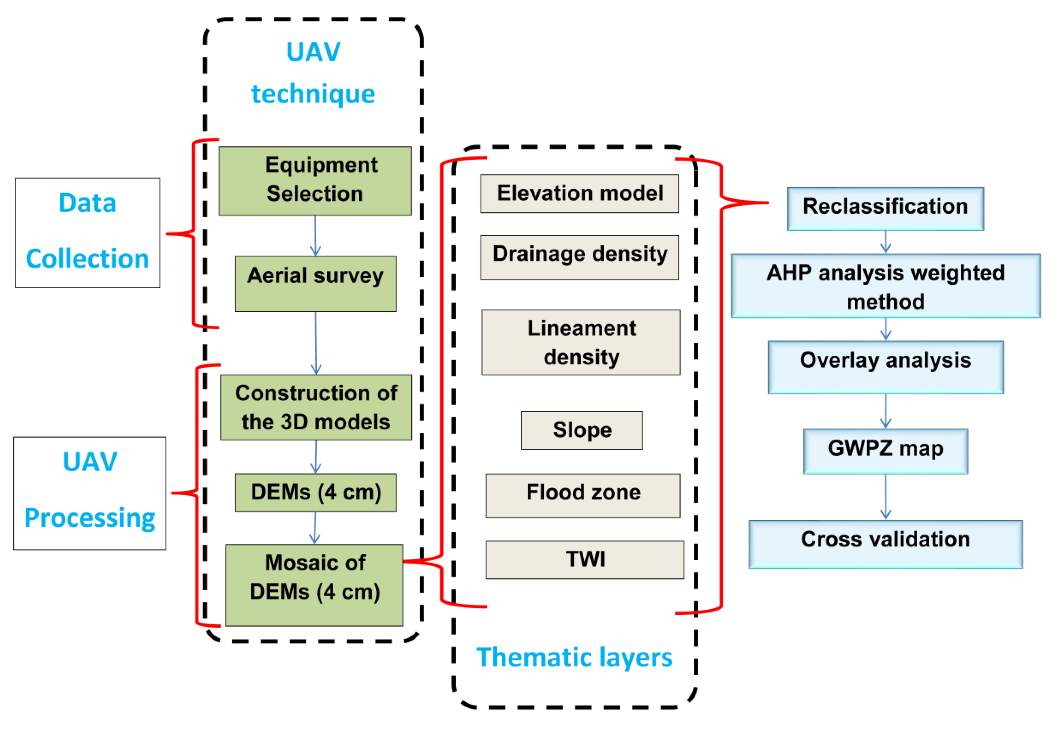
2.2. Workflow
2.3. UAV Technique
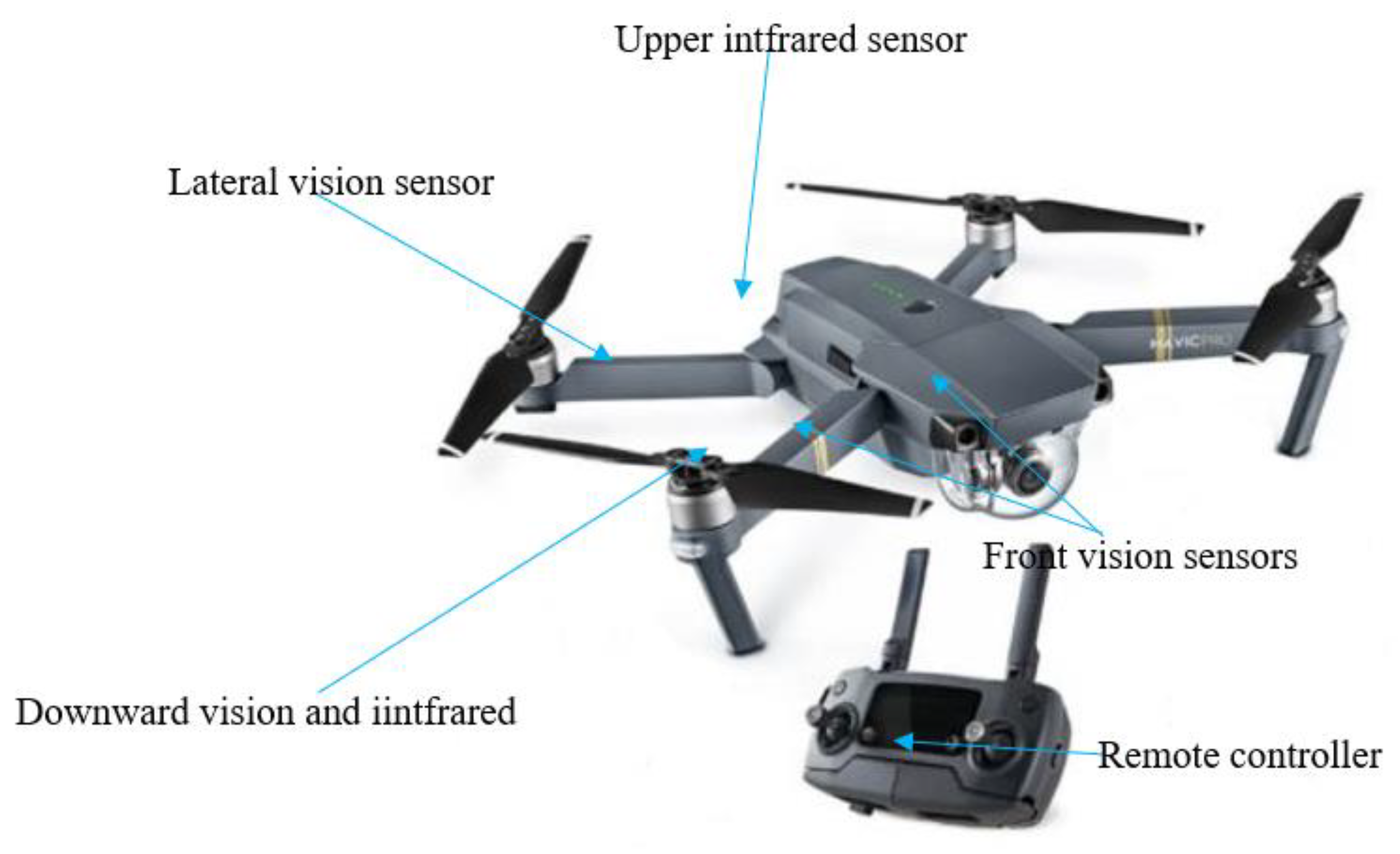
2.3.1. Equipment
2.3.2. Data Collection
2.3.3. UAV Processing
2.4. Generation of Thematic Layers by GIS
2.5. AHP Model
2.5.1. Assigning Ranks and Weights Using AHP
Saaty’s Scale
Standardization of Thematic Layers
2.5.2. Weighting of Determining Factors
Pairwise Comparison
Normalized Weight
2.5.3. Assessing of Matrix Consistency
2.6. Deriving GWPZ
3. Results and Discussion
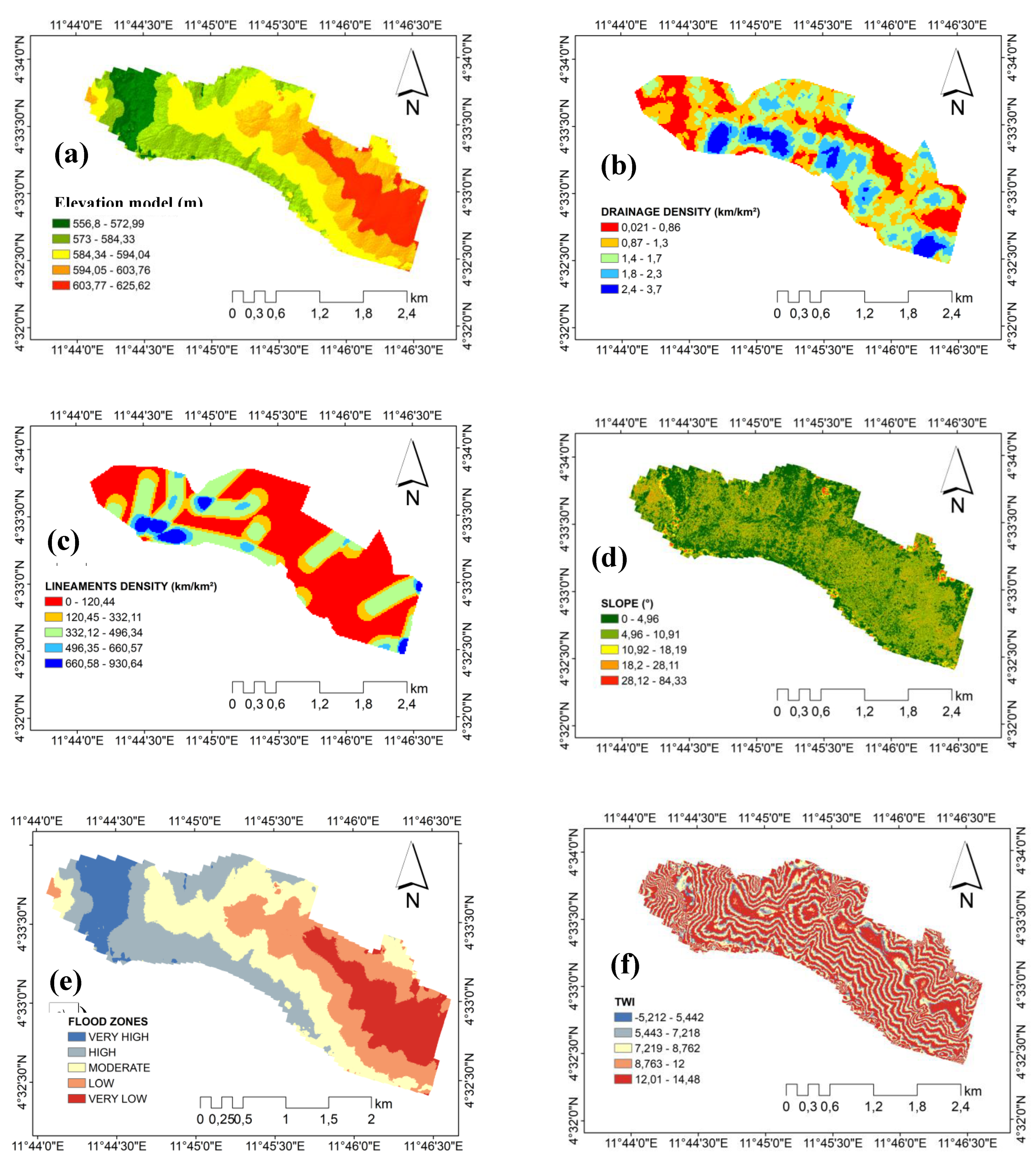
3.1. Thematic Maps
3.1.1. Elevation Model
3.1.2. Drainage Density
3.1.3. Lineament Density
3.1.4. Slope
3.1.5. Flood Zone
3.1.6. Topographic Wetness Index
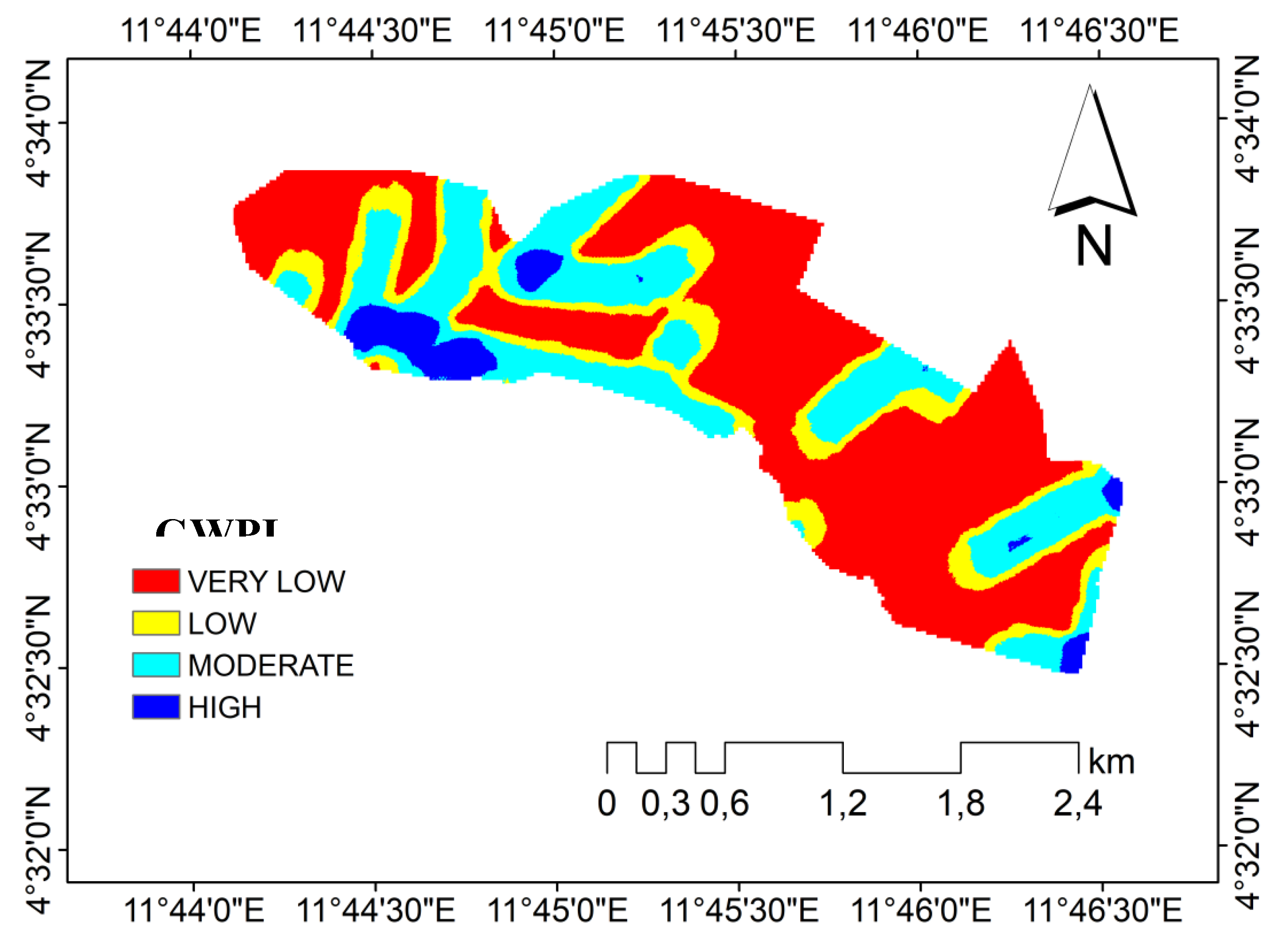
3.1.7. Groundwater Potential Index
3.2. Model Validation
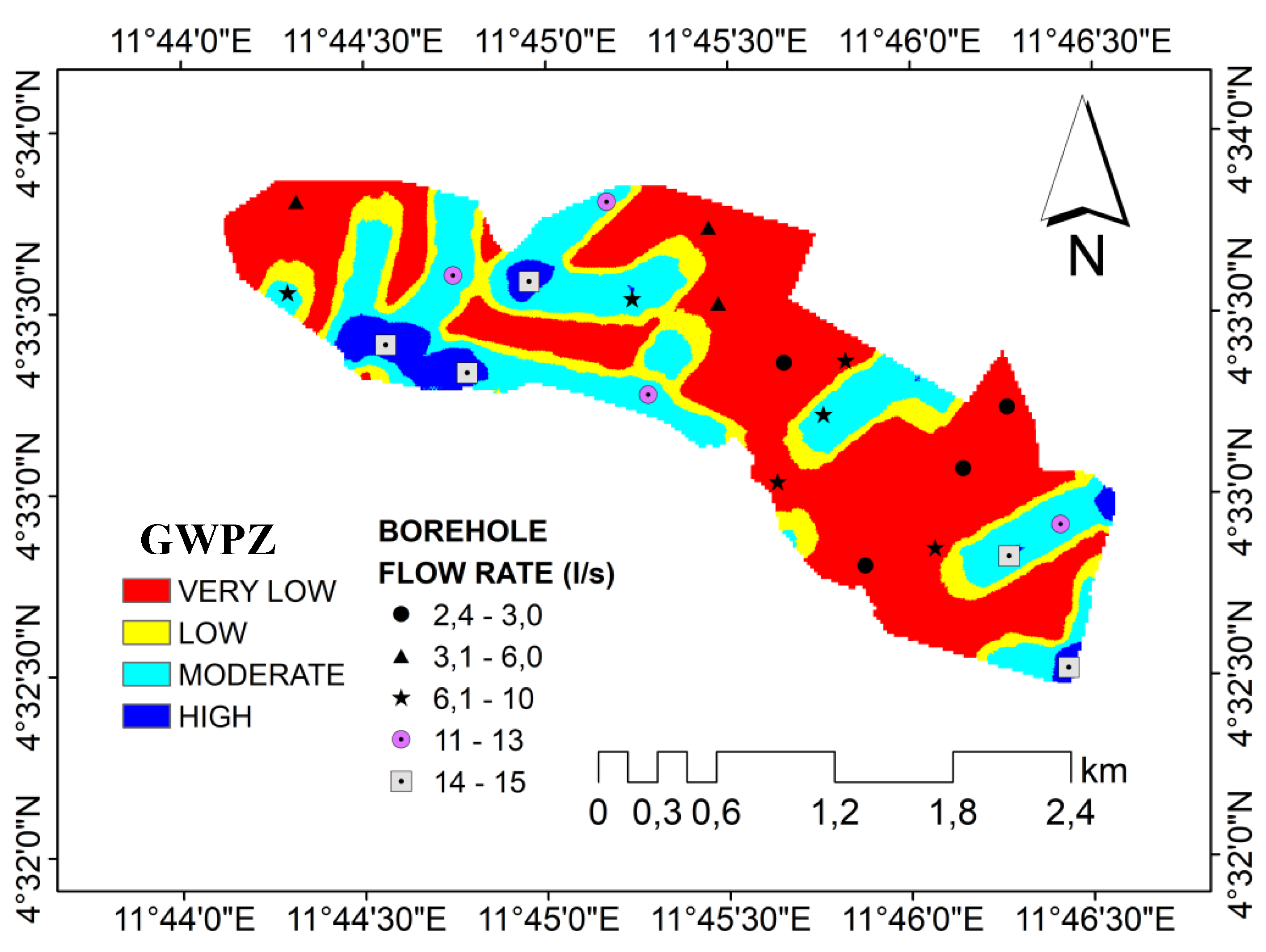
3.2.1. Validation with Borehole Yield Data
3.3.2. ROC-AUC
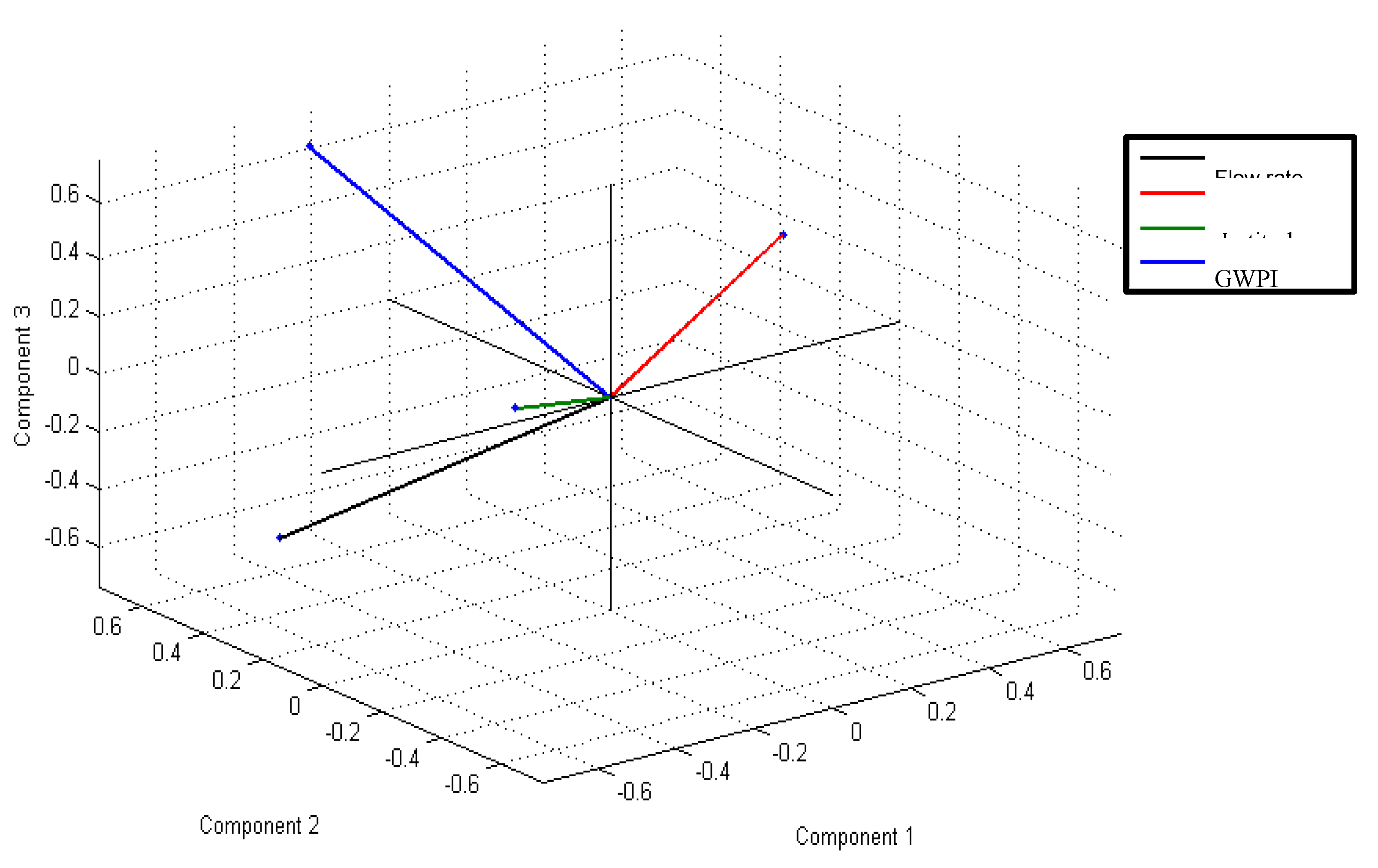
3.3.3. PCA Validation
4. Conclusions
Author Contributions
Funding
Data Availability Statement
Conflicts of interest
References
- Wheater, H.S; Gober, P. Water security and the science agenda. Water Resources Research 2015, 51(7), 5406-5424. [CrossRef]
- Thapa, R; Gupta, S; Guin, S; kaur, H. Assessment of groundwater potential zones unsing multi-inluencing factor (MIF) and GIS: a case study from Birbhum district, west Bengal. Applied water science 2017, 7(7), 4117–4131.
- Das, N; Sutapa, M. Application of multi-criteria making technique for the assessment of groundwater potential zones: a study on Birbhum district, West Bengal, India. Environment Development and Sustainability 2018, 22 (2), 931-955.
- Elshall, A S; Arik, A D; El-Kadi, A. I; Pierce, S; Ye, M; Burnett, K. M; Wada, C. A; Bremer, L.L; Chun, G. Groundwater sustainability: A review of the interactions between science and policy. Environmental Research Letters 2020, 15(9), 093004. [CrossRef]
- Abdo, H.G; Vishwakarma, D.K; Alsafadi, K; Bindajam, A.A; Malick, J; Malick, S. K; Kuma, K.C.A ; Kuriqi, J.A.A; Artan Hysa, A. GIS-based multi-criteria decision making for delineation of potential groundwater recharge zones for sunstainable resource management in the Eastern Mediteranean: a case study. Applied water science 2024, 14: 160, 1-19.
- El-Sayed, H.M; Elgendy, A.R. Geospatial and geophysical insights for groundwater potential zones mapping and aquifer evaluation at Wadi Abu Marzouk in ElNagila, Egypt. The Egyptian Journal of Aquatic Research 2024, 50(1), 23-35. [CrossRef]
- World Health Organization (WHO). Report on surveillance of antibiotic consumption: 2016–2018 early implementation. World Health Organization 2018.
- UN (United Nation). Report on sustainable development objectives. United Nation 2019.
- World Health Organization (WHO). A global overview of national regulations and standards for drinking-water quality. 2nd ed. Geneva: World Health Organization 2021. ISBN 978-92-4-002364-2.
- Anusha,B.N; Babu, K.R; Kumar,B.P; Kumar, P.R; M. Rajasekhar, M. Geospatial approaches for monitoring and mapping of water resources in semi-arid regions of southern India. Environmental challenges 2022, 8, 100569. [CrossRef]
- Das, S. C; Akhtar, F; Alrasheedi, A. F; Akbar, A.C. Application of water cycle algorithm with demand follows green level and nonlinear power pattern of the product for an inventory system. Scientific Reports 2024, 14(1), 20995.
- Franke, J. Drying groundwater. Nature Climate Change 2024, 14(8), 896.
- Rohde, M. M; Albano , C. M; Huggins, X; Kirk R; Klausmeyer, K.R; Charles Morton, C; Sharman, A; Zaveri, E; Laurel Saito, L; Freed, Z; Howard, J.K; Job, N; Richter, H; Toderich, K; Rodella, A.S; Gleeson, T; Huntington, J; Chandanpurkar, H.A; Purdy, A.J; Famiglietti, J.S; Singer, M.B; Dar A. R; Caylor, K; John C. S. Groundwater-dependent ecosystem map exposes global dryland protection needs. Nature 632 2024, 101–107. [CrossRef]
- Turner; S. W. D; Rice, J.S; Nelson K.D; Vernon, C.R; McManamay, R ; Dickson, K;Marston, L. Comparison of potential drinking water source contamination across one hundred U.S. cities. Nature communication 2021, 12:7254 . [CrossRef]
- Hashimoto, R; Kazama, S; Hashimoto, T; Oguma, K; Satoshi Takizawa, S. Planning methods for conjunctive use of urban water resources based on quantitative water demand estimation models and groundwater regulation index in Yangon City, Myanmar. Journa of cleaner production 2022, 367(133121): 0959-6526. [CrossRef]
- Minuyelet, Z.M; Kasie, L.A; Bogale, S. Groundwater potential zones delineation using GIS and AHP techniques in upper parts of Chemoga watershed, Ethiopia. Applied Water Science 2024, 14, 85. [CrossRef]
- Mir M. R; McDermid. G. J; Strack , M; Lovitt J. A New Method to Map Groundwater Table in Peatlands Using Unmanned Aerial Vehicles. Remote Sensing 2017, 9, 1057. [CrossRef]
- Chen , W ; Tsangaratos, P ; Ilia, I ; Duan, Z; Chen, X. Groundwater spring potential mapping using population-based evolutionary algorithms and data mining methods. Science of the Total Environment 2019, 684, 31–49. [CrossRef]
- Smith, C; Satme, J; Martin, J; Downey, A.R.J ; Vitzilaios, N; Imran, J. UAV rapidly-deployable stage sensor with electro-permanent magnet docking mechanism for flood monitoring in undersampled watersheds. HardwareX 2022, 12, 2468-0672. [CrossRef]
- Bhuyan, M.J; Deka, N. Delineation of groundwater potential zones at micro-spatial units of Nagaon district in Assam, India, using GIS-based MCDA and AHP techniques. Environmental Science and Pollution Research 2022, 3, 54107-54128.
- Orojah, J.O; Eshimiakhe, D; Oniku A.S; Kolawole, M.L. Application of remote sensing and electrical resistivity technique for delineating groundwater potential in North Western Nigeria. Scientific reports 2024, 14, 22299.
- EL-Bana, E.M.M; Alogayell, H.M; Sheta, H.M; Mohamed Abdelfattah, M. An integrated remote sensing and GIS-based technique for mapping groundwater recharge zone: A case study of SW Riyadh, Central Saudi Arabia. Hydrology 2024, 11, 38.
- Acharya, B.S; Bhandari, M; Bandini, F; Pizarro, A; Perks, M; Joshi, R.D; Wang, S; Dogwiler, T; Rai, R.L; Kharel, G; Sharma, S. Unmanned aerial vehicles in hydrology and water management applications, challenges, and perspectives. Water resources research 2021, 57 (11), 1944-7973.
- Vellemu, E.C; Katonda, I; Abiou, V; Yapuwa, H; Msuku, G; Nkhoma, S; Makwakwa, C; Safuya, K; Maluwa, A. Using the Mavic 2 Pro drone for basic water assessment. Scientific African 2021, 14(3), e00979. [CrossRef]
- Vélez, N. M; García, L.S; Barbero, L; Verónica Ruiz, O; Sánchez, B.A. Applications of Unmanned Aerial Systems (UASs) in Hydrology: A Review. Remote Sensing 2021, 13, 1359.
- Lee, E; Park, S; Jang, H; Choi, W; Sohn, H.G. Enhancement of low-cost UAV-based photogrammetric point cloud using MMS point cloud and oblique images for 3D urban reconstruction. Measurement 2024, 226,114158. [CrossRef]
- Liu, Z; Li, J; Shen, J; Wang, X; Chen, P. Leader–follower UAVs formation control based on a deep Q-network collaborative framework. Scientific Reports 2024, 14, 4674. [CrossRef]
- Román, A ; Navarro, G ; Tovar, A.S ; Zarandona, P ; Roque, D.A ; Barbero, L. Shetlands UAV metry: unmanned aerial vehicle-based photogrammetric dataset for Antarctic environmental research. Scientific Data 2024, 11, 202.
- Rui, Y; Wang, C; Barton,N ; Du, S. A photogrammetric approach for quantifying the evolution of rock joint void geometry under varying contact states, International Journal of Mining Science and Technology 2024, 34(4), 461-47. [CrossRef]
- Kouamou, N.S.R; Enyegue, A.N.F.M.; Bikoro, B.M; Tchikangoua, N.A; Tabod, C.T. Modeling groundwater potential zones in the Kribi-Campo region, South Cameroon using geospatial techniques and statistical models. Modelling Earth System and Environment 2022.
- Vellaikannu, A ; Palaniraj, U; Karthikeyan, S; Senapathi, V; Viswanathan, P. M, Sekar, S. Identification of groundwater potential zones using geospatial approach in Sivagangai district, South India. Arabian Journal of Geosciences 2021, 14(1), 8. [CrossRef]
- Shebl, A; Abdelaziz, M. I; Ghazala, H; Awad, S. S. A; Abdellatif, M; Csámer, A. Multi-criteria ground water potentiality mapping utilizing remote sensing and geophysical data: A case study within Sinai Peninsula. The Egyptian Journal of Remote Sensing and Space Sciences 2022, 25(3), 765–778. [CrossRef]
- Ikrri, M; Boutaleb, I; Abiou, M; Zahra, F.E; Abdelrahman, K; Mouna, I; Tamer, A; Hasna, E.A; Sara, E; Farid, F. Delineation of groundwater potential area using an AHP, remote sensing, and GIS Techniques in the Ifni Basin, Western Anti-Atlas, and Morocco. Water 2023, 15(7), 1436.
- Akatsuka,T; Saito, R.; Kajiwara, T; Osada, K.; Nagaso, M; Norihiro, W.N; Tsuchiya, N; Hiroshi, A; Kanetsuki, T. Geothermal geology and comprehensive temperature model based on surface and borehole geology in Sengan, Northeast Japan. Geothermics 2022, 105, 102485. [CrossRef]
- Yeh, H.C; Chen, Y.C; Wei, C. Cross-validation methods in principal component analysis: a comparison. Paddy water environ 2013, 11(1), 71–82.
- Kamijo, T; Chen, Y.C; Wei, C. A verification of alternative assessment using principal component analysis based on case studies of the japan international cooperation agency. Paddy water environ 2014, 45(5), 31–38.
- Kong, G; Jiang, L; Yin, X.; Wang, T; Xu, D.L; Ruiz, O.V; Y, J.B; Hu, Y. Combining principal component analysis and the evidential reasoning approach for healthcare quality assessment. Ann oper res 2018, 271(2), 679–699. [CrossRef]
- Giancarlo, D; Chiara, T. Cross-validation methods in principal component analysis: a comparison. Statistical methods and applications 2002, 11(1), 71–82.
- Ngnotué, T; Nzenti, J.P; Sing, A., Barbey, P; Tchoua, F.M. The Ntui-Betamba high-grade gneiss: a northward extension of the pan-afriacn Yaoundé gneiss in cameroon. Journal of african earth science 2000, 31(2), 1464–343X.
- Beni, T; Borselli, D; Bonechi,L.,Lombardi, L; Gonzi, S; Melelli, M; Turchetti , M.A; Fanò, L; Alessandro,R.; Gigli, G; Casagli, N. Laser scanner and UAV digital photogrammetry as support tools for cosmic-ray muon radiography applications: An archaeological case study from Italy. Scientific Reports 2023, 13, 19983. [CrossRef]
- Yeh, H.F; Cheng, Y.S; Lin, H.I; Lee, C.H. Mapping groundwater recharge potential zone using a GIS approach in Hualian River. Taiwan. Sustainable Environment Research 2016, 26(1), 33–43. [CrossRef]
- Garcia, L.S; Velez, N.M; Martinez, L.J; Bellon, S.A; Pacheko, O.M.J; Ruiz, O.V; Munoz, J.J.P; Barbero, L. Using UAV photogrammetry and automated sensors to assess aquifer recharge from a coastal wetland. Remote sensing 2022, 14(24), 6185.
- Arulbalaji, P; Padmalal, D; Sreelash, K. GIS and AHP Techniques Based Delineation of Groundwater Potential Zones: a case study from Southern Western Ghats, India. Scientific reports 2019, 9, 2082. [CrossRef]
- Abdullahi, A; Muralitharan, J; Getahun, E; Gunalan, J; Abebe, A.. Assessment of potential groundwater Zones in the drought-prone Harawa catchment, Somali region, eastern Ethiopia using geospatial and AHP techniques. The Egyptian Journal of Remote Sensing and Space Sciences 2023, 26, 628–641. [CrossRef]
- El Mekki, A.O; Laftouhi, N.E. Combination of a geographical information system and remote sensing data to map groundwater recharge potential in arid to semi-arid areas: the Haouz Plain, Morocco. Earth Science Informatics 2016, 9(4), 465–479.
- Nshagali, B.G; Meli’i, J. L; Nyouma, R. N; Marcel, J; Oyoa, V; Perilli, N; Nouck, P. N. Groundwater Potential index map and characterization of unconfined aquifers, in crystalline basement region of Cameroon, using Multicriteria Decision Making. Arabian Journal of Geosciences 2022, 15, 1594. [CrossRef]
- Saaty, T. L. How to make a decision: The analytic hierarchy process. European Journal of Operational Research 1990, 48(1), 9–26.
- Patel, A.K; Sharma, M; Sing, A; Dubey, S; Chandola, V.K; Mishra, S. Groundwater potential zones using multi-criteria decision making for Mirzapur, District, U.P, India. International journal of environment and climate change 2024, 14(4), 27–45.
- Saaty, T.L. How to make a decision: The analytic hierarchy process. European Journal of Operational Research 1980, 48:9–26.
- Saaty, T.L. Fundamentals of the analytic network process—multiple networks with benefits, costs, opportunities and risks. J Syst Sci Syst Eng 2004, 13(3):348–379.
- Pouth, N. A. M, Meli’I, J. L, Gweth, M. M., Gounou, P. B. P., Njock, M. C, Teikeu, A. W., Mbouombouo, N.,I., Poufone, Y. K., Wouako, W. R. K. & Njandjock, N. P. An approach to assess hazards in the vicinity of mountain and volcanic areas. Landslides 2024.
- Gweth, M. M. A; Nkoungou, H. E; Meli’i, J. L; Gouet, D. H; Njandjock, N. P. Fractures models comparison using GIS data around crater lakes in Cameroon volcanic line environment. The Egyptian Journal of Remote Sensing and Space Sciences 2021a, 24(2), 419-429. [CrossRef]
- Gweth, M.M.A; Jorelle Larissa Meli'i, J.L; Oyoa, V; Diab, D.A.; Gouet, D.H; Marcel, J; Njandjock, N.P. Fracture network mapping using remote sensing in three crater lakes environments of the Cameroon volcanic line (central Africa). Arabian Journal of Geosciences 2021b, 14(6), 422.
- Poufone, K.P; Meli’i, J.L; Aretouyap, Z; Gweth, M.M.A; Nguemhe, S.C.F; Nshagali, G.B; Oyoa, V; Perilli, N; Njandjock, N.P. Possible pathways of seawater intrusion along the MountCameroon coastal area using remote sensing and GIS techniques. Advances in Space Research 2022, 69(2), 2047–2060.
- Andualem, T. G; Demeke, G.G. Groundwater potential assessment using GIS and remote sensing: A case study of Guna tana landscape, upper Blue Nile Basin, Ethiopia. Journal of Hydrology: Regional Studies 2019, 24, 100610. [CrossRef]
- Tolche, A. D. Groundwater potential mapping using geospatial techniques: a case study of Dhungeta-Ramis sub-basin, Ethiopia. Geology, Ecology, and Landscapes 2020, 5(1), 65–80. [CrossRef]
- Githinji, T. W; Dindi, E. W; Kuria, Z. N; Olago, D. O. Application of analytical hierarchy process and integrated fuzzy-analytical hierarchy process for mapping potential groundwater recharge zone using GIS in the arid areas of Ewaso Ng’iro–Lagh Dera Basin, Kenya. HydroResearch 2022, 5, 22-34. [CrossRef]
- Sulaiman, W. H; Mustafa, Y.T. Geospatial multi-criteria evaluation using AHP- GIS to delineate groundwater potential zones in Zakho Basin, Kurdistan Region, Irak. Earth 2023, 4(3), 655-675.
- Saha, S. Groundwater potential mapping using analytical hierarchical process: a study on Md. Bazar Block of Birbhum District. West Bengal. Spatial Information Research 2017, 25,615–626. [CrossRef]
- Mallick J; Khan R.A; Ahmed M; Alqadhi, S.D; Alsubih, M; Falqi, I; HASSAN, M.A. Modeling groundwater potential zone in a semi-arid region of Aseer using Fuzzy-AHP and geoinformation techniques. Water 2019, 11(12), 2656. [CrossRef]

| Intensity of Importance | Definition |
|---|---|
| 1 | Equal Importance |
| 2 | Equal to moderate importance |
| 3 | Moderate importance |
| 4 | Moderate to strong importance |
| 5 | Strong importance |
| 6 | Strong to very strong importance |
| 7 | Very strong importance |
| 8 | Very to extremely strong importance |
| 9 | Extreme importance |
| Factors | Classes | potentiality | Criterion weight | Rank | Normalized weight |
| EM |  |
Very good Good Medium Poor Very poor |
0.51 0.24 0.13 0.07 0.05 |
5.00 4.00 2.00 1.00 1.00 |
0.36 |
| DD |  |
Very good Good Medium Poor Very poor |
0.44 0.26 0.17 0.09 0.04 |
5.00 4.00 1.00 1.00 1.00 |
0.25 |
| LD |  |
Very poor Poor Moderate Good Very good |
0.41 0,26 0,19 0,09 0,05 |
5.00 3.00 2.00 1.00 1.00 |
0.1630295 |
| SL | 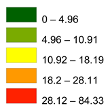 |
Very good Good Moderate Poor Very poor |
0.40 0.22 0.19 0.17 0.02 |
5.00 4.00 3.00 2.00 1.00 |
0.10438802 |
| FZ |  |
Very good Good Moderate Poor Very poor |
0.34 0.23 0.16 0.15 0.12 |
5.00 4.00 3.00 2.00 1.00 |
0.06671751 |
| TWI |  |
Very poor Poor Moderate Good Very good |
0.5 0.3 0.12 0.05 0.03 |
5.00 4.00 3.00 2.00 1.00 |
0.0493883 |
| EM | DD | LD | SL | FZ | TWI | |
|---|---|---|---|---|---|---|
| EM | 1 | 2 | 3 | 4 | 5 | 4 |
| DD | 0.5 | 1 | 2 | 3 | 4 | 5 |
| LD | 0.333 | 0.5 | 1 | 2 | 3 | 4 |
| SL | 0.25 | 0.333 | 0.5 | 1 | 2 | 3 |
| FZ | 0.2 | 0.25 | 0.333 | 0.5 | 1 | 2 |
| TWI | 0.25 | 0.2 | 0.25 | 0.333 | 0.5 | 1 |
| EM | DD | LD | SL | FZ | TWI | Criteria weight | |
|---|---|---|---|---|---|---|---|
| EM | 0.39473684 | 0.46692607 | 0.42352941 | 0.36923077 | 0.32258065 | 0.21052632 |
0.028 |
| DD | 0.19736842 | 0.23346304 | 0.28235294 | 0.27692308 | 0.25806452 | 0.26315789 |
0.014 |
| LD | 0.13157895 | 0.11673152 | 0.14117647 | 0.18461538 | 0.19354839 | 0.21052632 |
0.021 |
| SL | 0.09868421 | 0.07782101 | 0.07058824 | 0.09230769 | 0.12903226 | 0.15789474 |
0.030 |
| FZ | 0.07894737 | 0.05836576 | 0.04705882 | 0.04615385 | 0.06451613 | 0.10526316 |
0.026 |
| TWI | 0.09868421 | 0.04669261 | 0.03529412 | 0.03076923 | 0.03225806 | 0.05263158 |
0.016 |
| n | 2 | 3 | 4 | 5 | 6 | 7 | 8 | 9 | 10 | 11 | 12 | 13 | 14 |
| RI | 0 | 0.52 | 0.9 | 1.12 | 1.24 | 1.32 | 1.41 | 1.45 | 1.49 | 1.51 | 1.53 | 1.56 | 1.57 |
| Level | Area (km²) | Proportions (%) |
| Very low | 2.671 | 53.42 |
| Low | 0.91 | 18.2 |
| Moderate | 1.187 | 23.74 |
| High | 0.232 | 4.64 |
| Total | 5.00 | 100 |
| Number of borehole |
Laitude |
Longitude |
flow rate (l/s) |
Actual yield rank |
Expected yield predicted from GWPI |
Agreement between actual and predicted |
| 1 | 807.812447 | 502.623977 | 14.2 | very good | High | Agree |
| 2 | 807.508868 | 503.190658 | 13.1 | very good | moderate | Disagree |
| 3 | 807.77197 | 503.352567 | 10.3 | good | moderate | Agree |
| 4 | 807.498749 | 503.949606 | 2.6 | very low | very low | Agree |
| 5 | 807.276124 | 503.635908 | 2.4 | very low | very low | Agree |
| 6 | 807.134454 | 503.231136 | 7.6 | medium | very low | Disagree |
| 7 | 806.780278 | 503.140062 | 2.9 | very low | very low | Agree |
| 8 | 806.679085 | 504.18235 | 9.5 | medium | very low | Disagree |
| 9 | 806.567773 | 503.909129 | 10 | medium | moderate | Agree |
| 10 | 806.335029 | 503.565073 | 8.7 | medium | very low | Disagree |
| 11 | 806.365386 | 504.172231 | 2.8 | very low | very low | Agree |
| 12 | 805.980853 | 504.860344 | 4.9 | low | very low | Agree |
| 13 | 806.031449 | 504.47581 | 4.6 | low | very low | Agree |
| 14 | 805.677274 | 504.010322 | 11.8 | good | moderate | Agree |
| 15 | 805.596319 | 504.496049 | 8.6 | medium | moderate | Agree |
| 16 | 805.464768 | 504.991895 | 10.8 | medium | moderate | Agree |
| 17 | 805.070116 | 504.587122 | 13.4 | good | high | Disagree |
| 18 | 804.756417 | 504.121634 | 14.2 | very good | high | Agree |
| 19 | 804.341526 | 504.263305 | 14.8 | very good | high | Agree |
| 20 | 804.685582 | 504.61748 | 12.3 | good | moderate | Agree |
| 21 | 803.84568 | 504.526407 | 8.7 | medium | moderate | Agree |
| 22 | 803.886157 | 504.991895 | 3.7 | low | very low | Agree |
| 23 | 808.004422 | 503.467351 | 15 | very good | high | Agree |
| 24 | 806.879098 | 504.069268 | 12.7 | good | moderate | Agree |
| 25 | 805.797391 | 504.208843 | 13.2 | good | moderate | Agree |
| 25 | 806.870375 | 503.572032 | 2.6 | very low | very low | Agree |
| 27 | 806.093988 | 504.025651 | 2.7 | very low | very low | Agree |
| 28 | 805.317602 | 504.060545 | 12.5 | medium | moderate | Agree |
| Flow rate | longitude | latitude | GWPI | |
| Flow rate | 1.0000 | -0.2047 | -0.2047 | 0.7249 |
| Longitude | -0.2047 | 1.0000 | -0.7682 | -0.0119 |
| Latitude | -0.0053 | -0.7682 | 1.0000 | -0.1458 |
| GWPI | 0.7249 | -0.0119 | -0.1458 | 1.0000 |
| Principal component scores (PCs) or factors | Flow rate | Longitude | Latitude | GWPI | Importance of the factor | |
| PC1 | 1.8050 | -0.4126 | 0.5729 | 0.6076 | 0.3638 | 45.1248% |
| PC2 | 1.7288 | 0.6535 | 0.2712 | -0.2150 | 0.6732 | 43.2198% |
| PC3 | 0.2684 | -0.5705 | -0.4200 | -0.3562 | 0.6093 | 6.7092% |
| PC4 | 0.1978 | -0.2779 | 0.6495 | -0.6765 | -0.2080 | 4.9462% |
Disclaimer/Publisher’s Note: The statements, opinions and data contained in all publications are solely those of the individual author(s) and contributor(s) and not of MDPI and/or the editor(s). MDPI and/or the editor(s) disclaim responsibility for any injury to people or property resulting from any ideas, methods, instructions or products referred to in the content. |
© 2025 by the authors. Licensee MDPI, Basel, Switzerland. This article is an open access article distributed under the terms and conditions of the Creative Commons Attribution (CC BY) license (http://creativecommons.org/licenses/by/4.0/).


