

Submitted:
17 January 2025
Posted:
21 January 2025
You are already at the latest version
Abstract
Deep connectionist models are characterized by many neurons grouped together in many successive layers. As a result, their data classifications are difficult to understand. We present two novel algorithms which explain the responses of several black-box machine learning models. The first is Fidex, which is local and thus applied to a single sample. The second, called FidexGlo, is global and uses Fidex. Both algorithms generate explanations by means of propositional rules. In our framework, the discriminative boundaries are parallel to the input variables and their location is precisely determined. Fidex is a heuristic algorithm that establishes at each step where is the best hyperplane that has increased fidelity the most. The algorithmic complexity of Fidex is proportional to the maximum number of steps, the number of possible hyperplanes, which is finite, and the number of samples. We first used FidexGlo with ensembles and support vector machines (SVMs) to show that its performance on three benchmark problems is competitive in terms of complexity, fidelity and accuracy. The most challenging part was then to apply it to Convolutional Neural Networks. We achieved this with three classification problems based on images. We obtained accurate results and described the characteristics of the rules generated, as well as several examples of explanations illustrated with their corresponding images. To the best of our knowledge, this is one of the few works showing a global rule extraction technique applied to both ensembles, SVMs and deep neural networks.
Keywords:
ensembles
; support vector machines
; Model Explanation
; rule extraction
; Convolutional Neural Networks
1. Introduction
Within Artificial Intelligence (AI), XAI stands for Explainable AI and includes methods that aim to explain the responses of black-box models. The number of publications in XAI is constantly increasing. Extensive reviews of XAI methods have been presented in [1,2,3,4,5]. Deep learning models are characterized by many neurons grouped together in many successive layers. Even though they have been very successful over the last decade, they remain complex and difficult to explain. Rule-based systems offer transparency and clarity in decision-making. Models defined by explicit rules, enable human users to trace each decision back to the specific conditions that triggered it. Unlike black-box machine learning models, the behavior of a rule-based system is comprehensible not only to AI practitioners but also to a broader audience, including domain experts. In certain areas of application, such as medicine, it is essential to explain the decisions made by deep models so that physicians and patients can have more confidence in them.
The precursor to deep connectionist models is the Multi-Layer Perceptron (MLP). When it was introduced, researchers raised the question of explainability and developed new techniques to provide explanations using propositional rules. A nomenclature of all methods to explain the responses of neural networks by propositional rules was introduced by Andrews et al. [6]. Before this century, Decision Trees (DTs) were a direct competitor to MLPs in classification problems. Their answers are easy to explain and accurate in many applications. Furthermore, models that are combined to form an ensemble are often more accurate than a single model. Several algorithms for learning ensembles were proposed, such as bagging [7] and boosting [8], and have been applied to DTs and MLPs. However, even DTs lose their explainability in ensemble combination.
A key element of explanatory approaches in the context of deep models is the focus on the neighborhood of a sample [9]. Such approaches are defined as local. A global technique, on the other hand, considers all the data that defines a problem. In addition, many other image classification techniques visualize areas that are most relevant to the result [10].
The Discretized Interpretable Multi Layer Perceptron (DIMLP) is a neural network model from which responses can be explained by propositional rules. The rules are generated by an algorithm that determines axis-parallel discriminative hyperplanes [11]. The same algorithm was used to generate rules from ensembles of DIMLPs [12]. Later it was shown that ensembles of Decision Trees (DTs) are functionally special cases of DIMLP ensembles, so that rule extraction was applied to Random Forests (RFs) and Gradient Boosted (GB) Trees [13]. One question that arose at this point was how to apply rule extraction to deep models, but the complexity of the DIMLP rule extraction algorithm, which is global, was not favorable in practice (polynomial of degree four with respect to the size of the input vectors [12])
We present two novel algorithms that have been recently introduced in [14] to explain the responses of a number of black-box machine learning models for data classification problems. The first is Fidex, which is local and thus applied to a single sample. The second, called FidexGlo, is global and uses Fidex. Both algorithms generate explanations by means of propositional rules. In our framework, the discriminative boundaries are parallel to the input variables and their location is precisely determined. Fidex is a heuristic algorithm that establishes at each step where is the best hyperplane that has increased fidelity the most. Fidelity is a measure of the extent to which the explanation is in agreement with the model response. The algorithmic complexity of Fidex is proportional to the maximum number of iterations, the number of hyperplanes, which is finite by construction, and the number of samples. In this work, we first applied FidexGlo to ensembles of DTs, ensembles of MLPs and support vector machines (SVMs) to show that its performance on three benchmark problems is competitive in terms of complexity, fidelity and accuracy. Our main contribution here is its application to Convolutional Neural Networks (CNNs), as rule extraction has rarely been applied to this deep model. We obtained accurate results on three classification problems based on images. The characteristics of the generated rules were shown, and several examples of explanations were illustrated with their corresponding pictures. In the following sections we present a brief state of the art on explainability methods, the used models and algorithms, then the experiments with tabular and non-tabular data, followed by a discussion and the conclusion.
2. Explainability Techniques
In this section, we provide a brief description of explainable techniques used with supervised learning models, including deep neural networks. Specifically, we describe a number of visualisation methods, some of which allow the determination of feature relevance and finally rule-based explanations.
2.1. Explainability by Visualization
Many techniques aimed at explaining deep NN decisions in image classification are based on visualizing the areas that are most relevant to the result [15], but as stated by Rudin [16]: “it does not explain anything except where the network is looking”. Grad-CAM, which stands for Gradient-weighted Class Activation Mapping, is a technique designed to highlight the most critical regions of an image used in a deep learning model’s decision-making process [17]. The heat-map shows which pixels from the image are required by the model to perform the classification task. Furthermore, Grad-CAM only shows features that contribute positively to the class of interest. It does not show features that the model uses as evidence against a particular class. Finally, this technique assumes a linear relationship between the final convolutional layer and the output of the model. This may not always be the case, especially for complex models.
Layer-wise Relevance Propagation (LRP) can provide more detailed and accurate explanations than Grad-CAM [18], because it can handle non-linearities in the model. It first calculates the output for a given input; then, during a backward pass, LRP propagates the output of the network (the relevance) back to the input layer. Specifically, the relevance of each neuron is distributed to its inputs according to their contribution to its activation. The resulting relevance scores indicate how much each feature in the input contributed to the final output.
2.2. Explainability by Feature Relevance
An important technique used to determine the relevance of the input features is using Shapley Values [19]. These values are calculated as the average marginal contribution across all possible input combinations. The marginal contribution is the difference between the prediction with and without the feature. Shapley values have desirable properties such as efficiency (the sum of the Shapley values is equal to the difference between the actual and average prediction) and symmetry. A major drawback of this technique is the algorithmic complexity, which is exponential in the number of input variables. However, it is possible to use approximation algorithms. Finally, Shapley scores assume that the features are independent. In real datasets, features can often be correlated, which can affect the calculation and interpretation of Shapley values.
LIME (Local Interpretable Model-Agnostic Explanations) creates a local surrogate model around the prediction to be explained [9]. This local model is a simpler, interpretable model, such as a linear model or a decision tree. LIME generates a new dataset by perturbing the instance to be explained. It then uses the original classifier to predict the outcomes for these perturbed samples. Each perturbed instance is assigned a weight according to its proximity to the original instance. The closer the perturbed instance is to the original instance, the higher its weight. The local surrogate model is fitted to the perturbed dataset and is then used to explain the prediction of the original classifier. At the end, a local surrogate model is created for each prediction to be explained.
2.3. Rule-Based Explanations
The formalism of propositional rules is natural with respect to the logic of human reasoning. Specifically, rules are given as: “if and and … then DECISION”; with corresponding to input variables , being real values, and DECISION corresponding to a decision, such as “patient healthy”. For instance, we can say: “this patient is sick, because input variable i is greater than threshold and input variable j is great than threshold ”.
The first taxonomy describing the general characteristics of all techniques for extracting rules from connectionist models was introduced in [6]. Specifically, they distinguished three main categories of methods, namely: pedagogical; decompositional; and eclectic. Pedagogical techniques use a transparent model, such as Decision Trees (DTs) [20] to learn input/output associations, without considering weight values of neural networks. Decompositional methods generate propositional rules by analyzing the weight values. However, most algorithms in this category present exponential algorithmic complexity. To alleviate this difficulty, a pruning step is helpful to reduce the number of weights. Eclectic techniques are both pedagogical and decompositional. Golea proved that the problem of rule extraction from Multi-Layer Perceptrons (MLPs) is NP-hard [21]. Finally, for Support Vector Machines(SVMs), which are functionally equivalent to MLPs with a single hidden layer, a review of many explainability techniques were proposed in [22].
Note that the majority of decompositional techniques suffers from exponential algorithmic complexity [12]. Examples of pedagogical techniques are reported in [23], and [24]. Deep architectures are even more complex, so their opacity with respect to MLPs has increased. Unfortunately, the simplest pedagogical approach of adapting transparent models such as decision trees to deep neural networks generally yields unsatisfactory results in terms of accuracy and fidelity [25].
Although new rule extraction algorithms are always being proposed based on a single MLP, little work has been achieved for ensembles of connectionist models. For example, in REFNE a trained ensemble generated additional samples and then extracted propositional rules [26]. Here, the input variables were discretized during rule extraction. The rules were limited to only three antecedents. Using genetic programming, Johansson presented a technique for generating rules from ensembles of 20 neural networks [27]. Specifically, the problem of rule extraction has been considered as an optimization problem, where a trade-off between accuracy and comprehensibility has to be considered. Moreover, Hara and Hayashi introduced a rule extraction technique for a limited number of MLPs in an ensemble [28,29]. Sendi et al. trained DIMLP ensembles by optimizing their diversity [30]. Rule extraction was then performed on each individual network, and for each sample, the rule with the highest confidence score was selected. Finally, in RE-E-NNES (Rule Extraction with Ensemble of NN Ensembles) the C4.5 decision tree algorithm was used to extract rulesets from MLP ensembles trained by a boosting algorithm (NNBOOST); the number of MLPs in an ensemble was limited to ten [31]. RE-E-NNES generated rules from the first MLP, then these rules were refined with the second MLP and so on with the other MLPs.
Ensembles of decision trees are very good models for data classification. Furthermore, a single tree can be explained by the rules that are generated from it, but many trees in an ensemble lose their transparency and require special explanation techniques. In particular, it is always possible to generate all the rules from all the trees in an ensemble, but since there can be hundreds of trees, the number of rules is too large. Therefore, several techniques try to remove as many rules as possible. For example, “RuleFit” is an algorithm in which a linear function containing rules and features approximates the entire ensemble of DTs, with a large number of coefficients equal to zero [32]. The rule extraction problem in [33] is also viewed as a regression problem, where the rules represent features, and by trying to remove as many rules as possible with the constraint of getting good fidelity and accuracy. Providing propositional rules that verify precision and recall conditions is the main goal of the “Skope-Rules” technique [34]. Similar or duplicate rules are removed based on a similarity threshold of their supports. The final rules are assigned weights that are simply proportional to their out-of-bag accuracy. Finally, the RuleCOSI technique first generates the rulesets from the individual trees of an ensemble and then uses a particular method to prune unnecessary conditions from the rules [35]. This results in a simpler model because the final ruleset is smaller with fewer conditions per rule.
One quality of propositional rules over all other methods described above is that the former are both explanatory and predictive, whereas the latter cannot be used as predictors, but only as descriptors. For example, when classifying numbers represented in images, heat-maps will often give importance to pixels in the region of the number, but this applies to all numbers without being able to differentiate between them. Another example is the diagnosis of melanoma. Specifically, for its diagnosis, the heat-maps will highlight the area of a mole for negative or positive cases, but we will not know what characterizes the positive or negative decision. We believe that a good explanation must be both descriptive and predictive, i.e. it can replace the original model to some extent, so the notion of fidelity between the explanatory model and the original model is essential. The explainability of deep models by propositional rules has rarely been addressed in the state of the art, because it is a very complex problem that we are tackling in this work.
3. Materials and Methods
In this part we present the models used in this work, which are ensembles of DTs and MLPs, SVMs, and CNNs. We then describe our local/global rule extraction algorithm, which is applied to all the models presented.
3.1. DIMLPs
The Discretized Interpretable Multi Layer Perceptron (DIMLP [11]) is a model that allows us to generate propositional rules using the FidexGlo algorithm described in Section 3.5. In a general Multi Layer Perceptron (MLP), we denote as the vector for the input layer. For layer , the activation values of the neurons are
is a matrix of weight parameters between two successive layers l and ; is a vector also called the bias and F is an activation function. Usually, F is a sigmoid :
In a DIMLP, is a diagonal matrix. Moreover, the activation function applied to is a staircase function . Here, approximates with steps a sigmoid function:
represents the abscissa of the first step. By default .
represents the abscissa of the last step. By default . Between and , is:
with [ ] designating the integer-part function. For , DIMLP and MLP are the same model.
In a DIMLP it is possible to determine the location of boundaries between classes. Specifically, these boundaries are axis-parallel hyperplanes. Consider the example of a step activation function, which is a special case of a staircase function. The step function is
Figure 1 shows a DIMLP with an input neuron a hidden neuron and an output neuron. Below the network are samples belonging to two classes: circles and squares. Due to the hidden neuron’s step activation function, we have a potential discriminant hyperplane in (equal to three). The reason is that the step function defines a possible boundary where .
After activating h, if the value of is zero, the circles and the triangles are indistinguishable, since the signal entering y will always be negative. With equal to 10 and equal to -6, if h is 0, the signal entering y is negative; otherwise, if h is equal to one, the signal entering y is positive. We therefore have a hyperplane that allows us to define two propositional rules:
- if then class is triangle;
- if then class is circle.
Regardless of the number of hidden layers, the first always determines the discriminative hyperplane location. When using the staircase activation function, the maximum number of discriminating hyperplanes per input variable is equal to the number of steps in the equation 5. Our previous rule extraction algorithm [12] was based on constructing a DT with the location of a hyperplane at each node. Each path from the root to a leaf represented a propositional rule. Finally, a greedy algorithm progressively removed rule antecedents and rules [12].
The position of the hyperplanes for each input variable is
with .
3.2. QSVM
A Quantified Support Vector Machine (QSVM) is a DIMLP network with two hidden layers [36]. First, the neurons in the first hidden layer perform a normalization of the input variables, so that the number of neurons in these two layers is the same. For each hidden neuron i, the weights are frozen during training, and their values are given as:
- weights: , with as the standard deviation of input variable on the training set;
- bias: , with as the average of input variable on the training set.
After normalization, quantization is achieved using the staircase activation function. In the second hidden layer, the activation function depends on the SVM kernel used. For example, with a dot kernel the corresponding activation function is the identity, while with a Gaussian kernel the activation function is a Gaussian. The number of neurons in this layer is equal to the number of support vectors, with the incoming weight connections corresponding to the components of the support vectors (see [37] for more details). During training, weights above the first hidden layer are calculated according to the SVM training algorithm [38].
3.3. Ensembles
In this work, we train ensembles of DIMLPs with bagging [7]. Bagging builds an ensemble of models with slightly different training datasets. It is very often the diversity of the models that is an important factor in improving accuracy over a single model. Specifically, with s training samples, bagging selects for each classifier s samples drawn with replacement from the original training set. So, for each model, the training data has missing or repeated data.
Random Forests (RFs [39]) are ensembles of DTs trained by bagging. Similar to bagging, boosting [8] constructs slightly different training data for each model. Specifically, for one model, samples are drawn randomly with replacement, but samples that have been misclassified by previous predictors are given a higher probability. In this work, we train and we apply rule extraction to ensembles of DTs trained by gradient boosting (GB) [40] and RFs. We showed in previous work that these models are special cases of DIMLP ensembles [13], and so rule extraction can be performed with the algorithm used for DIMLPs.
3.4. Convolutional Neural Networks
Convolution is an operation that calculates many scalar products between a coefficient mask and a sample. It can be represented by an MLP with layers of weights that are not completely connected. Here we consider the two-dimensional convolution operator applied to images. Therefore, given a two-dimensional kernel of size PxQ and a data matrix of elements , the calculation of an element of the convolutional layer is
with f a transfer function and the bias. As a transfer function we use the ReLU (Rectified Linear Unit):
In this work, we extract propositional rules from CNNs by adding a frozen layer after the input layer whose role is to normalize and quantize the data as has been achieved with QSVMs (cf. Section 3.2). This allows us to generate propositional rules relative to the input layer.
3.5. The Fidex Algorithm
Fidex is a local rule extraction algorithm, which means that it generates an explanation for a single sample. Specifically, it is a greedy algorithm that aims to maximize the fidelity criterion. Fidelity refers to how well the extracted rules mimic the behavior of a model. For example, with s samples in a training set and samples for which the classifications of the rules match the classifications of the model, the fidelity is .
Let us describe Fidex; we assume that we have d input variables . Furthermore, let us denote the list of hyperplanes for input variable ; is calculated according to eq. (7). The purpose of Fidex is to determine a propositional rule R with respect to sample S. The fidelity of R to be reached in steps is , and is calculated with all the samples of the training set. The Fidex algorithm is the following:
- Given sample S and rule ;
- for do
- for all input variables randomly selected and for all do
- find the hyperplane allowing the highest increase of fidelity;
- end for
- if the increment of fidelity is strictly positive then ;
- if fidelity reaches value then exit;
- end for
Fidex computational complexity depends mainly on its loops and corresponds to ; with s the number of training samples. Note that the s factor appears as for each new rule antecedent Fidex must determine whether a sample is covered by R or not. Finally, is due to the number of hyperplanes in each list of possible hyperplanes . As an example of the number of hyperplanes, if we have 100 input variables and 100 steps in the staircase function in the first hidden layer of a DIMLP (or a QSVM) then has 10000 hyperplanes, but if we have an ensemble of 25 DIMLPs this number becomes 250000. With a CNN trained on images of size and 255 steps, we obtain 1044480 hyperplanes. As this number is quite large, we have two parameters to reduce the number of hyperplanes. Specifically, the execution of Fidex is managed by five parameters:
- : minimal number of samples covering the final rule;
- : maximal number of Fidex steps (which is strongly related to the number of rule antecedents);
- : fidelity of the rule;
- p: dropout of input variables;
- q: dropout of hyperplanes.
The parameter is the minimum number of samples in the final rule, with a default value of two. The maximum number of iterations in Fidex which is related to the maximum number of rule antecedents is ; its default value is ten. The default value of , which corresponds to the fidelity that has to be reached, is 100%. The execution time of Fidex can be accelerated by considering two dropout parameters: p and q. Essentially, p determines at each step the proportion of input variables that will not be considered. The excluded variables are selected randomly. Parameter q is similar, but with respect to excluded hyperplanes in . Default values for p and q are equal to 0. If variables are selected with always the same order, for instance from 1 to d (see step 3) and without dropout ( and ), Fidex is deterministic. Since a DT is a collection of nodes with conditions related to the input variables, the list of hyperplanes for an ensemble is the union of all the conditions of the trees. As a result, with GB, which typically uses shallow trees, fewer hyperlanes are brought into play compared to RFs and DIMLPs, so the rule extraction algorithm tends to be faster.
3.6. The FidexGlo Algorithm
FidexGlo is a global rule extraction algorithm1 that generates a ruleset for a training set of size s. It corresponds to a covering technique that calls Fidex s times. It therefore first generates s rules (see Figure 2) and then uses a heuristic to select a subset of the rule base that covers all s samples.
A simple heuristic would be to select the rules randomly and stop when all the training samples are covered. Another heuristic consists of ranking the rules in descending order according to the number of samples covered, then selecting the rules in descending order until all the samples are covered. As we are using the latter heuristic, the computational complexity is . The essential reason is that Fidex is called s times. When compared to our old rule extraction algorithm (OREA [12]), which is global, FidexGlo is faster, since the algorithmic complexity of the former was [12] (polynomial of degree four with respect to the number of variables and steps).
Rule extraction can be performed with an ensemble of DIMLPs, since it can be viewed as a unique DIMLP with an additional hidden layer (the one that averages all single network responses). Hence, the list of the hyperplanes for a DIMLP ensemble is the union of all the lists related to each single network (cf. eq. 7). Hence, with networks in an ensemble, the computational complexity is .
4. Experiments with Tabular Data
In this section we present several experiments performed on tabular data. First, we describe the characteristics of the classification problems, then we explain the evaluation measures and the values of the learning parameters and finally we describe the cross-validation experiments. In this part, we would like to find out if the proposed technique for the extraction of rules gives good results with respect to other known algorithms. Note that it is not our intention to determine the best possible performance by varying the parameters of the models.
4.1. Datasets
We retrieved four classification problems from the Machine Learning Repository at the University of California, Irvine (https://archive.ics.uci.edu/ml/index.php) [41]. Table 1 describes their main characteristics.
4.2. Learning Parameters and Assessment Measures
The following models were used in this work:
- DIMLP ensembles trained by bagging (DIMLP);
- Quantized Support Vector Machines (QSVM);
- Random Forests (RF);
- Shallow Decision Trees trained by Gradient Boosting (GB);
To train the DIMLPs, the data were normalized using Gaussian normalization. Specifically, during cross-validation trials, the means and standard deviations of each variable were calculated for the training datasets, and then these values were used to normalize the training data and the testing data. Normalization was not applied to the training of ensembles of DTs (RF and GB) as this is not necessary. Finally, for the QSVMs, the normalization was encoded in the weight values of the first layer (see Section 3.2), which was frozen during training.
In the experiments we tested two different architectures with DIMLPs. The first has a single hidden layer with a number of neurons equal to the number of inputs. In the second architecture, we added a second hidden layer of ten neurons to each DIMLP. All DIMLP ensembles had 25 networks. The unfrozen layers of QSVMs were trained with the Scikit Python library [42]. Specifically, we used default learning parameters with two different kernels: the linear kernel and the RBF kernel. Ensembles of 100 DTs were also trained using the Scikit Python library. For RFs we configured trees of depth ten or unconstrained depth, while for GBs we used shallow trees of depth one or three.
DIMLPs were trained by back-propagation with default learning parameters:
- Learning parameter = 0.1;
- Momentum = 0.6;
- Flat Spot Elimination = 0.01;
- Number of steps in the staircase activation function = 50.
Finally, out-of-bag samples were used with DIMLPs to avoid the overtraining phenomenon, by applying an early-stopping technique [43]. Specifically, the out-of-bag set is a subset of the training data that is not used to adjust the weights of the neural networks, but to decide when to stop training. To generate propositional rules, the Fidex parameters were:
- (minimal number of samples in the final rules);
- (maximal number of Fidex steps);
- % (fidelity of the rules);
- (dropout of input variables);
- (dropout of hyperplanes).
Prediction accuracy being defined as the ratio of correctly classified samples on the total number of samples of a testing set, columns from left to right in the following Tables designate:
- average prediction accuracy of the model in the testing set divided by the number of samples;
- average fidelity on the testing set, which is the degree of matching between the generated rules and the model. Specifically, with P samples in the testing set and Q samples for which the classification of the rules corresponds to the classification of the model, fidelity is .
- average prediction accuracy of the rules;
- average prediction accuracy of the rules when rules and model agree. Specifically, it is the proportion of correctly classified samples among the Q samples defined above.
- average number of extracted rules;
- average number of rule antecedents.
4.3. An Introductory Experiment
With the “Iris” classification problem belonging to three classes, we performed experiments based on ten repetitions of 10-fold cross validation trials. Table 2 illustrates the results, with the standard deviations in brackets. QSVMs were not trained here, as our current implementation is for datasets belonging to two classes. The first row of this table refers to DIMLP architectures without a second hidden layer, the second to DIMLPs with a second hidden layer of ten neurons, the third to RFs of depth ten, the fourth to RFs of unlimited depth, the fifth to GBs of depth one, and the last to GBs of depth three.
The highest average prediction accuracy of the rules (Acc. R. a) was provided by the DIMLPs with 95.3%. The same model also produced the lowest average number of rules (4.5) and antecedents per rule (1.6). RFs and GBs tended here to generate a higher number of rules. Finally, the average fidelity on the testing sets was over 99% for all models. Figure 3 shows an example of ruleset including four rules generated from a DIMLP ensemble. In cross-validation trials, its accuracy was 96% on the training set and 100% on the testing set. It is worth presenting in Figure 4 a more complex ruleset generated from a GB with a depth of three containing ten rules. The prediction accuracy of this second ruleset was 100% on both training and testing sets during cross-validation trials.
The rules generated by the FidexGlo algorithm are not ordered. In other words, the rules are not linked by an else statement so that one or more rules are activated for each sample. If a sample activates the rules that belong to more than one class, only the rules of the class that is provided by the model are kept, while the others are discarded. The first ruleset, due to its small size, makes it easy to understand how an iris is classified. The second ruleset is longer and more detailed and includes rules covering a small number of samples. It is perhaps more interesting for understanding iris classification in detail.
4.4. Comparisons to Other Classification Problems
We conducted experiments based on ten repetitions of 10-fold cross validation trials. Table 3 illustrates the results for the “Breast Cancer” dataset, with the last four rows showing other methods. The highest average prediction accuracy of the rules (Acc. R. a) was provided by the DIMLPs (97.3%), with QSVMs close behind (97.2% and 97.1%). Thus, FidexGlo has been shown to provide accurate rulesets in comparison with other techniques. On average, more rules were produced by RFs and GBs of depth three than DIMLPs and QSVMs. Furthermore, the average fidelity of the rulesets generated by our models was over 99%. Finally, the lowest average number of rules was obtained by RuleCOSI with an average of 10.8 rules, but the number of antecedents per rule is not reported by the referenced work.
Table 4 shows the results for the “Divorce” classification problem, with the last two rows representing other methods. The highest average prediction accuracy of the rules was obtained again by the DIMLPs with 98.0%, but all our models were very close. Furthermore, the lowest average number of generated rules was provided by QSVMs with the RBF kernel (2.4). Again, the average fidelity of the rulesets generated by our models was over 99%.
In Table 5 we present the results for the “Ionosphere” classification problem, the last four rows showing other methods. The highest average prediction accuracy of the rules was provided by RFs with 94.3%, but with more generated rules than RuleFit (28.8 versus 25). Again, FidexGlo has been shown to provide accurate rulesets in comparison with other techniques in the state of the art. The lowest average number of generated rules was provided by GB with 13.8 rules, on average. Finally, except for QSVM using the linear kernel, the average fidelity was over 97%.
For this classification problem with 34 variables, we wondered how the complexity of the rules varies as a function of the Drop-Var and Drop-Hyp parameters for DIMLP ensembles trained by bagging. Figure 5 shows the variation of several characteristics of the rules as a function of the drop-out parameters (p and q) with the same values varying from 0 to 0.99 (last bar). Each bar is the result of a cross-validation. We observe that the average number of rules is stable up to 0.5 on the x-axis and then starts to decrease. Finally, there is a further increase from the penultimate bar. The top right shows the average number of antecedents per rule on the vertical axis. This variable is relatively stable until it reaches a value of 0.8 on the x-axis, after which it increases to compensate for the scarcity of variables (and their hyperplanes) available for constructing rules. The bottom left corner shows the average fidelity, and the bottom right corner shows the average prediction of the rules. We can see that the average fidelity is stable and that the average prediction accuracy of the rules has slightly decreased.
We present in Figure 6 the variation of several characteristics of the rules as a function of the drop-out parameters for RFs. The results for the fidelity and prediction accuracy of the rules are similar to those obtained for the DIMLP ensembles. We observe that the average number of rules on the top left decreases progressively up to the abscissa of 0.8, then increases and in the last bar, which has an abscissa of 0.99, decreases sharply. The top right shows the average number of antecedents on the vertical axis. The values of this variable increase progressively until the penultimate bar, after which there is a very marked decrease, as with the average number of rules. It’s as if there were not enough hyperplanes left to build the rules, which are still faithful and perform well in terms of prediction. However, we noticed that the average coverage rate on the test data is 40.9%, while for the other values of Drop-var and Drop-Hyp it is over 95%. Overall, the performance in terms of fidelity, accuracy and complexity of the rules does not change too much with drop-out values up to 0.7-0.8.
5. Experiments with CNNs
We conducted a series of experiments on three classification problems based on images learned by CNNs. The first problem is to recognize handwritten numbers, the second is to identify facial emotions and the last problem purpose is to detect cracks in buildings. All the datasets are in the public domain (see after the conclusion). Our aim is to show that we obtain accurate explanations by means of propositional rules.
5.1. Handwritten Numbers
For handwritten number recognition, we used the MNIST dataset, a benchmark for data classification [44]. Numbers between zero and nine are represented by pixels. The training and testing sets of this classification problem consist of 60000 and 10000 samples, respectively. To avoid over-training, we used 10% of randomly selected training samples as the tuning set for early stopping [43]. We first trained ten small CNNs (CNN-Small) with the following architecture:
- an input layer;
- a normalization layer with a staircase activation function;
- a convolutional layer with 32 kernels of size and ReLU activation function, the stride parameter being equal to 1;
- a max-pooling layer, the stride parameter being equal to 2;
- a convolutional layer with 32 kernels of size and ReLU activation function, the stride parameter being equal to 1;
- a max-pooling layer, the stride parameter being equal to 2;
- a fully connected layer of 256 neurons;
- an output layer of 10 neurons.
As with QSVMs, the first hidden layer performs a quantified normalization. We then fine-tuned ten deeper architectures using pre-trained weights defined by the VGG neural network [45] (CNN-VGG). VGG has sixteen layers, on top of which we defined two fully connected layers with 256 and 10 neurons respectively. FidexGlo was run with the following parameter values:
- ;
- ;
- ;
- ;
- .
Table 6 shows the results. It is worth noting that CNN-VGG achieved slightly higher accuracy, on average. For both CNN architectures, the average test fidelity is over 96%. In addition, the average prediction accuracy of the rules, when the rules and the network match, is higher than that of the model. The number of rules appears high compared to the results obtained with the tabular data (see Section 4), but this is due to the number of training examples, which is much larger here.
We exhibit several visualizations of rules and samples. Figure 7 presents four pictures with some colored dots. Green dots represent antecedents given as , where is a rule antecedent and a constant. Note that with images, is a pixel intensity. Similarly, red dots indicate antecedents given as . At the top left is shown the centroid of the represented rule, which covers 1426 samples of the training set. This centroid is calculated by summing all pixels and dividing by the number of samples covered. The other three pictures represent three samples from the testing set. Most of the red dots are near the edges, while the green dots are in the number itself. The represented rule is correct throughout the test set, with 242 examples covered by it. Moreover, the centroid (top left) is tilted to the right, indicating that this is the tendency of this rule. However, it can take into account cases that are straighter, such as the one on the bottom right.
Similarly, Figure 8 represents a rule with a centroid (top left) and three samples for class ’0’. This rule covers 183 samples of the test set, and its accuracy is 100%. The green dots are on the left-hand arc of the pictures and the red dots are in the hole. Note the variability of the examples with a large or small hole, but also of the left arc (pictures at the bottom). Overall, this rule says that a certain number of samples of class ’0’ are grouped together with a certain shape of left arc and with some flexibility in the size of the hole in the middle.
In Figure 9 we have a rule of class ’4’ covering 103 samples of the test set and with an accuracy of 100%. Again, the centroid of the covered samples in the training set (565 samples) is shown at the top left. The centroid is slightly tilted to the right. There are two red dots in the empty space between the two bars in the upper part and three green dots in the number. In the lower part of the centroid, we have two red dots to the left of the stem going down and one to the right. The top right sample and the bottom left sample have a noticeable difference in the width of the stems going up or down. We can therefore understand that the antecedents of the associated rule allow a certain amount of flexibility in covering the samples in terms of the thickness of the rods and in terms of the size of the upper empty space.
5.2. Facial Expression Recognition
The Facial Expression Recognition (FER) dataset that we retrieved consists of grayscale images. Seven categories of emotions have been defined, but in this work, we only focused on two classes: ’Happy’, and ’Unhappy’ (represented by angry, disgust, fear, sad, surprise, and neutral). The number of training samples is 28709 and an independent test set of 7178 samples was used for testing. Moreover, the number of ’happy’ class samples is 7215 for training and 1774 for testing. Again, to avoid over-training, we used 10% of randomly selected training samples as the tuning set for early stopping. FidexGlo was run with the following parameter values:
- ;
- ;
- ;
- ;
- .
The results of the fine-tuning of a VGG architecture, averaged over ten trials, are shown in Table 7. Similarly to the previous classification problem, we defined two fully connected layers on top of the VGG network, with 256 and two neurons respectively. The average number of rules is similar to that obtained in the MNIST problem and the average fidelity is 93.06%. Again, the average predictive accuracy of the rules, when the rules and the network agree, is higher than that obtained by the model.
The following Figures illustrate several examples of rules for the ’Happy’ class. Figure 10 shows four pictures with at the top left the centroid of the represented rule, which covers 27 samples of the training set. The other three pictures represent three covered samples from the testing set. In the picture representing the centroid and the three samples, the antecedents of the rules in red delineate the ends of the mouth in a smiling posture. In addition, a green antecedent is positioned over the teeth and three others in the lower part of the face. Generally, an expression of joy can be strongly marked by a smile.
In Figure 11, the centroid was calculated using 31 samples from the training set. Again, it shows us that the teeth are targeted, as well as the corner of the mouth on the right. Note that the left cheek fold is targeted by a red spot. We can also see a rule antecedent on the eyebrow and a little higher up on the forehead. Finally, an antecedent is used for the chin and, at the bottom left, an antecedent is used to select images with a bright area. The pictures on the right are relatively consistent with the features highlighted by the centroid, while the picture on the bottom left has a slightly different orientation and shows the antecedents of the rules in slightly different places; in particular, the spot on the teeth is on the lower lip and the spot on the eyebrows is in the darker part of the nose.
A final example of the ’Happy’ class is shown in Figure 12. The centroid has rule antecedents on: the left eye; teethes; above the upper lip (left and right); below the lower lip (left); and on the bottom right. The lower left picture has a different orientation, but the features pointed to by the rule antecedents are similar.
5.3. Cracks Recognition
The “Cracks” dataset contains 40000 images, half of which show cracks in buildings [46]. Therefore, we defined a classification problem with two classes: cracks present or absent. We downsampled the grayscale images to a resolution of pixels. Then, we randomly selected 20% of the samples as a testing set. On the training set we used 10% of randomly selected samples as the tuning set for early stopping. FidexGlo was run with the following parameter values:
- ;
- ;
- ;
- ;
- .
The results obtained by fine-tuning a VGG architecture and averaged over ten trials are presented in Table 8. As in the previous classification problem, we defined two fully connected layers on top of the VGG network, with 256 and two neurons, respectively. The mean prediction accuracy of the model and rules was over 99%, as was fidelity. The mean number of extracted rules was 1104.3, with 14.2 antecedents, on average.
We noticed that for the rules belonging to the class ’No-Cracks’, the number of rule antecedents was significantly higher than for the class ’Cracks’. Figure 13 and Figure 14 present two rules with their centroid (top left) and three samples for class ’Cracks’. Both centroids have a dark spot and are very similar. A red spot is seen on the dark area of the centroids and a green spot on the background of the image. In a way, by averaging all the images covered by a rule, only a small dark area remains and everything else is quite bright. The VGG network therefore uses the strategy of finding a dark area that represents a crack in the central part of an image and a bright area elsewhere. This may sound simple, but it is the case with many rules.
6. Discussion
In this work we focused on explainability by propositional rules. We implemented two explainability algorithms: the first is local and the second is global and uses the local algorithm (Fidex). With tabular data, FidexGlo applied to ensembles and SVMs performed well compared to other existing methods. Then, for CNNs, it turned out that the number of rules generated was high compared to the problems with tabular data, but the number of training samples and input variables was also much larger, and so the explainability task is more complex with more samples to be covered. As an example of execution time, FidexGlo took approximately thirteen hours to extract global rules using 128 CPUs in parallel. Finally, once the final rules are computed, it can be time-consuming to examine thousands of rules to explain a model, but at least it is possible to determine precisely how a model has classified data. From there, we can even determine whether a model’s classification strategy is partially or completely incorrect, and whether new training examples can be created and fed to counterbalance the errors.
With linear and logistic regression, it is always possible to obtain some form of explanation thanks to the coefficients that define these models. For example, linear regression makes it easy to calculate the relevance of a given variable to the output. Note, however, that these models would give very poor results on the datasets learned in this work by CNNs. Our FidexGlo global algorithm may in some cases have no explanation for the test samples (no rules activated), because some regions of the input space may not have been explored with the training samples. Nevertheless, it is still possible to use our local algorithm, which will always give at least one explanation in the form of a propositional rule. Since the fidelity of samples not learned during the training phase is generally different from 100%, we could adopt a strategy where the samples that do not activate any rules of the correct class would run Fidex to obtain a faithful explanation.
Our explanations of the CNN classifications are low-level because they are given at the pixel level. In the experiments, we highlighted model strategies for classifying the data. Specifically, for the crack classification, we found that when there is a crack, one or more antecedents were located on the crack, so the interpretation is straightforward. Furthermore, for the classification of the joy emotion, we found that the rules indicated rule antecedents at the level of teethes or skin folds, which typically represent happy expressions. The many rules obtained highlight different elements. The examples given in the previous figures are just a small sample, but the thousands of rules obtained give us a lot of information. Determining explanations using high-level concepts is a current trend in research on the explainability of connectionist models. A disadvantage of this type of approach is that the concepts must be defined in advance before they can be learned. In our low-level approach we do not need to define any prior knowledge, and this is an advantage over a high-level approach. Finally, we highlighted the centroid images which, for a given rule, represent the average image of the samples covered. This can be seen as a prototype and in a way we get a higher level explanation compared to the pixel representation.
7. Conclusions
We presented FidexGlo, a new global rule extraction method that generates propositional rules from ensembles, SVMs, and CNNs. With ensembles and SVMs our results were good compared to other existing techniques, in terms of fidelity, rule complexity, and accuracy. But our primary goal here was to use FidexGlo with much more complicated models, such as deep neural networks. The quadratic algorithmic complexity of our rule extraction technique made this possible in three image-based classification problems by first fine-tuning the VGG CNN model and then running FidexGlo. We summarized the characteristics of the rules and provided several examples of rule visualizations by their centroids and rule antecedents, which in some way reveal the classification strategy. To the best of our knowledge, this is one of the few works showing a global rule extraction technique applied to both ensembles, SVMs and deep neural networks.
Author Contributions
Conceptualization, G.Bologna. and J-M.Boutay; methodology, G. Bologna, Q. Leblanc, and L. Pfeiffer; software, J-M.Boutay, and D. Boquete; validation, Q. Leblanc, D. Köprülü and L. Pfeiffer; formal analysis, G. Bologna; investigation, G. Bologna, and J-M. Boutay; resources, D. Boquete, and D. Köprülü; data curation, J-M.Boutay; writing—original draft preparation, G. Bologna; writing—review and editing, G. Bologna, J-M. Boutay, D. Köprülü, and L. Pfeiffer; visualization, G. Bologna, and J-M. Boutay; supervision, G. Bologna, and L. Pfeiffer; project administration, G. Bologna; funding acquisition, G.Bologna. All authors have read and agreed to the published version of the manuscript.
Funding
This work was conducted in the context of the Horizon Europe project PRE-ACT (Prediction of Radiotherapy side effects using explainable AI for patient communication and treatment modification), and it has received funding through the European Commission Horizon Europe Program (Grant Agreement number: 101057746). In addition, this work was supported by the Swiss State Secretariat for Education, Research and Innovation (SERI) under contract number 2200058.
Data Availability Statement
The “Iris”, “Breast Cancer”, “Divorce” and “Ionosphere” datasets were retrieved from https://archive.ics.uci.edu/ml/index.php. The “MNIST” dataset on handwritten numbers was retrieved from https://yann.lecun.com/exdb/mnist/, the “Facial Expression Recognition” dataset from https://datasets.activeloop.ai/docs/ml/datasets/fer2013-dataset/, and the “Cracks” dataset from https://data.mendeley.com/datasets/5y9wdsg2zt/2.
Conflicts of Interest
The authors declare no conflict of interest. The funders had no role in the design of the study; in the collection, analyses, or interpretation of data; in the writing of the manuscript; or in the decision to publish the results.
Abbreviations
The following abbreviations are used in this manuscript:
| AI | Artificial Intelligence |
| XAI | Explainable Artificial Intelligence |
| MLP | Multi Layer Perceptron |
| DIMLP | Discretized Interpretable Multi Layer Perceptron |
| SVM | Support Vector Machines |
| QSVM | Quantized Support Vector Machines |
| CNN | Convolutional Neural Network |
| DT | Decision Trees |
| RF | Random Forests |
| GB | Gradient Boosting |
| OREA | Old Rule Extraction Algorithm |
| SR | Skope-Rules |
| VGG | Visual Geometry Group |
References
- Guidotti, R.; Monreale, A.; Ruggieri, S.; Turini, F.; Giannotti, F.; Pedreschi, D. A survey of methods for explaining black box models. ACM computing surveys (CSUR) 2018, 51, 1–42. [Google Scholar] [CrossRef]
- Adadi, A.; Berrada, M. Peeking inside the black-box: A survey on Explainable Artificial Intelligence (XAI). IEEE Access 2018, 6, 52138–52160. [Google Scholar] [CrossRef]
- Minh, D.; Wang, H.X.; Li, Y.F.; Nguyen, T.N. Explainable artificial intelligence: a comprehensive review. Artificial Intelligence Review 2021, 1–66. [Google Scholar] [CrossRef]
- Holzinger, A.; Saranti, A.; Molnar, C.; Biecek, P.; Samek, W. Explainable AI methods a brief overview. In Proceedings of the International Workshop on Extending Explainable AI Beyond Deep Models and Classifiers. Springer; 2022; pp. 13–38. [Google Scholar] [CrossRef]
- Haar, L.V.; Elvira, T.; Ochoa, O. An analysis of explainability methods for convolutional neural networks. Engineering Applications of Artificial Intelligence 2023, 117, 105606. [Google Scholar] [CrossRef]
- Andrews, R.; Diederich, J.; Tickle, A.B. Survey and critique of techniques for extracting rules from trained artificial neural networks. Knowledge-based systems 1995, 8, 373–389. [Google Scholar] [CrossRef]
- Breiman, L. Bagging predictors. Machine learning 1996, 24, 123–140. [Google Scholar] [CrossRef]
- Freund, Y.; Schapire, R.E. A desicion-theoretic generalization of on-line learning and an application to boosting. In Proceedings of the European conference on computational learning theory. Springer; 1995; pp. 23–37. [Google Scholar] [CrossRef]
- Ribeiro, M.T.; Singh, S.; Guestrin, C. "Why should i trust you?" Explaining the predictions of any classifier. In Proceedings of the Proceedings of the 22nd ACM SIGKDD international conference on knowledge discovery and data mining; 2016; pp. 1135–1144. [Google Scholar] [CrossRef]
- Zhang, Q.s.; Zhu, S.C. Visual interpretability for deep learning: a survey. Frontiers of Information Technology & Electronic Engineering 2018, 19, 27–39. [Google Scholar] [CrossRef]
- Bologna, G.; Pellegrini, C. Constraining the MLP power of expression to facilitate symbolic rule extraction. In Proceedings of the 1998 IEEE International Joint Conference on Neural Networks Proceedings. IEEE World Congress on Computational Intelligence (Cat. No. 98CH36227). IEEE, 1998, Vol. 1, pp. 146–151. [CrossRef]
- Bologna, G. Is it worth generating rules from neural network ensembles? Journal of Applied Logic 2004, 2, 325–348. [Google Scholar] [CrossRef]
- Bologna, G. A rule extraction technique applied to ensembles of neural networks, random forests, and gradient-boosted trees. Algorithms 2021, 14, 339. [Google Scholar] [CrossRef]
- Bologna, G.; Boutay, J.M.; Leblanc, Q.; Boquete, D. Fidex: An Algorithm for the Explainability of Ensembles and SVMs. In Proceedings of the International Work-Conference on the Interplay Between Natural and Artificial Computation. Springer; 2024; pp. 378–388. [Google Scholar] [CrossRef]
- Zhang, Q.; Yang, Y.; Wu, Y.N.; Zhu, S.C. Interpreting CNNs via decision trees. arXiv preprint 2018, arXiv:1802.00121. [Google Scholar] [CrossRef]
- Rudin, C. Stop explaining black box machine learning models for high stakes decisions and use interpretable models instead. Nature machine intelligence 2019, 1, 206–215. [Google Scholar] [CrossRef]
- Selvaraju, R.R.; Cogswell, M.; Das, A.; Vedantam, R.; Parikh, D.; Batra, D. Grad-cam: Visual explanations from deep networks via gradient-based localization. In Proceedings of the Proceedings of the IEEE international conference on computer vision; 2017; pp. 618–626. [Google Scholar] [CrossRef]
- Bach, S.; Binder, A.; Montavon, G.; Klauschen, F.; Müller, K.R.; Samek, W. On pixel-wise explanations for non-linear classifier decisions by layer-wise relevance propagation. PloS one 2015, 10, e0130140. [Google Scholar] [CrossRef] [PubMed]
- Chen, H.; Lundberg, S.; Lee, S.I. Explaining models by propagating Shapley values of local components. Explainable AI in Healthcare and Medicine: Building a Culture of Transparency and Accountability 2021, 261–270. [Google Scholar] [CrossRef]
- Quinlan, J.R. C4.5: Programs for machine learning. morgan kaufmann publishers, inc., 1993. Machine Learning 1994, 16, 235–240. [Google Scholar] [CrossRef]
- Golea, M. On the complexity of rule extraction from neural networks and network querying. In Proceedings of the Rule Extraction From Trained Artificial Neural Networks Workshop, Society For the Study of Artificial Intelligence and Simulation of Behavior Workshop Series (AISB); 1996; pp. 51–59. [Google Scholar]
- Diederich, J. Rule extraction from support vector machines; Springer Science & Business Media, 2008; Volume 80. [Google Scholar] [CrossRef]
- Craven, M.; Shavlik, J. Extracting tree-structured representations of trained networks. Advances in neural information processing systems 1995, 8. [Google Scholar]
- Augasta, M.G.; Kathirvalavakumar, T. Reverse engineering the neural networks for rule extraction in classification problems. Neural processing letters 2012, 35, 131–150. [Google Scholar] [CrossRef]
- Schaaf, N.; Huber, M.; Maucher, J. Enhancing decision tree based interpretation of deep neural networks through l1-orthogonal regularization. In Proceedings of the 2019 18th IEEE International Conference On Machine Learning And Applications (ICMLA). IEEE; 2019; pp. 42–49. [Google Scholar] [CrossRef]
- Zhou, Z.H.; Jiang, Y.; Chen, S.F. Extracting symbolic rules from trained neural network ensembles. Artificial Intelligence Communications 2003, 16, 3–16. [Google Scholar]
- Johansson, U. Obtaining accurate and comprehensible data mining models: An evolutionary approach; Linköping University, Department of Computer and Information Science, 2007. [Google Scholar]
- Hara, A.; Hayashi, Y. Ensemble neural network rule extraction using Re-RX algorithm. In Proceedings of the Neural Networks (IJCNN), The 2012 International Joint Conference on. IEEE, 2012, pp. 1–6. [CrossRef]
- Hayashi, Y.; Sato, R.; Mitra, S. A new approach to three ensemble neural network rule extraction using recursive-rule extraction algorithm. In Proceedings of the The 2013 International Joint Conference on Neural Networks (IJCNN). IEEE; 2013; pp. 1–7. [Google Scholar] [CrossRef]
- Sendi, N.; Abchiche-Mimouni, N.; Zehraoui, F. A new transparent ensemble method based on deep learning. Procedia Computer Science 2019, 159, 271–280. [Google Scholar] [CrossRef]
- Chakraborty, M.; Biswas, S.K.; Purkayastha, B. Rule extraction using ensemble of neural network ensembles. Cognitive Systems Research 2022, 75, 36–52. [Google Scholar] [CrossRef]
- Friedman, J.H.; Popescu, B.E. Predictive learning via rule ensembles. The Annals of Applied Statistics 2008, 916–954. [Google Scholar] [CrossRef]
- Mashayekhi, M.; Gras, R. Rule Extraction from Decision Trees Ensembles: New Algorithms Based on Heuristic Search and Sparse Group Lasso Methods. International Journal of Information Technology & Decision Making 2017, 1–21. [Google Scholar] [CrossRef]
- Arrieta, A.B.; Díaz-Rodríguez, N.; Del Ser, J.; Bennetot, A.; Tabik, S.; Barbado, A.; García, S.; Gil-López, S.; Molina, D.; Benjamins, R.; et al. Explainable Artificial Intelligence (XAI): Concepts, taxonomies, opportunities and challenges toward responsible AI. Information Fusion 2020, 58, 82–115. [Google Scholar] [CrossRef]
- Obregon, J.; Kim, A.; Jung, J.Y. RuleCOSI: Combination and simplification of production rules from boosted decision trees for imbalanced classification. Expert Systems with Applications 2019, 126, 64–82. [Google Scholar] [CrossRef]
- Bologna, G.; Hayashi, Y. QSVM: A Support Vector Machine for rule extraction. In Proceedings of the International Work-Conference on Artificial Neural Networks. Springer; 2015; pp. 276–289. [Google Scholar] [CrossRef]
- Bologna, G.; Hayashi, Y. A rule extraction study from svm on sentiment analysis. Big Data and Cognitive Computing 2018, 2, 6. [Google Scholar] [CrossRef]
- Vapnik, V.N. An overview of statistical learning theory. IEEE transactions on neural networks 1999, 10, 988–999. [Google Scholar] [CrossRef]
- Breiman, L. Random forests. Machine learning 2001, 45, 5–32. [Google Scholar] [CrossRef]
- Hastie, T.; Tibshirani, R.; Friedman, J. The elements of statistical learning: data mining, inference, and prediction; Springer Science & Business Media, 2009.
- Lichman, M. UCI Machine Learning Repository, University of California, Irvine, School of Information and Computer Sciences, 2013.
- Pedregosa, F.; Varoquaux, G.; Gramfort, A.; Michel, V.; Thirion, B.; Grisel, O.; Blondel, M.; Prettenhofer, P.; Weiss, R.; Dubourg, V.; et al. Scikit-learn: Machine Learning in Python. Journal of Machine Learning Research 2011. [Google Scholar]
- Yao, Y.; Rosasco, L.; Caponnetto, A. On early stopping in gradient descent learning. Constructive Approximation 2007, 26, 289–315. [Google Scholar] [CrossRef]
- LeCun, Y.; et al. LeNet-5, convolutional neural networks. URL: http://yann. lecun. com/exdb/lenet 2015, p. 20.
- Simonyan, K.; Zisserman, A. Very Deep Convolutional Networks for Large-Scale Image Recognition. In Proceedings of the International Conference on Learning Representations; 2015. [Google Scholar]
- Özgenel, Ç.F.; Sorguç, A.G. Performance comparison of pretrained convolutional neural networks on crack detection in buildings. In Proceedings of the Isarc. proceedings of the international symposium on automation and robotics in construction. IAARC Publications, 2018, Vol. 35, pp. 1–8. [CrossRef]
| 1 | Available at https://github.com/HES-XPLAIN/dimlpfidex
|
Figure 1.
A DIMLP network that discriminates circles and triangles. The step activation function for neuron h creates a hyperplane at . Generally, the presence or absence of this hyperplane depends on the values of and .
Figure 1.
A DIMLP network that discriminates circles and triangles. The step activation function for neuron h creates a hyperplane at . Generally, the presence or absence of this hyperplane depends on the values of and .
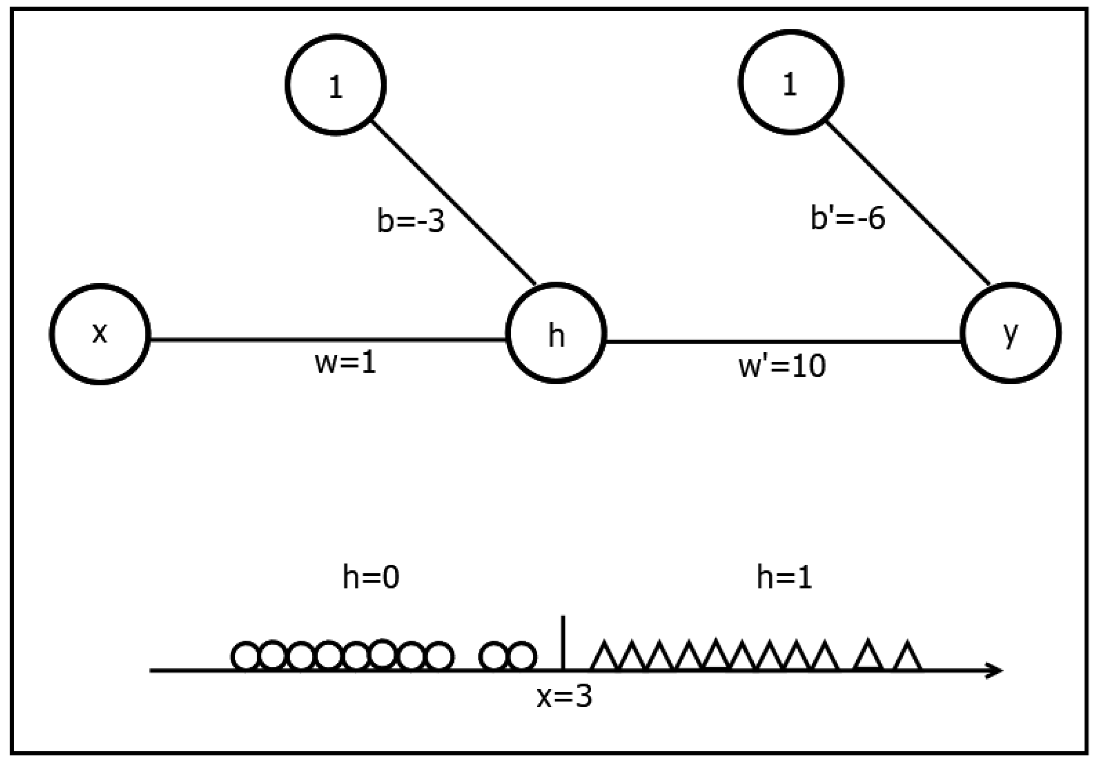
Figure 2.
Schematic representation of the global explainability for a DIMLP model. From a trained DIMLP the hyperplanes are precisely located from the weights of the first hidden layer; then, FidexGlo runs Fidex for all the training samples. Finally, by removing as many rules as possible, FidexGlo simplifies the rules generated by Fidex.
Figure 2.
Schematic representation of the global explainability for a DIMLP model. From a trained DIMLP the hyperplanes are precisely located from the weights of the first hidden layer; then, FidexGlo runs Fidex for all the training samples. Finally, by removing as many rules as possible, FidexGlo simplifies the rules generated by Fidex.

Figure 3.
An example of ruleset generated by FidexGlo applied to an ensemble of 25 DIMLPs with a single hidden layer.
Figure 3.
An example of ruleset generated by FidexGlo applied to an ensemble of 25 DIMLPs with a single hidden layer.
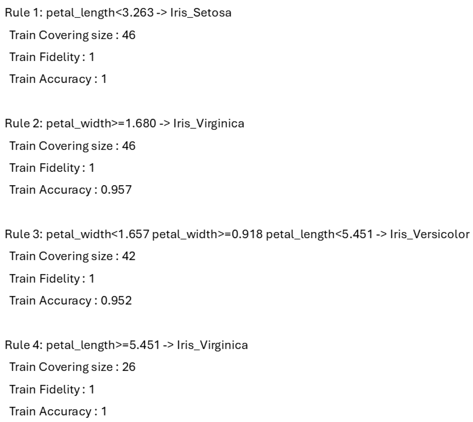
Figure 4.
An example of ruleset generated by FidexGlo applied to an ensemble of 100 DTs of depth three trained by gradient boosting.
Figure 4.
An example of ruleset generated by FidexGlo applied to an ensemble of 100 DTs of depth three trained by gradient boosting.
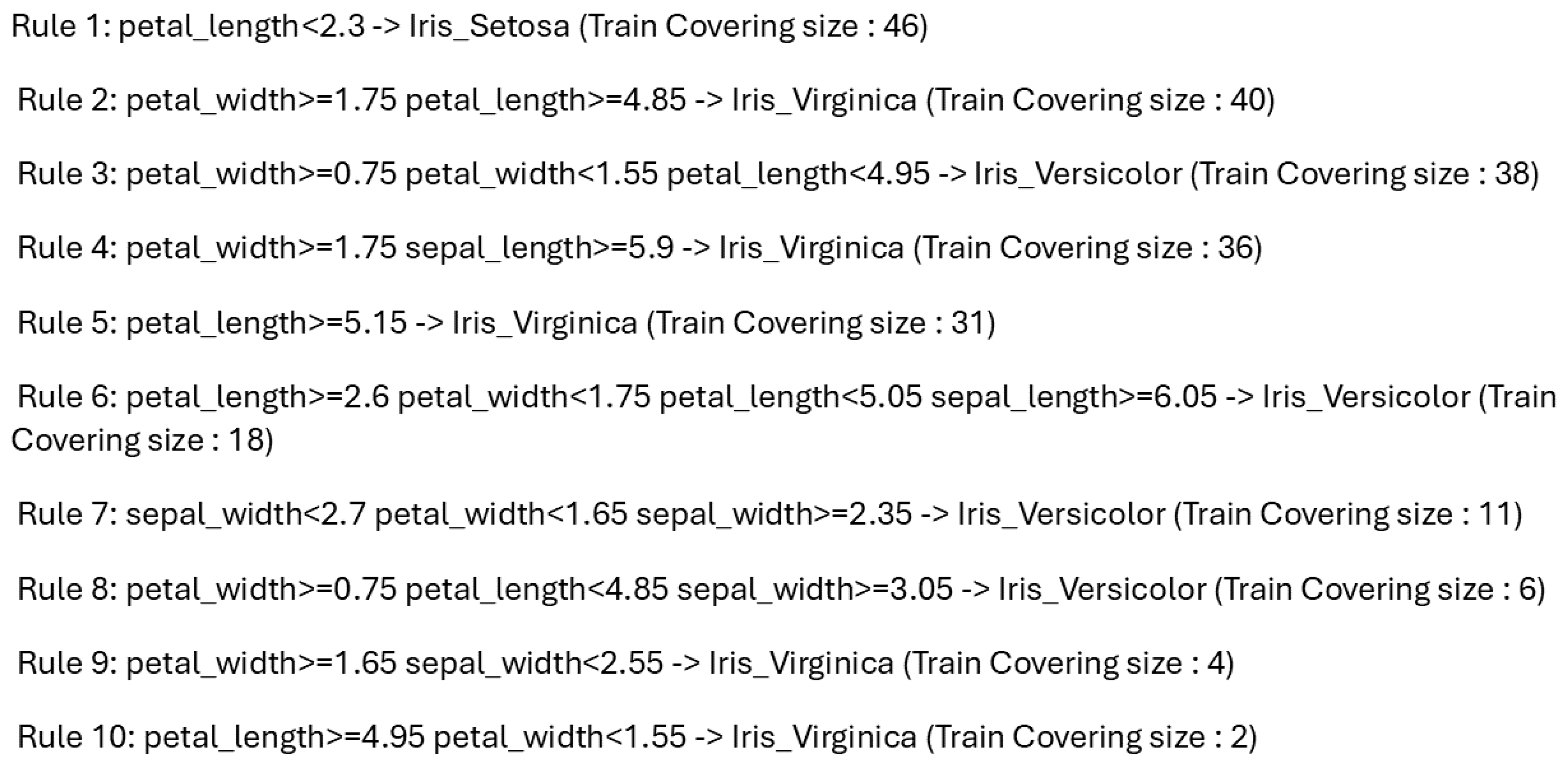
Figure 5.
Variation of the drop-out parameters (p and q) for the “Ionosphere” classification problem trained with DIMLP ensembles. The average number of rules is shown on the top left, the average number of antecedents per rule on the top right, the average fidelity on the bottom left, and the average prediction accuracy on the bottom right.
Figure 5.
Variation of the drop-out parameters (p and q) for the “Ionosphere” classification problem trained with DIMLP ensembles. The average number of rules is shown on the top left, the average number of antecedents per rule on the top right, the average fidelity on the bottom left, and the average prediction accuracy on the bottom right.
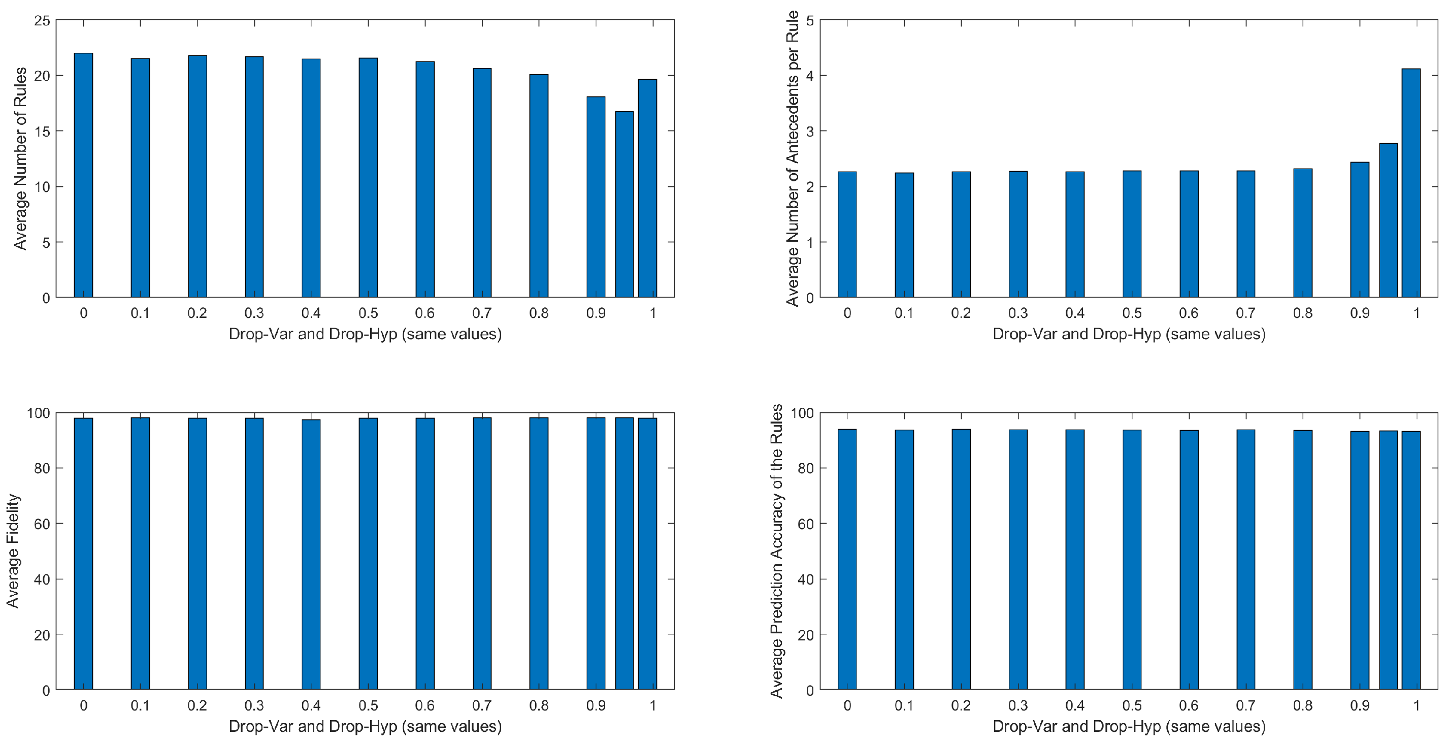
Figure 6.
Variation of the drop-out parameters (p and q) for the “Ionosphere” classification problem trained with Random Forests.
Figure 6.
Variation of the drop-out parameters (p and q) for the “Ionosphere” classification problem trained with Random Forests.
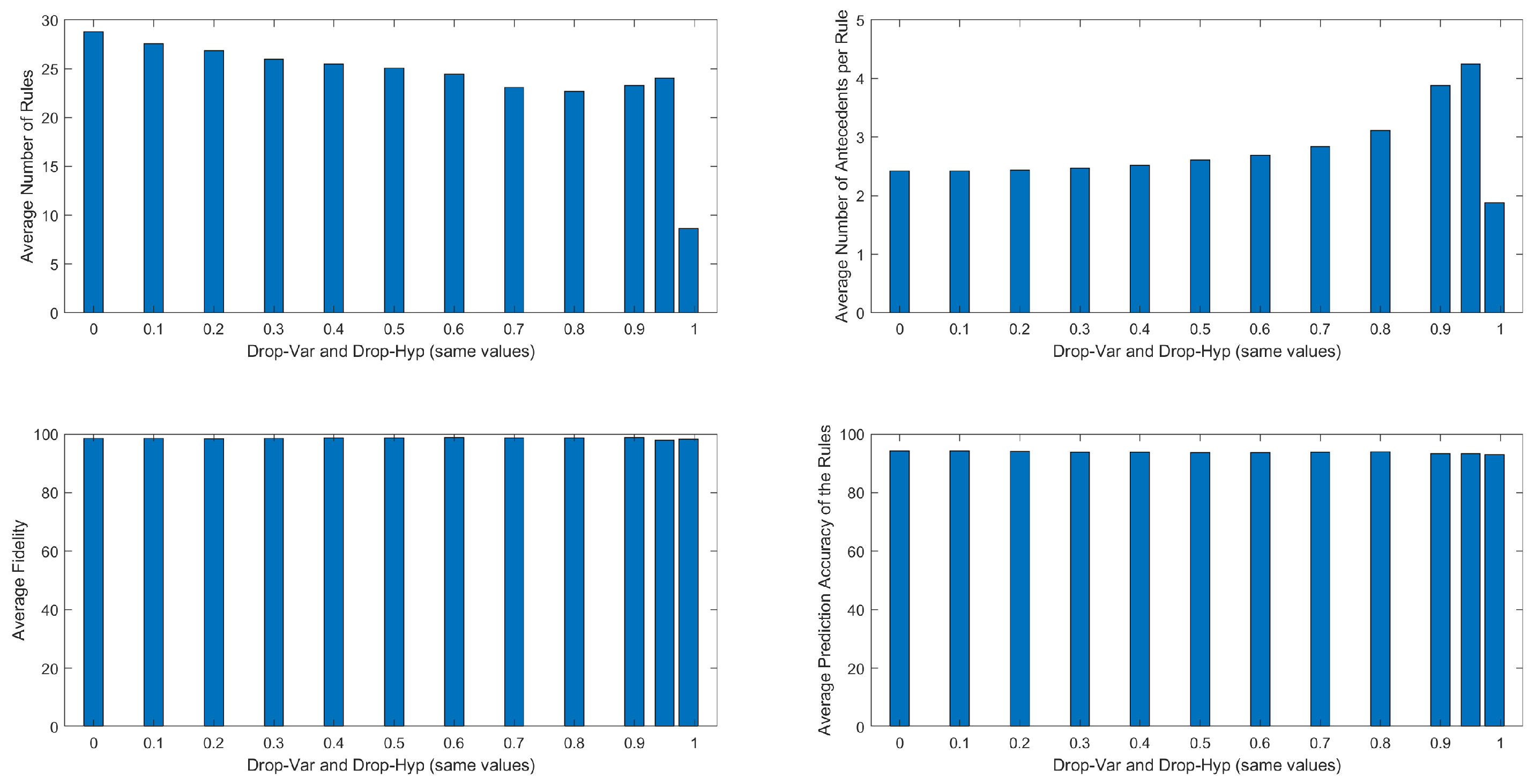
Figure 7.
Samples covered by a rule of class ’1’; rule antecedents are represented by colored dots. The top left shows the centroid of the 1426 covered samples in the training set, while the other pictures show three of the 242 samples in the test set that activate this rule.
Figure 7.
Samples covered by a rule of class ’1’; rule antecedents are represented by colored dots. The top left shows the centroid of the 1426 covered samples in the training set, while the other pictures show three of the 242 samples in the test set that activate this rule.
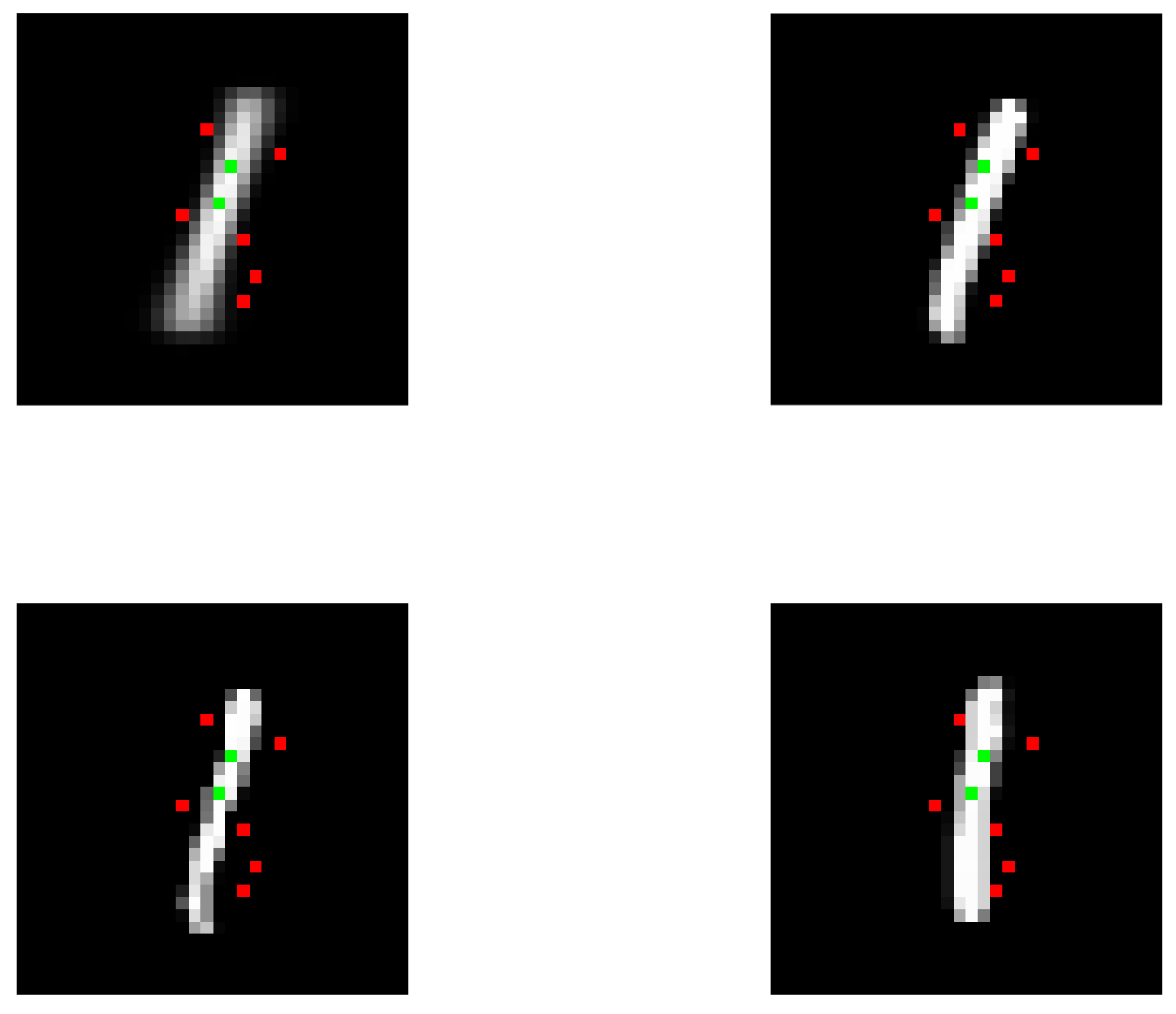
Figure 8.
Samples covered by a rule of class ’0’; rule antecedents are represented by colored dots. The top left shows the centroid of the 1114 covered samples in the training set, while the other pictures show three of the 183 samples in the test set that activate this rule.
Figure 8.
Samples covered by a rule of class ’0’; rule antecedents are represented by colored dots. The top left shows the centroid of the 1114 covered samples in the training set, while the other pictures show three of the 183 samples in the test set that activate this rule.
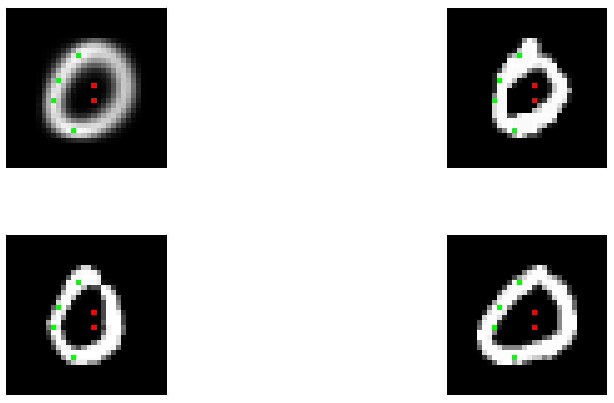
Figure 9.
Samples covered by a rule of class ’4’; rule antecedents are represented by colored dots. The top left shows the centroid of the 565 covered samples in the training set, while the other pictures show three of the 103 samples in the test set that activate this rule.
Figure 9.
Samples covered by a rule of class ’4’; rule antecedents are represented by colored dots. The top left shows the centroid of the 565 covered samples in the training set, while the other pictures show three of the 103 samples in the test set that activate this rule.
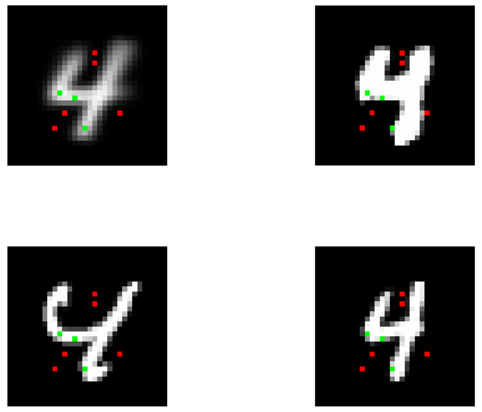
Figure 10.
Samples covered by a rule of class ’Happy’; rule antecedents are represented by colored dots. The top left shows the centroid of the 27 covered samples in the training set, while the other pictures show three of the eight samples in the test set that activate this rule.
Figure 10.
Samples covered by a rule of class ’Happy’; rule antecedents are represented by colored dots. The top left shows the centroid of the 27 covered samples in the training set, while the other pictures show three of the eight samples in the test set that activate this rule.
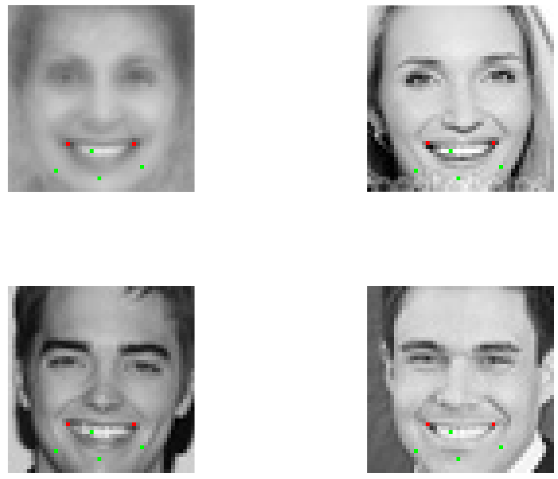
Figure 11.
Samples covered by a rule of class ’Happy’; rule antecedents are represented by colored dots. The top left shows the centroid of the 30 covered samples in the training set, while the other pictures show three of the six samples in the test set that activate this rule.
Figure 11.
Samples covered by a rule of class ’Happy’; rule antecedents are represented by colored dots. The top left shows the centroid of the 30 covered samples in the training set, while the other pictures show three of the six samples in the test set that activate this rule.
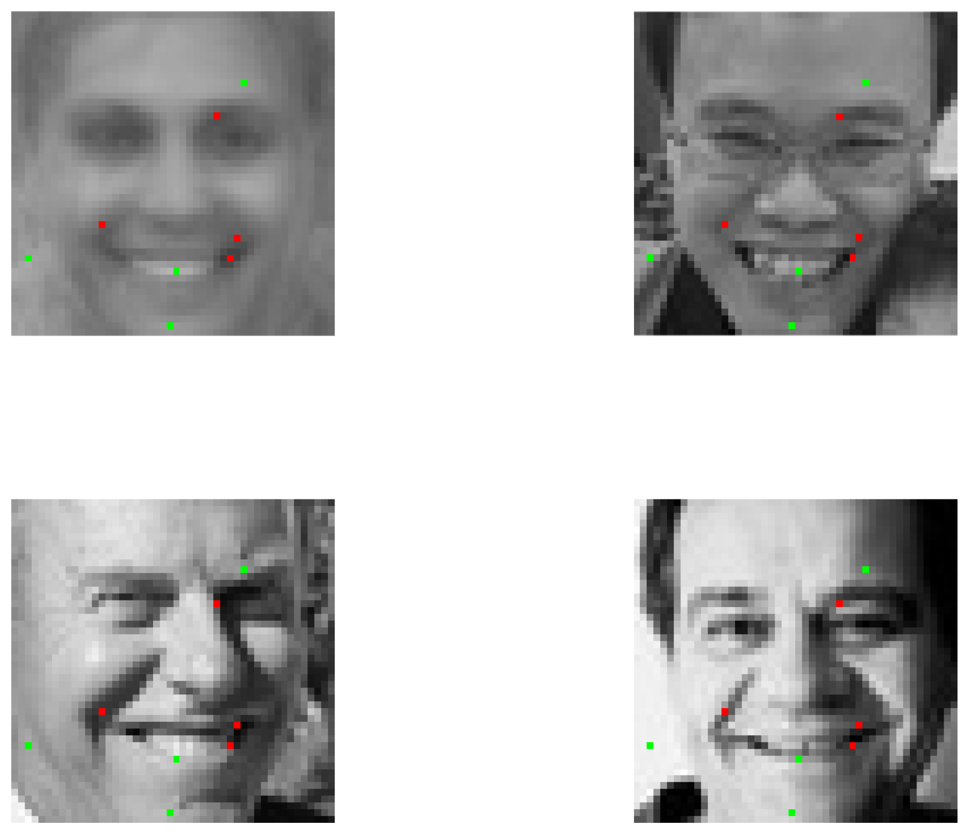
Figure 12.
Samples covered by a rule of class ’Happy’; rule antecedents are represented by colored dots. The top left shows the centroid of the 29 covered samples in the training set, while the other pictures show three of the eight samples in the test set that activate this rule.
Figure 12.
Samples covered by a rule of class ’Happy’; rule antecedents are represented by colored dots. The top left shows the centroid of the 29 covered samples in the training set, while the other pictures show three of the eight samples in the test set that activate this rule.
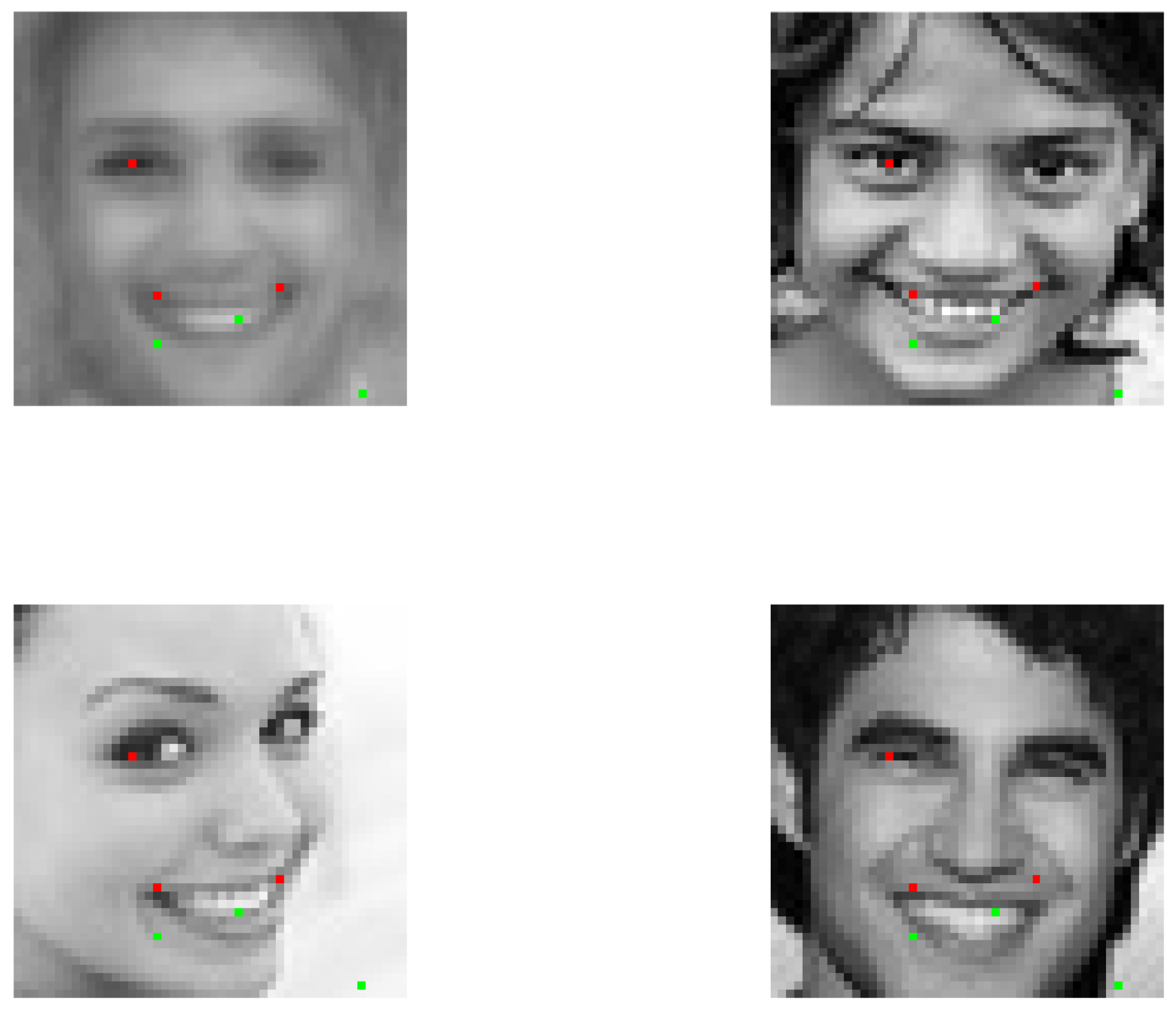
Figure 13.
Samples covered by a rule of class ’Cracks’; rule antecedents are represented by colored dots. The top left shows the centroid of the 4549 covered samples in the training set, while the other pictures show three of the 1120 samples in the test set that activate this rule.
Figure 13.
Samples covered by a rule of class ’Cracks’; rule antecedents are represented by colored dots. The top left shows the centroid of the 4549 covered samples in the training set, while the other pictures show three of the 1120 samples in the test set that activate this rule.
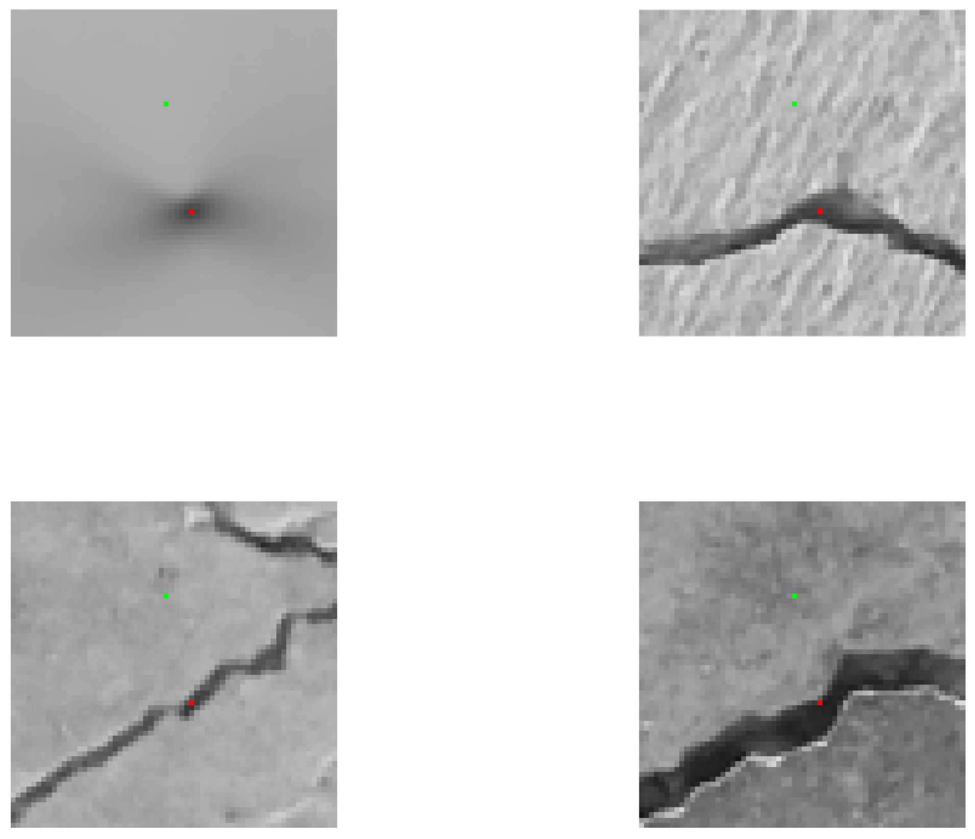
Figure 14.
Samples covered by a rule of class ’Cracks’; rule antecedents are represented by colored dots. The top left shows the centroid of the 4429 covered samples in the training set, while the other pictures show three of the 1070 samples in the test set that activate this rule.
Figure 14.
Samples covered by a rule of class ’Cracks’; rule antecedents are represented by colored dots. The top left shows the centroid of the 4429 covered samples in the training set, while the other pictures show three of the 1070 samples in the test set that activate this rule.
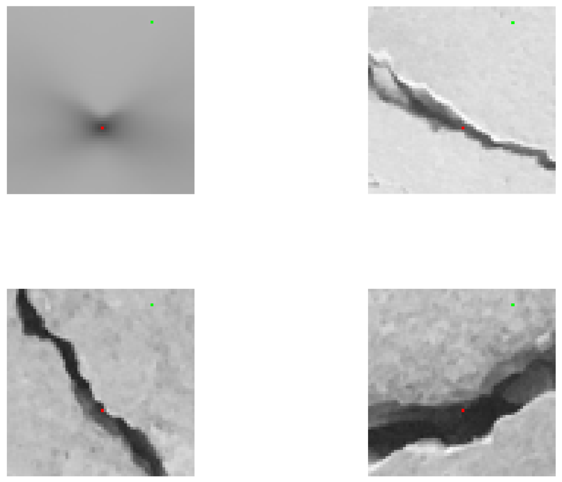

Table 1.
Datasets used in the experiments. From left to right, columns designate: number of samples; number of input features; type of features (boolean, categorical, integer, real); and proportion of samples in the majority class.
Table 1.
Datasets used in the experiments. From left to right, columns designate: number of samples; number of input features; type of features (boolean, categorical, integer, real); and proportion of samples in the majority class.
| Dataset | #Samp. | #Attr. | Attr. Types | Maj. Class (%) |
|---|---|---|---|---|
| Breast Cancer | 683 | 9 | int. | 65.0 |
| Divorce | 170 | 54 | bool. | 50.6 |
| Iris | 150 | 4 | real | 33.3 |
| Ionosphere | 351 | 34 | int., real | 64.1 |
Table 2.
Average results obtained on the “Iris” dataset by cross-validation.
| Model | Acc. | Fid. | Acc. R. (a) | Acc. R. (b) | Nb. R. | Nb. Ant. |
|---|---|---|---|---|---|---|
| DIMLP () | 94.9 (0.5) | 99.6 (0.5) | 95.3 (0.5) | 95.3 (0.5) | 4.5 (0.4) | 1.6 (0.1) |
| DIMLP () | 94.5 (0.6) | 99.5 (0.5) | 94.5 (0.8) | 94.7 (0.7) | 5.9 (0.6) | 1.9 (0.1) |
| RF () | 95.3 (0.5) | 99.5 (0.5) | 94.9 (0.5) | 95.3 (0.5) | 10.5 (0.3) | 2.4 (0.0) |
| RF (—) | 95.2 (0.8) | 99.1 (0.8) | 94.8 (0.5) | 95.4 (0.7) | 10.4 (0.2) | 2.4 (0.0) |
| GB () | 94.3 (0.6) | 99.8 (0.3) | 94.2 (0.5) | 94.3 (0.6) | 7.7 (0.4) | 2.3 (0.1) |
| GB () | 95.3 (0.4) | 99.5 (0.6) | 95.1 (0.6) | 95.5 (0.4) | 10.3 (0.3) | 2.4 (0.0) |
Table 3.
Average results obtained on the “Breast Cancer” dataset. The first row shows DIMLPs with only a single hidden layer, the second is DIMLP with ten neurons in the second hidden layer, then QSVM with the linear kernel, QSVM with the RBF kernel, RF with trees of depth ten, RF with unconstrained depth, GB with depth one and GB with depth three.
Table 3.
Average results obtained on the “Breast Cancer” dataset. The first row shows DIMLPs with only a single hidden layer, the second is DIMLP with ten neurons in the second hidden layer, then QSVM with the linear kernel, QSVM with the RBF kernel, RF with trees of depth ten, RF with unconstrained depth, GB with depth one and GB with depth three.
| Model | Acc. | Fid. | Acc. R. (a) | Acc. R. (b) | Nb. R. | Nb. Ant. |
|---|---|---|---|---|---|---|
| DIMLP () | 97.0 (0.1) | 99.4 (0.2) | 96.9 (0.2) | 97.2 (0.1) | 14.2 (0.4) | 2.2 (0.0) |
| DIMLP () | 97.2 (0.1) | 99.4 (0.2) | 97.3 (0.3) | 97.5 (0.2) | 14.3 (0.8) | 2.2 (0.0) |
| QSVM (lin.) | 97.1 (0.1) | 99.5 (0.1) | 97.2 (0.2) | 97.4 (0.2) | 14.8 (0.5) | 2.2 (0.0) |
| QSVM (RBF) | 97.1 (0.2) | 99.5 (0.3) | 97.1 (0.3) | 97.3 (0.2) | 14.2 (0.6) | 2.3 (0.0) |
| RF () | 97.1 (0.3) | 99.3 (0.2) | 96.8 (0.3) | 97.3 (0.4) | 29.0 (0.5) | 2.7 (0.0) |
| RF (—) | 97.2 (0.4) | 99.1 (0.3) | 96.8 (0.5) | 97.4 (0.5) | 28.9 (0.5) | 2.7 (0.0) |
| GB () | 96.5 (0.3) | 99.1 (0.3) | 96.6 (0.3) | 97.0 (0.2) | 15.1 (0.6) | 2.3 (0.0) |
| GB () | 97.0 (0.2) | 99.3 (0.2) | 96.6 (0.2) | 97.1 (0.2) | 28.6 (0.6) | 2.7 (0.0) |
| AdaC2 [35] | 92.4 (—) | — (—) | 95.6 (—) | — (—) | 10.8 (—) | — (—) |
| RF [13] | 97.4 (0.1) | 98.5 (0.2) | 96.9 (0.2) | 97.9 (0.2) | 24.3 (0.5) | 3.3 (0.0) |
| RuleFit [33] | — (—) | — (—) | 97 (2) | — (—) | 38 (5) | — (—) |
| SR [13] | — (—) | — (—) | 94.4 (0.2) | — (—) | 31.2 (1.7) | 2.7 (0.0) |
Table 4.
Average results obtained on the “Divorce” dataset.
| Model | Acc. | Fid. | Acc. R. (a) | Acc. R. (b) | Nb. R. | Nb. Ant. |
|---|---|---|---|---|---|---|
| DIMLP () | 98.2 (0.2) | 99.8 (0.3) | 98.0 (0.3) | 98.2 (0.2) | 6.6 (0.4) | 1.2 (0.0) |
| DIML () | 98.2 (0.0) | 99.6 (0.4) | 97.8 (0.0) | 98.2 (0.0) | 6.8 (0.3) | 1.2 (0.0) |
| QSVM (lin.) | 97.6 (0.0) | 99.8 (0.3) | 97.8 (0.3) | 97.8 (0.3) | 6.0 (0.3) | 1.2 (0.0) |
| QSVM (RBF) | 97.6 (0.0) | 99.5 (0.5) | 97.7 (0.3) | 97.9 (0.3) | 2.4 (0.2) | 1.0 (0.0) |
| RF () | 97.6 (0.0) | 99.8 (0.3) | 97.8 (0.3) | 97.8 (0.3) | 6.9 (0.3) | 1.2 (0.0) |
| RF (—) | 97.6 (0.0) | 99.9 (0.2) | 97.7 (0.2) | 97.7 (0.2) | 7.0 (0.3) | 1.2 (0.0) |
| GB () | 97.6 (0.0) | 99.8 (0.3) | 97.8 (0.4) | 97.8 (0.3) | 6.2 (0.3) | 1.4 (0.0) |
| GB () | 97.6 (0.0) | 99.9 (0.2) | 97.7 (0.2) | 97.7 (0.2) | 7.0 (0.2) | 1.2 (0.0) |
| GB [13] | 97.6 (1.1) | 99.5 (0.3) | 97.3 (1.0) | 97.7 (1.0) | 3.8 (0.0) | 1.5 (0.0) |
| SR [13] | — (—) | — (—) | 96.5 (0.7) | — (—) | 13.9 (1.0) | 2.7 (0.0) |
Table 5.
Average results obtained on the “Ionosphere” dataset.
| Model | Acc. | Fid. | Acc. R. (a) | Acc. R. (b) | Nb. R. | Nb. Ant. |
|---|---|---|---|---|---|---|
| DIMLP () | 92.8 (0.5) | 97.8 (0.6) | 93.8 (0.6) | 94.3 (0.4) | 21.2 (0.7) | 2.3 (0.0) |
| DIMLP () | 93.0 (0.7) | 97.9 (0.5) | 93.9 (0.9) | 94.4 (0.6) | 22.0 (1.0) | 2.3 (0.0) |
| QSVM (lin.) | 86.9 (0.7) | 95.8 (0.8) | 87.9 (0.6) | 89.1 (0.6) | 26.3 (1.3) | 2.5 (0.0) |
| QSVM (RBF) | 94.2 (0.5) | 97.3 (0.7) | 93.4 (0.5) | 95.0 (0.7) | 25.1 (0.9) | 2.5 (0.0) |
| RF () | 93.4 (0.5) | 98.5 (0.6) | 94.3 (0.6) | 94.5 (0.5) | 28.8 (0.8) | 2.4 (0.0) |
| RF (—) | 93.2 (0.2) | 98.5 (0.3) | 93.8 (0.6) | 94.1 (0.4) | 31.3 (0.5) | 2.5 (0.0) |
| GB () | 93.0 (0.5) | 98.3 (0.4) | 92.7 (0.6) | 93.6 (0.5) | 13.8 (0.5) | 2.5 (0.0) |
| GB () | 93.8 (0.4) | 98.9 (0.6) | 94.0 (0.4) | 94.4 (0.4) | 28.4 (0.8) | 2.5 (0.0) |
| AdaC2 [35] | 87.6 (—) | — (—) | 88.9 (—) | — (—) | 18.2 (—) | — (—) |
| DIMLP [13] | 93.0 (0.6) | 95.8 (0.8) | 92.3 (1.1) | 94.5 (0.6) | 18.3 (0.6) | 2.9 (0.1) |
| RuleFit [33] | — (—) | — (—) | 93 (5) | — (—) | 25 (3) | — (—) |
| SR [13] | — (—) | — (—) | 88.4 (0.8) | — (—) | 14.1 (0.9) | 3.0 (0.0) |
Table 6.
Average results provided by two CNN architectures with the MNIST dataset (ten trials). The first row designates the architecture described above and the second is a VGG architecture that was fine-tuned to this classification problem.
Table 6.
Average results provided by two CNN architectures with the MNIST dataset (ten trials). The first row designates the architecture described above and the second is a VGG architecture that was fine-tuned to this classification problem.
| Model | Acc. | Fid. | Acc. R. (a) | Acc. R. (b) | Nb. R. | Nb. Ant. |
|---|---|---|---|---|---|---|
| CNN-Small | 99.43 (0.06) | 96.43 (0.14) | 96.09 (0.16) | 99.58 (0.06) | 6082.1 (41.3) | 5.5 (0.0) |
| CNN-VGG | 99.47 (0.06) | 96.40 (0.20) | 96.10 (0.20) | 99.62 (0.04) | 6063.6 (33.6) | 5.6 (0.0) |
Table 7.
Average results provided of a CNN-VGG architecture on the FER dataset (ten trials). The results are related to a two-class problem: ’Happy’ versus ’Unhappy’.
Table 7.
Average results provided of a CNN-VGG architecture on the FER dataset (ten trials). The results are related to a two-class problem: ’Happy’ versus ’Unhappy’.
| Model | Acc. | Fid. | Acc. R. (a) | Acc. R. (b) | Nb. R. | Nb. Ant. |
|---|---|---|---|---|---|---|
| CNN-VGG | 90.81 (0.69) | 93.06 (0.67) | 86.21 (0.63) | 91.38 (0.93) | 6765.1 (72.4) | 4.4 (0.1) |
Table 8.
Average results of a CNN-VGG architecture on the Cracks dataset (ten trials). The results are related to a two-class problem: ’Cracks’ versus ’No-Cracks’.
Table 8.
Average results of a CNN-VGG architecture on the Cracks dataset (ten trials). The results are related to a two-class problem: ’Cracks’ versus ’No-Cracks’.
| Model | Acc. | Fid. | Acc. R. (a) | Acc. R. (b) | Nb. R. | Nb. Ant. |
|---|---|---|---|---|---|---|
| CNN-VGG | 99.86 (0.02) | 99.30 (0.11) | 99.21 (0.09) | 99.88 (0.02) | 1104.3 (37.7) | 14.2 (0.3) |
Disclaimer/Publisher’s Note: The statements, opinions and data contained in all publications are solely those of the individual author(s) and contributor(s) and not of MDPI and/or the editor(s). MDPI and/or the editor(s) disclaim responsibility for any injury to people or property resulting from any ideas, methods, instructions or products referred to in the content. |
© 2025 by the authors. Licensee MDPI, Basel, Switzerland. This article is an open access article distributed under the terms and conditions of the Creative Commons Attribution (CC BY) license (http://creativecommons.org/licenses/by/4.0/).
Copyright: This open access article is published under a Creative Commons CC BY 4.0 license, which permit the free download, distribution, and reuse, provided that the author and preprint are cited in any reuse.