Development of a MetUM (v 11.1) and NEMO (v 3.6) Coupled Operational Forecast Model for the Maritime Continent: Evaluation of Atmospheric Forecasts

1. Introduction

Atmospheric circulation and precipitation are strongly influenced by oceanic mean states and anomalies. Sea surface temperature (SST) anomalies play a key role in modifying surface wind patterns, atmospheric stability, and precipitation, significantly impacting global atmospheric circulation (Small et al., 2008; Chelton & Xie, 2010; Seo et al., 2014, 2019; Ma et al., 2016; Frolov et al., 2021). Large-scale SST anomalies drive diabatic heating or cooling in the atmosphere, which in turn modifies wind stress and heat fluxes at the ocean surface. These coupled air-sea interactions manifest both positive (Bjerknes, 1969; Xie and Philander, 1994) and negative (Ramanathan and Collins, 1991) feedback, contributing to the complexity of ocean-atmosphere coupling via SSTs. The strength of this coupling varies regionally, from the equator to the poles, with tropical regions exhibiting stronger dynamical coupling, as SSTs in these areas significantly influence wind stress and atmospheric circulation patterns.

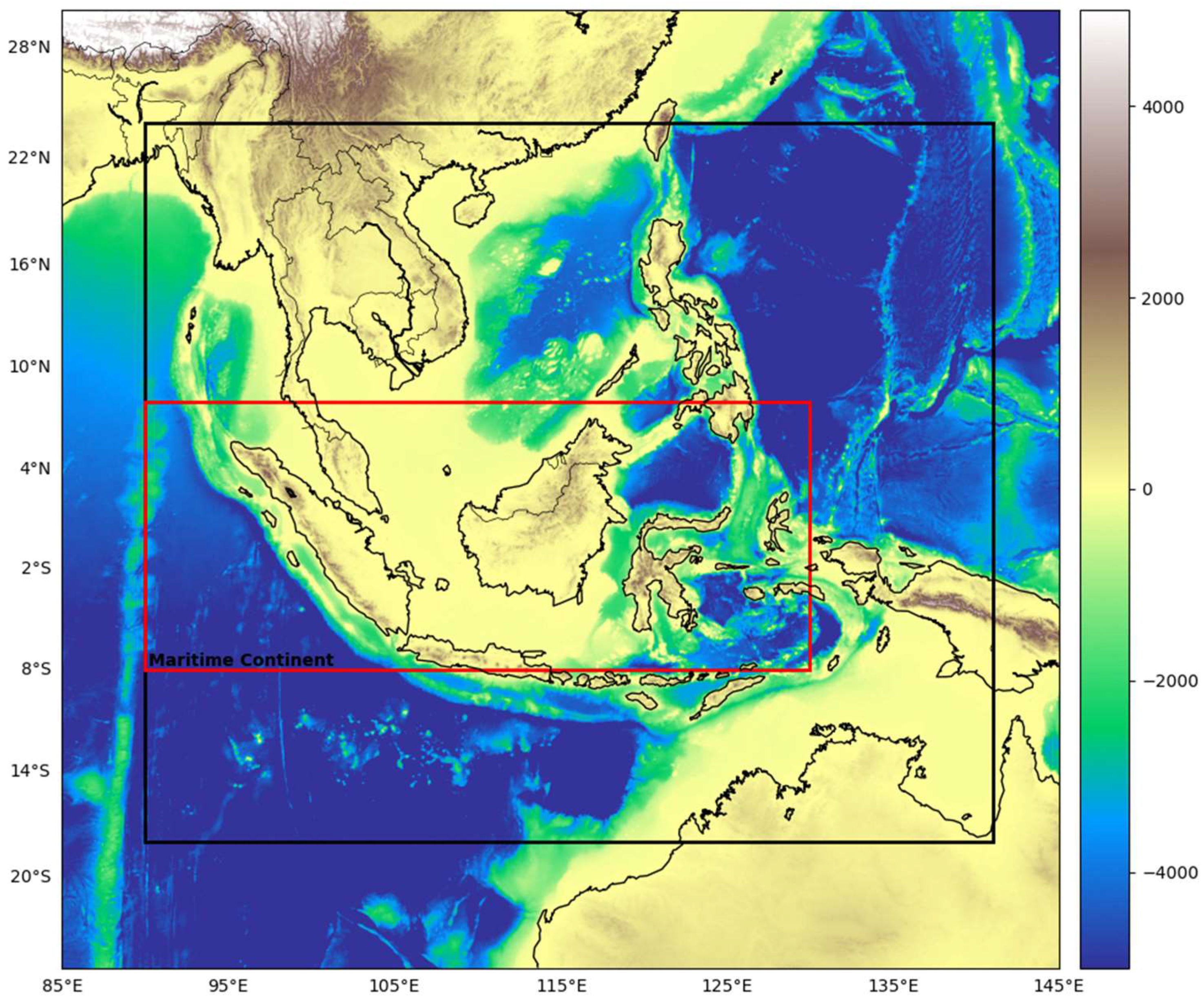
One such key region is the Maritime Continent (MC), situated between the Pacific and Indian Oceans, roughly bounded by 8°S–8°N, 90°–130°E (Ramage, 1968). The MC is composed of numerous islands including those within the Indonesian and Malay archipelagos and is characterized by complex geography and shallow seas. Located in the Indo-Pacific warm pool, the MC is a region of extensive moisture evaporation and intense rainfall, which makes it a critical source of latent heat for large-scale atmospheric circulation (Ramage, 1968; Gianotti et al., 2012; Krishnamurti et al., 1973; Yamanaka et al., 2018; Ruppert et al., 2019; 2020; Jiang and Li, 2018; Simpson et al., 1993; Neale and Slingo, 2003). Simulating rainfall over the Maritime Continent (MC) is particularly challenging due to the region's complex factors, including convection processes, coastal breezes, cloud cover, and varied land topography (Qian, 2008). The interplay between these factors affects rainfall patterns, making it difficult to accurately predict precipitation. Therefore, improving the representation of these processes in regional models is essential for enhancing weather forecasting and long-term climate projections. On the oceanic side, the MC is crucial due to its role as a low-latitude link between the tropical Pacific and Indian Ocean circulations via the Indonesian Throughflow (ITF) (Godfrey, 1996; Gordon et al., 2012; Qu et al., 2009; Lee et al., 2019; Xue et al., 2020). Therefore, accurate modeling of oceanic and atmospheric variables over the MC is necessary for a comprehensive understanding of both regional and global weather and climate dynamics.

Modeling atmospheric and oceanic variables over the MC presents challenges, particularly given the region’s intricate land-sea configuration and the presence of strong local mesoscale circulations. A significant portion of the MC is ocean-covered, making accurate representation of two-way air-sea feedback processes critical for improving weather and climate models. Models focusing solely on either the atmosphere or the ocean fail to fully capture the complex dynamics occurring at the ocean-atmosphere interface (Xue et al., 2020). Fully coupled atmosphere-ocean models are essential for simulating these interactions and the resulting surface dynamics (Xue et al., 2020). However, the effects of coupling the atmosphere and ocean models on precipitation remain a topic of ongoing research and debate. While coupling often leads to improvements in simulating sea surface temperature (SST) and air-sea heat fluxes, its impact on precipitation patterns is more variable. Some studies have shown that coupled models significantly enhance the accuracy of precipitation forecasts, whereas others report minimal or no improvements (Aldrian et al., 2005; Wei et al., 2014; Thompson et al., 2018). The disagreements between previous studies suggest that the benefits of coupling depend on factors such as model configuration, resolution, and the specific meteorological characteristics of the MC region. Higher resolution models tend to better simulate extreme rainfall events by capturing localized convection and orographic effects (Li et al., 2017; Dipankar et al., 2020).

The development of coupled atmosphere-ocean models at convective scale resolution has advanced significantly in recent decades, with applications extending to both research and operational forecasts. In high-resolution regional modeling, capturing convection scales is critical due to their strong influence on diurnal cycles and the offshore propagation of convective systems. Convection-resolving models allow for the direct representation of convective processes, which traditional parameterizations cannot accurately capture. This is essential for understanding and predicting phenomena like diurnal heating, which drives daily temperature fluctuations and storm development. Enhancing weather forecasts through coupled modeling systems is now recognized as a priority for further development (e.g., Lewis et al., 2019). However, despite advances, the prediction of atmospheric variables over the MC continues to involve a high degree of uncertainty, largely due to gaps in knowledge concerning the coupled system and its key drivers (Christensen et al., 2007; Xue et al., 2020). Previous studies have highlighted the necessity of incorporating coupled models to more accurately simulate atmospheric and oceanic variables over the MC (Thompson et al., 2018; Xue et al., 2020). This underscores the necessity to develop high-resolution coupled ocean-atmosphere models tailored specifically for the MC. The model development and preliminary assessment of ocean forecasts are detailed in Thompson et al. (2021). In this study, we evaluate the performance of the regional atmosphere-ocean coupled model with a focus on atmospheric forecast accuracy, validating against observations and reanalysis datasets. Section 2 provides an overview of the models, data, and methodologies used, while Section 3 discusses the results. We conclude with recommendations for further improvements in Section 4.

2. Models, Data, and Methodology

2.1. Models

This study employs a newly developed fully coupled atmosphere-ocean prediction system specifically designed for the Maritime Continent (MC) region. The model covers a domain extending from 90°E to 141°E and 18°S to 25.6°N (Figure 1), encompassing the tropical eastern Indian and western Pacific Oceans on a regular latitude-longitude grid. To avoid potential numerical instabilities from steep bathymetric features, such as the Mariana Trench, the eastern boundary is set at 141°E (Thompson et al., 2021). Both the atmospheric and oceanic components share this domain, for an easier coupling infrastructure with a horizontal resolution of 4.5 km. There are two experiments ran to assess the performance of the coupled system (i) the coupled system, refered as MCao, (ii) the atmosphere only version as MCa. Within the MCao configuration, the atmospheric and oceanic components are denoted MCAao and MCOao, respectively. Detailed descriptions of the atmosphere and ocean models are provided in the subsequent sections.

2.1.1. Atmospheric Model

The atmospheric component of both MCao and MCa utilizes the SINGV v5 science configuration (Huang et al. 2019; Dipankar et al., 2020), which closely resembles the RA1T (Regional Atmosphere v1 in the Tropics) configuration of the Met Office Unified Model (Bush et al., 2020). SINGV v5, described extensively by Huang et al. (2019), has been operational since 2019 at the Meteorological Service Singapore, running at a finer resolution (1.5 km) over the domain from 95°E to 109°E and 6°S to 7°N. Its dynamical core uses the non-hydrostatic semi-Lagrangian and semi-implicit ENDGAME system (Wood et al., 2014), operating on an Arakawa C-grid with a terrain-following vertical coordinate system. The model consists of 80 vertical levels, with high resolution near the surface (5 m spacing in the boundary layer) and a model top at 38.5 km. A model integration time step of 120 s is used to ensure the numerical stability.

The model incorporates the Prognostic Cloud fraction and Prognostic Condensate scheme (PC2; Wilson et al., 2008) and boundary layer parameterization is based on a hybrid approach by Boutle et al. (2014), combining the 1D scheme of Lock et al. (2001) with the 3D Smagorinsky-Lilly scheme (Lilly, 1962). The microphysics and radiation schemes are based on Wilson and Ballard (1999) and Edwards and Slingo (1996), respectively, with shortwave and longwave radiation divided into six and nine bands (Manners et al., 2011). The Joint UK Land Environment Simulator (JULES, Best et al., 2011) serves as the land surface scheme, offering nine surface fraction types. Further model formulations and scheme details are elaborated in Thomson et al. (2021).

2.1.2. Ocean Model

The ocean component of MCao is based on the regional Ocean PArallelise (OPA) engine within the NEMO framework (v3.6_stable, revision 6232; Madec et al., 2016). NEMO, a hydrostatic, Boussinesq model, is widely used for climate and operational forecasting. The model uses an orthogonal curvilinear grid with Arakawa C-grid staggering, and its bathymetry is derived from the General Bathymetric Chart of the Oceans (GEBCO) 2014 dataset (https://www.gebco.net/data_and_products/historical_data_sets/#gebco_2014, last access: 9 December 2020) at 30-arc-second resolution. The ocean model includes 51 vertical levels with a terrain-following (sigma) coordinate system, utilizing a stretching function by Siddorn and Furner (2013). The baroclinic and barotropic model time steps are set to 120 s and 8 s, respectively.

Vertical mixing is handled by the Generic Length Scale (GLS) turbulence model (Umlauf and Burchard, 2013), with additional mixing due to internal tide breaking (St. Laurent et al., 2002). Bottom drag is parameterized using a logarithmic layer, with drag coefficients ranging from 0.0001 to 0.15. Sea surface height (SSH) and barotropic velocities are subject to Flather boundary conditions (Flather, 1976), while tracers and baroclinic velocities use a flow relaxation scheme (FRS; Davies, 1976). Solar radiation penetration are modeled using the red–blue–green (RGB) scheme (Lengaigne et al., 2007). Further ocean model specifications are detailed by Thompson et al. (2021).

2.1.3. Coupled Configuration

Coupling between the atmosphere and ocean models is facilitated through the Ocean Atmosphere Sea ice Soil coupler (version 3.3), interfaced with the Model Coupling Toolkit (OASIS3-MCT) libraries (Valcke, 2013). The Earth System Modelling Framework (ESMF) regridding tools are leveraged to generate interpolation weights for remapping exchange fields (Craig et al., 2017). The exchange of fluxes between the models is carried out with an hourly frequency. The atmosphere model transmits non-solar heat flux, net shortwave radiation, precipitation, net evaporation, and zonal and meridional wind stress heat flux to the ocean model, receiving sea surface temperature (SST) and zonal and meridional surface current fields in return. Mean sea level pressure (MSLP) is excluded from the coupled exchange to avoid numerical issues, with external data from ECMWF instead supplying MSLP to the ocean model (Thompson et al., 2021).

2.2. Data and Methodology

The atmosphere-ocean coupled forecast model operated as a pre-operational forecast system, initialise daily and run for 120 hours, from 1 October 2019 to 15 November 2019. Both coupled (MCao) and atmosphere-only (MCa) simulations were performed for the same period to assess coupling impacts. The atmospheric model is driven at the boundaries by ECMWF (European Centre for Medium Range Forecast) IFS (Integrated Forecast System) forecasts, a medium-range global weather prediction system available up to 10 d at a horizontal resolution of 0.1^∘ (https://www.ecmwf.int/en/forecasts/datasets/). Lateral boundaries for the Ocean model are driven by daily Mercator forecast (https://marine.copernicus.eu/). It is a global ocean reanalysis and forecast product based on NEMO v3.1 forced by the ECMWF IFS meteorological variables, provides oceanic variables with 0.0833^∘ horizontal resolution (Lellouche et al., 2018). While no spin-up was required for the atmospheric model due to sub-daily adjustments, a 5-year spin-up was performed for the ocean model (Thompson et al., 2021). This comprehensive setup ensured that the MCao model was initialized with accurate and reliable oceanic conditions, optimizing the performance and predictive capabilities of the coupled system. Tidal boundary conditions for the ocean model are provided by the Finite Element Solutions (FES2014b) dataset, a global finite-element mesh with increasing resolution in coastal and shallow waters regions (Lyard et al., 2006), incorporating 15 major tidal constituents (Q1, O1, P1, S1, K1, 2N2, Mu2, Nu2, N2, M2, L2, T2, S2, K2, and M4). The database is produced by assimilating long-term altimetry data and tidal gauges, distributed on a global 0.0625x0.0625 grid (http://www.aviso.altimetry.fr/en/data/products/auxiliary-products/global-tide-fes.html). Monthly runoff climatology from Dai and Trenberth (2002) and chlorophyll data from SeaWiFS satellite observations are used for runoff forcing and to compute light absorption coefficients in the ocean model respectively. In the coupled system, the MCAao is initialized daily at 00:00 UTC using ECMWF IFS analysis, while MCOao receives initial conditions from the previous day's simulation (T0 minus 1), driven by 6-hourly ECMWF IFS surface analysis and daily-mean Mercator Ocean forecasts at the lateral boundary. The MCao forecast run is driven by LBC from 3-hourly ECMWF IFS forecasts in the atmosphere and daily Mercator forecasts in the ocean. Since MSLP is not exchanged between MCAao and MCOao, 3-hourly ECMWF IFS forecast data are provided to MCOao. Both MCao and MCa forecast runs cover a 45-day period with a forecast lead time of 6 days.

To quantify the accuracy of precipitation forecasts, we used the Fractions Skill Score (FSS), a diagnostic tool that measures the spatial accuracy of forecasted rainfall relative to observed rainfall (Roberts and Lean, 2008). It is a neighborhood verification method commonly used by operational centres to verify high-resolution precipitation forecasts against observations (Mittermaier, 2021). FSS is particularly useful for assessing forecast skill at different scales, ranging from localized weather phenomena to broader regional trends. FSS scores range from 0 (indicating no skill) to 1 (indicating perfect skill), providing a clear measure of model performance. For the 10 m winds and 2 m air temperature, model evaluation was performed by computing the Mean Error (ME) and Root Mean Square Error (RMSE) between forecasted and observed parameters. The ocean model (MCOao) performance has been extensively evaluated in Thompson et al. (2021).

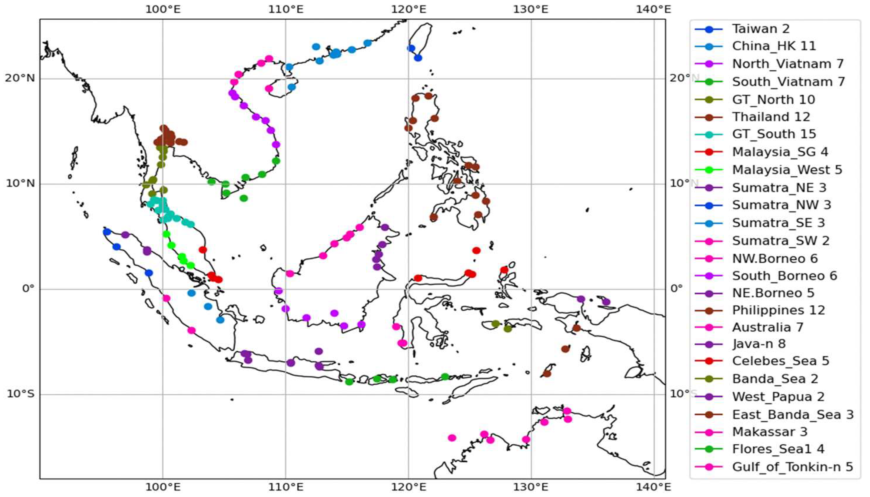
Validation data include the ERA5 reanalysis for 10 m winds (Herbach et al. 2020). Precipitation is compared against Integrated Multi-Satellite Retrievals for Global Precipitation Measurement (IMERG-GPM, abb. as GPM, Hou et al 2014). 10 m winds and 2 m temperature are validated against WMO land stations included in the MetDB database (MetOffice 2008). The locations of the WMO stations used in this study are shown in Figure 2. As the SST varies with latitude, to better understand its impact, we divided our analysis region on three latitude bands: (1) South of the equator up to 10°S, (2) North of the equator up to 10°N, and (3) regions outside the 10°S–10°N latitude band.

3. Results and Discussion

In this section, we assess the performance of the newly developed fully coupled atmosphere-ocean forecast model for the MC. We also illustrate the benefits of ocean-atmosphere coupling by comparing the predictive skill of the coupled model (MCao) with the standalone atmospheric model (MCa) across key meteorological parameters like precipitation, wind, and air temperature.

3.1. Precipitation

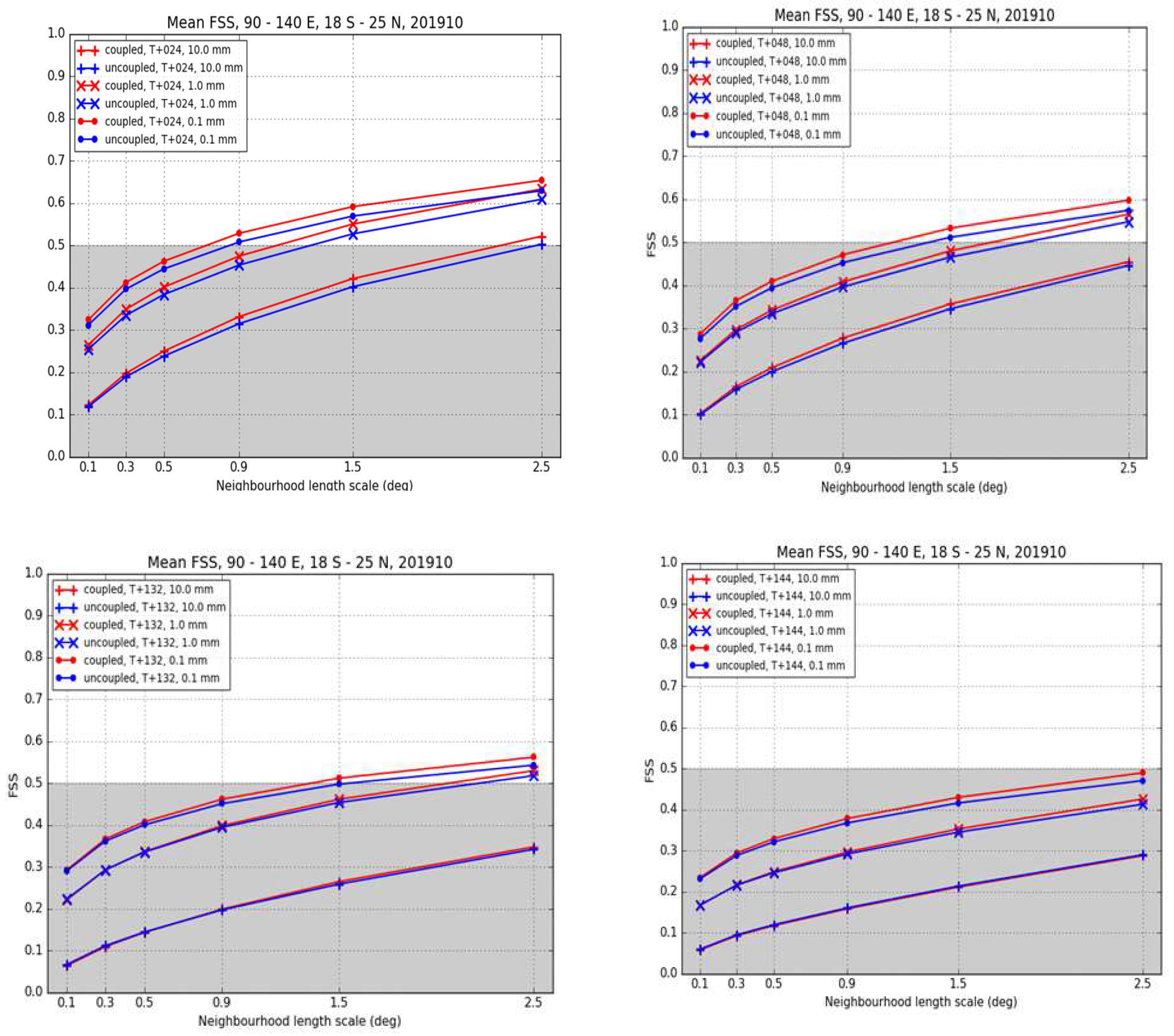
We calculated the precipitation FSS for both the coupled (MCao) and uncoupled (MCa) models over the full model domain (excluding points near the lateral boundaries). We focused on three-hourly accumulated rainfall data for the period from 1st to 31st October 2019, using different forecast lead times (T+24, T+48, T+132, and T+144) and rainfall thresholds (0.1, 1.0, and 10 mm/hr). The FSS vs. scale plots (Figure 2) show that the coupled model performs noticeably better than the uncoupled model at T+24 and T+48. The coupled model (MCao) consistently outperforms the standalone atmospheric model (MCa), particularly at T+24 and T+48 lead times, across all three precipitation thresholds. The difference in FSS scores between the two models becomes less pronounced as the forecast lead time increases. At the longer forecast ranges (T+132 and T+144), the coupled model performs slightly better at lower rainfall thresholds.

There is also a scale dependence: the FSS of the coupled model increases more with neighborhood length scale than that of the uncoupled model. At the lowest threshold of 0.1 mm/hr, corresponding to light rainfall, the MCao model demonstrates better forecast skill, as indicated by the higher FSS. These improvements are also observed at the 1.0 mm/hr threshold, representing moderate rainfall, though the margin of improvement is slightly smaller. At the higher threshold of 10 mm/hr, corresponding to heavy rainfall, the coupled model still outperforms the uncoupled model; however, the difference in FSS between MCao and MCa is less pronounced. This suggests that while ocean-atmosphere coupling improves forecasts for light and moderate rainfall, its impact on predicting heavy rainfall events is more limited. The forecast skill for heavy precipitation may be influenced by other factors, such as model resolution, convective parameterization, and the representation of sub-grid scale processes.

3.2. Wind

3.2.1. Qualitative Assessment: Typhoon Nakri Case Study

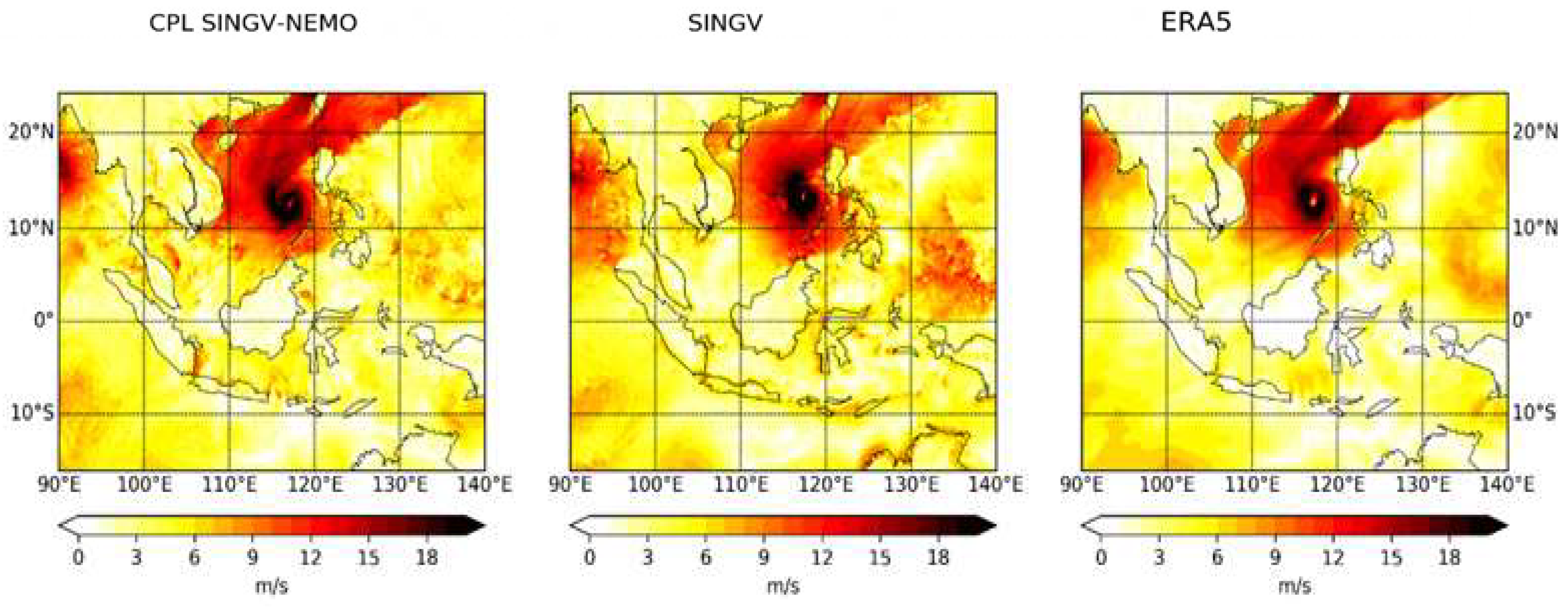
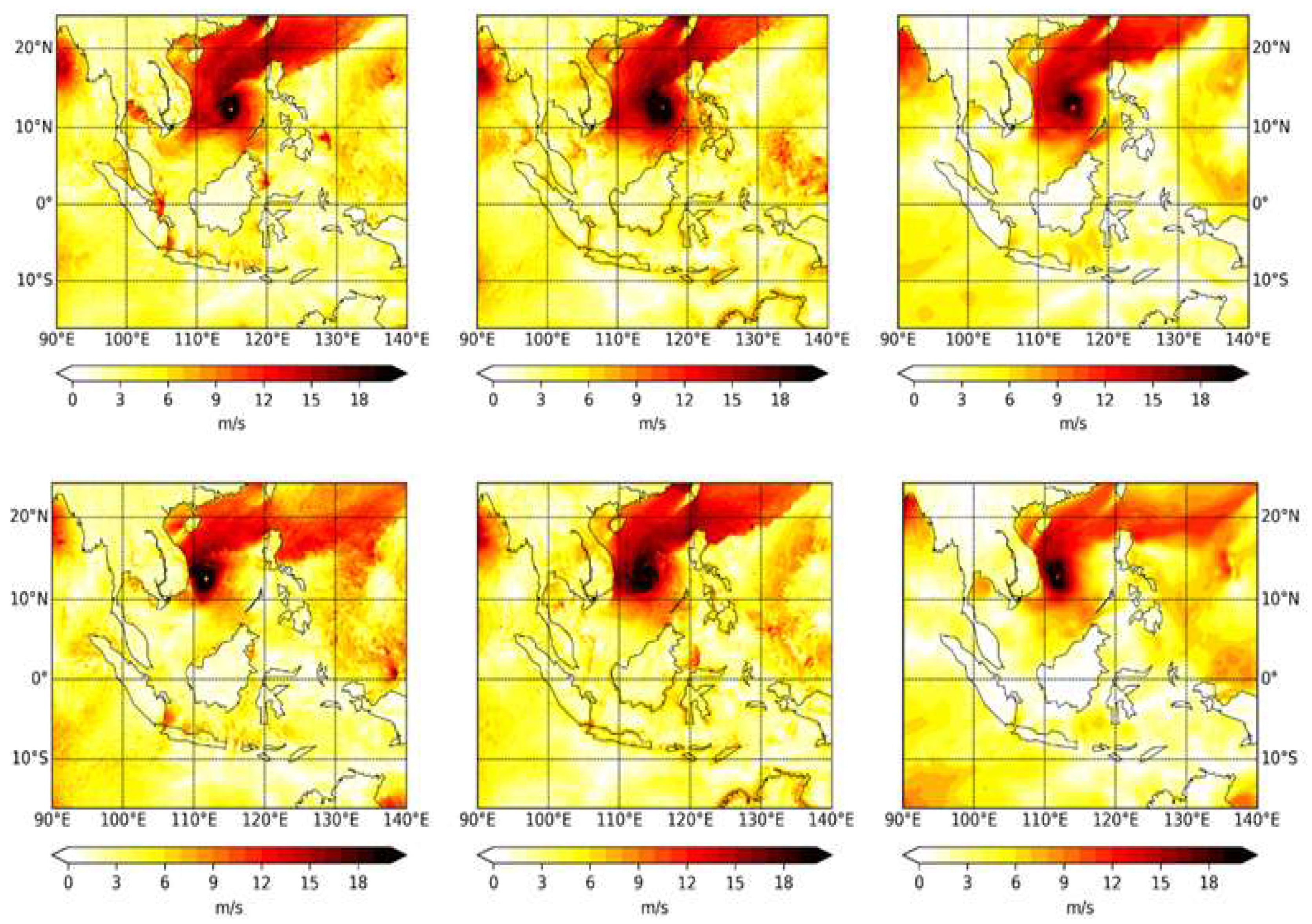
To assess the performance of the MCao model in simulating extreme wind conditions, we conducted a case study on Typhoon Nakri, which occurred in the South China Sea from November 4 to November 11, 2019. This typhoon provided an excellent opportunity to assess the effectiveness of the coupled atmosphere-ocean model in handling the complexities of extreme weather events. Typhoons, by nature, involve intricate interactions between the atmosphere and ocean, making them an ideal case for testing the benefits of coupling these systems.

In this study, we compared the spatial distribution of wind speeds simulated by the MCao and MCa models with ERA5 reanalysis data. ERA5 is widely regarded as one of the most accurate and reliable sources for atmospheric conditions, serving as a benchmark for model validation. To carry out the analysis, we focused on the forecast initialized at 00:00 UTC on November 6, which provided a snapshot of the typhoon's evolution at lead times: T+48 hours (November 8), T+72 hours (November 9), and T+96 hours (November 10) after initialization. Wind speeds at 10 meters above sea level were analyzed at these time points to evaluate the accuracy of the models' simulated wind fields (Figure 3).

The results from the case study indicate that the MCao model exhibited better performance in simulating the wind patterns and intensities associated with Typhoon Nakri when compared to the standalone MCa model. At the T+96 lead time, for example, the MCa model overestimated wind speeds in the vicinity of the typhoon (Figure 4). Such overestimations can lead to erroneous assessments of the typhoon’s intensity and potential impact, which could have serious implications for disaster preparedness, evacuation strategies, and emergency response. In contrast, the MCao model demonstrated a much closer alignment with the ERA5 data, especially in the core of the typhoon and its surrounding wind field. This closer alignment suggests that the two-way coupling between the atmosphere and ocean in the MCao model enhances its ability to capture the complex dynamics of the storm.

The improved performance of the MCao model can be attributed to the two-way interaction between the atmosphere and ocean, a key feature of coupled models. This coupling allows the model to more accurately simulate the exchange of energy, momentum, and moisture between the two systems, which plays a vital role in determining the intensity and structure of tropical cyclones. During extreme weather events like typhoons, feedback mechanisms between the ocean and atmosphere are especially important because they can either intensify or weaken the storm. For instance, the sea surface temperature can influence the storm’s intensity, while the storm’s winds can alter the ocean’s upper layers. By accounting for these interactions, the MCao model provides a more realistic representation of the typhoon’s behavior, leading to more accurate forecasts.

This case study of Typhoon Nakri underscores the significant advantages of incorporating ocean-atmosphere coupling into regional climate models. The findings emphasize that coupled models, like MCao, are crucial for improving the accuracy of wind forecasts, particularly in the context of tropical cyclones, where the dynamic interaction between the ocean and atmosphere is paramount. As tropical cyclones are among the most destructive natural disasters, enhancing the precision of their forecasts has far-reaching implications for risk management, disaster preparedness, and mitigation strategies.

Furthermore, a more detailed analysis examining the impact of ocean-atmosphere coupling on other aspects of the typhoon’s behavior—such as its track, intensity, and forecast skill—will be the focus of future research. This will provide deeper insights into how coupled models can be further optimized to enhance our predictive capabilities and contribute to more effective disaster response and resilience planning.

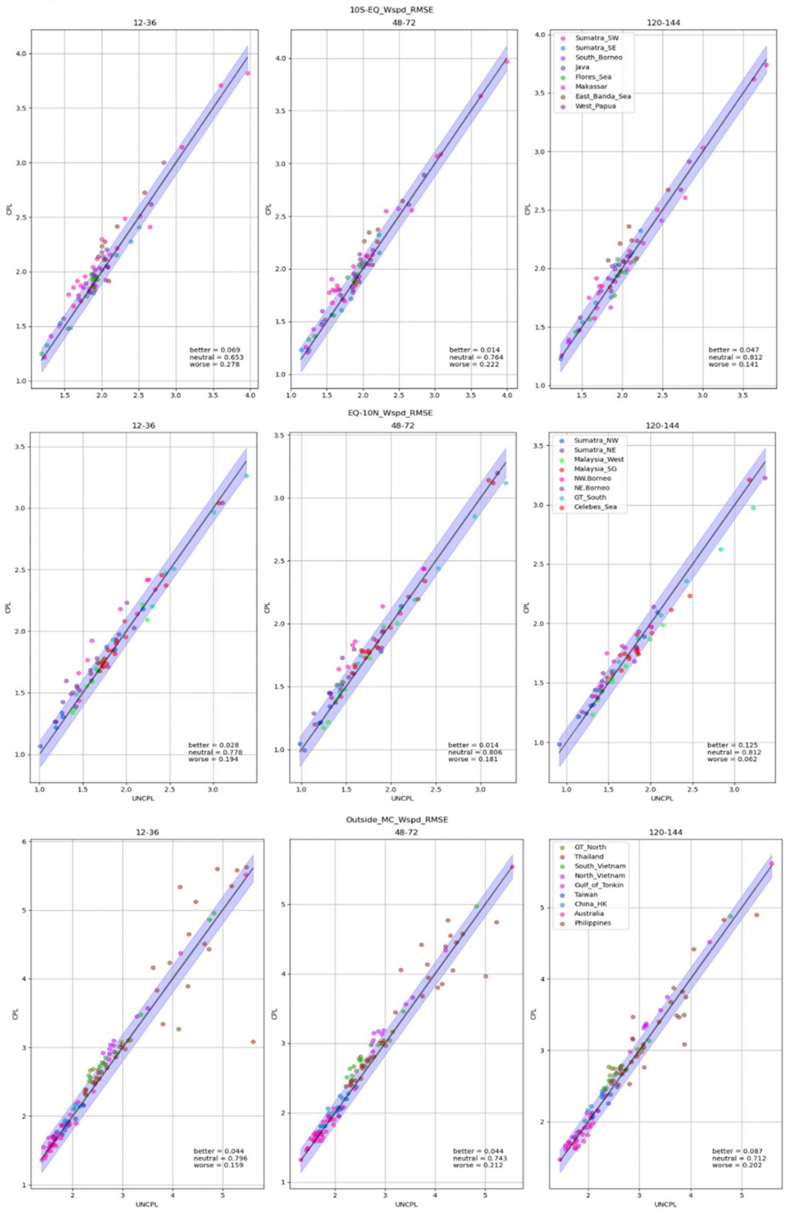
3.2.2. Verification Against WMO Stations

The performance of wind speed forecasts from the MCao and MCa models was evaluated using wind speed observations from WMO meteorological stations (Figure 2) for the period 1^st to 31^st of October. The Root Mean Square Error (RMSE) analysis of 10 m wind speed reveals the comparative performance of MCAao and MCa models across different regions: 10°S–Equator, Equator–10°N, and areas outside the Maritime Continent (MC), evaluated at three lead times (12–36, 48–72, and 120–144 hours) (Figure 5).

In the 10°S–Equator region (Figure 5 and Figure S1), MCAao provides only slight improvements over MCa. At shorter lead times (12–36 hours), the percentage of cases in the “better” category is relatively low (6.9%), while the majority of data points fall into the “neutral” category (72.8%), indicating comparable performance between the two models for most sub-regions. At longer lead times (48–72 and 120–144 hours), MCAao’s performance remains consistent, with minimal shifts in the distribution of “better” and “worse” cases (Figure 5). Regions such as Flores Sea, Makassar show minor benefits from MCAao, but these improvements are marginal (Figure S1). RMSE analysis revealed that most stations displayed neutral performance when comparing the coupled and uncoupled models (Figure S1). However, ME analysis highlighted subtle differences, with regions such as Java, the Banda Sea, and southwest Sumatra exhibiting slight improvements in the MCao model. Among the 43 stations in this region, 32% showed improved performance with the coupled model, while the remaining stations showed no significant difference (Figure S1).

For the Equator–10°N region (Figure 5 and Figure S2), MCAao exhibits slightly better performance compared to MCa, particularly at longer lead times (120–144 hours), where 12.5% of cases show improvement, compared to MCa (6.2%) (Figure 5). However, a significant portion of data points remains in the “neutral” category (81.2%), suggesting minimal differentiation between the models for most sub-regions, including Malaysia, Northern Borneo, and the Celebes Sea (Figure S2). A more detailed regional analysis revealed specific biases in wind speed forecasts. In northeastern Sumatra, the MCao model showed a positive bias during nighttime, leading to an overestimation of wind speeds, while during the day, a negative bias resulted in underestimations. In comparison, the MCa model exhibited smaller biases and thus performed slightly better in this region. In northwestern Sumatra, both models slightly overestimated daytime wind speeds, although the MCao model improved after the T+48 forecast lead time (Figure S2). Similarly, in the Celebes Sea, the MCao model initially overestimated wind speeds but showed improved accuracy for longer lead times, likely due to enhanced ocean-atmosphere interactions over extended simulation periods. In the Malaya Peninsula regions (Malaysia_SG and Malaysia_West), the MCao model outperformed the MCa model. Overall, among the 46 stations in the northern regions, 20% showed improvements with the MCao model, 13% favored the MCa model, and the remaining 67% displayed neutral performance (Figure S2).

In the regions outside the MC, MCao performance is mixed, with the MCa model generally showing better results in most regions (Figure 5 and Figure S3), whereas MCAao provides limited improvements in RMSE, with performance gains becoming more noticeable at longer lead times (120–144 hours). For shorter lead times (12–36 hours), MCAao’s improvements are negligible, with only 4.4% of cases falling into the “better” category. At 120–144 hours, MCAao achieves a slightly higher proportion of “better” cases (8.7%), though the improvements remain regionally dependent (Figure 5). Along the Vietnam coast and the northern region of the Gulf of Thailand, the MCao model slightly overestimated wind speeds compared to the MCa model. A similar overestimation is also observed in the China_HK region, which may be attributed to the enhanced ocean-atmosphere interactions in the coupled system. However, in stations around Australia, the MCao model demonstrated less bias compared to the MCa model. Among the 73 stations in this region, 57% displayed neutral performance, 34% showed better results with the MCa model, and 9% indicated improved performance with the MCao model.

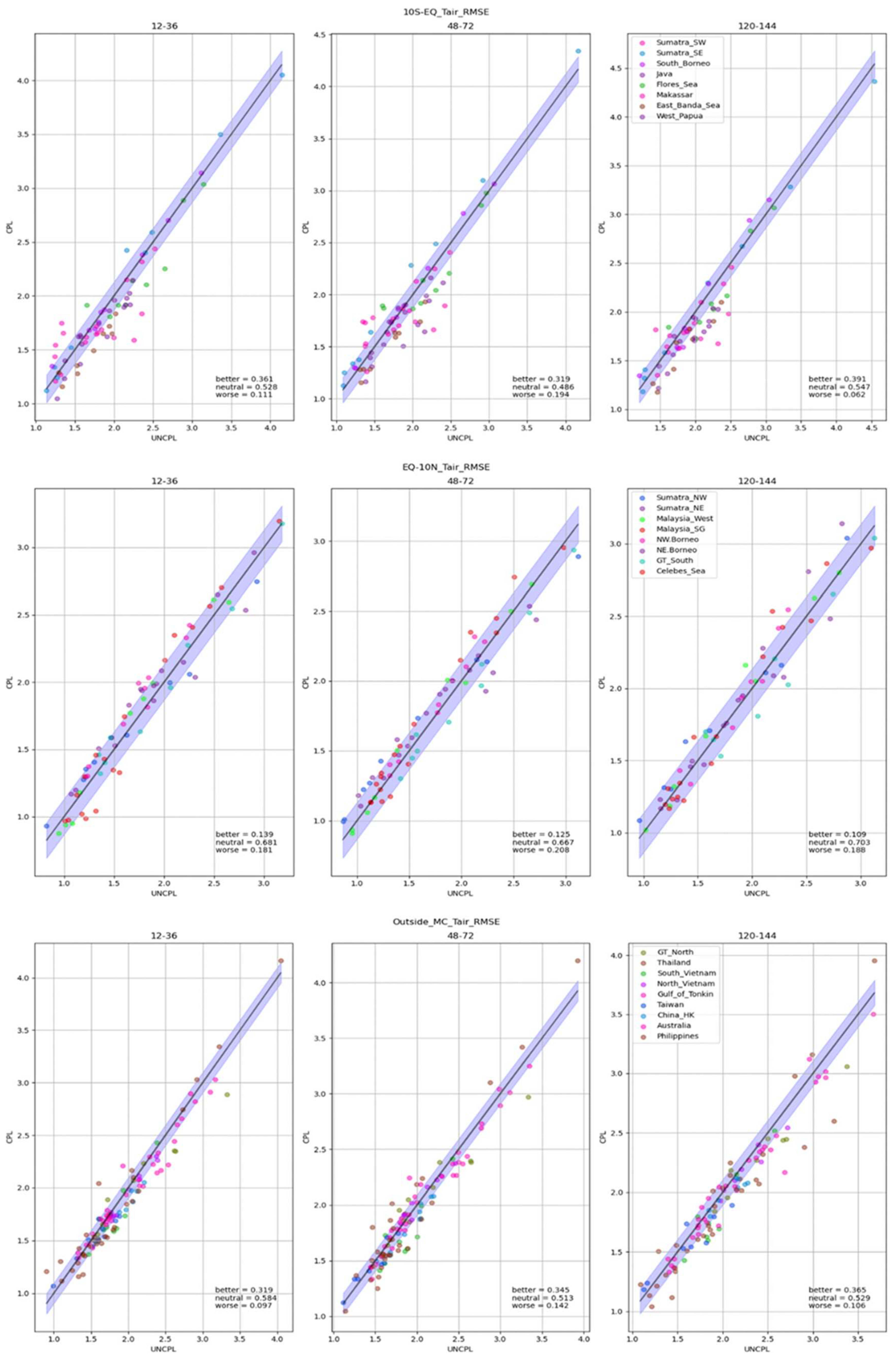
3.3. Air Temperature

In addition to wind speed analysis, we performed a quantitative evaluation of 2 m air temperature (Tair) forecasts from the MCao and MCa models and assessed utilizing Mean Error (ME) and Root Mean Square Error (RMSE) metrics, comparing model outputs against observations from WMO meteorological stations (Figure 6 and Figure S4–S6). The Root Mean Square Error (RMSE) analysis of Tair simulations highlights the enhanced performance of the MCAao model compared to the MCa model across different regions, including 10°S–Equator, Equator–10°N, and areas outside MC. Across all lead times (12–36, 48–72, and 120–144 hours), MCAao demonstrates a clear improvement in accuracy, as evidenced by most data points falling below the 1:1 line on the scatter plots, indicating reduced RMSE values relative to MCa.

In the 10°S–Equator region (Figure 6; Figure S4), MCAao shows substantial improvements, particularly at longer lead times (120–144 hours), where the model captures temperature variations more accurately. The percentage of cases categorized as “better” (cpl better than uncpl) is notably higher, while cases in the “neutral” and “worse” categories are minimal. Notably, regions such as southwest Sumatra (Sumatra_SW), Java, West Papua (West_Papua), the Banda Sea (East_Banda_Sea), and Makassar saw significant improvements in air temperature forecasts, show MCao’s ability to better resolve local air-sea interactions and diurnal temperature variations. In contrast, regions like southeast Sumatra (Sumatra_SE) and South Borneo showed no notable difference between the coupled and uncoupled models (Figure S4). Out of 43 stations in the southern regions, 79% displayed enhanced performance with the coupled model, while the remainder exhibited no obvious difference.

For the Equator–10°N region (Figure 6; Figure S5), RMSE indicates no significant difference between the two models at most stations. However, slight improvements were observed for the MCao model in the northeast Sumatra (Sumatra_NE) (Figure S5). Regarding ME, areas such as western Malaysia (Malaysia_West), Singapore (Malaysia_SG), northeastern Borneo (NE_Borneo), and the southern part of the Gulf of Thailand (GT_South) exhibited a slight advantage for the coupled model, particularly at longer lead times, highlighting the significance of ocean coupling (Figure S5). Among the 46 stations in this region, 70% reported improved performance with the coupled model, while 20% indicated better results with the uncoupled model, and 10% showed no substantial difference.

In areas outside the MC (Figure 6; Figure S6), MCao exhibits better performance, despite the greater variability in observational conditions and broader geographical extent. At medium- and long-range lead times, MCao achieves significant RMSE reductions, provides better overall predictions compared to MCa, with fewer cases in the “worse” category. Regions including northern Gulf of Thailand (GT_North), South Vietnam, and the Philippines experienced consistent improvements in temperature forecasts (Figure S6). Other areas, such as North Vietnam, the Gulf of Tonkin, Taiwan, China, Hong Kong, and Australia, also demonstrated slight improvements with the coupled model. Of the 73 stations in this region, 74% showed enhanced forecast accuracy with the coupled model, while the remainder displayed neutral performance, showing no difference between the models.

4. Summary

This study investigates the performance of a newly developed fully coupled atmosphere-ocean forecast model at convective scale resolution (MCao) in comparison to a standalone atmospheric model (MCa) across key meteorological parameters. The goal is to assess how ocean-atmosphere coupling influences the predictive skill of these models for precipitation, wind, and air temperature. The MC region is particularly complex for weather modeling due to its complicated land-sea interactions, diverse topography, and convective processes.

For precipitation, the MCao model demonstrates significant improvements over the MCa model, particularly for short-term forecasts of light and moderate rainfall. The use of the Fractions Skill Score (FSS), with data from the Global Precipitation Measurement (GPM) mission, reveals that the MCao model consistently achieves higher accuracy for rainfall at shorter lead times (T+24 and T+48 hours) and across various rainfall thresholds (0.1, 1.0, and 10 mm/hr). However, for heavy rainfall events (above 10 mm/hr), the benefits of coupling diminish slightly, and the differences between the two models become less pronounced. As the forecast lead times extend beyond T+132 and T+144 hours, the overall accuracy of both models declines, though the MCao model continues to outperform MCa. This suggests that while coupling enhances short-term precipitation forecasts, further refinement is needed to improve long-term forecasts and accurately predict extreme rainfall events.

For wind speed, the performance of the coupled model is evaluated through a case study of Typhoon Nakri, a tropical cyclone that occurred over the South China Sea. The MCao model shows and improvements in the winds compared to the MCa model, particularly in reproducing the core and surrounding wind fields of the typhoon. The MCao model reduces the overestimation of wind speeds seen in the MCa model, providing better alignment with ERA5 reanalysis data, especially at longer lead times (T+96 hours). This case study highlights the critical role of ocean-atmosphere interactions in capturing the feedback mechanisms that influence wind intensity during extreme events. Furthermore, the verification of wind speed forecasts using observations from WMO meteorological stations demonstrates regional variability. In areas south of the equator, the MCao model shows improvements in some regions (e.g., Flores Sea, Java, Banda Sea), while in northern regions (e.g., northeastern Sumatra and the Celebes Sea), the model slightly overestimates wind speeds during certain periods. Outside the tropics, the performance is mixed, with the MCa model showing better results in certain areas, such as along the Vietnam coast, while the MCao model performs better in other locations, like northern Australia. This variability suggests that the effectiveness of ocean-atmosphere coupling depends on the specific meteorological characteristics of different regions.

For air temperature, the MCao model generally performs better, particularly in regions where ocean-atmosphere interactions are more pronounced. The model demonstrates improved accuracy in air temperature forecasts, especially at nighttime and for extended lead times. In southern regions of the equator, stations in areas such as southwest Sumatra, Java, West Papua, and the Banda Sea show significant improvements in air temperature predictions with the MCao model. In contrast, in some northern regions like northeastern Sumatra and parts of Borneo, the standalone MCa model occasionally outperforms the coupled model due to lower biases. Outside the 10°S–10°N latitude band, the coupled model consistently delivers better forecasts in regions like the Gulf of Thailand, Vietnam, and the Philippines. Overall, the MCao model shows enhanced performance in predicting air temperature, particularly in regions influenced by strong ocean-atmosphere interactions and during periods of prolonged simulation.

5. Conclusions

The results from this study provide compelling evidence that ocean-atmosphere coupling substantially improves the accuracy of weather forecasts in the Maritime Continent, particularly for short-term precipitation, extreme wind conditions, and air temperature. The coupled model (MCao) outperforms the standalone atmospheric model (MCa) across multiple meteorological variables and regions, underscoring the importance of incorporating two-way interactions between the ocean and atmosphere into forecast models.

For precipitation, the MCao model significantly enhances forecasts for light and moderate rainfall, providing more accurate and reliable predictions at shorter lead times. However, its ability to forecast heavy rainfall events is less pronounced, and the overall forecast skill diminishes at longer lead times, indicating the need for ongoing improvements in model configuration and parameterization to better capture extreme rainfall events. Wind forecasts, particularly during extreme events like typhoons, also benefit from ocean-atmosphere coupling, as demonstrated in the Typhoon Nakri case study, where the MCao model provided more accurate predictions of wind intensities and patterns compared to the standalone model. The verification against WMO stations further highlights that the coupled model’s improvements are region-specific, with the most notable gains observed in areas with significant ocean-atmosphere interactions, such as the Celebes Sea, western Malaysia, and northern Australia.

The results for air temperature reveal that the MCao model provides improved accuracy, especially for nighttime temperatures and for longer forecast lead times. The coupled model consistently outperforms the standalone model in many regions, though the advantages of coupling vary by location and are more pronounced in areas where ocean-atmosphere feedback mechanisms are particularly strong.

In conclusion, this study demonstrates the critical role of ocean-atmosphere coupling in enhancing regional weather forecasting for the Maritime Continent. While the coupled model shows clear benefits in predicting precipitation, wind, and air temperature, there remain challenges in improving forecast accuracy for extreme events and long-term predictions. The findings emphasize the need for continued refinement of coupled models, particularly in optimizing parameterization schemes, enhancing data assimilation techniques, and increasing model resolution to better simulate localized weather phenomena. Future research should focus on addressing these challenges to further enhance the predictive capabilities of coupled models, particularly in the context of tropical and extreme weather events, thereby contributing to more accurate and reliable weather forecasts and improved risk management strategies for the region.

References

- Small, R. J., S. P. de Szoeke, S. P. Xie, L. O’Neill, H. Seo, Q. Song, P. Cornillon et al. 2008. Air–sea interaction over ocean fronts and eddies. Dyn. Atmos. Oceans, 45, 274–319. [CrossRef]
- Chelton, D.B., and S.-P. Xie. 2010. Coupled ocean-atmosphere interaction at oceanic mesoscales. Oceanography 23(4):52–69. [CrossRef]
- Seo, H., Subramanian, A.C., Miller, A.J., Cavanaugh, N.R., 2014. Coupled impacts of the diurnal cycle of sea surface temperature on the Madden-Julian Oscillation. J. Climate 27, 8422-8443.
- Seo, H., Subramanian, A. C., Hajoon Song, Jasti S. Chowdary, 2019. Coupled effects of ocean current on wind stress in the Bay of Bengal: Eddy energetics and upper ocean stratification, Deep Sea Research Part II: Topical Studies in Oceanography, Volume 168, 104617, ISSN 0967-0645. [CrossRef]
- Ma, X., and Coauthors, 2016: Western boundary currents regulated by interaction between ocean eddies and the atmosphere. Nature, 535, 533–537. [CrossRef]
- Frolov, S., Reynolds, C. A., Alexander, M., Flatau, M., Barton, N. P., Hogan, P., & Rowley, C. (2021). Coupled Ocean–Atmosphere Covariances in Global Ensemble Simulations: Impact of an Eddy-Resolving Ocean, Monthly Weather Review, 149(5), 1193-1209.
- Bjerknes, J., 1969: Atmospheric teleconnections from the equatorial Pacific, Mon. Weather Rev., 97, 163–172.
- Xie, S. P., & Philander, S. G. H., 1994. A coupled ocean-atmosphere model of relevance to the ITCZ in the eastern Pacific. Tellus A: Dynamic Meteorology and Oceanography, 46(4), 340–350. [CrossRef]
- Ramanathan, V., Collins, W., 1991. Thermodynamic regulation of ocean warming by cirrus clouds deduced from observations of the 1987 El Niño. Nature 351, 27–32. [CrossRef]
- Ramage, C. S., 1968. Role of a tropical “Maritime Continent” in the atmospheric circulation. Monthly Weather Review, 96, 365–370.
- Gianotti, R. L., Zhang, D., & Eltahir, E. A., 2012. Assessment of the regional climate model version 3 over the maritime continent using different cumulus parameterization and land surface schemes. Journal of Climate, 25(2), 638–656. [CrossRef]
- Krishnamurti, T. N., M. Kanamitsu, W. J. Koss, and J. D. Lee, 1973: Tropical east–west circulations during the northern winter. J. Atmos. Sci., 30, 780–787.
- Yamanaka, M. D., Ogino, S.-Y., Wu, P.-M., Jun-Ichi, H., Mori, S., Matsumoto, J., & Syamsudin, F. 2018. Maritime Continent coastlines controlling Earth's climate. Progress in Earth and Planetary Science, 5(1). [CrossRef]
- Ruppert, James H. and Zhang, Fuqing, 2019. Diurnal Forcing and Phase Locking of Gravity Waves in the Maritime Continent, Journal of the Atmospheric Sciences Vol. 76, No. 9, pp 2815, 1520-0469.
- Ruppert, James H. and Chen, Xingchao, 2020. Island Rainfall Enhancement in the Maritime Continent, Geophysical Research Letters Vol. 47, No. 5, 1944-8007.
- Jiang, L., Li, T., 2018. Why rainfall response to El Niño over Maritime Continent is weaker and non-uniform in boreal winter than in boreal summer. Clim Dyn 51, 1465–1483. [CrossRef]
- Simpson J, Keenan TD, Ferrier B et al 1993. Cumulus mergers in the maritime continent region. Meteorol Atmos Phys 51:73–99. [CrossRef]
- Neale, R. , and Slingo, J. 2003. The maritime continent and its role in the global climate: A GCM study. Journal of Climate, 16(5), 834–848.
- Qian J-H 2008. Why precipitation is mostly concentrated over Islands in the Maritime Continent. J Atmos Sci 65:1428–1441. [CrossRef]
- Godfrey, J. S. 1996. The effect of the Indonesian throughflow on ocean circulation and heat exchange with the atmosphere: A review, J. Geophys. Res., 101, 12,217–12,237.
- Gordon, A. L., B. A. Huber, E. J. Metzger, R. D. Susanto, H. E. Hurlburt, and T. R. Adi., 2012. South China Sea throughflow impact on the Indonesian throughflow, Geophys. Res. Lett., 39, L11602. [CrossRef]
- Qu, T., Y. T. Song, and T. Yamagata., 2009. An introduction to the South China Sea throughflow: Its dynamics, variability, and application for climate, Dyn. Atmos. Oceans, 47, 3–14.
- Lee, T., Fournier, S., Gordon, A.L. et al., 2019. Maritime Continent water cycle regulates low-latitude chokepoint of global ocean circulation. Nat Commun 10, 2103. [CrossRef]
- Xue, P., Malanotte-Rizzoli, P., Wei, J., and Eltahir, E. A. 2020: Coupled ocean-atmosphere modeling over the Maritime Continent: A review, J. Geophys. Res.-Oceans, 2020.a, 125, e2019JC014978. [CrossRef]
- Xue, P., E. A. B. Eltahir, P.Malanotte-Rizzoli, and J. Wei., 2014. Local feedback mechanisms of the shallow water region around the Maritime Continent,J. Geophys. Res.Oceans,119, 6933–6951. [CrossRef]
- Aldrian, E., D. V. Sein, D. Jacob, L. D. Gates, and R. Podzun., 2005. Modeling Indonesian rainfall with a coupled regional model, Clim. Dyn., 25, 1–17.
- Wei, J., P. Malanotte-Rizzoli, E. Eltahir, P. Xue, D. Zhang, and D. Xu 2014. Coupling of a regional atmospheric model (RegCM3) and a regional oceanic model (FVCOM) over the Maritime Continent, Clim. Dyn., 43(5–6), 1575–1594. [CrossRef]
- Thompson, B., Sanchez, C., Sun, X., Song, G., Liu, J., Huang, X.-Y., and Tkalich, P., 2018. A high-resolution atmosphere–ocean coupled model for the western Maritime Continent: development and preliminary assessment, Clim. Dynam., 52, 3951–3981. [CrossRef]
- Li, Y., Jourdain, N. C., Taschetto, A. S., Gupta, A. S., Argüeso, D., Masson, S., and Cai, W., 2017. Resolution dependence of the simulated precipitation and diurnal cycle over the Maritime Continent, Clim. Dynam., 48, 4009–4028.
- Dipankar, A., Webster, S., Sun, X., Sanchez, C., North, R., Furtado, K., Wilkinson, J., Lock, A., Vosper, S., Huang, X.-Y., and Barker, D., 2020: SINGV: a convective-scale weather forecast model for Singapore, Q. J. Roy. Meteor. Soc., 146, 4131–4146. [CrossRef]
- Lewis, H. W., Castillo Sanchez, J. M., Arnold, A., Fallmann, J., Saulter, A., Graham, J., Bush, M., Siddorn, J., Palmer, T., Lock, A., Edwards, J., Bricheno, L., Martínez-de la Torre, A., and Clark, J. 2029: The UKC3 regional coupled environmental prediction system, Geosci. Model Dev., 12, 2357–2400. [CrossRef]
- Christensen, J. H., et al. 2007. Regional climate projections, in Climate Change, 2007: The Physical Science Basis. Contribution of Working Group I to the Fourth Assessment Report of the Intergovernmental Panel on Climate Change, chap. 11, edited by S. Solomon et al., pp. 848–940, Cambridge Univ. Press, Cambridge, U. K.
- Thompson, B., Sanchez, C., Heng, B. C. P., Kumar, R., Liu, J., Huang, X.-Y., and Tkalich, P., 2021. Development of a MetUM (v 11.1) and NEMO (v 3.6) coupled operational forecast model for the Maritime Continent – Part 1: Evaluation of ocean forecasts, Geosci. Model Dev., 14, 1081–1100. [CrossRef]
- Bush, M., Allen, T., Bain, C., Boutle, I., Edwards, J., Finnenkoetter, A., Franklin, C., Hanley, K., Lean, H., Lock, A., Manners, J., Mittermaier, M., Morcrette, C., North, R., Petch, J., Short, C., Vosper, S., Walters, D., Webster, S., Weeks, M., Wilkinson, J., Wood, N., and Zerroukat, M., 2020. The first Met Office Unified Model–JULES Regional Atmosphere and Land configuration, RAL1, Geosci. Model Dev., 13, 1999–2029. [CrossRef]
- Huang, X.-Y. , Barker, D., Webster, S., Dipankar, A., Lock, A., Mittermaier, M., Sun, X. M., North, R., Darvell, R., Boyd, D., Lo, J., Liu, J. Y., Macpherson, B., Heng, P., Maycock, A., Pitcher, L., Tubbs, R., McMillan, M., Zhang, S. J., Hagelin, S., Porson, A., Song, G. T., Beckett, B., Cheong, W. K., Semple, A., and Gordon, C., 2019. SINGV – the convective-scale numerical weather prediction system for Singapore, ASEAN J. Sci. Tech. Dev., 36, 81–90.
- Wood, N. , Staniforth, A., White, A., Allen, T., Diamantakis, M., Gross, M., Melvin, T., Smith, C., Vosper, S., Zerroukat, M., and Thuburn, J., 2014. An inherently mass-conserving semi-implicit semi-Lagrangian discretization of the deep-atmosphere global non-hydrostatic equations, Q. J. Roy. Meteor. Soc., 140, 1505–1520.
- Wilson, D. R., Bushell, A. C., Kerr-Munslow, A. M., Price, J. D., and Morcrette, C. J., 2008. PC2: A prognostic cloud fraction and condensation scheme, I: Scheme description, Q. J. Roy. Meteor. Soc., 134, 2093–2107. [CrossRef]
- Boutle, I. A., Eyre. E. J., and Lock, A. P., 2014. Seamless stratocumulus simulation across the turbulent gray zone, Mon. Weather Rev., 142, 1655–1668.
- Lock, A. P. , Brown, A. R., Bush, M. R., Martin, G. M., and Smith, R. N. B., 2001. A new boundary layer mixing scheme, Part I: Scheme description and SCM tests, Mon. Weather Rev., 128, 3187–3199.
- Lilly, D. K., 1962. On the numerical simulation of buoyant convection, Tellus A, 14, 148–172. [CrossRef]
- Wilson, D. R. and Ballard, S. P., 1999. A microphysically based precipitation scheme for the UK meteorological office unified model, Q. J. Roy. Meteor. Soc., 125, 1607–1636.
- Edwards, J. M. and Slingo, A.. 1996. Studies with a flexible new radiation code, I: Choosing a configuration for a large-scale model, Q. J. Roy. Meteor. Soc. [CrossRef]
- Manners, J. , Vosper, S. B., and Roberts, N., 2011. Radiative transfer over resolved topographic features for high resolution weather prediction, Q. J. Roy. Meteor. Soc., 138, 720–733.
- Best, M. J., Pryor, M., Clark, D. B., Rooney, G. G., Essery, R. L. H., Ménard, C. B., Edwards, J. M., Hendry, M. A., Porson, A., Gedney, N., Mercado, L. M., Sitch, S., Blyth, E., Boucher, O., Cox, P. M., Grimmond, C. S. B., and Harding, R. J, 2011. The Joint UK Land Environment Simulator (JULES), model description – Part 1: Energy and water fluxes, Geosci. Model Dev., 4, 677–699. [CrossRef]
- Madec, G. and the NEMO team, 2016. NEMO reference manual 3_6_STABLE:NEMO ocean engine, Note du Pôle de modélisation, Institut Pierre-Simon Laplace (IPSL), France, No. 27, ISSN 1288-1619.
- Siddorn, J. R. and Furner, R., 2013. An analytical stretching function that combines the best attributes of geopotential and terrain-following vertical coordinates, Ocean. Model., 66, 1–3.
- Umlauf, L. and Burchard, H., 2013. A generic length-scale equation for geophysical turbulence models, J. Mar. Res., 61, 235–265.
- St. Laurent, L., Simmons, H., and Jayne, S., 2002. Estimating tidally driven mixing in the deep ocean, Geophys. Res. Lett., 29, 2106. [CrossRef]
- Flather, R. A. , 1976. A tidal model of the northwest European continental shelf, Mem. Soc. R. Sci. Liege, 10, 141–164.
- Davies, H. , 1976. A lateral boundary formulation for multi-level prediction models, Q. J. Roy. Meteor. Soc., 102, 405–418.
- Lengaigne, M. , Menkes, C., Aumont, O., Gorgues, T., Bopp, L., and Madec, J., 2007. Bio-physical feedbacks on the tropical pacific climate in a coupled general circulation model, Clim. Dynam., 28, 503–516.
- Valcke, S., The OASIS3 coupler: a European climate modelling community software, Geosci. Model Dev., 2013, 6, 373–388. [CrossRef]
- Craig, A., Valcke, S., and Coquart, L., 2017. Development and performance of a new version of the OASIS coupler, OASIS3-MCT_3.0, Geosci. Model Dev., 10, 3297–3308. [CrossRef]
- Lyard, F. , Lefèvre, F., Letellier, T., and Francis O., 2006. Modelling the global ocean tides: modern insights from FES2004, Ocean Dynam., 56, 394–415.
- Dai, A. and Trenberth, K. E., 2002. Estimates of freshwater discharge from continents: Latitudinal and seasonal variations, J. Hydrometeorol., 3, 660–687.
- Roberts, N.M and H.W. Lean: 2008: Scale-Selective Verification of Rainfall Accumulations from High-Resolution Forecasts of Convective Events. Monthly Weather Review 136, 78-97.
- Mittermaier, M. and Roberts, N., 2010. Intercomparison of spatial forecast verification Methods: Identifying skillful spatial scales using the fractions skill score, Weather and Forecasting,25, 1,343-354.
- Hersbach, H., Bell, B., Berrisford, P., Hirahara, S., Horányi, A., Muñoz-Sabater, J., Nicolas, J., Peubey, C., Radu, R., Schepers, D., Simmons, A., Soci, C., Abdalla, S., Abellan, X., Balsamo, G., Bechtold, P., Biavati, G., Bidlot, J., Bonavita, M., De Chiara, G., Dahlgren, P., Dee, D., Diamantakis, M., Dragani, R., Flemming, J., and Forbes, R, 2020: The ERA5 global reanalysis, Q. J. Roy. Meteor. Soc., 146, 1999–2049. [CrossRef]
- Hou, A. Y., and Coauthors, 2014: The Global Precipitation Measurement Mission. Bull. Amer. Meteor. Soc., 95, 701–722. [CrossRef]
- Met Office, 2008: LAND SYNOP reports from land stations collected by the Met Office MetDB System. NCAS British Atmospheric Data Centre, last accessed Oct 2024. https://catalogue.ceda.ac.uk/uuid/9f80d42106ba708f92ada730ba321831/.