
Submitted:
22 December 2024
Posted:
23 December 2024
You are already at the latest version
Abstract
Orthogonal polynomials on radial rays in the complex plane were introduced and studied intensively in several papers almost three decades ago. This paper presents an account of such kind of orthogonality in the complex plane, as well as a number of new results and examples. In addition to several types of standard orthogonality, the concept of orthogonality on arbitrary radial rays is introduced, some or all of which may be infinite. A general method for numerical constructing, the so-called discretized Stieltjes-Gautschi procedure, is described and several interesting examples are presented. The main properties, zero distribution and some applications are also given. Special attention is paid to completely symmetric cases. Recurrence relations for such kind of orthogonal polynomials and their zero distribution, as well as a connection with the standard polynomials orthogonal on the real line, are derived, including the corresponding linear differential equation of the second order. Finally, an electrostatic interpretation of the zeros of polynomials on the symmetric radial rays is mentioned.
Keywords:
Orthogonal polynomials
; Radial rays
; Inner product
; Norm
; Recurrence relation
; Zeros
; Numerical construction
; Quadrature formula
MSC: Primary 33C45; Secondary 33C47, 30C15, 65D30, 65D32, 78A30
1. Introduction
Orthogonal polynomial sequences play a fundamental role in mathematics (approximation theory, Fourier series, numerical analysis, special functions, …), but also in many other computational and applied sciences, physics, chemistry, engineering, etc. In this paper we give an account on polynomials orthogonal on the radial rays in the complex plane, as well as some new results and examples for such kinds of orthogonal polynomials. We introduced and studied such polynomials in several papers [1,2,3,4,5], including an electrostatic interpretation of their zeros in the case of the generalized Gegenbauer polynomials, assuming a logarithmic potential [6]. Polynomials orthogonal on radial rays was mentioned in the book [7] (p. 111). Also, an extended Dunkl oscillator model based on our generalized Hermite polynomials on radial rays [1,2] was discussed very recently by Bouzeffour [8] (see also [9]).
The paper is organized as follows. In Section 2 we present some basic facts from the standard theory of orthogonality on the real line, necessary for the development of orthogonality on the radial rays in the complex plane, while in Section 3 we very briefly mention some classes of orthogonal polynomials in the complex plane. Orthogonal polynomials on the radial rays are presented in Section 4, including the existence and uniqueness of such polynomials, the general distribution of their zeros, and some interesting examples. The numerical construction of this class of orthogonal polynomials is treated in Section 5. In particular, the cases on finite and infinite radial rays are considered, as well as the cases with Jacobi weight functions on equidistant rays. An approach, called the discretized Stieltjes-Gautschi procedure has been developed as the main method for the numerical construction of orthogonal polynomials on arbitrary radial rays and with arbitrary weight functions. The fully symmetric cases of orthogonal polynomials on radial rays and their zero distributions are studied in Section 6. In particular, the cases with Jacobi and Legendre weight functions on and generalized Laguerre and Hermite weights on , as well as their connection with the standard orthogonal polynomials on the real line, are discussed, including differential equations and one application in electrostatic.
2. Orthogonal Polynomials on the Real Line
Orthogonal polynomials on the real line , related to the inner product
are the most important in applications. Here, is a positive measure on , with finite or unbounded support, for which all moments , , exist and are finite, and (cf. [10,11]). If we work with complex polynomials1, then the second component in (1) should be conjugated, i.e., .
An interesting class of the measures are those when is an absolutely continuous function. Then is a weight function, which is non-negative and measurable in Lebesgue’s sense for which all moments exist and .
Because of the property , the orthogonal polynomials on satisfy a three–term recurrence relation of the form
with and . The recursion coefficients and in (2) can be expressed over the inner product as
and they depend on the weight function w (in general, on the measure ). The coefficient which is multiplied by in (2) can be arbitrary, but usually it is convenient to take . In that case we have .
Alternatively, these recursion coefficients can be expressed in terms of the Hankel determinants
where
The polynomials , , orthogonal with respect to the inner product (1), have only real zeros, mutually different and located in the support of the measure . Moreover, the zeros of two consecutive polynomials, and , interlace, i.e.,
where denote the zeros of in increasing order (see [11], pp. 99–101).
The zeros of the orthogonal polynomials , in notation , , play important role in the Gauss quadrature formula related to the measure . Namely, for each , there exists the n-point Gauss formula
which is exact for all algebraic polynomials of degree at most , i.e., for each ( denotes the space of all algebraic polynomials, and is its subspace of polynomials of degree at most m). Thus, there is a deep connection between the Gauss quadrature formula (3) and the orthogonal polynomial sequence . The quadrature nodes , , are zeros of the polynomial , i.e., the eigenvalues of the symmetric tridiagonal Jacobi matrix
while the weight coefficients in the quadrature rule (3) are given by , , where is the first component of the (normalized) eigenvector , corresponding to the eigenvalue , with Euclidean norm equal to unity ().
The Golub-Welsch procedure [12] is one of standard methods for solving this eigenvalue problem. Thus, the knowledge of the coefficients and in the three-term recurrence relation (2) is of exceptional importance. Unfortunately, only for certain narrow classes of orthogonal polynomials, these coefficients are known in the explicit form, including classical orthogonal polynomials, which can be classified as
- the Jacobi polynomials, with the weight on the finite interval ;
- the generalized Laguerre polynomials, with the wight on ;
- the Hermite polynomials, with the weight function on .
There are several characterizations of the classical orthogonal polynomials (cf. [13,14,15]). Orthogonal polynomials for which the recursion coefficients are not known in explicit form are known as strongly non-classical polynomials [11] (p. 159), and they must be constructed numerically, but such a construction is usually an ill-conditioned process. Because of that the use of strongly non-classical polynomials has long been limited.
Four decades ago, Walter Gautschi developed the so-called constructive theory of orthogonal polynomials on for numerical generating orthogonal polynomials with respect to an arbitrary measure (see [16] and [10]). Three approaches for generating recursion coefficients were developed: the method of modified moments as a generalization of the classical Chebyshev method of moments, the discretized Stieltjes-Gautschi procedure, and the Lanczos algorithm. This constructive theory opened the door for extensive computational work on orthogonal polynomials, many applications, as well as further development of the theory of orthogonality in different directions (s and -orthogonality [17,18,19,20], Sobolev type of orthogonality, multiple orthogonality [21], etc.).
Recently, however, there has been a big progress in computer architecture (arithmetic of variable precision), as well as a progress in symbolic calculations. These advances enabled the direct generation of recurrence coefficients in the relation (2), using only the original Chebyshev method of moments, but with an arithmetic of sufficiently high precision, which avoids the ill-conditioning of the numerical process. The corresponding symbolic/variable-precision software for orthogonal polynomials and quadrature formulas is now available: Gautschi’s Matlab package SOPQ and our Mathematica package OrthogonalPolynomials (see [22,23]).
3. Orthogonal polynomials in the complex plane
Beside the orthogonality on the real line, there are several concepts of orthogonality in the complex plane. In the next subsections we mention some of these concepts.
3.1. Orthogonal polynomials on the unit circle
This kind of orthogonality on the unit circle was introduced and studied by Szegő [24,25] (see also [26,27,28]). The inner product is defined by
where is a finite positive measure on the interval whose support is an infinite set. This inner product has not the property , so that the three-term recurrence relation like (2) does not exist! But, , which is important in proving that all zeros of the corresponding orthogonal polynomials are inside the unit circle .
This kind of polynomials have many applications in digital filters, image processing, scattering theory, control theory, etc.
3.2. Orthogonal polynomials on the semicircle
In [30] we introduced and studied orthogonal polynomials on the semicircle with respect to the quasi-inner product given by
where the second factor is not conjugated, so that this product is not hermitian, but it has the property . This means that the corresponding monic orthogonal polynomials satisfy the three-terms recurrence relation like (2). This kind of orthogonality was later generalized, together with W. Gautschi and H. Landau [31], using the weight function w on the open interval , with possible singularities at , and which can be extended to a holomorphic function in the half disc . This generalized quasi-inner product is given by
The corresponding (monic) orthogonal polynomials with respect to this inner product exist uniquely under the mild restriction (see [31]). A detailed study of these polynomials (recurrence relation, zeros, differential equation, etc.), as well as some applications in numerical integration and numerical differentiation were given in several works [32,33,34,35,36], including also a general concept of orthogonality with respect to a complex moment functional (cf. [37]), when k runs over or .
4. Orthogonal Polynomials on Radial Rays
We consider radial rays , given by complex points , , , , with different arguments , . Some of (or all) can be ∞. The case , with , is shown in Figure 1.
Define now an inner product over all radial rays , which connect the origin and the points , , in the following way
where are suitable complex (weight) functions on the radial rays , respectively. Here, we suppose that the functions
are weight functions on , i.e., they are nonnegative on and . In the case , it is required that all moments exist and are finite.
As we can see, these inner product (5) can be also expressed in the form
Remark 1.
Without loos of generality we can assume that .
Remark 2.
In a simple case when , and , (6) becomes
i.e.,
where , , and
which means that it reduces to the case of polynomials orthogonal to by the weight function.
By the characteristic function of a set L, defined by
and taking , the inner product (5) reduces to a standard form
with the measure
4.1. Existence and Uniqueness of Polynomials Orthogonal on the Radial Rays
Consider again the inner product defined by (6). As we can see and
except . The corresponding moments are given by
Let denote the single moments (of order k), which correspond to the weight functions on the rays , i.e.,
then
Since for each , from (10) we conclude that
Now, we use the so-called Gram matrix of order n, constructed by the moments (9), i.e., (10),
According to (11) the matrix is Hermitian ( ) and non-singular, i.e., , because the system of functions is linearly independent. Moreover, the Gram matrix is also positive definite, which means that the moment determinant . Formally, we introduce .
The existence of a sequence of orthogonal polynomials is ensured by the following result:
Theorem 1.
For each the monic polynomials , with respect to the inner product (6), exist uniquely. Their determinant representation is given by
as well as the norm of polynomials
Proof.
Let us denote the monic polynomial of order n, from the sequence , by
and consider the orthogonality conditions
where is Kronecker’s delta. These conditions give the system of equations
4.2. General distribution of zeros of orthogonal polynomials on the radial rays
Let be monic polynomials orthogonal with respect to the inner product , where the measure is given by (8), i.e.,
Let be the smallest convex set containing A, known as the convex hull of a set , and let the support of the measure be denoted by . Since , using a result of Fejér, we can state (cf. Saff [38]):
Theorem 2.
All the zeros of the orthogonal polynomial lie in the convex hull of the rays .
Furthermore, an improvement can be also done.
Theorem 3.
If the support of the measure, , is not a line segment, then all the zeros of the polynomial are in the interior of .
4.3. Some examples
Using the previous “determinant approach”, here we give a few simple examples of polynomials orthogonal on the radial rays, including the distribution of their zeros.
Example 1.
We consider the case with thee unit rays (, , ), with , , , and the Legendre weight on the rays , (see Figure 2).
The moments (10) are
so that, for example, for we get the symmetric matrix
The determinants are
as well as the corresponding orthogonal polynomials, with respect to the inner product (12),
Zeros of the polynomial are presented in Figure 3. According to Theorem 3 these zeros lie in the convex hull of the rays (see Figure 3, left).
Notice that , so that we can calculate its zeros in the explicit form. Indeed, (double zero), and other six zeros are solutions of the equations
where and . Thus,
As we can see all zeros lie also on the concentric circles with radii and . This property will be analyzed in the sequel.
Example 2. (i) An interesting inner product is
with the same (Legendre) weight function on the all rays. It is a case with four unit rays (), equidistantly distributed: , , .
Since , the moments (10) are
i.e.,
so that, e.g., for we have
As we can see this matrix is symmetric. The corresponding determinants are
so that the orthogonal polynomials with respect to the inner product (15) are
etc. In particular, these polynomials are discussed in detail in [2] . Their zeros are simple and located symmetrically on the radial rays, with the possible exception a zero of order at the origin .
(ii) Similarly, introducing an inner product with the weight function , instead of Legendre’s as in (15), we have
In the same way, after much calculation, we obtain the corresponding orthogonal polynomials
etc.
Remark 3.
The subset of the previous polynomials from (ii) in Example 2, appeared much earlier in an investigation a diffusion problem connected to a non-linear diffusion equation, which can be approximated by the Erdogan-Chatwin equation
where is the dispersion coefficient. The increased dispersion rate associated with buoyancy-driven currents is represented by the coefficient (cf. [39,40]).
Analytic expressions for the similarity solutions of the previous equation were derived by Smith [39], in the case when , i.e., for
Smith also studied the asymptotic stability of the obtained solutions. This analysis of stability for the finite discharge involves a sequence of orthogonal polynomials , which satisfy the following second-order ordinary differential equation
These polynomials are just elements of Π.
Example 3.
We consider the case with four unit rays (, , ), with , , , and the Legendre weight on the rays , .
Since , the moments (10) are
For example, for we have
while for we can calculate
so that
etc., with norms, according to (13),
The zeros of polynomials for are presented on Figure 4.
Example 4.
Consider now a case with three rays , given by , , with , , and the weight functions on the rays , .
Since the inner product is defined by
the moments are
so that the corresponding orthogonal polynomials are
where .
These three rays and zeros of polynomials , , are presented in Figure 5.
5. Numerical Construction of Orthogonal Polynomials Related to the Inner Product (6)
In this Section we describe a much better and simpler numerical method for constructing orthogonal polynomials on arbitrary radial rays.
Let be monic orthogonal polynomials related to the inner product (6), i.e., (7). Since and the polynomial is of degree at most , then for each , it can be expressed in the form
i.e.,
where are some constants. If for a fixed we introduce two n-dimensional vectors
as well as the following lower (unreduced) n-order Hessenberg matrix,
then the system of equalities (19) can be expressed in the matrix form
Now, we state an important result on the determinant form of the monic orthogonal polynomials and their zeros.
Theorem 4.
The monic orthogonal polynomials can be expressed in the following determinant form
where is the identity matrix. Moreover, , , are zeros of this polynomial if and only if they are eigenvalues of the Hessenberg matrix .
Proof.
Using the relation (18) and orthogonality of the polynomials , from
for we obtain
Now we have a problem how to numerically compute these coefficients.
5.1. Case when all are finite
The inner product (6), in this case, can be transformed to M integrals over , with respect to the weight functions , . Namely,
Since we have M integrals with the weight functions , , it is enough to apply the n-point quadrature rules of Gaussian type, with respect to the weight functions (i.e., w.r.t. the measures , ),
where and , , are the corresponding nodes and weight coefficients of these quadratures (see (3)).
The construction of these quadrature parameters (with respect to the weight functions ) can be done by using our Mathematica package OrthogonalPolynomials (see [22,23]).
Since each of quadratures in (24) has the maximal degree of precision , i.e., for each , we conclude that the inner product (23) can be calculated exactly as
Since for each and , the maximal degree of polynomials in the inner product in the numerator of (22) is
it is really enough to take n nodes in the quadrature formulas (24).
Thus, in this way, the all elements of the Hessenberg matrix can be computed exactly, except for rounding errors.
5.2. Cases When Some of (or all) Are Infinity
In these cases we should take the corresponding n-point quadrature rules of Gaussian type over . For example, in the case considered in Example 4, for the first integral in the inner product (17), we can use the one-side Gauss-Hermite quadrature formula
where and , , are the corresponding nodes and weight coefficients. Since the moments for this weight function are , , the recurrence coefficients in the relation (2) (i.e., in the Jacobi matrix (4)), as well as the quadrature parameters in (26), can be calculated by our Mathematica package OrthogonalPolynomials (see [23], p. 176). Therefore, only knowledge of the moments of the weight function is required.
5.3. Discretized Stieltjes-Gautschi procedure
The main problem is how to numerically calculate the elements of the Hessenberg matrix in an efficient way. Our proposal to solve this problem is to use a kind of Stieltjes procedure, which we call discretized Stieltjes-Gautschi procedure [11] (pp. 162–166).
Namely, we apply the formulas (22) for recurrence coefficients , with the inner products in a discretized form, in tandem with the basic linear relations (18). As we have seen, a good way of discretizing the original measures on the radial rays can be obtained by applying suitable quadrature formulae to the corresponding integrals like (25).
In the general (asymmetric) cases we have to use the discretized Stieltjes-Gautschi procedure as a basic method in numerical construction.
5.4. Jacobi Weight Functions on the Equidistant Rays
We consider now an important case with M equidistant points on the unit circle in the complex plane, , , but with different Jacobi weight functions on the rays, when
where , with , .
In this case, we can successfully apply the discretized Stieltjes-Gautschi procedure, with discretization using Gauss-Jacobi quadratures, to construct the corresponding orthogonal polynomials on the radial rays. Namely, for ,
so that the weights of the integrals in (27) reduce to the Jacobi weights on . For calculating these integrals (27) on , we simply apply the standard Gauss-Jacobi quadrature formulas
where and , , are nodes and weights of the n-point Gauss-Jacobi quadrature formula, with respect to the Jacobi weight , . These parameters are connected with the symmetric tridiagonal Jacobi matrix (4), via the Golub-Welsch algorithm [12], which is realized in our software OrthogonalPolynomials (see [22,23]) as
<< orthogonalPolynomials‘
{nodes, weights} =
aGaussianNodesWeights[n,{aJacobi,alpha,beta},
WorkingPrecision -> WP,Precision ->PR];
- giving, e.g., WorkingPrecision->40 and required Precision->30, if we need parameters with the relative errors about .
Now we give a few examples.
Example 5.
Let M be the number of unit rays and n be the degree of the orthogonal polynomial , related to the inner product (27), with the same weight function on all rays. In this example we consider two cases.
(i) Chebyshev case of the first kind, when , with rays. Using the discretized Stieltjes-Gautschi procedure we obtain the corresponding polynomials:
etc.
In Figure 6 we present zeros of and . In the first case ten zeros are on the five rays and two concentric circles and one double zero is at the origin, while in the second case all 20 zeros lie on the five rays and the four concentric circles (see Theorem 8 in the sequel).
(ii) Chebyshev case of the second kind, with rays.
As in (i) we obtain the polynomials:
etc.
Example 6.
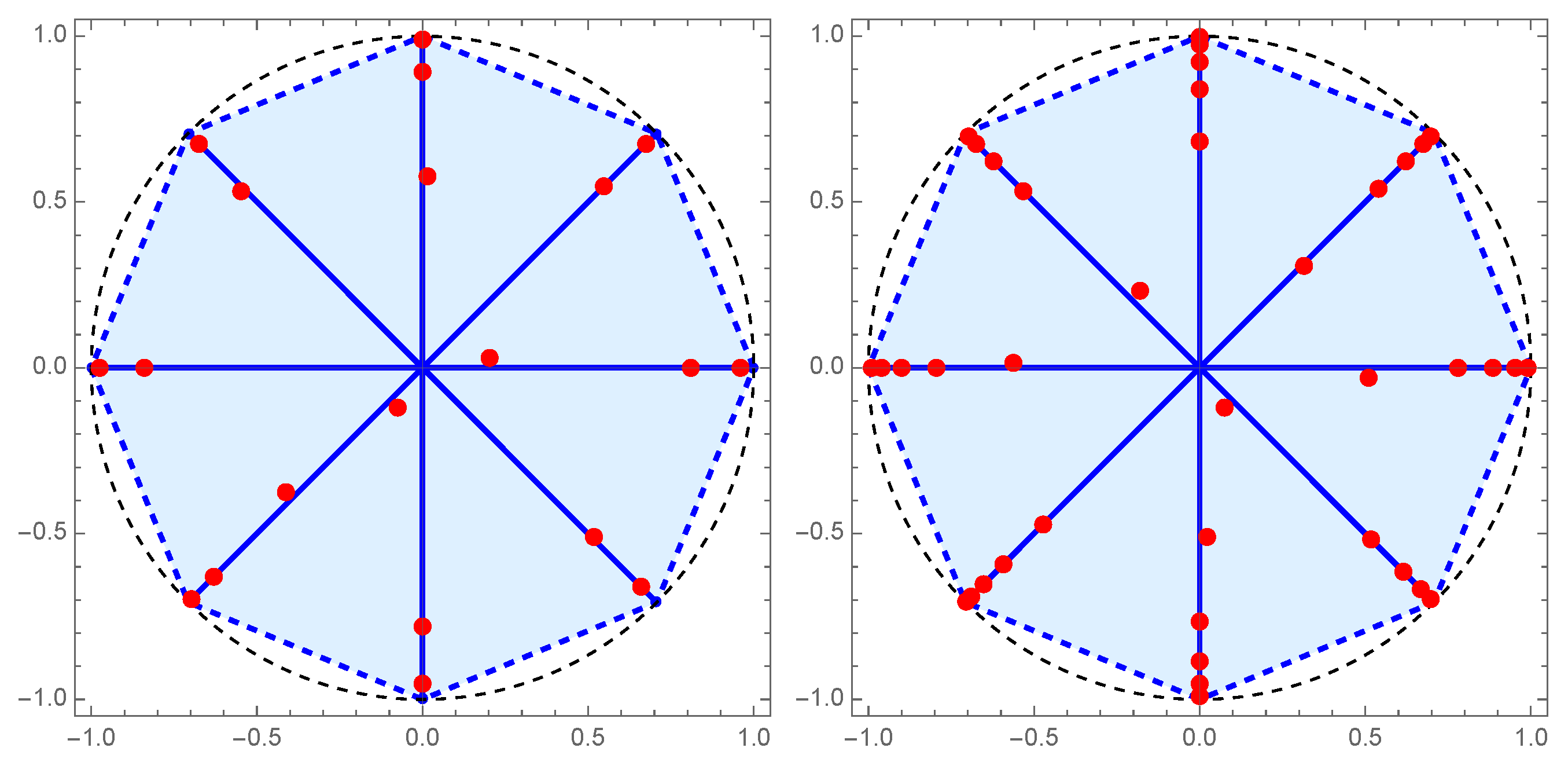
Here we consider eight rays () and the inner product (27), with eight different Jacobi weights on :
Using the discretized Stieltjes-Gautschi procedure, we calculate , so that we are able now to construct all polynomials for and determine their zeros by solving the eigenvalue problem for the Hessenberg matrix .
To save space, now we only mention the matrix , whose elements are given with only a few decimal digits,
The first five orthogonal polynomials are
6. Symmetric Cases of Orthogonal Polynomials on the Radial Rays
In some special cases it is possible to find the moment determinants in an explicit form. Then we can get the corresponding orthogonal polynomials, as well as some other properties of these orthogonal polynomials, including recurrence relations, zero distribution, or even an electrostatic interpretation of their zeros (see [6]).
6.1. Symmetrical Case of Equal Rays, Equidistantly Spaced and with the Same Weight Function
Consider the symmetric case with , , , with the same weight function on the rays
Some of such cases are presented in Examples 1 and 2, with Legendre weight on , except Example 2 (ii)), where we used on .
The inner product, in this case, becomes
and the moments are given by (see also (9))
Note that and . Like in [2] we get that
as well as the following result (see [3]):
Theorem 5.
In the case of even number of rays , the previous result can be simplified (see [2]). Notice that, in that case, for the inner product we have .
Theorem 6.
Because for , the coefficients are arbitrary for , and we can take, e.g., for
Remark 4.
We return again to the general case. For , where and , we see that (31) reduces to
so that, for and , we have
etc. We can conclude that the monic polynomials can be expressed in the following form, with the real coefficients,
where and . Thus, we have the following representation
where , , are monic polynomials of the degree k. Putting (34) in (33), we get
i.e., the following result (see [3]).
Theorem 7.
For each , the monic polynomials satisfy the three-term recurrence relations
with , , where and for , , and . Moreover, these polynomials are orthogonal on with respect to the weight function
where is the weight function in the inner product (29).
6.2. Zero Distribution
The following theorem gives the zero distribution of the polynomials .
Theorem 8.
All zeros of the orthogonal polynomials , , related to the inner product (29), are simple and lie on the radial rays, with possible exception of a multiple zero at the origin of the order ν if .
Let , , denote the zeros of the polynomial , defined in (34), in an increasing order, i.e.,
Then each zero generates M zeros
of the polynomial . On each ray we have
If , where and , then there exists one zero of of order at the origin .
6.3. Legendre Weight on
Let be Jacobi weight on the interval , where . Suppose this weight on all rays, i.e., the inner product (29) in the form
Then, the moments (36) become
i.e.,
and in other cases. In fact, this is a special case of the general one considered earlier in § 5.4. Here, we study Legendre’s case () in particular, for which we can obtain some analytical results.
Thus, we take and the moments (36) become
i.e., for and ,
Lemma 1.
The value of is
Using Theorem 1 and the previous lemma we calculate the norm of the orthogonal polynomial in this symmetric case, when , and , because (see Eq. (13))
Theorem 9.
We have
where .
Using these explicit expressions we can state the following corollary of Theorem 5, for the Legendre weight.
Corollary 1.
Example 7.
Consider now an interesting simple case when (even number of rays ) and inner product is given by (15), as in Example 2 (i). Then, Theorem 6 reduces to following result (see [2]):
Corollary 2.
The sequence of monic orthogonal polynomials , related to the inner product (15), satisfies the recurrence relation
with , , where
6.4. An analogue of the Jacobi polynomials
We consider a symmetric case of M unit rays, equidistantly spaced (, ), with the same weight function on the rays
The inner product given by
Let be the monic Jacobi polynomial on , orthogonal with respect to the weight function . It is connected with the standard monic Jacobi polynomial on as
Using the three-term recurrence relation for (cf. [11], p. 132) we obtain the corresponding recurrence relation for the polynomial ,
where
and
According to Theorems 5 and 7 we can prove the following result:
Theorem 10.
Remark 5.
The case when was considered in [2].
6.5. Some Analogs of the Generalized Laguerre and Hermite Polynomials
We consider now a symmetric case of M infinity rays, equidistantly spaced as in $6.4, with the same weight function on the rays
and the inner product given by
With denote the monic generalized Laguerre polynomials orthogonal related to the weight function on . Such polynomials satisfy the three-term recurrence relation ([11], p. 141)
Using Theorems 5 and 7 we can prove the following result:
Theorem 11.
Remark 6.
The case when was considered in [1,2]. Then, according to Theorem 6, the polynomials , , satisfy (32), where for
Recently, Bouzeffour [8] (see also [9]) used these polynomials to introduce the extended Dunkl oscillator, writing the inner product (41) in the simpler form
with the generalized Hermite weight on .
6.6. Differential equation
In the completely symmetric case, with M rays, using (34), we can prove the following result (cf. [3]).
Theorem 12.
If polynomials , , defined in (34), satisfy linear differential equations of the second order of the form
then the monic orthogonal polynomial satisfies the following second-order linear differential equation
where
Starting from the Jacobi differential equation for (cf. [41], p. 781)
i.e., from the corresponding equation for polynomials orthogonal on ,
and Theorem 12, we conclude that the monic polynomials from Theorem 11 satisfy the second-order linear differential equation
Similar result can be obtained for orthogonal polynomials from Theorem 11 (see [1]).
6.7. Electrostatic Interpretation of the Zeros of Orthogonal Polynomials
As an application of our polynomials , orthogonal on the symmetric radial rays in the complex plane, we give an electrostatic interpretation of their zeros. We mention that the first electrostatic interpretation for the zeros of Jacobi polynomials was given in 1885 by Stieltjes ([42,43]), who studied an electrostatic problem with particles of positive charge p and q placed at the points and , respectively, and with n unit charges placed on the interval at the points , . Assuming a logarithmic potential, Stieltjes showed that the electrostatic equilibrium occurs when , , are zeros of the Jacobi polynomial , where the parameters and take values and , respectively. In that case, the energy of this electrostatic system, defined by Hamiltonian
reaches its minimum. Indeed, this is a unique global minimum of (see Szegő [26], p. 140). There are several results on the similar electrostatic problems (cf. [5,6,26]).
Here we consider a symmetric electrostatic problem with M positive charges of the same strength q, placed at the fixed points , , and a charge of strength p at the point , as well as n positive free unit charges, positioned at the points , , …, . Assuming a logarithmic potential, it is interesting to find the positions of these n points, so that this electrostatic system be in equilibrium.
As in [6] we are interested only in a solution with the rotational symmetry. Denoting , with , , and using the approach of equilibrium conditions from [6], we arrive at the differential equation
Comparing this equation with (42), we find that
as well as , so that the following result holds:
Theorem 13.
The previous electrostatic system is in equilibrium if the points , , are zeros of the polynomial , orthogonal with respect to (38), with . This monic polynomial , where and , can be expressed in terms of the monic Jacobi polynomials as .
7. Concluding Remarks
The main concept on orthogonal polynomials on the radial rays is presented, including existence and uniqueness, a general method for constructing, the main properties and some applications. Special attention is paid to completely symmetric cases.
Funding
This work was supported in part by the Serbian Academy of Sciences and Arts (Φ-96).
Conflicts of Interest
The author declares no conflict of interest.
References
- Milovanović, G.V. Generalized Hermite polynomials on the radial rays in the complex plane, In: Theory of Functions and Applications, Collection of Works Dedicated to the Memory of M.M. Djrbashian (H.B. Nersessian, ed.), pp. 125–29, Yerevan, Louys Publishing House, 1995.
- Milovanović, G.V. A class of orthogonal polynomials on the radial rays in the complex plane, J. Math. Anal. Appl., 206 (1997), 121–139.
- Milovanović, G.V.; Rajković, P.M.; Marjanović, Z.M. A class of orthogonal polynomials on the radial rays in the complex plane, II, Facta Univ. Ser. Math. Inform. 11 (1996), 29–47.
- Milovanović, G.V.; Rajković, P.M.; Marjanović, Z.M. Zero distribution of polynomials orthogonal on the radial rays in the complex plane, Facta Univ. Ser. Math. Inform., 12 (1997), 127–142.
- Milovanović, G.V. Orthogonal polynomials on the radial rays in the complex plane and applications, Rend. Circ. Mat. Palermo (2) Suppl., 68 (2002), 65–94.
- Milovanović, G.V. Orthogonal polynomials on the radial rays and an electrostatic interpretation of zeros, Publ. Inst. Math. (Beograd) (N.S.), 64 (78) (1998), 53–68.
- Deaño, A.; Huybrechs, D.; Iserles, A. Computing Highly Oscillatory Integrals, Society for Industrial and Applied Mathematics (SIAM), Philadelphia, PA, 2018.
- Bouzeffour, F. The extended Dunkl oscillator and the generalized Hermite polynomials on the radial lines, J. Nonlinear Math. Phys. 31:56 (2024), 13 pp.; [CrossRef]
- Bouzeffour, F. Supersymmetric Quesne-Dunkl quantum mechanics on radial lines, Symmetry 2024, 16, 1508. [CrossRef]
- Gautschi, W. Orthogonal Polynomials: Computation and Approximation, Clarendon Press, Oxford, 2004.
- Mastroianni, G.; Milovanović, G.V. Interpolation Processes: Basic Theory and Applications, Springer, Berlin – Heidelberg, 2008.
- Golub, G.; Welsch, J.H. Calculation of Gauss quadrature rules, Math. Comp. 23 (1969), 221–230.
- Agarwal, R.P.; Milovanović, G.V. A characterization of the classical orthogonal polynomials, In: Progress in Approximation Theory (P. Nevai, A. Pinkus, eds.), pp. 1–4, Academic Press, New York, 1991.
- Agarwal, R.P.; Milovanović, G.V. Extremal problems, inequalities, and classical orthogonal polynomials, Appl. Math. Comput. 2001 128, 151–166.
- Al-Salam, W. A. Characterization theorems for orthogonal polynomials, In: Orthogonal Polynomials – Theory and Practice (P. Nevai, ed.), pp. 1–24, NATO ASI Series, Series C; Mathematical and Physical Sciences, Vol. 294, Kluwer, Dordrecht, 1990.
- Gautschi, W. On generating orthogonal polynomials, SIAM J. Sci. Statist. Comput. 3 (1982), 289–317.
- Milovanović, G.V. Construction of s-orthogonal polynomials and Turán quadrature formulae, In: Numerical Methods and Approximation Theory III (Niš, 1987), pp. 311–328, University of Niš, Faculty of Electronic Engineering, Niš, 1988.
- Gautschi, W.; Milovanović, G.V. S-orthogonality and construction of Gauss-Turán type quadrature formulae, J. Comput. Appl. Math. 86 (1997), 205–218. [CrossRef]
- Milovanović, G.V. Quadratures with multiple nodes, power orthogonality, and moment-preserving spline approximation, Numerical analysis 2000, Vol. V, Quadrature and orthogonal polynomials J. Comput. Appl. Math. 127 (2001), no. 1-2, 267–286.
- Milovanović, G.V.; Pranić, M.S.; Spalević, M.M. Quadrature with multiple nodes, power orthogonality, and moment-preserving spline approximation, Part II, Appl. Anal. Discrete Math. 13 (2019), 1–27.
- Milovanović, G.V.; Stanić, M. Construction of multiple orthogonal polynomials by discretized Stieltjes-Gautschi procedure and corresponding Gaussian quadrature, Facta Univ. Ser. Math. Inform. 18 (2003), 9–29.
- Cvetković, A.S.; Milovanović, G.V. The Mathematica Package “OrthogonalPolynomials”, Facta Univ. Ser. Math. Inform. 19 (2004), 17–36.
- Milovanović, G.V.; Cvetković, A.S. Special classes of orthogonal polynomials and corresponding quadratures of Gaussian type, Math. Balkanica 26 (2012), 169–184.
- Szegő, G. Beiträge zur Theorie der Toeplitzschen Formen, Math. Z. 6 (1920), 167–202.
- Szegő, G. Beiträge zur Theorie der Toeplitzschen Formen. II, Math. Z. 9 (1921), 167–190.
- Szegő, G. Orthogonal Polynomials, 4th edns., Amer. Math. Soc. Colloq. Publ. Vol. 23, Amer. Math. Soc., Providence, R.I., 1975.
- Simon, B. Orthogonal Polynomials on the Unit Circle, Part 1. Classical Theory, Amer. Math. Soc. Colloq. Publ., 54, Part 1 American Mathematical Society, Providence, RI, 2005.
- Simon, B. Orthogonal Polynomials on the Unit Circle, Part 2. Spectral Theory, Amer. Math. Soc. Colloq. Publ., 54, Part 2, American Mathematical Society, Providence, RI, 2005.
- Geronimus, Ya.L. Polynomials Orthogonal on a Circle and Interval, Pergamon, Oxford, 1960.
- Gautschi, W.; Milovanović, G. V. Polynomials orthogonal on the semicircle, J. Approx. Theory, 46 (1986), 230–250.
- Gautschi, W.; Landau, H. J.; Milovanović, G. V. Polynomials orthogonal on the semicircle. II, Constr. Approx., 3 (1987), 389–404.
- Calio’, F.; Frontini, M.; Milovanović, G. V. Numerical differentiation of analytic functions using quadratures on the semicircle, Comput. Math. Appl. 22 (1991), 99–106.
- Milovanović, G. V. Some applications of the polynomials orthogonal on the semicircle, In: Numerical Methods (Miskolc, 1986), pp. 625–634, Colloquia Mathematica Societatis Janos Bolyai, Vol. 50, North-Holland, Amsterdam – New York, 1987.
- Milovanović, G. V. Complex orthogonality on the semicircle with respect to Gegenbauer weight: theory and applications, In: Topics in Mathematical Analysis (Th. M. Rassias, ed.), pp. 695–722, Ser. Pure Math., 11, World Sci. Publ., Teaneck, NJ, 1989.
- Milovanović, G. V. Special cases of orthogonal polynomials on the semicircle and applications in numerical analysis, Bull. Cl. Sci. Math. Nat. Sci. Math. 44 (2019), 1–28.
- Milovanović, G. V. Orthogonality on the semicircle: old and new results, Electron. Trans. Numer. Anal. 59 (2023), 99–115. [CrossRef]
- Chihara, T. S. An Introduction to Orthogonal Polynomials, Gordon and Breach, New York, 1978.
- Saff, E. B. Orthogonal polynomials from a complex perspective, In: Orthogonal Polynomials – Theory and Practice (P. Nevai, ed.), NATO ASI Series, Series C; Mathematical and Physical Sciences, Vol. 294, Kluwer, Dordrecht, 1990, pp. 363–393.
- Smith, R., Similarity solutions of a non linear differential equation, IMA J. Appl. Math. 28 (1982), 149–160.
- Smith, R., An abundance of orthogonal polynomials, IMA J. Appl. Math. 28 (1982), 161–167.
- Abramowitz, M.; Stegun, I. A. (Eds), Handbook of Mathematical Functions with Formulas, Graphs, and Mathematical Tables, National Bureau of Standards, Applied Mathematics Series 55, Reprint of the 1972 edition, Dover Publications, Inc., New York, 1992.
- Stieltjes, T. J., Sur quelques théorèmes d’algébre, C.R. Acad. Sci. Paris 100 (1885), 439–440 [Oeuvres Complètes, Vol. 1, pp. 440–441].
- Stieltjes, T. J., Sur les polynômes de Jacobi, C.R. Acad. Sci. Paris 100 (1885), 620–622 [Oeuvres Complètes, Vol. 1, pp. 442–444].
| 1 | Polynomials with complex coefficients. |
Figure 1.
The rays in the complex plane (case with ).
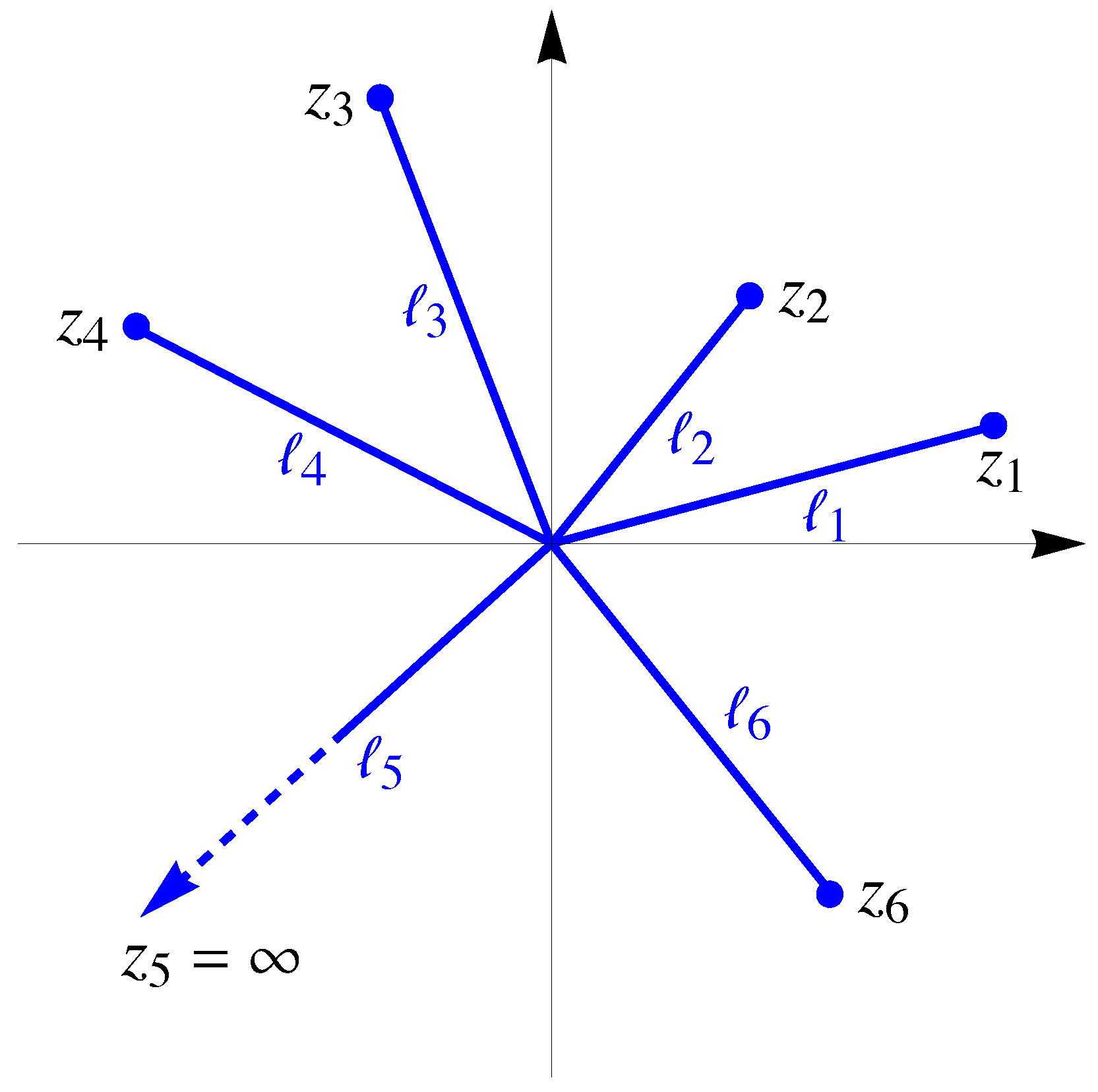
Figure 2.
Three rays , , in the complex plane, given by the complex points , .
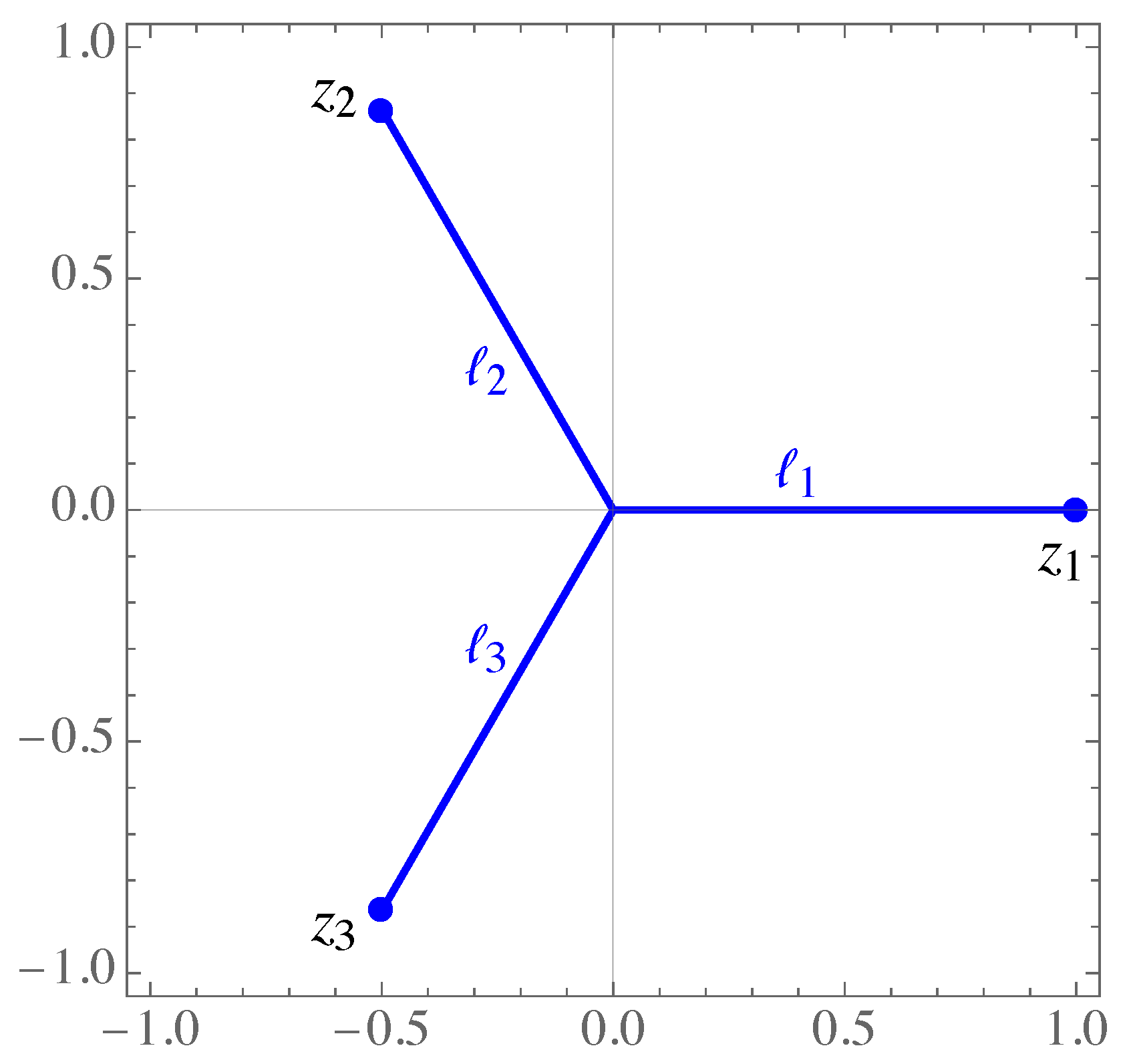
Figure 3.
Zeros of (), with the Legendre weight , lie in the convex hull of the rays (left) and on the concentric circles (right).
Figure 3.
Zeros of (), with the Legendre weight , lie in the convex hull of the rays (left) and on the concentric circles (right).
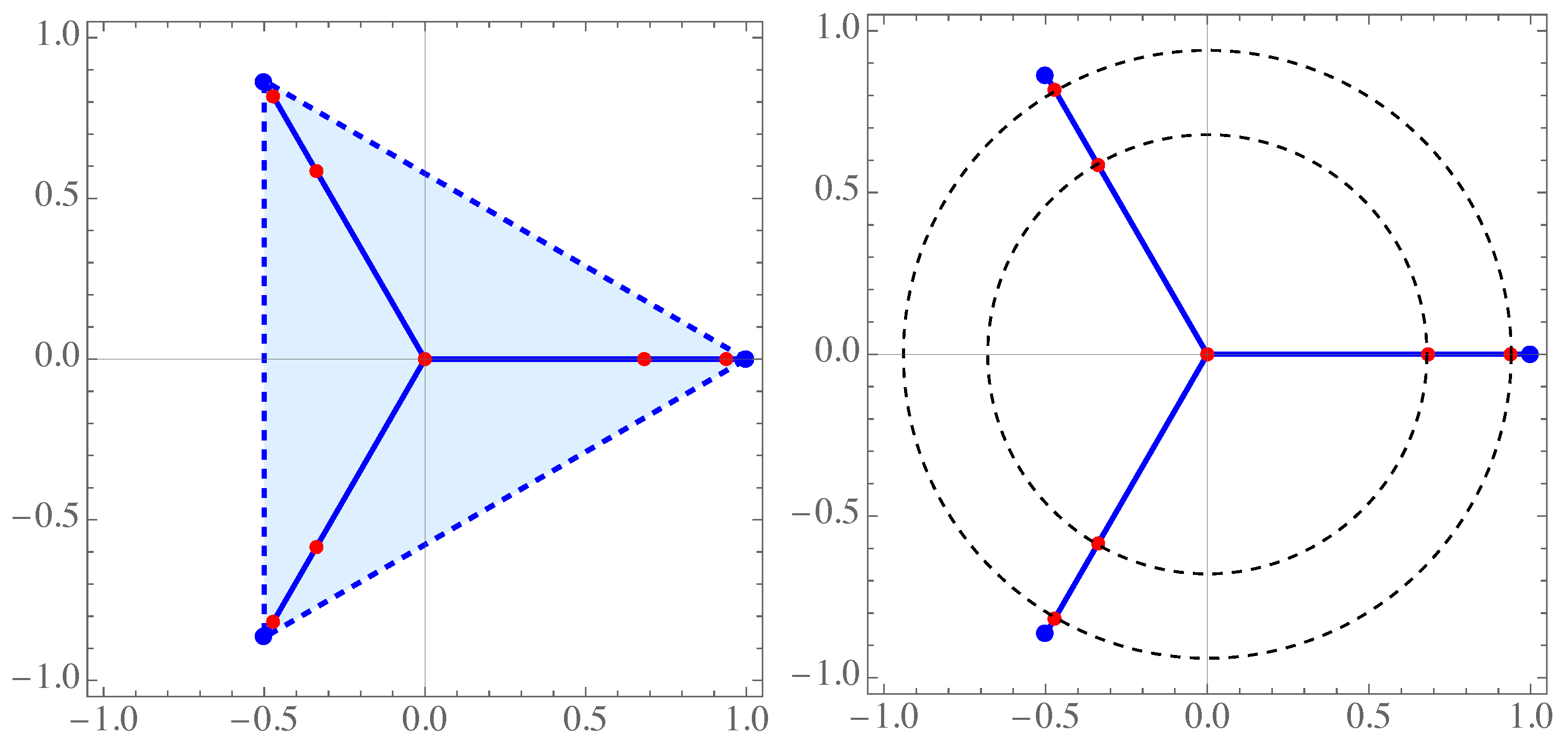
Figure 4.
Zeros of the orthogonal polynomials for in Example 3.
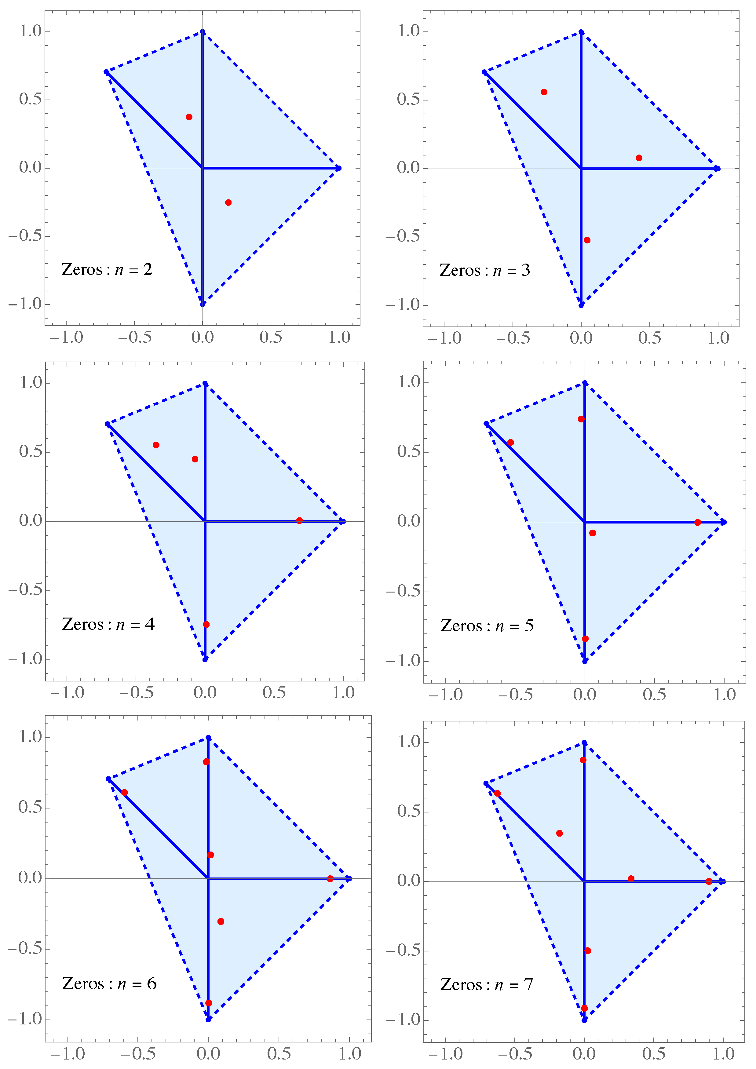
Figure 5.
Zeros of the orthogonal polynomials (brown), (red) and (grren) in Example 4.
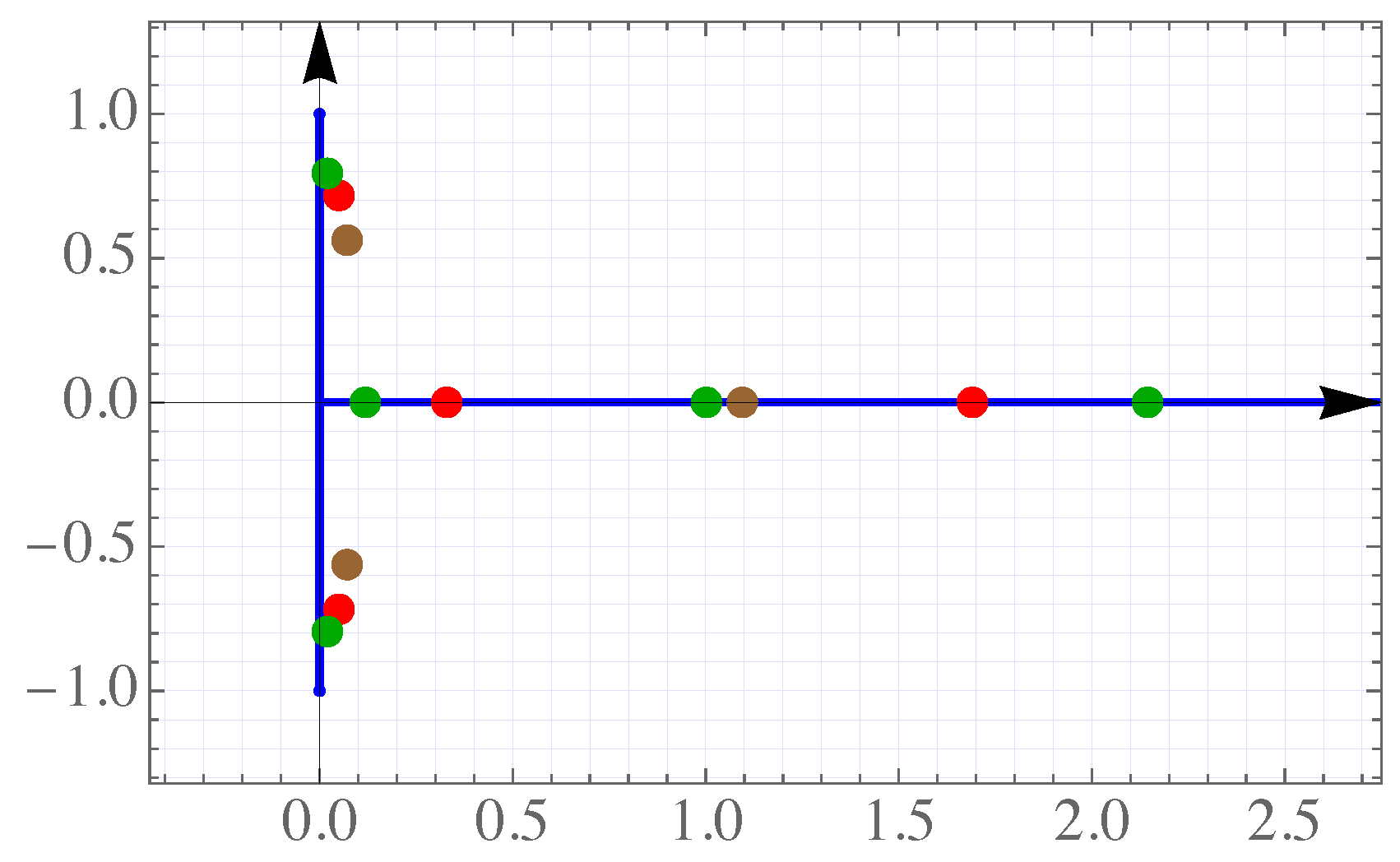
Figure 6.
Zeros of polynomials of degree (left) and (right) for Chebyshev weight of the first kind on rays.
Figure 6.
Zeros of polynomials of degree (left) and (right) for Chebyshev weight of the first kind on rays.
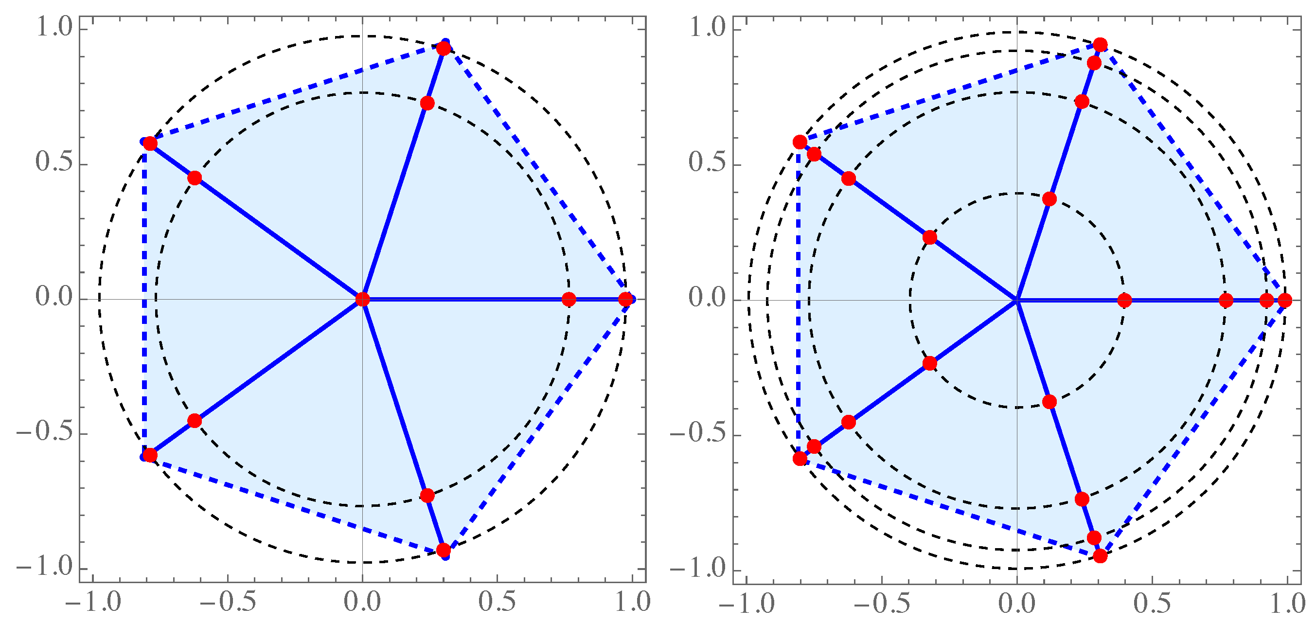
Figure 7.
Zeros of polynomials of degree (left) and (right) for Chebyshev weight of the second kind on rays.
Figure 7.
Zeros of polynomials of degree (left) and (right) for Chebyshev weight of the second kind on rays.
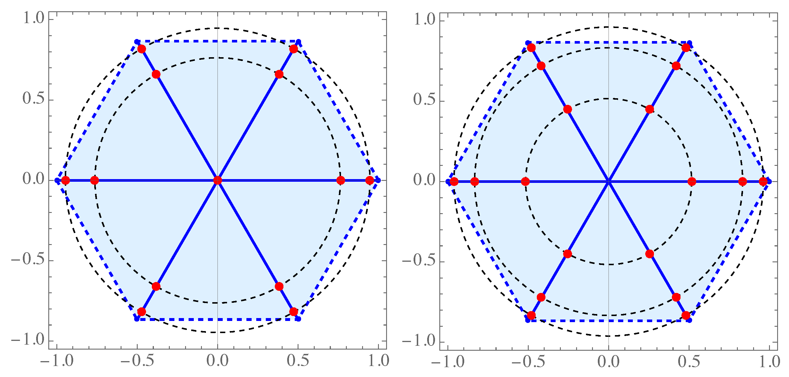
Figure 8.
Zeros of (left) and (right) in Example 6.
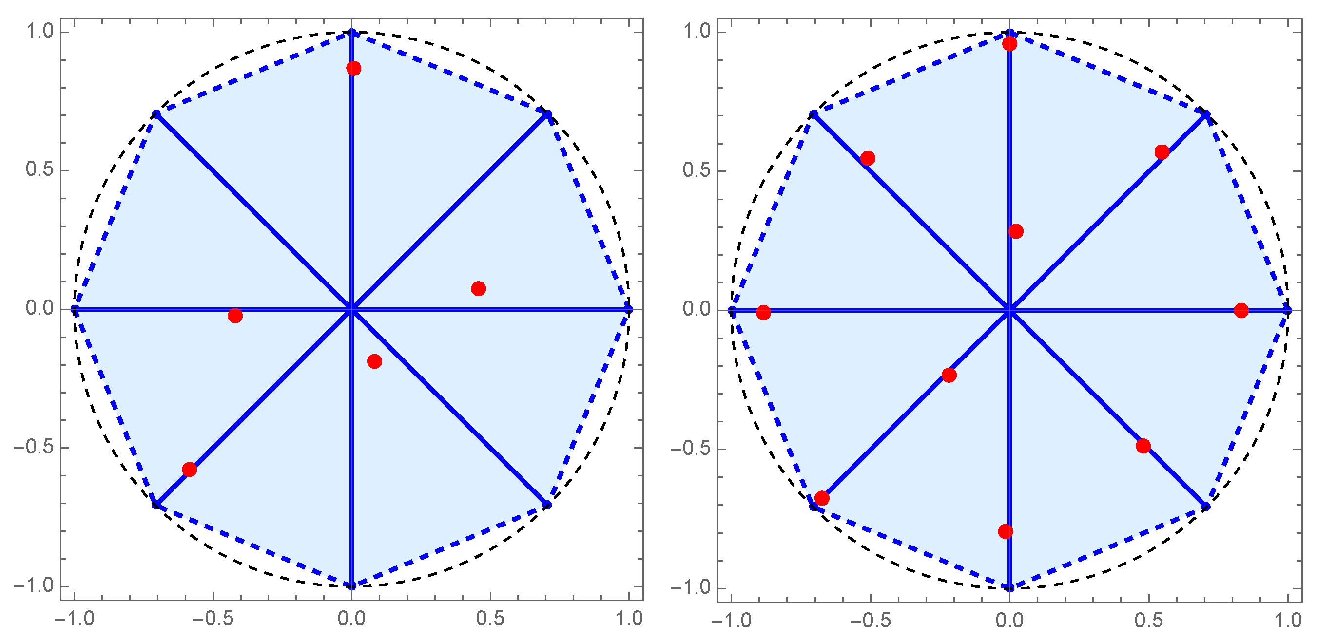
Figure 9.
Zeros of (left) and (right) in Example 6.
Disclaimer/Publisher’s Note: The statements, opinions and data contained in all publications are solely those of the individual author(s) and contributor(s) and not of MDPI and/or the editor(s). MDPI and/or the editor(s) disclaim responsibility for any injury to people or property resulting from any ideas, methods, instructions or products referred to in the content. |
© 2024 by the author. Licensee MDPI, Basel, Switzerland. This article is an open access article distributed under the terms and conditions of the Creative Commons Attribution (CC BY) license (https://creativecommons.org/licenses/by/4.0/).
Copyright: This open access article is published under a Creative Commons CC BY 4.0 license, which permit the free download, distribution, and reuse, provided that the author and preprint are cited in any reuse.