Multiple Time-Scale Pattern Classification Using a Refinement Fuzzy Min-Max Neural Network

1. Introduction

Pattern classification is concerned with categorizing given samples into certain classes by obtaining and analyzing the features of samples [1]. Due to its ability to find categorical labels for a set of observations, it has been an active area and widely used in a number of real-world applications, including weather forecasting, defense, medicine, industry, behavior analysis, and speech recognition [2]. While many mathematical methods have concentrated on realizing pattern classification, their ability to learn knowledge from data as well as self-adaption is less promising [3]. Resorting for more powerful tools, many machine learning models have appeared as effective classifiers [4]. They can absorb knowledge from collected samples and subsequently use the features of new samples to make inferences about the corresponding classes [5].

In pattern classification, machine learning models that are commonly used as effective classifiers including artificial neural networks (ANNs) [6], support vector machine (SVM) [7], Naive Bayes [8], k-nearest neighbor [9], decision tree [10], and random forest [11]. Among them, ANNs can approximate any unknown nonlinear systems and are equipped with self-learning abilities. In the currently popular techniques related to ANNs, the fuzzy neural network (FNN) is a composite method that combines the essential idea of the fuzzy theory into the framework of ANN. Due to FNN making full use of the advantages of ANN and fuzzy theory, it possesses the capabilities of self-learning, self-adaptability, and self-organization. This merit made it very popular in the machine learning community and has been widely used as a strong classifier in real-world applications concerning pattern recognition [12].

There has been plenty of work focused on the design and improvement of FNN. To name a few, Simpson et al. proposed a supervised learning neural network classifier named fuzzy min-max (FMM) neural network. It features utilizing fuzzy sets with min-max boundaries for reliable pattern classification [13]. Identically, an unsupervised fuzzy min-max clustering neural network was also proposed, in which clusters are implemented as fuzzy sets using a membership function with a hyper box [14]. The hyperbox locates the fuzzy region of the corresponding class in the feature space. Despite these efforts, they may be limited to certain problems. For improvement, Gabrys et al. [15] proposed a general FMM model called a general fuzzy min-max neural network (GFMM). GFMM improves the original model and adapts it to a new type of data. These modifications include the formulation of the expansion equation, the design of the membership function, as well as the structure of the network. The above-mentioned methods commonly utilize the origin features as input instead of taking feature importance into account. To handle this issue, Liu et al. [16] developed an adaptive fuzzy (AFMN) classifier based on the principal component analysis (PCA) and adaptive genetic algorithm (GA) to improve the classification performance of FMM. There are still several limitations in the original FMM network, such as the redundant hyperboxes and overlap regions. Mohammed et al. presented an enhanced fuzzy min-max (EFMM) model to overcome these limitations [17]. There are three heuristic adjustment rules for improving the training phase of FMM in EFMM, which are the modified expansion, overlap test, and contraction procedures, respectively. Although significant improvements on the original FMM model have been proposed above, FMM variants with contraction suffer from the problem of data distortion [18].

To solve the problem, another category of FMM modifications focuses on eliminating the contraction procedure from the learning stage [19]. For example, Nandedkar et al. [20] proposed a supervised classification model with compensatory neurons (CNs), called the fuzzy min-max neural network classifier with compensatory neurons (FMCN). Based on the CN architecture, FMCN supports online learning that can effectively alleviate the influence of data distortion. Zhang et al. proposed a data core FMM (DCFMN) model for pattern classification [21]. DCFMN updates the FMM structure using classifying and overlapping neurons. Furthermore, a new membership function for classifying and overlapping neurons is designed, which takes into account noise, geometric center, and data core to suppress data distortion and ensure accurate classification. Moreover, Davtalab et al. proposed an MLF using two types of subnets to improve classification accuracy in the overlap regions [22]. Each node in MLF is known as a subnet and acts as an independent classifier. The above methods used more neurons to overcome data distortion and then improve the performance of the FMM classifier. However, the above method cannot deal with multiple time-scale information that is common in practice [23]. This drawback may result in their failure to make useful predictions about true labels of samples with the time-scale of features varying.

To solve the above problem, in this paper, a refinement of fuzzy production rules by using a fuzzy min-max neural network (FPR-FMM) is proposed. FPR-FMM can use the idea of fuzzy production to deal with samples with multiple times-scale features, which facilitates multiple time-scale pattern classification. The main contributions are as follows:

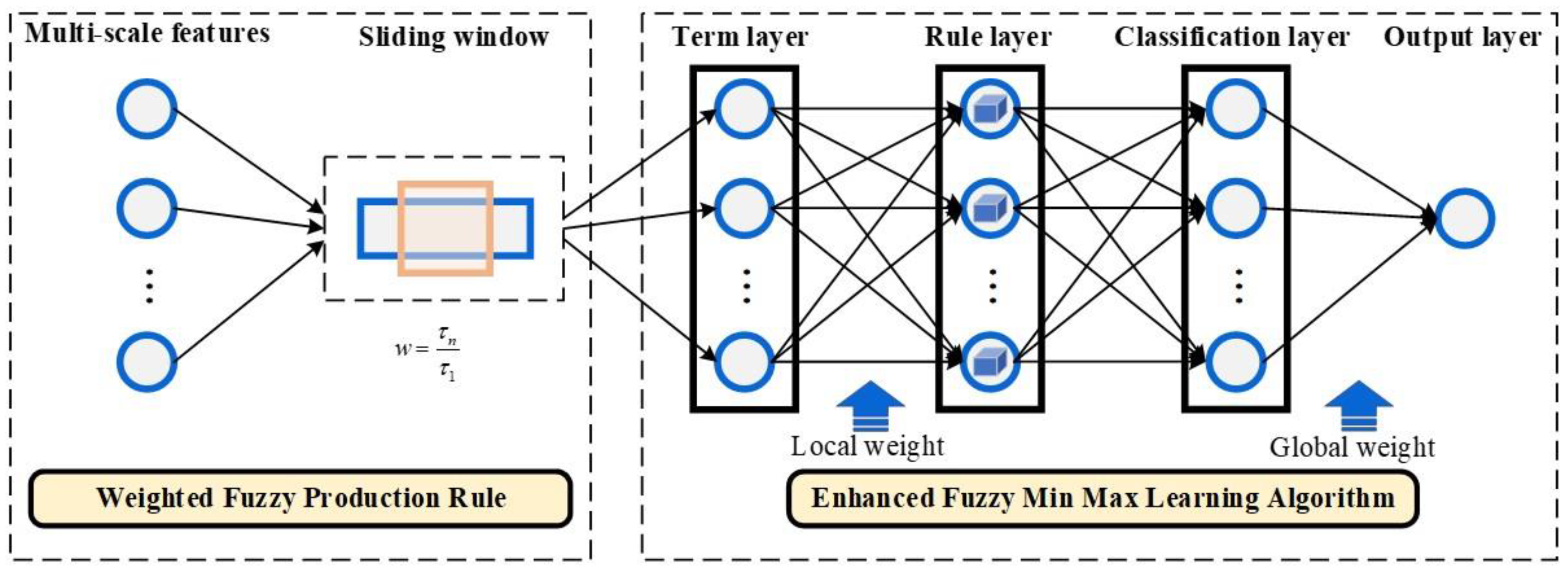
• A new classification (membership) function is established based on multiple time-scale characteristics, where local and global weights are established based on the multiple time-scale input pattern. Then it can directly utilize origin features for pattern classification.
• An improved fuzzy min-max learning algorithm is proposed. The approximation of the FMM is utilized to improve the refinement of the local and global parameters in FPR, which ensures accurate classification.
• A pruning strategy is designed. This strategy concentrates on removing redundant fuzzy rules represented by hyperboxes, thereby enhancing the classification ability of FPR-FMM while eliminating the influences of redundant information.

The remainder of the paper is organized as follows. Section 2 discusses the background and the problem description. In Section 3, an FPR-FMM model based on new rules is designed, which is followed by an enhanced learning algorithm that is discussed in Section 4. Section 5 shows the experimental results and discussions after implementation. Finally, the conclusion is given in Section 6.

2. Problem Description

Defining the time scale vector τ in the case of multiple time-scale sampling systems, which is described as:

$$\mathit{\tau }=\left[{\tau }_1,{\tau }_2,\mathrm{...},{\tau }_n\right],$$

(1)

where τ_i is a positive integer, i=1, 2, …, n, n≥1 are natural numbers and τ₁ ≤ τ₂ ≤ … ≤ τ_n. The corresponding sampling time of each sampling scale is described as:

$$\left\{\begin{array}{l}{t}_1=t_0+k{\tau }_1\\ t_2=t_0+k{\tau }_2\\ \mathrm{......}\\ t_n=t_0+k{\tau }_n\end{array}\right.,$$

(2)

where t₀ is the initial sampling time, t_i is the sampling time corresponding to the ith time scale τ_i, k=0, 1, …, K_n, and K_n≥0 is a natural number.

According to the multi-scale analysis, the sampling matrix is defined as:

$$X=\left[{\mathbf{x}}_1\left(t_1\right),{\mathbf{x}}_2\left(t_2\right),\dots ,{\mathbf{x}}_n\left(t_n\right)\right],$$

(3)

where x_i(t_i) is the sampled data vector at time t_i.

Because there may be multiple relationships between the sampling time scales, the sampling time of different scale features may overlap. According to Eq.(2), the index set I corresponding to the time scale of the feature obtained at the current time is given as:

$$\mathit{I}=\left\{i:\mathrm{if}t=t_0+k{\tau }_i\right\},$$

(4)

where t is the current time. Combined with formula (3), all the features X_f(t) that can be obtained at time t are expressed as:

$${\mathbf{X}}_f(t)=\left[x_{I[1]}(t),x_{I[2]}(t),\mathrm{...},x_{I[l]}(t)\right],$$

(5)

where l = ||I||, I[s] denotes the sth element in I.

It can be seen from the above that the features that can be obtained at different times t are variable. However, the traditional fuzzy min-max neural network cannot deal with multiple time-scale variables.

3. FPR-FMM

In this section, detailed descriptions of the proposed FPR-FMM are given, and the related illustration is presented in Figure 1. In the following, we will introduce the weighted fuzzy production rule and the architecture of FPR-FMM, respectively.

3.1. Weighted Fuzzy Production Rule (WFPR)

To solve the above problem, a sliding window is set to extract the change range of each time scale feature. By designing fuzzy rules, the multi-scale features are preprocessed.

The size of the sliding window is formulated as:

$$w={\displaystyle \frac{{\tau }_n}{{\tau }_1}},$$

(6)

the sliding window is placed at the starting point of the sampled data vector x_i(t_i), forming a data segment with a data length of w. The initial time is set to t, and extracting the value range [x_i^l(t), x_i^u(t)] of the i-th scale variable in the window.

Consider a set of fuzzy production rules S = {R_i, i = 1, 2, …, m}, where R_i is expressed as:

$$\begin{array}{l}{R}_i:\mathrm{If}\left(x_1^l(t)\mathrm{is}{A}_{1i}^l(t)\left[v_{1i}(t)\right]and{x}_1^u(t)\mathrm{is}{A}_{1i}^u(t)\left[w_{1i}(t)\right]\right)\hfill \\ \mathrm{AND}\mathrm{......}AND\left(x_n^l(t)\mathrm{is}{A}_{ni}^l(t)\left[v_{ni}(t)\right]and{x}_n^u(t)\mathrm{is}{A}_{ni}^u(t)\left[w_{ni}(t)\right]\right)\hfill \\ \mathrm{THEN}C\mathrm{is}{C}_i\left[U_i(t)\right],\end{array},$$

(7)

where x^l(t)=[x₁^l(t), x₂^l(t), …, x_n^l(t)] and x^u(t)=[x₁^u(t), x₂^u(t), …, x_n^u(t)] respectively represent the upper and lower limit vectors of attributes at time t, C is also the attributes. A_1i^l(t), A_1i^u(t), …, A_ni^l(t), A_ni^u(t) and C_i are the values of these attributes, which are fuzzy. v_ji(t) and w_ji(t) are the local weight of the proposition “x_j^l(t) is A_ji^l(t)” and “x_j^u(t) is A_ji^u(t)” respectively, j=1, 2, …, n, U_i denotes the global weight assigned to the entire rule.

For each rule R_i within S, the similarity between the proposition and the observed attribute-value denoted by SM_ji(t), is defined as the membership value that indicates to what degree the example belongs to the corresponding term. The overall similarity SM_i(t) is defined as:

$$S{M}_i(t)={\min }_{1\le j\le n}S{M}_{ji}(t),$$

(8)

where

$$\begin{array}{l}S{M}_{ji}(t)=\min \left(\left[1-f\left(x_i^u\left(t\right)-w_{ji}\left(t\right),{\gamma }_i\right)\right]\right.,\\ \left.\left[1-f\left(v_{ji}\left(t\right)-x_i^l\left(t\right),{\gamma }_i\right)\right]\right),\end{array}$$

(9)

$$f(x,{\gamma }_i)=\left\{\begin{array}{ll}1,\hfill & \mathrm{if}x{\gamma }_i>1\hfill \\ x{\gamma }_i,\hfill & \mathrm{if}0⩽x{\gamma }_i⩽1\hfill \\ 0,\hfill & \mathrm{if}x{\gamma }_i<0\hfill \end{array}\right.,$$

(10)

where γ=[γ₁, γ₂, …, γ_n] is a sensitive parameter. Accordingly, the hyperbox fuzzy set is defined as:

$$B_i(t)=\{v_i(t),w_i(t),S{M}_i(t)\}.$$

(11)

Let there be k fuzzy sets of conclusions. The conclusions of the given m rules (hyperboxes) can be classified into k groups, denoted by CLASS₁, …, CLASS_k. The inferred result is represented as a vector {c₁(t), c₂(t), …, c_k(t)}. The degree c_k(t) is determined by the following equation:

$$c_k\left(t\right)=\underset{i=1}{\overset{m}{\max }}S{M}_i\left(t\right)U_{ik}(t),$$

(12)

$$U_{ik}(t)=\left\{\begin{array}{l}1,C_i\in CLAS{S}_k\\ 0,otherwise\end{array}\right.,$$

(13)

where c_k(t) is the value that indicates to what degree the input pattern belongs to CLASS_k. When the crisp inferred result is needed, one can take the consequent CLASS_k with maximum c_k(t).

3.2. FPR-FMM architecture

A set of WFPRs and the proposed weighted fuzzy reasoning algorithm can be exactly mapped into a fuzzy min-max (FMM) neural network. The network has a three-layer network structure, including the Term layer, Rule layer, and Classification layer. We describe the structure of the mapped FMM as follows.

Term layer: This is the input layer (layer i). Each node in this layer represents a linguistic term of an attribute. Since each linguistic term corresponds to an attribute value, the input of each node is regarded as the similarity degree between the observed attribute value and the corresponding term (proposition) of the antecedent in a WFPR. The similarity degree can also be the membership value that indicates to what degree the observed fact belongs to the linguistic term.

Rule layer: This is the only hidden layer (layer j), which represents a hyperbox fuzzy set. Each node in this layer represents a given antecedent part of a rule. According to linguistic terms (propositions) that appeared in the antecedent part of a rule, the connections between the term layer and the rule layer are determined.

Classification layer: This is the output layer (layer k). Each node in this layer represents a fuzzy cluster. Since the inferred result of a WFPR is generally the form of a vector (discrete fuzzy set defined on the space of cluster labels), the output of the network has more than one value. The meaning of each output value is the membership value that indicates to what degree the input pattern belongs to the cluster corresponding to the node.

Connection weights: The local weights (shown as v_ij(t) and w_ij(t)) of a set of WFPRs are regarded as the connection weights between the term layer and the rule layer. The global weights (shown as U_ik(t)) of the set of WFPRs are regarded as the connection weights between the rule layer and the classification layer

4. An Enhanced Fuzzy Min Max Learning Algorithm

The architecture of FPR-FMM has been given in Section III. It can process multi-scale features effectively. For this, FMM is first trained using an enhanced learning algorithm and then pruned to reduce the number of hyperboxes created. The learning and pruning algorithm of FPR-FMM are given in this section.

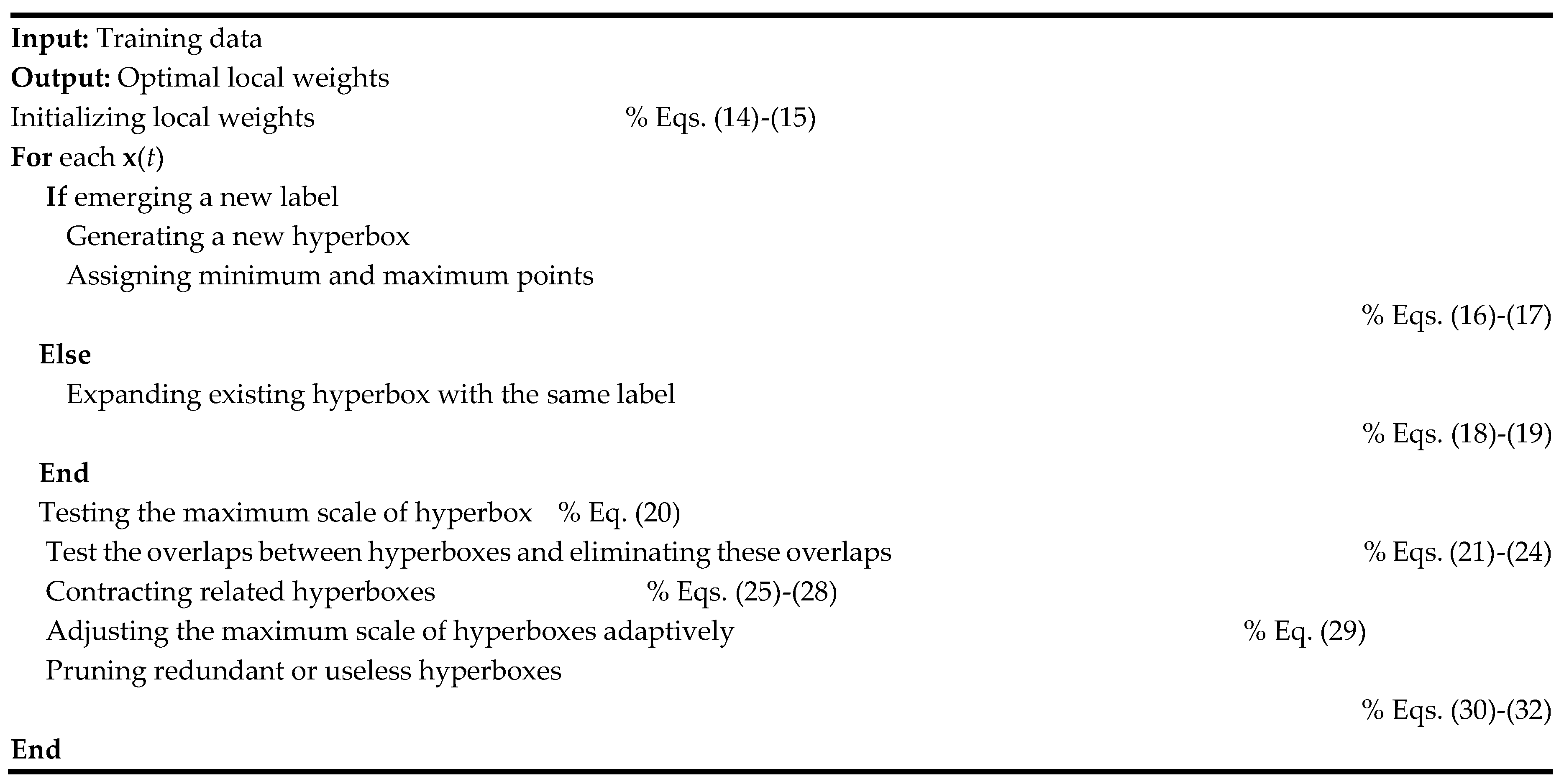
4.1. Learning Algorithm

The learning algorithm consists of four steps: initialization, hyperbox expansion, overlap test, and contraction. The last three steps are repeated according to each input feature vector in the training sample.

• Initialization: The minimum point v_j and maximum point w_j of the jth hyperbox are initialized as follows:

$${\mathbf{v}}_j\left(t\right)=[\underset{N}{\underbrace{1,1,\mathrm{...},1}}],$$

(14)

It can be seen from the above formula that when the jth hyperbox is created for the first time in the expansion process, the minimum and maximum points of the hyperbox can be automatically adjusted as follows according to Eqs. (16) and (17):

$${\mathbf{v}}_j\left(t+1\right)={\mathbf{x}}^l\left(t\right),$$

(16)

$${\mathbf{w}}_j\left(t+1\right)={\mathbf{x}}^u\left(t\right).$$

(17)

2.

Hyperbox expansion: The expansion process is used to determine the number of hyperboxes and their minimum and maximum points. According to the input mode x(t) at time t, the membership degree is calculated, and the hyperbox B_j(t) with the largest membership degree is selected for expansion. In this case, adjust B_j(t) according to Eqs. (18) and (19).

$$v_{ji}\left(t+1\right)=\min \left(v_{ji}\left(t\right),x_i^l\left(t\right)\right),\forall i=1,\dots ,N,$$

(18)

$$$$

(19)

Before expansion, the check of the following expansion conditions is needed:

(a) Hyperbox maximum scale test:

$$\left(\max \left(w_{ji}\left(t\right),x_i^u\left(t\right)\right)-\min \left(v_{ji}\left(t\right),x_i^l\left(t\right)\right)\right)\le \Theta ,\forall i=1,2,\mathrm{...},N,$$

(20)

where Θ is the maximum scale of the hyperbox, which needs to be artificially defined, 0≤Θ≤1.

(b) Class compatibility test: It is necessary to check whether the label of the hyperbox is compatible with the output label when the hyperbox is expanded. Let d(t)∈ {0, 1, 2, …, p} be the output class at time t, p is the number of classes.

i. When d(t) = 0, directly adjust B_j(t) according to (18) and (19);

ii. When d(t) ≠ 0, it is necessary to determine whether or not to adjust according to the label of the hyperbox B_j(t). If the label of the hyperbox B_j(t) is 0, the corresponding category of B_j(t) is assigned as d(t) while adjusting; if the label of the hyperbox B_j(t) is d(t), then directly adjust B_j(t); otherwise, there is no need to adjust the hyperbox B_j(t).

If the above conditions are met, adjust B_j(t) according to Eqs. (18) and (19). If none of the existing hyperboxes contain or cannot be expanded to contain x(t), a new hyperbox B_k(t+1) needs to be initialized according to Eqs. (14) and (15), and then Eqs. (16) and (17) Adjust and set the label of the hyperbox B_k(t+1) to d(t).

3.

Overlap test: FPR-FMM stipulates that overlap between hyperboxes of the same type is allowed, while the overlap between hyperboxes of different types is not allowed. Assuming that the hyperbox B_j(t) is expanded in the previous step, there are two cases to select other hyperboxes that need to be tested for overlap with B_j(t). Suppose any hyperbox B_k(t) and B_j(t) are tested for overlap, then:

(a) If the hyperbox B_j(t) has no label, that is, class(B_j(t))=0, then B_j(t) needs to be tested for overlap with all other hyperboxes.

(b) If the hyperbox B_j(t) has a label, that is, class(B_j(t))≠0, then B_j(t) only needs to be combined with other hyperbox (class(B_j(t))≠class(B_k(t))) for overlap test.

To determine whether the hyperbox B_j(t) has overlapped between different classes after expansion, it is necessary to analyze the above-mentioned hyperboxes B_k(t) and B_j(t) that meet the test conditions dimension by dimension according to the following four situations. As long as any one of them is satisfied, there exists overlap. According to the principle of minimum adjustment [33], only the minimum overlap item of each dimension and the index of the corresponding dimension are saved. The following four scenarios will be considered:

$$\begin{array}{c}case1:v_{ji}\left(t+1\right)<v_{ki}\left(t\right)<w_{ji}\left(t+1\right)<w_{ki}\left(t\right)\\ {\delta }^{\mathrm{new}}=\min \left(w_{ji}\left(t+1\right)-v_{ki}\left(t\right),{\delta }^{\mathrm{old}}\right),\end{array}$$

(21)

$$\begin{array}{c}case2:v_{ki}\left(t\right)<v_{ji}\left(t+1\right)<w_{ki}\left(t\right)<w_{ji}\left(t+1\right)\\ {\delta }^{\mathrm{new}}=\min \left(w_{ki}\left(t\right)-v_{ji}\left(t+1\right),{\delta }^{\mathrm{old}}\right),\end{array}$$

(22)

$$\begin{array}{c}case3:v_{ji}\left(t+1\right)<v_{ki}\left(t\right)\le w_{ki}\left(t\right)<w_{ji}\left(t+1\right)\\ {\delta }^{\mathrm{new}}=\min \left(\min \left(w_{ji}\left(t+1\right)-v_{ki}\left(t\right),\right.\right.\\ \left.w_{ki}\left(t\right)-v_{ji}\left(t+1\right),{\delta }^{\mathrm{old}}\right),\end{array}$$

(23)

$$\begin{array}{c}case4:v_{ki}\left(t\right)<v_{ji}\left(t+1\right)\le w_{ji}\left(t+1\right)<w_{ki}\left(t\right)\\ {\delta }^{\mathrm{new}}=\min \left(\min \left(w_{ji}\left(t+1\right)-v_{ki}\left(t\right),\right.\right.\\ \left.w_{ki}\left(t\right)-v_{ji}\left(t+1\right),{\delta }^{\mathrm{old}}\right),\end{array}$$

(24)

and initially set δ^old=1, ∆=0. If the ith dimension satisfies one of the above four conditions and δ^old-δ^new>0, then δ^old=δ^new, ∆=i, and the record corresponds to the overlapping situation L(L=1, 2, 3, 4); If the above four conditions are not met, ∆=-1, indicating that there is no overlap between B_k(t) and B_j(t) between the hyperboxes, and no contraction is required.

4.

Hyperbox contraction: If there is overlap between different types of hyperboxes, the contracting process will reduce the overlap. When ∆>0, only need to adjust the ∆th dimension between the two hyperboxes. The hyperbox contracts as follows:

$$\begin{array}{c}case1:v_{j\Delta }\left(t+1\right)<v_{k\Delta }\left(t\right)<w_{j\Delta }\left(t+1\right)<w_{k\Delta }\left(t\right)\\ v_{k\Delta }^{\mathrm{new}}\left(t\right)=w_{j\Delta }^{\mathrm{new}}\left(t+1\right)={\displaystyle \frac{v_{k\Delta }^{\mathrm{old}}\left(t\right)+w_{j\Delta }^{\mathrm{old}}\left(t+1\right)}{2}},\end{array}$$

(25)

$$\begin{array}{c}case2:v_{k\Delta }\left(t\right)<v_{j\Delta }\left(t+1\right)<w_{k\Delta }\left(t\right)<w_{j\Delta }\left(t+1\right)\\ v_{j\Delta }^{\mathrm{new}}\left(t+1\right)=w_{k\Delta }^{\mathrm{new}}\left(t\right)={\displaystyle \frac{v_{j\Delta }^{\mathrm{old}}\left(t+1\right)+w_{k\Delta }^{\mathrm{old}}\left(t\right)}{2}},\end{array}$$

(26)

$$\begin{array}{l}case3:v_{j\Delta }\left(t+1\right)<v_{k\Delta }\left(t\right)\le w_{k\Delta }\left(t\right)<w_{j\Delta }\left(t+1\right)\\ \left\{\begin{array}{l}{v}_{j\Delta }^{\mathrm{new}}\left(t+1\right)=w_{k\Delta }^{\mathrm{old}}\left(t\right),w_{k\Delta }\left(t\right)-v_{j\Delta }\left(t+1\right)<w_{j\Delta }\left(t+1\right)-v_{k\Delta }\left(t\right)\\ w_{j\Delta }^{\mathrm{new}}\left(t+1\right)=v_{k\Delta }^{\mathrm{old}}\left(t\right),otherwise\end{array}\right.,\end{array}$$

(27)

$$\begin{array}{l}case4:v_{k\Delta }\left(t\right)<v_{j\Delta }\left(t+1\right)\le w_{j\Delta }\left(t+1\right)<w_{k\Delta }\left(t\right)\\ \left\{\begin{array}{l}{w}_{k\Delta }^{\mathrm{new}}\left(t\right)=v_{j\Delta }^{\mathrm{old}}\left(t+1\right),w_{k\Delta }\left(t\right)-v_{j\Delta }\left(t+1\right)<w_{j\Delta }\left(t+1\right)-v_{k\Delta }\left(t\right)\\ v_{k\Delta }^{\mathrm{new}}\left(t\right)=w_{j\Delta }^{\mathrm{old}}\left(t+1\right),otherwise\end{array}\right..\end{array}$$

(28)

5.

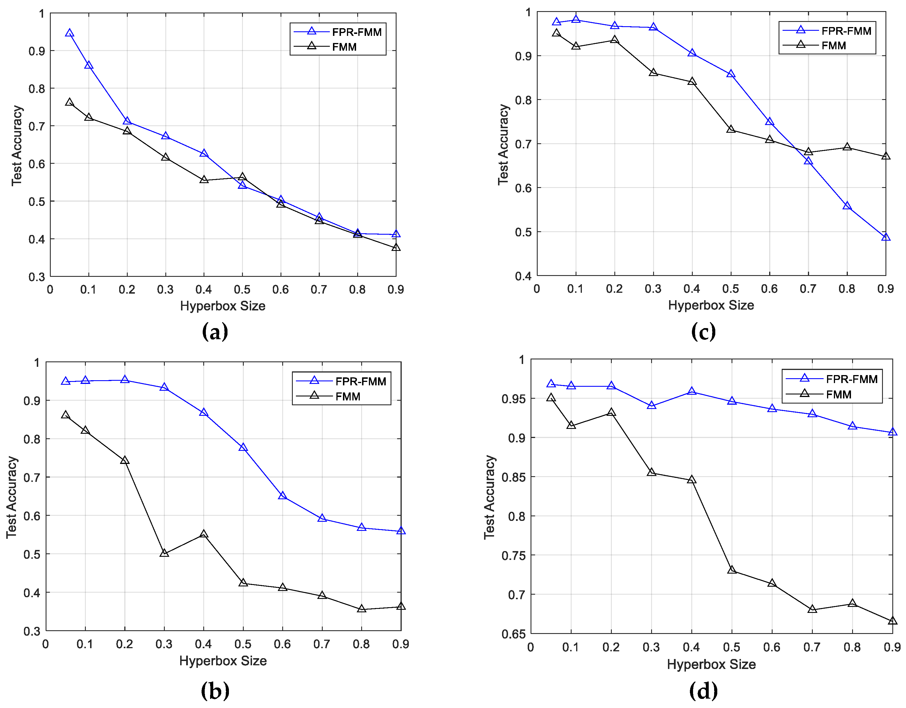
Adaptive adjustment of maximum scale: For hyperbox, the maximum scale Θ has an important influence on the classification of the network. The fixed parameters may lead to a reduction in classification accuracy. When the parameter Θ is large, the number of error classifications will increase, especially when there are complex overlapping classes; on the contrary, when the parameter Θ is small, it will cause a lot of unnecessary expansion of the hyperbox. Therefore, the parameter Θ needs to be dynamically adjusted to improve the classification accuracy of the model. To dynamically adjust the parameters, after each training data is input, the dynamic adjustment formula of parameter Θ is as follows:

$$\Theta (t+1)=\phi \Theta (t),$$

(29)

where φ is the decreasing speed of the hyperbox dimension Θ, 0<φ<1.

4.1. Pruning of hyperboxes based on confidence factor

An effective pruning algorithm is a crucial component of any neural network in the course of learning. In the proposed classification model, the trained network has been pruned to remove the useless hyperboxes based on their confidence factor. The confidence factor identifies the hyperboxes that are frequently used and generally accurate, as well as those that are rarely used but extremely accurate. Based on the usage frequency and accuracy on a training set, the confidence factor of each hyperbox node is defined as:

$$C{F}_j=(1-\alpha )U_j+\alpha A_j,$$

(30)

where U_j∈[0, 1] is the usage of jth hyperbox, A_j∈[0, 1] is its accuracy, and α∈[0, 1] is a weighting factor. The value of U_j is given by

$$U_j=C_j/C_f,$$

(31)

where C_j is the number of patterns classified by hyperbox j for class c_k, and C_f is the number of patterns classified by any hyperbox f for class c_k. The value of A_j is given by

$$A_j=P_j/P_f,$$

(32)

where P_j is the number of patterns correctly classified by hyperbox j for class k, and P_f is the number of patterns correctly classified by any hyperbox f for class k. The hyperboxes with a confidence factor less than or equal to some user-defined threshold are pruned.

The pseudo-code of the employed enhanced fuzzy min max learning algorithm is given in Table 1.

5. Illustrated Examples

Four case studies are used to evaluate the effectiveness of FPR-FMM using benchmarks and real-world problems. In case study I, the Iris data set is used. The performance of FPR-FMM is compared with FMM under the different sizes of training sets. In case study II, the effect of expansion coefficient for FPR-FMM and FMM are compared on Glass, Ionosphere, Sonar, and Wine data sets. In case study III, a real medical diagnosis problem is used to further compare the learning ability of FPR-FMM and FMM when processing ternary-valued data. In case study Ⅳ which contains two experiments, FPR-FMM is not only compared with three SVM classifiers [7] on Wisconsin breast cancer (WBC), Heart, and Soybean data sets, but also compared with other types of classifiers [8,9,10,11,12] on Iris, WBC, Wine, and Glass data set. Table 2 shows the details of all benchmark data sets being used, which can be obtained from the UCI machine learning repository.

5.1. Case Study I

In this case study, FPR-FMM is compared with FMM. The size of the training set varied from 30% to 70% with a step of 10%, while the total data samples were used for testing. The repeated independent running time is set to 10. The experimental results are listed in Table 3.

As in Table 3, the minimum, maximum, and average percentages of misclassification rates obtained by FPR-FMM and FMM are presented in column form. Obviously, for both two algorithms, the percentages show a monotonically decreasing trend as the size of the training set increases. By comparison, the percentages of misclassification rates obtained by FPR-FMM are lower than that of FMM, except for the minimum value under 30% training set size. These results demonstrate the superiority of FPR-FMM compared to FMM. When the training set size is set to 30%, 40%, and 50%, the average results of FPR-FMM are 3.46, 2.62, and 1.46, respectively, while the average results of FMM are 4.67, 4.33, and 2.06, respectively. This obvious advantage of FPR-FMM implies its superior learning ability when facing insufficient data.

5.2. Case Study II

In this case study, the effects of the expansion coefficient, Θ (hyperbox size), on the performances of FMM and FPR-FMM are assessed. Four data sets, i.e., Glass, Sonar, Wine, and Ionosphere, are used. For all data sets, 60% of the samples are randomly selected for training and 40% for testing. A series of systematic evaluations is conducted by setting Θ to 0.05, 0.1, 0.2, 0.3, 0.4, 0.5, 0.6, 0.7, 0.8, 0.9. Each test was repeated 10 times for each Θ setting. The average test accuracy rates of FMM and FRP-FMM computed using the bootstrap method are shown in Figure 2(a)-(d).

As can be observed in Figure 2, the test accuracies on all four data sets show a decreasing trend as the hyperbox size increases. The probable reason is that the increase in hyperbox size may lead to the overlapping of regions related to different categories, then increases the risk of misclassification. Through the comparison between FPR-FMM and FMM, by incorporating the proposed modifications into the original FMM, FPR-FMM can improve learning ability and generalization, which is significantly demonstrated in the Sonar data set and Ionosphere data set. The performance of FPR-FMM is similar to that of FMM with hyperbox size increases, but the test accuracy of FPR-FMM is significantly higher than that of FMM with small hyperbox size, such as 0.05 and 0.1. In conclusion, for FPR-FMM, redundant hyperboxes can be promptly pruned with hyperbox size increases while guaranteeing test accuracy to reduce model complexity.

5.3. Case Study III

In this case study, FPR-FMM is used to tackle a real medical diagnosis problem. This problem reveals the limitations of FMM in processing ternary-valued data. A data set with real acute coronary syndrome (ACS) patient records from a hospital was used. The data set contained 118 samples (patient records). After consultation with medical experts, a total of 16 features comprising physical symptoms (e.g., sweating and chest pain), background information (hypertension and smoking), and EEG signal representations, from each patient record are extracted. All features, except one, are ternary valued, where 1 and 0.5 respectively represent the presence and absence of each symptom while 0 represents the missing value. The only continuous feature (i.e., duration of pain) is normalized between 0 and 1. As such, a series of experimental runs with Θ set to 0.4, 0.5, and 0.6 are conducted. Table 4 shows the average accuracy obtained by FMM and EFMM.

As shown in Table 4, the minimum, maximum, and average accuracies of FPR-FMM are all higher than that of FMM. In particular, under the set of Θ=0.5, FPR-FMM has an advantage of 23.43%, 17.03%, and 10.62% compared to FMM, respectively. More noteworthy is that the maximum accuracy of FMM is lower than the minimum accuracy of FPR-FMM. Therefore, the superior learning ability of FPR-FMM is verified on a real medical diagnosis problem and deals with the limitations of FMM in processing ternary-valued data.

5.4. Case Study IV

In the previous three case studies, the performances of FPR-FMM and FMM are compared. To further evaluate the effectiveness of FPR-FMM as compared with other classifiers, two experiments are conducted, with the results compared with those reported in the literature. In the first experiment, as one of the most popular classifiers, three SVM classifiers with different kernel functions (Gaussian RBF, linear, and polynomial kernel) are employed. Three UCI benchmark data sets were used, i.e., WBC, Heart, and Soybean data sets. The experimental procedure is to have a fair comparison with the results reported therein. As such, the tenfold cross-validation method is used for the WBC and Heart data set, where each test was repeated 100 times (10 times for each fold), while for the Soybean data set, the fivefold cross-validation method is used (each repeated 50 times). The average results of FPR-FMM are obtained using the bootstrap method. Table 5 shows the average accuracy obtained by three SVM classifiers and FPR-FMM.

As shown in Table 5, for the WBC data set, the average accuracy of FPR-FMM is 94.65, which is higher than that of SVM classifiers with Gaussian RBF kernel, linear kernel, and polynomial kernel. Similarly, the average accuracy of FPR-FMM on the Heart and Soybean data set is also better than the three SVM classifiers, which are 86.27 and 97.40, respectively. Besides, the linear kernel performs worst on the WBC data set, the polynomial kernel performs worst on the Heart data set, and the Gaussian RBF kernel performs worst on the Soybean data set. This implies that different kernel function has different characteristics. The superiority of FPR-FMM in all three data sets reflects its universality in various classification problems.

In the second experiment, four benchmark problems, i.e., Iris, WBC, Wine, and Glass, are used. The experimental procedure was to have a fair comparison between FPR-FMM and other classifiers. As such, the train-test method is adopted, where 25% of data samples are used for testing with the remaining for training. The results containing average accuracy and standard deviation are computed from the results of 200 repeated independent runs, as shown in Table 6. The proposed FPR-FMM achieves the best performance on the Wine data set with an average accuracy of 99.62%. On Iris, WBC, and Glass data sets, even though FPR-FMM does not achieve the best result, it presents good classification performance. Thus, the effectiveness of FPR-FMM is further verified.

6. Conclusion

This paper proposes a refinement of fuzzy production rules by using a fuzzy min-max neural network (FPR-FMM) for multiple time-scale pattern classification. The FPR-FMM method establishes a fuzzy production rule with local and global weights based on multi-time scale input patterns, which allows it to directly utilize multi-scale features for pattern classification. Additionally, an improved fuzzy min-max learning algorithm is introduced to refine the local and global parameters in FPR, ensuring accurate classification. A pruning strategy is also designed to remove redundant fuzzy rules represented by hyperboxes. Experimental results demonstrate the effectiveness of FPR-FMM in dealing with multiple time-scale characteristics and improving classification accuracy compared to traditional fuzzy min-max neural networks. The proposed FPR-FMM method has potential universality in various classification problems, providing a new approach for pattern classification in the presence of multiple time-scale information.

References

1. T. Ojala, M. Pietikainen and T. Maenpaa.: Multiresolution Gray-scale and Rotation Invariant Texture Classification with Local Binary Patterns. IEEE Transactions on Pattern Analysis and Machine Intelligence, 24(7), 971-987 (2002). [CrossRef]
2. A. Jain, R. Duin, and J. Mao.: Statistical Pattern Recognition: A Review. IEEE Transactions on Pattern Analysis and Machine Intelligence, 22(1), 4-37 (2000).
3. G. Huang, H. Zhou, X. Ding, and R. Zhang.: Extreme Learning Machine for Regression and Multiclass Classification. IEEE Transactions on Systems, Man, and Cybernetics, Part B (Cybernetics), 42(2), 513-529 (2012). doi:10.1109/tsmcb.2011.2168604.
4. V. Badrinarayanan, A. Kendall, and R. Cipolla.: SegNet: A Deep Convolutional Encoder-Decoder Architecture for Image Segmentation. IEEE Transactions on Pattern Analysis and Machine Intelligence, 39(12), 2481-2495 (2017). [CrossRef]
5. Y. Huang, F. Xiao.: Higher Order Belief Divergence with Its Application in Pattern Classification. Information Sciences, 635, 1-24, (2023). [CrossRef]
6. H. Li and L. Zhang.: A Bilevel Learning Model and Algorithm for Self-Organizing Feed-Forward Neural Networks for Pattern Classification. IEEE Transactions on Neural Networks and Learning Systems, 32(11), 4901-4915 (2021). [CrossRef]
7. Z. Akram-Ali-Hammouri, M. Fernández-Delgado, E. Cernadas, and S. Barro.: Fast Support Vector Classification for Large-Scale Problems. IEEE Transactions on Pattern Analysis and Machine Intelligence, 44(10), 6184-6195 (2022).
8. Q. Xue, Y. Zhu, and J. Wang.: Joint Distribution Estimation and Naïve Bayes Classification Under Local Differential Privacy. IEEE Transactions on Emerging Topics in Computing, 9(4), 2053-2063 (2021). [CrossRef]
9. T. Liao, Z. Lei, T. Zhu, et. al.: Deep Metric Learning for K-Nearest Neighbor Classification. IEEE Transactions on Knowledge and Data Engineering, 35(1), 264-275 (2023).
10. J. Liang, Z. Qin, S. Xiao, L. Ou, and X. Lin.: Efficient and Secure Decision Tree Classification for Cloud-Assisted Online Diagnosis Services. IEEE Transactions on Dependable and Secure Computing, 18(4), 1632-1644 (2021). [CrossRef]
11. B. Wang, L. Gao, and Z. Juan.: Travel Mode Detection Using GPS Data and Socioeconomic Attributes Based on a Random Forest Classifier. IEEE Transactions on Intelligent Transportation Systems, 19(5), 1547-1558 (2018). doi:10.1109/tits.2017.2723523.
12. G. Nápoles, A. Jastrzębska, Y. Salgueiro.: Pattern Classification with Evolving Long-Term Cognitive Networks. Information Sciences, 548, 461-478 (2021). [CrossRef]
13. P. Simpson.: Fuzzy Min-Max Neural Networks - Part 1: Classification. IEEE Transactions on Neural Networks,” 3(5) 776-786 (1992).
14. P. Simpson.: Fuzzy Min-Max Neural Networks - Part 2: Clustering. IEEE Transactions on Fuzzy Systems, 1(1), 33, (1993). [CrossRef]
15. B. Gabrys, A. Bargiela.: General Fuzzy Min-Max Neural Network for Clustering and Classification. IEEE Transactions on Neural Networks, 11(3), 769-783 (2000). [CrossRef]
16. J. Liu, Z. Yu, D. Ma.: An Adaptive Fuzzy Min-Max Neural Network Classifier Based on Principle Component Analysis and Adaptive Genetic Algorithm. Mathematical Problems in Engineering, 1-21, (2012). [CrossRef]
17. M. Mohammed, C. Lim.: An Enhanced Fuzzy Min–Max Neural Network for Pattern Classification. IEEE Transactions on Neural Networks & Learning Systems, 26(3), 417-429 (2014). [CrossRef]
18. T. Khuat, B. Gabrys.: Accelerated Learning Algorithms of General Fuzzy Min-Max Neural Network Using A Novel Hyperbox Selection Rule. Information Sciences, 547, 887-909 (2021). [CrossRef]
19. A. Quteishat, C. Lim, K. Tan.: A Modified Fuzzy Min-Max Neural Network with A Genetic-Algorithm-Based Rule Extractor for Pattern Classification. IEEE Transactions on Systems, Man, and Cybernetics - Part A: Systems and Humans, 40(3), 641-650 (2010). [CrossRef]
20. A. Nandedkar, P. Biswas.: A Fuzzy Min-Max Neural Network Classifier with Compensatory Neuron Architecture. IEEE Transactions on Neural Networks, 18(1), 42-54 (2007). [CrossRef]
21. H. Zhang, J. Liu, D. Ma, et al.: Data-Core-Based Fuzzy Min–Max Neural Network for Pattern Classification. IEEE Transactions on Neural Networks, 22(12), 339 – 2352 (2011). [CrossRef]
22. R. Davtalab, M. Dezfoulian, M. Mansoorizadeh.: Multi-Level Fuzzy Min-Max Neural Network Classifier. IEEE Transactions on Neural Networks and Learning Systems, 25(3), 470-482 (2014).
23. A. Kumar, P. Prasad.: Scalable Fuzzy Rough Set Reduct Computation Using Fuzzy Min-Max Neural Network Preprocessing. IEEE Transactions on Fuzzy Systems, 28(5), 953-964 (2020). [CrossRef]
Figure 1. The illustration of FPR-FMM.
Preprints 142479 g001
Figure 2. Average test accuracy rates of EFMM and FMM for different data sets. The error bars indicate the 95% confidence intervals. (a) Glass data set. (b) Sonar data set. (c) Wine data set. (d) Ionosphere data set.
Preprints 142479 g002