Submitted:
09 December 2024
Posted:
10 December 2024
You are already at the latest version
Abstract
The accurate differentiation between higher-grade gliomas (HGGs) and lower-grade gliomas (LGGs) is critical for optimizing treatment strategies and improving patient outcomes. Despite the substantial research on glioma classification, most studies rely on conventional machine learning models or deep learning methods, often overlooking the potential of ensemble approaches. This study introduces a novel comparative analysis of various supervised learning models and ensemble learning strategies, specifically focusing on their application to glioma classification using clinical and molecular biomarkers. Utilizing three distinct datasets from The Cancer Genome Atlas (TCGA) and the Chinese Glioma Genome Atlas (CGGA), we trained and evaluated eight individual supervised machine learning models and nine ensemble models employing hard voting mechanisms. Notably, this study emphasizes the importance of ensemble techniques in achieving enhanced stability and robustness across datasets. The results demonstrate that the linear support vector machine (SVC) achieved the highest accuracy of 90.1% on TCGA 1, outperforming all other individual models. Ensemble learning strategies, particularly combinations including linear SVC, AdaBoost, k-nearest neighbors (KNN), and random forest, consistently delivered superior performance across all datasets. Importantly, our analysis highlights that ensemble models not only outperform individual models but also provide more reliable classifications, especially in the context of class imbalances inherent in medical datasets. This work contributes to the growing body of research by demonstrating the potential of ensemble learning techniques for glioma classification and underscores their value in clinical decision-making, marking a step forward in the integration of machine learning with clinical oncology.
Keywords:
Glioma
; Ensemble learning
; Diagnostic
; Machine learning
; Supervised learning
; Molecular biomarkers
; Clinical biomarkers
1. Introduction
Between 2014 and 2018, a staggering 83,029 individuals lost their lives to malignant brain tumors and other central nervous system (CNS) disorders [1]. Among these, Glioblastoma Multiforme (GBM) emerged as the most prevalent, accounting for a remarkable 49.1% of all diagnosed cases of malignant brain and CNS tumors [1]. This alarming statistic underscores the urgency of improving diagnostic and treatment strategies for GBM and other gliomas. Gliomas, a diverse group of brain tumors, are categorized into various subtypes based on their grades, which reflect the severity and aggressiveness of the disease. For instance, GBM is classified as a grade 4 tumor and exhibits a significantly higher lethality rate compared to lower-grade gliomas, such as Oligodendroglioma, which are categorized as grade 2 or 3. The World Health Organization (WHO) distinguishes between lower-grade gliomas (LGG) and higher-grade gliomas (HGG), with grades 1 and 2 considered as LGG and grades 3 and 4 classified as HGG. GBM, being an aggressive and treatment-resistant tumor, presents significant challenges in clinical management. In contrast, LGGs are generally more amenable to treatment and have the potential for cure; thus, accurate diagnosis and timely differentiation between LGGs and HGGs are crucial. It is important to note that LGGs can progress to HGGs within a span of five to ten years, making it imperative to identify and treat these tumors early to enhance patient outcomes and survival rates [2,3,4].
In the realm of glioma research, both clinical and molecular biomarkers play pivotal roles in informing treatment decisions and predicting tumor behavior. Clinical biomarkers, including age, ethnicity, and sex, serve as essential indicators of tumor characteristics and patient prognosis. Moreover, molecular biomarkers such as IDH1, ATRX, EGFR, and TP53—either derived from malignant cells or reflecting the response of normal cells to the presence of cancer—are instrumental in differentiating between low-grade and high-grade gliomas [5]. The integration of these clinical and molecular features offers a comprehensive framework for glioma classification, significantly enhancing the capacity of machine learning models to accurately predict glioma grades.
In recent years, a surge of interest has emerged in employing various machine learning approaches to tackle the challenges associated with cancer prediction [6,7,8,9,10,11], classification [12,13,14], and patient management.
These approaches have been utilized for a range of applications, including predicting survival rates, classifying cancer grades, and forecasting cancer cell development. While several studies have investigated glioma classification based on clinical and molecular biomarkers using supervised machine learning techniques, often complemented by ensemble learning and feature selection strategies [5,15,16,17,18,19,20], the performance of these models still has substantial room for enhancement. Techniques such as hyperparameter tuning, particularly grid search methods, could lead to significant improvements in model accuracy and reliability. The implications of even modest advancements in model performance could be transformative for the healthcare sector, as a more precise and reliable model for distinguishing between LGG and HGG can greatly aid healthcare professionals in making informed decisions regarding patient prognosis and tailored treatment strategies.
Given the complexity and heterogeneity of gliomas, ongoing research and development in machine learning methodologies hold the promise of revolutionizing how we approach diagnosis and treatment in this critical area of medicine.
1.1. Why Chosen Ensemble Learning Techniques over Convolutional Neural Networks (CNNs)?
While deep learning techniques, particularly CNNs, have been widely applied in medical image classification tasks, the structured nature of clinical and molecular biomarker data requires tailored approaches. This study focuses on integrating traditional machine learning models, including ensemble methods, to address the challenges posed by heterogeneous datasets with significant class imbalance. We present a novel application of hard-voting ensemble techniques to achieve stable, high-accuracy classification of gliomas based on critical biomarkers, contributing to more reliable diagnostic models.
2. Related Works
A notable study by Lu et al. [15] investigated the application of radiomics for the molecular subtyping of gliomas. The authors employed linear SVC, cubic SVM, and quadratic SVM achieving accuracy scores of 90.7%, 96.1%, and 87.7%, respectively. Similarly, Sun et al. [21] conducted a comprehensive comparison of various feature selection methods and machine learning classifiers for radiomics analysis in glioma grading. Their findings indicated that a multilayer perceptron (MLP) achieved the highest mean accuracy of 94.4%. This study utilized magnetic resonance imaging (MRI) data from The Cancer Genome Atlas (TCGA), encompassing 285 samples categorized into two classes: LGG and GBM. To enhance glioma grading, four MRI modalities were incorporated, including native T1-weighted (T1), T2-weighted (T2), T1 post-contrast (T1-GD), and T2-Fluid Attenuated Inversion Recovery (FLAIR). Gutta et al. [22] explored a deep learning approach to improve glioma grading, utilizing images sourced from the Keck Medical Centre of the University of Southern California. The study analyzed a total of 887 MRI scans from 301 adult patients and proposed three supervised machine learning algorithms alongside a deep learning model. The traditional algorithms—gradient boosting, support vector machine, and random forest—achieved accuracy scores of 64%, 56%, and 58%, respectively. However, the implementation of a convolutional neural network significantly improved the accuracy, reaching an impressive score of 87%. In another significant study, Tasci et al. [5] proposed 16 ensemble learning model combinations for the classification of LGG and GBM based on clinical and molecular biomarkers. The research identified 20 commonly mutated molecular features and utilized two datasets from The Cancer Genome Atlas and the Chinese Glioma Genome Atlas (CGGA). The best-performing ensemble learning model using the TCGA dataset was a combination of support vector machine, random forest, and adaptive boosting, which achieved an accuracy score of 86.4%. Conversely, the CGGA dataset yielded a lower accuracy of 77.6% with a different combination of machine learning models, highlighting the variability in performance across datasets.
Noviandy et al. [16] implemented logistic regression, support vector machine, k-Nearest Neighbors, random forest, and adaptive boosting to develop various ensemble learning combinations. They optimized several feature selection techniques during data preprocessing, including Boruta, Genetic Algorithm-Logistic Regression (GA-LR), and Catboost Feature Importance (CFI). Utilizing a dataset from TCGA containing 839 samples, they found that an ensemble learning combination of support vector machine, random forest, and adaptive boosting yielded the highest accuracy score of 87.5% among the 16 ensemble models tested. Oberoi et al. [17] introduced ensemble learning models for glioma grading, utilizing seven machine learning models and five ensemble models. Their analysis concluded that the best-performing model was logistic regression combined with a random forest feature selection technique, achieving an accuracy score of 85.6%. The study utilized a dataset comprising 862 samples, 20 molecular biomarkers, and three clinical features, all sourced from TCGA. Thakur et al. [23] reported an accuracy of 94.9% in predicting glioma presence using random forest (RF) based on clinical and molecular biomarkers. Their research employed both single machine learning algorithms and ensemble learning methods for glioma classification. A combination of two models, specifically KStar and SMOreg, achieved the highest accuracy score of 96.3%, while the multilayer perceptron (MLP) model yielded the lowest accuracy of 91.7%. This ensemble learning approach demonstrated superior performance compared to other existing machine learning models in the literature. More recently, Sriramoju and Srivastava [24] conducted a study focused on enhanced glioma disease prediction using an ensemble learning approach. They achieved an accuracy score of 90% by employing a combination of random forest and decision tree models, utilizing a dataset sourced from Kaggle, a well-known repository for diverse datasets. Table 1 summarizes the related works in glioma classification utilizing various machine learning models.
Recent advancements in deep learning, particularly convolutional neural networks (CNNs), have shown exceptional performance in medical image classification tasks, such as brain tumor detection from MRI scans. For instance, studies such as Glioma or Glioblastoma Detection in Brain MRI using Pre-trained Deep-Learning Scheme [?], Multimodal Brain Tumor Segmentation and Classification from MRI Scans Based on Optimized DeepLabV3+ [25,26] and Disease and Spatial Attention Module-Based Explainable Model for Brain Tumor Detection [27] leverage CNNs and transfer learning to achieve high accuracy in tumor classification. These methods excel in extracting features directly from imaging data, enabling effective segmentation and classification of gliomas. However, our study focuses on structured clinical and molecular biomarker data, where traditional machine learning techniques are better suited. While CNNs and deep learning approaches are ideal for image-based tasks, our focus on clinical and molecular biomarker data necessitates the use of traditional machine learning models. The biomarkers analyzed in this study, such as IDH1 and TP53 mutations, provide critical insights for glioma classification that complement image-based approaches. Future studies could explore hybrid methods combining biomarker data with imaging modalities, integrating the strengths of both traditional and deep learning models. These models excel in automatically extracting features from imaging data, leveraging their ability to learn complex representations. However, their application to structured biomarker data, such as molecular and clinical markers, remains limited. CNNs are highly effective for unstructured data, while transformers have gained attention for their ability to model long-range dependencies in sequence data, but both require extensive computational resources and large datasets for optimal performance. In contrast, traditional machine learning models, particularly when combined through ensemble learning, offer a more flexible and interpretable approach for structured, tabular data like clinical and molecular biomarkers. Our study leverages ensemble learning techniques to address the challenges of class imbalance and data heterogeneity in biomarker datasets, offering a complementary solution to deep learning methods used in image-based classification.
3. Methodology
This section outlines the methodology and techniques adopted for the study, detailing the steps taken to classify glioma grades and achieve the main objectives of this research. Figure 1 illustrates the stages of the methodology employed to systematically approach our research aims.
The first step involves data acquisition, where we retrieved two datasets from The Cancer Genome Atlas (TCGA) and one from the Chinese Glioma Genome Atlas (CGGA). Prior to training and testing, all datasets undergo data preprocessing. The preprocessing stage includes data cleaning, binary encoding, label encoding, categorical encoding, and handling of null values. The cleaned datasets consist of 862 samples and 28 attributes for the TCGA1 dataset, 1047 samples and 11 attributes for the TCGA2 dataset, and 325 samples and 11 attributes from CGGA. After data cleaning and feature reduction processes, all datasets contain no null values. This was achieved through exploratory data analysis (EDA).
Each dataset is then split into two sets: a training set comprising 80% of the pre-processed data and a testing set containing the remaining 20%. Each supervised machine learning model will be trained on the training set of each dataset, followed by hard-voting ensemble learning sets. After training the models, we will assess the performance of every individual supervised model and the ensemble learning models on the test set. Five evaluation metrics will be used to evaluate the performance of each model: accuracy, precision, recall, F1 score, and ROC AUC. However, we will prioritize accuracy as the primary evaluation metric due to the study’s objective of developing ML models that can accurately classify glioma grades. By focusing on accuracy, this study ensures that the models are optimized for correctly identifying the glioma grade in the majority class, which is crucial for aiding healthcare professionals in making decisions regarding patient prognosis.
3.1. Machine Learning Models
This study will employ eight supervised machine learning models: Random Forest (RF), Support Vector Machine (SVC), AdaBoost, Logistic Regression (LR), Gradient Boosting, Linear SVC, Bernoulli Naïve Bayes (BernoulliNB), and k-Nearest Neighbors (k-NN) to achieve the research objectives. Supervised machine learning is a type of ML algorithm where the algorithm is trained on a labeled dataset. The goal is to learn a mapping or relationship between the input data (features) and the desired output (label). In contrast, unsupervised machine learning involves training the algorithm on an unlabeled dataset, meaning there are no predefined output labels [28]. Each model will be discussed briefly, highlighting the underlying principles of each model in the following subsections.
3.1.1. Random Forest
Random Forest (RF) is a machine learning model that combines decisions made by various decision tree algorithms into a single decision, a technique known as bagging [29]. As the name suggests, RF is a collection of k trees, represented mathematically as follows:
This method can be applied to various classification and regression problems across multiple fields. Figure 2 visually represents RF, where each tree casts a vote, and the outcome is determined by the majority vote from all decision trees. According to Dutta, Paul, and Kumar [30], a new group case will be assigned to the class with the maximum votes. However, RF can be time-consuming for predictions after model training and is sensitive to outliers and missing data, making it less suitable for real-time predictions, such as in interactive web applications.
3.1.2. Support Vector Machine
This supervised machine learning algorithm has been successfully applied in various fields, such as image recognition, text categorization, and bioinformatics. According to Zhang et al. [31], SVC identifies a hyperplane in the sample space that divides the training set into different categories. For instance, with two classes, the hyperplane separates the samples into two distinct categories. The partitioning hyperplane is defined by the following linear equation:
Figure 3 illustrates the application of SVC, where the hyperplane separates the two classes.
While kernels such as polynomial, RBF, and Gaussian can be utilized for high-dimensional samples, selecting a suitable kernel can be challenging if the dimensionality is too high. This indicates that SVC performs well with low-sample data. Several variables, including the kernel and regularization, can be fine-tuned in SVC. The regularization parameter, often referred to as C, regulates the number of misclassifications allowed in the algorithm. A higher C results in a narrower margin, permitting fewer misclassifications.
Figure 4 shows the effect of C in SVC. The graph illustrates that a low C allows two misclassifications, while a higher C results in no misclassifications.
3.1.3. Adaptive Boosting
Adaptive Boosting, or AdaBoost, creates a series of weak learners that iteratively adjust the weights of training data after each cycle of weak learning. The weight of misclassified samples is increased to focus the next weak learner on these harder examples, while the weights of correctly classified samples are decreased. This adaptive process continues iteratively to ensure model improvement.
Initially, all weights are equal among samples but are updated according to the performance of the weak learners, hence the name adaptive boosting. AdaBoost is effective for both binary and multi-class classification problems, making it suitable for distinguishing between low-grade and high-grade gliomas. However, Zhang et al. [31] note that this algorithm is sensitive to noise and outliers; higher noise levels can extend training time and decrease efficiency.
3.1.4. Logistic Regression
Logistic Regression (LR) is a common method for modeling binary outcomes and is widely used in finance and economics for applications such as credit risk modeling and decision-making tools [29,33]. It predicts the probability of an event occurring by fitting the data to a logistic function. LR utilizes various predictor variables, which can be numerical, categorical, or Boolean [34]. Additionally, LR helps understand each predictor’s contribution to the outcome by providing coefficients for each predictor.
The logistic function is represented by the following formulas:
LR performs well with linear variable problems but struggles with non-linear variable problems. In real-world scenarios, finding a linearly separable dataset can be challenging, potentially impacting model performance in this study due to the non-linear nature of the data used.
3.1.5. Gradient Boosting
Similar to AdaBoost, this technique employs a boosting approach, combining multiple weak learners into a strong learner to create a more robust model. It is effective for both regression and classification problems, making it suitable for this study. Parameters that can be fine-tuned for gradient boosting include the number of trees (to specify how many trees to build), maximum depth (to determine the maximum depth of trees), and the learning rate during training [35].
3.1.6. Linear SVC
This widely-used algorithm is favored for solving classification problems due to its simplicity and efficiency on large datasets. It employs a linear kernel to determine hyperplanes that separate different class categories, unlike SVCs that use other kernels like RBF or Sigmoid. Linear SVC handles multi-class classifications using a one-vs-the-rest approach [?], where each class is treated against all others.
3.1.7. Bernoulli Naïve Bayes
Bernoulli Naïve Bayes is a probabilistic classifier based on Bayes’ theorem and assumes that the presence of a feature in a class is independent of the presence of any other feature. It works well with binary features, making it suitable for text classification. However, it may not perform well if the features are not independent [28].
3.1.8. k-Nearest Neighbors
k-Nearest Neighbors (k-NN) is a non-parametric classification algorithm that classifies data points based on the classes of their k nearest neighbors. This algorithm is often used for pattern recognition and classification. One key advantage of k-NN is its simplicity, requiring minimal training time, as the training phase consists merely of storing the training dataset. However, the algorithm can be computationally expensive during the prediction phase, especially with large datasets [?].
The performance of all eight machine learning models will be assessed using the evaluation metrics discussed earlier, ensuring a comprehensive understanding of each model’s strengths and weaknesses in classifying glioma grades.
4. Experiments
4.1. Training Setting
This section describes the method used to build the models such as pipeline framework, GridSearchCV, and synthetic minority oversampling technique (SMOTE). We also describe which hyperparameters were tuned and used to build every model in the following subsections.
4.1.1. Pipeline Framework
We utilised pipeline framework for all individual supervised models across all datasets to encapsulate GridSearchCV, SMOTE, training and testing, and hyper parameters tuning. This framework allows us to automate and streamline the flow of ML processes.
4.1.2. GridSearchCV
We utilised GridSearchCV to tune hyper parameters for every model and identify the most optimal hyper paramater values. We specified a grid or set of hyper paraeter values to explore. This technique will try every posssible combination of hyper parameters from the grid. For instance, SVC has two hyper parameters (C and kernel) can be tuned, and GridSearchCV will evaluate combinations such as C value of 1 and RBF kernel, C value of 10 and RBF kernel, C value of 0.1 and Sigmoid kernel, C value of 10 and Sigmoid kernel, and so on. Cross-validation with 10 folds (10-fold CV) was used for every model to ensure robust evaluation.
4.2. Preprocessing
After undergoing data pre-processing, the cleaned datasets consist of 862 samples and 28 attributes for the TCGA1 dataset, 1047 samples and 11 attributes for the TCGA2 dataset, and 325 samples and 11 attributes for the TCGA3 dataset. All datasets were subjected to a thorough data cleaning process to ensure they do not contain any null values.
4.2.1. Data Cleaning
Initially, exploratory data analysis (EDA) was performed to identify any anomalies or inconsistencies in the data. Outliers were detected using [insert method, e.g., Z-score, IQR] and addressed by [insert method, e.g., removal, transformation].
4.2.2. Handling of Categorical Variables
For categorical features, we used label encoding, while binary features were handled with one-hot encoding. This approach was chosen to ensure that categorical variables could be effectively utilized in subsequent modeling steps.
4.2.3. Missing Values
Some features had missing values, which we addressed by replacing them with the mode, given that all clinical and molecular features are categorical. If a feature had a substantial number of missing values, we decided to drop it, as it was deemed not significant for providing meaningful insights for our machine learning models.
These detailed steps ensure reproducibility of the data preprocessing phase and confirm the integrity of the datasets used in our analysis.
4.3. Data Balancing Techniques
To address the challenges posed by class imbalance in our datasets, we considered the Synthetic Minority Oversampling Technique (SMOTE). We discussed other techniques and their suitability
4.3.1. Weighted Loss Functions
Weighted loss functions adjust the contribution of each class to the overall loss, allowing the model to focus more on minority classes. This method can be particularly effective in scenarios where the cost of misclassifying minority instances is high.
4.3.2. Under-Sampling
Under-sampling involves reducing the number of instances in the majority class to create a more balanced dataset. While this approach can prevent the model from becoming biased toward the majority class, it poses the risk of losing potentially informative data, which may lead to underfitting.
4.3.3. Comparison of Techniques
Although our primary approach was SMOTE as we had the few missing values, future work could benefit from exploring these additional techniques in conjunction with SMOTE. By evaluating their effectiveness, we aim to enhance the robustness of our results and improve overall model performance in imbalanced settings.
4.3.4. Hyper Parameters
This subsection describes which hyper parameters that were tuned for respective model. The description of the hyper parameters are as following:
- Random Forest: We tuned one hyper parameter for RF model which is ’n_estimators’. This allows us to set the number of decision trees in the forest. The best number of trees for TCGA 1, CGGA, and TCGA 2 datasets are 39, 97, and 138 respectively. We chose ’entropy’ for ’criterion’ and ’sqrt’ for ’max_features’ hyper parameters.
- Support Vector Machine: For this model, we predefined the kernel which is ’RBF’. We tuned the C and gamma hyper parameters of this model. The best C for TCGA 1 dataset was 0.1, 1 for CGGA dataset, and 0.1 for TCGA 2 dataset. For gamma, the best gamma values were 10, 1, 100 for TCGA 1, CGGA, and TCGA 2 respectively.
- Adaptive Boosting: Similar to the SVC model, we tuned only two hyperparameters for the AdaBoost model: ’n_estimators’ and ’learning_rate’. For the TCGA 1 dataset, the optimal hyperparameters were a ’learning_rate’ of 0.01 and ’n_estimators’ set to 60. In the CGGA dataset, the best combination was a ’learning_rate’ of 1 and ’n_estimators’ set to 80. For the TCGA 2 dataset, the optimal values were a ’learning_rate’ of 1 and ’n_estimators’ set to 40.
- Logistic Regression: Prior to tuning this model, we set ’log_loss’ for loss parameter and ’elasticnet’ for penalty. There were 4 hyper parameters tuned which are ’eta0’, ’max_iter’, alpha, and ’l1_ratio’. Optimal ’eta0’, ’max_iter’, alpha, and ’l1_ratio’ values for CGGA were 1, 0.001, 0, and 500 respectively. For TCGA 1, the best ’eta0’ was 0.001, 1 for alpha, 0.5 for ’l1_ratio’, and 500 for ’max_iter’. The best values of ’eta0’, alpha, ’l_ratio’, and ’max_iter’ for TCGA 2 dataset were 0.001, 0.01, 0, and 500 respectively.
- Gradient Boosting: The hyper parameters that were tuned for gradient boosting were ’n_estimators’, ’learning_rate’, and ’max_depth’. The best value of ’n_estimators’ for TCGA 1, TCGA 2, and CGGA dataset were 50, 150, and 200 respectively. The optimal ’learning_rate’ values were 0.01 for TCGA 1, 0.1 for CGGA, and 0.2 for TCGA 2. The best ’max_depth’ for all dataset was 5.
- Linear SVC: C and ’max_iter’ were the hyper parameters we tuned. The best values of C and ’max_iter’ for TCGA 1 are 0.01 and 1000 respectively. For CGGA and TCGA 2, the optimal value for C was 1 and 1000 for ’max_iter’
- Bernoulli Naïve Bayes: This model’s hyper parameters that we tuned were alpha and ’binarize’. The best alpha values for CGGA, TCGA 2, and TCGA 1 were 1000, 0.01, and 10 respectively and for ’binarize’, 0.6 was the best value for TCGA 2 and CGGA dataset, while 0.4 value of ’binarize’ was the best for TCGA 1.
- k-Nearest Neighbors: ’n_neigbors’, weights, algorithm, and p were tuned to improve the model’s performance. The best values for algorithm, ’n_neighbors’, and p were ’auto’, 11, and 1 respectively for all datasets. For weights, the best value for CGGA dataset was ’distance’ and ’uniform’ for TCGA 1 and TCGA 2.
- Hard Voting Ensemble Learning: There was no hyper parameter tuned for ensemble learning. Although, we set the voting parameter to ’hard’ because we aim to find which ensemble learning set can perform the best using hard-voting method.
4.4. Hyperparameter Tuning
The hyperparameter tuning process was performed using GridSearchCV for various models to optimize their performance. Below are the details regarding the tuned hyperparameters for each model, along with their computational costs, including estimated computational times.

Table 2.
Summary of Tuned Hyperparameters and Computational Costs for Each Model.
| Model | Tuned | Optimal | Estimated | Computational |
|---|---|---|---|---|
| Hyperparameters | Values | Computational Time | Cost | |
| Random Forest | n_estimators | 39, 97, 138 | 3 min | Medium |
| criterion | entropy | |||
| max_features | sqrt | |||
| Support Vector Machine | C | 0.1, 1, 0.1 | 6 min | Medium |
| gamma | 10, 1, 100 | |||
| Adaptive Boosting | n_estimators | 60, 80, 40 | 4 min | Medium |
| learning_rate | 0.01, 1, 1 | |||
| Logistic Regression | eta0 | 1, 0.001, 0.001 | 2 min | Low |
| max_iter | 500 | |||
| alpha | 0, 1, 0.01 | |||
| l1_ratio | 500, 0.5, 0 | |||
| Gradient Boosting | n_estimators | 50, 200, 150 | 8 min | High |
| learning_rate | 0.01, 0.1, 0.2 | |||
| max_depth | 5 | |||
| Linear SVC | C | 0.01, 1, 1 | 5 min | Medium |
| max_iter | 1000 | |||
| Bernoulli Naïve Bayes | alpha | 1000, 0.01, 10 | 1 min | Low |
| binarize | 0.6, 0.4 | |||
| k-Nearest Neighbors | n_neighbors | 11 | ||
| weights, | distance/uniform, | |||
| algorithm, p | auto, 1 | 4 min | Medium | |
| Hard Voting | ||||
| Ensemble Learning | Voting | hard | 2 min | Low |
4.5. Datasets
In this section, we write description of the three datasets, each of them is described below:
4.5.1. The Cancer Genome Atlas Dataset: Structure of 1 st TCGA Dataset:
This dataset consists of 862 samples, 1 label, and 26 features before data pre-processing is done. Table 3 shows each attribute with its description.
4.5.2. The Cancer Genome Atlas Dataset:Structure of 2nd TCGA Dataset:
For second TCGA dataset, it contains 1122 samples and 16 attributes before data preprocessing is done. Table 4 below shows the description of each attribute.
4.5.3. The Chinese Glioma Genome Atlas Dataset
: Chinese Glioma Genome Atlas database has over 2,000 samples of primary glioma from Chinese cohort (Zhao et al., 2021). Contrasting to TCGA, CGGA only contains samples of primary glioma cases. However, it is sufficient for this study since it requires only glioma cases. CGGA dataset has 13 attributes and 325 samples, Table 5 describes the structure of CCGA dataset.
4.6. Experiments
In this section, we descrive exploratory data analysis, prepeocssing, evaluation metrics and results.
4.6.1. Exploratory Data Analysis
Explanatory data analysis (EDA) is a crucial step to take before performing data pre-processing and develop ML models. The aim for this step is to find how many null values does each dataset contains, understand each attribute, find any outliers, find the relationship between features, and understand the structure of the datasets.
By utilising Missingno library in python, visualisation of missing values can be created. Figure 6 and Figure 7 show the illustration of missing values in TCGA2 and CGGA datasets.
This step provides an insightful analysis of missing values within each dataset. For example, in CGGA dataset, there are lot of missing values in a feature called TERT promoter status. This will significantly affect the pre-processing where the feature will be dropped due to its absence in good data quality. Furthermore, the distribution of age of every dataset is important to discover if any outliers present in all datasets.
Figure 8 proves that age in TCGA2 dataset has right-skewed distribution, this shows that the data points are more concentrated in the left side of the graph with a longer tail in the right side. The longer tail to the right side verifies that outliers exist.
Finally, heatmap correlation matrix used to visualize the correlation between features, it will show whether each feature positively or negatively correlated with other feature. Employing heatmap correlation matrix and drop features with high correlation to avoid overfitting or bios can subsequently impact the ML models performance, as shown in Figure 9. Considering all of this, it is essential to perform EDA before moving to data pre-processing to gain a full insight on each feature of every dataset.
4.6.2. Evaluation Metrics
We use five evaluation metrics in this study: accuracy, precision, recall, f1 score, and ROC AUC. However, this study prioritises accuracy as evaluation metric to evaluate the performance of all models. This is due to the aim of this study is to develop ML models that can correctly classify the glioma grade. In other words, by focusing on accuracy, the study ensures that the models are optimised for correctly identifying the glioma grade in the majority class, which is crucial in helping the healthcare professional in decision making regarding patient prognosis. Second reason is, accuracy is better metrics when dataset is not imbalance, we have a same case here.
Accuracy: It is a measurement of the model’s ability can correctly predict the total number of classifications from the dataset (Noviandy et al., 2023). Equation (6) is the formula for accuracy where TP (true positive) and TN (true negative) are divided by TP, TN, FP (false positive), and FN (false negative).
The total number of correct prediction class (GBM) is divided by the total number of samples. This evaluation metric can be utilised if there is class imbalanced, though, SMOTE is used to balance the class. Hence, accuracy is suitable to use for this study.
Precision: It measures the proportion of correctly predicted positive labels out of all labels predicted as positive by the model, meaning it can find how many actual positive labels that are predicted as positive. The formula of precision is as below:
A high precision denotes that if the model predicted the glioma to be high-grade is likely to be correct. This is crucial in a clinical context, where misclassifying a LGG as GBM could lead to unnecessary costly treatment.
Recall: This evaluation metric measures the proportion of TP predictions among all actual GBM (Tasci et al., 2022). This evaluation metric is vital when the aim is to ensure that all GBM cases are correctly identified even if there is leniency of misclassify LGG as GBM. The Equation (8) describes the formula for recall.
F1-score: It provides balance between precision and recall score, where it combines both metrics into a single value. This can be useful when the values of misclassifying both FP and FN are significantly the same. The formula for f1 score is as illustrated in equation
ROC AUC: Finally, ROC AUC is used to assess the performance of classification model by showing the balance between true positive rate and false positive rate across various threshold (Adeodato and Melo, 2022).
4.6.3. Results
We divide the result section into two parts:
-
Individual model results All models are evaluated using 5 evaluation metrics. Table 6 below depicts the full evaluation metrics for individual ML algorithms. The results of applying various machine learning algorithms across three datasets (TCGA 1, CGGA, and TCGA 2) reveal distinct performance patterns across multiple evaluation metrics, including precision, recall, F1 score, and ROCAUC, alongside accuracy. For the Random Forest algorithm, TCGA 1 demonstrates strong overall performance with balanced precision (0.75), recall (0.84), and an F1 score of 0.79, while CGGA shows slightly lower accuracy (0.78) but higher precision (0.88), indicating fewer false positives. TCGA 2 has the lowest performance with a lower ROCAUC (0.66), despite good precision (0.88). The Support Vector Machine (SVC) model performs poorly on TCGA 1, with low precision (0.45) but high recall (0.99), resulting in a lower F1 score (0.61). However, the model performs well on CGGA and TCGA 2, with balanced metrics across precision (0.85 and 0.85) and recall (0.94 and 0.92), yielding high F1 scores (0.89 and 0.88). AdaBoost delivers strong results on TCGA 1, with high recall (0.94) and an F1 score of 0.84, while precision is lower at 0.75. On CGGA and TCGA 2, AdaBoost performs moderately well, achieving precision of 0.86 and 0.93, respectively, with balanced F1 scores of around 0.83. Logistic Regression performs poorly on TCGA 1, where all metrics, including precision and recall, are zero. However, on CGGA and TCGA 2, it shows solid performance with precision values of 0.93 and 0.95, though recall is slightly lower (0.81 and 0.71), leading to balanced F1 scores. Gradient Boosting also performs well on TCGA 1, with high recall (0.90), precision (0.78), and a ROCAUC of 0.87. Performance drops on TCGA 2, where precision remains strong (0.88), but ROCAUC drops to 0.66. The Linear SVC model shows the best results on TCGA 1, achieving the highest accuracy (0.90), precision (0.84), and F1 score (0.88), as well as the highest ROCAUC (0.91) across all models. Performance on CGGA and TCGA 2 remains competitive, with a balanced F1 score of 0.85 on CGGA and 0.82 on TCGA 2. Bernoulli Naïve Bayes also performs well on TCGA 1, with high recall (0.93) and precision (0.80), though its performance on CGGA and TCGA 2 is less consistent. Finally, K-Nearest Neighbors (KNN) demonstrates stable performance across all datasets, with high recall (0.91) and balanced precision, but accuracy on TCGA 2 is lower at 0.71. Overall, no single model consistently outperforms across all datasets, though Linear SVC and Random Forest achieve strong results on TCGA 1.As shown in Figure 10, linear SVC for TCGA 1 sample has the highest accuracy (90.1%) while SVC with RBF kernel has the lowest accuracy which is 51%. This could suggest that the dataset is partially linearly separatable due to low accuracy score of SVC with RBF kernel. Although, linear SVC obtained a good score of 90%, there is potential for enhancement. This proves that linear SVC is the most accurate model among all supervised models that have been utilised in this study.For CGGA accuracy, all models performed worse than TCGA 1 dataset where SVC with RBF kernel obtained the highest accuracy score of 83% and 75% for the lowest score, as shown in Figure 11. This proves that SVC model was able to capture some non-linear patterns in the date because RBF kernel is effective for non-linear data. It explains why linear SVC has lower accuracy score than SVC with RBF kernel.Regarding accuracy score for TCGA 2 sample, only one model (SVC) achieved 80% and the rest of the models had below than 80%, as shown in Figure 12. The potential reason for this discrepancy is there might be several issues with data pre-processing or simply the sample was not sufficient to train and test.
-
Results of Each Set of Ensemble Learning: Various model combinations were tested across all three datasets (TCGA 1, TCGA 2, and CGGA) to find out if ensemble learning can improve the individual models and gain better performance.As shown in Table 7, different combination of ensemble of models used. The ensemble models, which combine multiple classifiers, consistently outperform individual models across all datasets. For instance, the combination of LinearSVC, AdaBoost, k-NN, BNB, and Random Forest achieves the highest accuracy on TCGA 1 (0.90), with balanced precision (0.84), recall (0.93), F1 score (0.88), and the highest ROC AUC (0.91). Similar strong performance is observed on CGGA and TCGA 2, where precision remains high (0.93 and 0.94, respectively) with a stable F1 score of 0.88 on CGGA and 0.83 on TCGA 2. Another ensemble, using LinearSVC, AdaBoost, BNB, and Random Forest, achieves similar results, particularly on TCGA 1 and CGGA, showing that these combinations leverage the strengths of multiple models to produce more reliable predictions across metrics. Notably, these ensemble approaches surpass individual models in terms of both precision and recall, reflecting a better balance between minimizing false positives and capturing true positives. For example, when k-NN is included in the ensemble with AdaBoost, BNB, and Random Forest, TCGA 1 achieves an accuracy of 0.89 with strong recall (0.90), precision (0.84), and a high F1 score (0.87), further highlighting the consistency and robustness of ensemble techniques. Similarly, CGGA sees significant improvements with the ensemble methods, showing that combining models is more effective than relying on individual classifiers. This is particularly evident in scenarios where no single model excels across all metrics, as seen with the base models. Across all tested configurations, ensemble methods tend to perform better on the TCGA 1 dataset, reaching accuracies as high as 0.90, while CGGA and TCGA 2 maintain competitive results, especially with models that include AdaBoost and Random Forest. The results strongly suggest that ensemble learning provides more stable and generalized predictions, making it a superior approach for handling diverse datasets compared to individual machine learning models.Based on Figure 13, every combination achieved a high accuracy, and this supports that each model combination is a robust model. However, these models are not better than existing models made by past researchers. There are still room more enhancement like obtaining more samples.All models performed reasonably well with CGGA dataset as shown Figure 14 despite it having the smallest sample than the other two datasets. The highest score was achieved by the fourth combination (linear SVC, k-NN, BernoulliNB, and RF) with a score of 85% while the lowest was observed in the first combination with 77% score of accuracy. In contrast, for TCGA 2 dataset as shown in Figure 15, all model combinations had the worst performance among all three datasets, with maximum accuracy score of 76%. Even the worst-performing model combination on the TCGA 1 and CGGA dataset still scored higher than 76%.
Based on Figure 16, the left plot shows the ROC curves of all models with the TCGA 1 dataset. Most models perform well with AUCs above 0.8, except for the LR model, which has a relatively low AUC of 0.5. The best models based on AUC are k-NN, BNB, and linear SVC, each with an AUC of around 0.91 to 0.92. This shows that these models have high true positive rates and low false positive rates. The middle plot illustrates ROC curves with the TCGA 2 dataset, and all models perform well with AUCs above 0.77. Notably, RF, k-NN, BNB, and LR achieve the highest AUCs, each around 0.88 to 0.89. The ROC curve plot proves that RF, k-NN, and BNB have high rates of true positives with lower false positive rates. The ROC curve for all models with the CGGA dataset (right plot) shows that the lowest-performing models are SVC and k-NN, both with a 0.73 AUC. These two models have the lowest AUC scores among all models across all datasets, while BNB is the best-performing model with the CGGA dataset, with an AUC score of 0.85. Model performance varies across datasets. BNB, for example, performs consistently well across all three datasets, achieving one of the highest AUC scores in each case. In contrast, Logistic Regression shows strong performance in TCGA2 but poor performance in TCGA1. These ROC curves and AUC scores provide insight into each model’s performance and help in selecting the best model for each dataset. BNB appears to be a robust choice, performing consistently well across all datasets.
The models show significant variability in performance on TCGA 1 dataset. The best average precision (AP) scores are achieved by models like GB which AP score of 0.83 and Linear SVC with AP score of 0.88, suggesting these models are better at maintaining precision across recall levels. LR model performs poorly on this dataset with an AP of 0.39, this means that this model struggles to balance precision and recall. Most models perform moderately well, but they generally do not achieve high precision as recall increases. For TCGA 2 dataset, the models perform substantially well on this dataset, with AP scores around or above 0.90 for most. LR and BNB achieve AP scores of 0.96, indicating very effective models for TCGA2. The curves for many models are relatively flat with a high baseline, proving that these models maintain high precision even as recall increases. This could suggest that the TCGA2 dataset may be less complex or that the models are well-suited to the dataset. Most models perform well with CGGA dataset, with AP scores above 0.90, similar to TCGA2, however there are slight variations in performance. BNB and LR again perform well, with AP scores of 0.96. The PR curves show some dips in precision as recall increases but in general, the models maintain reasonable performance across most recall values. Precision-Recall curves provide a clearer picture by focusing on each model’s performance on the positive class (true positives and false positives. Based on Figure 17 The baseline precision (yellow dashed line) is the proportion of positive samples in the dataset. Any model performing above this line has some predictive power. For each dataset, models with the highest AP scores are likely to be the most reliable. For example, Linear SVC and GB on TCGA1 and LR and BNB on TCGA2 and CGGA.
4.6.4. Model Error Analysis and Interpretability
Misclassifying HGG as a LGG is important to avoid, as HGGs are aggressive and life threatening. Therefore, minimizing false negatives is essential, as they represent instances where high-grade glioma is mistakenly labeled as lower grade, which could lead to worse patients’ prognosis. This serves as a key benchmark for evaluating model performance in our scenario. Some models, such as linear SVC, (BNB), gradient boosting, and k-NN, perform well with the TCGA 1 dataset, showing high accuracy. However, models like Support Vector Classifier (SVC) and Logistic Regression (LR) have lower accuracy. Choosing the optimal model is especially critical in clinical environments where decisions directly impact patient outcomes. Figure 18 presents the confusion matrices for both some of the best performing models and one of the worse performing models in terms of minimizing false negatives. Most models with the TCGA 1 dataset have between 1 and 11 false negatives, except for Logistic Regression, which has 68. For the CGGA dataset, Adaboost is the worst performing model, with 162 false negatives, potentially due to differences in data quality and feature relevance in the CGGA dataset.
Despite the features’ contributions as presented in Figure 19 below, the model still has a high number of false negatives (162). This suggests that the Adaboost model struggles to correctly identify high-grade gliomas in the CGGA dataset, potentially due to the many reasons. Firstly, the features used might not fully capture the complexities or variations in the CGGA dataset. For instance, if the quality of certain features is lower than in other datasets, the model might miss critical signals associated with high-grade gliomas, leading to more false negatives. Furthermore, Adaboost may not be capturing relationships between these features effectively. For example, the model might need to consider certain interactions (like between IDH1 mutation and OS) more robustly to reduce misclassification. On top of that, CGGA dataset has class imbalance and we used SMOTE to create synthetic class, this could be the reason why the model might be biased. Finally, while IDH1, OS, and censor status are important features, other clinical and molecular features are still underrepresented or missing entirely in the model, limiting its ability to differentiate between high and low-grade gliomas.
Unlike CGGA dataset, TCGA 1 has more meaningful clinical and molecular features, and most models are able to capture the complexity and the dataset. As illustrated in Figure 20, the top features with the highest SHAP values are IDH1, age, TP53, IDH2, CIC, PTEN, EGFR, NF1, and race. These features have the biggest impact on the model output magnitude. Similar to TCGA 2 dataset, IDH1 and age the highest impact on the model output magnitude. This shows that IDH1 and age are crucial in classifying glioma grades. This analysis highlights which features the models rely on but also suggests areas where it might be failing to capture difference for high-grade gliomas. Apart from SHAP analysis, we also employed random forest feature importance to find which features have the biggest impact on the models’ output. RF feature importance provide the same analysis as SHAP where IDH 1 and age have the biggest impact.
4.6.5. Discussion
In conclusion, the two datasets (TCGA 2 and CGGA) were not sufficient for model training because all models across both datasets performed terribly than TCGA 1 dataset. Despite TCGA 2 dataset having more sample than TCGA 1 and CGGA, all models were not able to train properly and perform better than these two datasets. This suggests that the quality or clinical and molecular biomarkers of the data in TCGA 2 may not have been suitable for the models to learn effectively, hence the poor performance of every model. The molecular and clinical features in TCGA 1 might be more significant in classifying GBM and LGG. Since all models provided consistent results with CGGA dataset but not higher than TCGA 1 sample, this shows that the molecular and clinical features might be sufficient and probably has higher quality than TCGA 2 and TCGA 1, but the sample size of the dataset (325 samples) is lower than TCGA 1 (862 sample). Furthermore, TCGA1 dataset contains more molecular features than both TCGA 2 and CGGA datasets. For instance, TCGA 2 and CGGA lack of molecular features such as PTEN, IDH 2, FAT4, TP53, and more, this might have an impact to the performance of the models. Even though TCGA 2 has the highest samples, supervised models and ensemble learning failed to train better than models with CGGA and TCGA 1 datasets. On top of that, there are extreme class imbalance in TCGA 2 dataset. Over sampling technique was employed before training and testing to address this issue. However, this could have a negative impact on the model performance. TCGA 1 and CGGA both have high class imbalance but not as extreme as TCGA 2 dataset. Hence, all models perform better than models with TCGA 2 dataset. The overall best-performing model for all datasets is linear SVC which achieved an accuracy of 90%, 84% for precision, 93% for recall, 88% for F1 score, and 91% score of ROC AUC. The model that provided the highest precision score across all three datasets was an ensemble learning model combination of linear SVC, k-NN, RF, and BernoulliNB with a score of 97%. Although SVC with RBF kernel was not the top-performing model, it was able to achieve a recall score of 99% which is almost a perfect score, this makes it the best model for recall. In addition, BernoulliNB model achieved the highest F1 score across all datasets and few ensemble learning models and linear SVC model performed the best in terms of ROC AUC with a score of 91%.
While CNNs have demonstrated strong performance in image-based medical diagnostics, the datasets used in this study are composed of clinical and molecular biomarkers, where traditional machine learning methods are better suited. Our results show that ensemble methods, particularly those involving hard-voting strategies, outperform individual models in terms of stability and accuracy across imbalanced datasets. This approach addresses the challenges of glioma classification in a way that complements, rather than competes with, deep learning techniques.
5. Conclusion
This study demonstrates the critical importance of accurately distinguishing between higher-grade gliomas (HGGs) and lower-grade gliomas (LGGs) to enhance treatment strategies and improve patient outcomes. Through the evaluation of various supervised and ensemble learning models on distinct datasets from TCGA and CGGA, we identified that the linear support vector machine (SVC) model achieved the highest accuracy of 90.1% on the TCGA 1 dataset, highlighting its efficacy for glioma classification. Furthermore, ensemble learning strategies exhibited superior performance, with combinations including linear SVC, AdaBoost, k-nearest neighbors (KNN), and random forest consistently outperforming individual models across all datasets.
Our choice to employ traditional machine learning models and ensemble techniques, rather than deep learning models like convolutional neural networks (CNNs), was driven by the structured nature of clinical and molecular biomarker data. While CNNs are highly effective for image-based tasks, traditional machine learning approaches are better suited to structured, tabular data, as in the case of glioma biomarkers. The findings indicate that ensemble models not only improved classification accuracy but also offered increased stability and robustness, making them particularly valuable in handling class imbalances often present in medical datasets.
The ensemble model comprising linear SVC, AdaBoost, BNB, and KNN achieved commendable accuracy alongside balanced precision, recall, and F1 scores, further validating the utility of ensemble techniques in clinical applications. This research underscores the necessity of leveraging advanced machine learning methodologies to improve glioma classification accuracy, specifically when dealing with non-image data. The insights gained from this study contribute to a deeper understanding of the interplay between clinical and molecular biomarkers in glioma classification, ultimately paving the way for more effective clinical decision-making and optimized patient management strategies.
Conflicts of Interest
Declare conflicts of interest or state “The authors declare no conflicts of interest.”.
References
- Ostrom, Q.T.; Cioffi, G.; Waite, K.; Kruchko, C.; Barnholtz-Sloan, J.S. CBTRUS Statistical Report: Primary Brain and Other Central Nervous System Tumors Diagnosed in the United States in 2014–2018. Neuro-Oncology 2021, 23, iii1–iii105. [Google Scholar] [CrossRef] [PubMed]
- Munquad, S.; Si, T.; Mallik, S.; Li, A.; Das, A.B. Subtyping and grading of lower-grade gliomas using integrated feature selection and support vector machine. Briefings in Functional Genomics 2022, 21, 408–421. [Google Scholar] [CrossRef] [PubMed]
- Raj, K.; Singh, A.; Mandal, A.; Kumar, T.; Roy, A.M. Understanding EEG signals for subject-wise definition of armoni activities. arXiv 2023, arXiv:2301.00948. [Google Scholar]
- Ranjbarzadeh, R.; Jafarzadeh Ghoushchi, S.; Tataei Sarshar, N.; Tirkolaee, E.B.; Ali, S.S.; Kumar, T.; Bendechache, M. ME-CCNN: Multi-encoded images and a cascade convolutional neural network for breast tumor segmentation and recognition. Artificial Intelligence Review 2023, 56, 10099–10136. [Google Scholar] [CrossRef]
- Tasci, E.; Zhuge, Y.; Kaur, H.; Camphausen, K.; Krauze, A.V. Hierarchical Voting-Based Feature Selection and Ensemble Learning Model Scheme for Glioma Grading with Clinical and Molecular Characteristics. International Journal of Molecular Sciences 2022, 23, 14155. [Google Scholar] [CrossRef]
- Raj, K.; Kumar, T.; Mileo, A.; Bendechache, M. OxML Challenge 2023: Carcinoma classification using data augmentation. arXiv 2024, arXiv:2409.10544. [Google Scholar] [CrossRef]
- Aleem, S.; Kumar, T.; Little, S.; Bendechache, M.; Brennan, R.; McGuinness, K. Random data augmentation based enhancement: a generalized enhancement approach for medical datasets. 24th Irish Machine Vision and Image Processing (IMVIP) Conference, 2022.
- Kumar, T.; Turab, M.; Mileo, A.; Bendechache, M.; Saber, T. AudRandAug: Random Image Augmentations for Audio Classification. arXiv 2023, arXiv:2309.04762. [Google Scholar]
- Singh, A.; Ranjbarzadeh, R.; Raj, K.; Kumar, T.; Roy, A. Understanding EEG signals for subject-wise Definition of Armoni Activities. arXiv 2023. arXiv 2023, arXiv:2301.00948. [Google Scholar]
- Kumar, T.; Mileo, A.; Brennan, R.; Bendechache, M. Image data augmentation approaches: A comprehensive survey and future directions. arXiv, 2023; arXiv:2301.02830. [Google Scholar]
- Vavekanand, R.; Sam, K.; Kumar, S.; Kumar, T. CardiacNet: A Neural Networks Based Heartbeat Classifications using ECG Signals. Studies in Medical and Health Sciences 2024, 1, 1–17. [Google Scholar] [CrossRef]
- Kumar, T.; Park, J.; Ali, M.S.; Uddin, A.S.; Ko, J.H.; Bae, S.H. Binary-classifiers-enabled filters for semi-supervised learning. IEEE Access 2021, 9, 167663–167673. [Google Scholar] [CrossRef]
- Kumar, T.; Turab, M.; Talpur, S.; Brennan, R.; Bendechache, M. FORGED CHARACTER DETECTION DATASETS: PASSPORTS, DRIVING LICENCES AND VISA STICKERS. International Journal of Artificial Intelligence & Applications.
- Khan, W.; Raj, K.; Kumar, T.; Roy, A.M.; Luo, B. Introducing urdu digits dataset with demonstration of an efficient and robust noisy decoder-based pseudo example generator. Symmetry 2022, 14, 1976. [Google Scholar] [CrossRef]
- Lu, C.F.; Hsu, F.T.; Hsieh, K.L.C.; Kao, Y.C.J.; Cheng, S.J.; Hsu, J.B.K.; Tsai, P.H.; Chen, R.J.; Huang, C.C.; Yen, Y.; Chen, C.Y. Machine Learning–Based Radiomics for Molecular Subtyping of Gliomas. Clinical Cancer Research 2018, 24, 4429–4436. [Google Scholar] [CrossRef] [PubMed]
- Noviandy, T.R.; Alfanshury, M.H.; Abidin, T.F.; Riza, H. Enhancing Glioma Grading Performance: A Comparative Study on Feature Selection Techniques and Ensemble Machine Learning. 2023 International Conference on Computer, Control, Informatics and its Applications (IC3INA). IEEE, 2023, pp. 406–411. [CrossRef]
- Oberoi, V.; Negi, B.S.; Chandan, D.; Verma, P.; Kulkarni, V. Grade and Subtype Classification for Glioma Tumors using Clinical and Molecular Mutations. 2023 International Conference on Modeling, Simulation & Intelligent Computing (MoSICom). IEEE, 2023, pp. 468–473. [CrossRef]
- Turab, M.; Kumar, T.; Bendechache, M.; Saber, T. Investigating multi-feature selection and ensembling for audio classification. International Journal of Artificial Intelligence & Applications 2022. [Google Scholar]
- Singh, A.; Raj, K.; Kumar, T.; Verma, S.; Roy, A.M. Deep learning-based cost-effective and responsive robot for autism treatment. Drones 2023, 7, 81. [Google Scholar] [CrossRef]
- Kumar, T.; Mileo, A.; Brennan, R.; Bendechache, M. RSMDA: Random Slices Mixing Data Augmentation. Applied Sciences 2023, 13, 1711. [Google Scholar] [CrossRef]
- Sun, P.; Wang, D.; Mok, V.C.; Shi, L. Comparison of Feature Selection Methods and Machine Learning Classifiers for Radiomics Analysis in Glioma Grading. IEEE Access 2019, 7, 102010–102020. [Google Scholar] [CrossRef]
- Gutta, S.; Acharya, J.; Shiroishi, M.; Hwang, D.; Nayak, K. Improved Glioma Grading Using Deep Convolutional Neural Networks. American Journal of Neuroradiology 2021, 42, 233–239. [Google Scholar] [CrossRef]
- Thakur, J.; Choudhary, C.; Gobind, H.; Abrol, V. ; Anurag. Gliomas Disease Prediction: An Optimized Ensemble Machine Learning-Based Approach. 2023 3rd International Conference on Technological Advancements in Computational Sciences (ICTACS). IEEE, 2023, pp. 1307–1311. [CrossRef]
- Sriramoju, S.P.; Srivastava, S. Enhanced Glioma Disease Prediction Through Ensemble-Optimized Machine Learning. 2024 International Conference on Communication, Computer Sciences and Engineering (IC3SE). IEEE, 2024, pp. 460–465. [CrossRef]
- Ullah, M.S.; Khan, M.A.; Albarakati, H.M.; Damaševičius, R.; Alsenan, S. Multimodal brain tumor segmentation and classification from MRI scans based on optimized DeepLabV3+ and interpreted networks information fusion empowered with explainable AI. Computers in Biology and Medicine 2024, 182, 109183. [Google Scholar] [CrossRef]
- Rapôso, C.; Vitorino-Araujo, J.L.; Barreto, N. Molecular Markers of Gliomas to Predict Treatment and Prognosis: Current State and Future Directions; Exon Publications, 2021; pp. 171–186. [CrossRef]
- Tehsin, S.; Nasir, I.M.; Damaševičius, R.; Maskeliūnas, R. DaSAM: Disease and Spatial Attention Module-Based Explainable Model for Brain Tumor Detection. Big Data and Cognitive Computing 2024, 8, 97. [Google Scholar] [CrossRef]
- Kourou, K.; Exarchos, T.P.; Exarchos, K.P.; Karamouzis, M.V.; Fotiadis, D.I. Machine learning applications in cancer prognosis and prediction. Computational and Structural Biotechnology Journal 2015, 13, 8–17. [Google Scholar] [CrossRef]
- Saravanan, R.; Sujatha, P. A State of Art Techniques on Machine Learning Algorithms: A Perspective of Supervised Learning Approaches in Data Classification. 2018 Second International Conference on Intelligent Computing and Control Systems (ICICCS). IEEE, 2018, pp. 945–949. [CrossRef]
- Dutta, P.; Paul, S.; Kumar, A. , Comparative analysis of various supervised machine learning techniques for diagnosis of COVID-19; Elsevier, 2021; pp. 521–540. [CrossRef]
- Zhang, Y.; Ni, M.; Zhang, C.; Liang, S.; Fang, S.; Li, R.; Tan, Z. Research and Application of AdaBoost Algorithm Based on SVM. 2019 IEEE 8th Joint International Information Technology and Artificial Intelligence Conference (ITAIC). IEEE, 2019, pp. 662–666. [CrossRef]
- Qadir, A. Tuning parameters of SVM: Kernel, Regularization, Gamma and Margin., 2020.
- Strzelecka, A.; Kurdyś-Kujawska, A.; Zawadzka, D. Application of logistic regression models to assess household financial decisions regarding debt. Procedia Computer Science 2020, 176, 3418–3427. [Google Scholar] [CrossRef]
- Nasteski, V. An overview of the supervised machine learning methods. HORIZONS.B 2017, 4, 51–62. [Google Scholar] [CrossRef]
- Aziz, N.; Akhir, E.A.P.; Aziz, I.A.; Jaafar, J.; Hasan, M.H.; Abas, A.N.C. A Study on Gradient Boosting Algorithms for Development of AI Monitoring and Prediction Systems. 2020 International Conference on Computational Intelligence (ICCI). IEEE, 2020, pp. 11–16. [CrossRef]
Figure 1.
Flowchart of the Methodology.
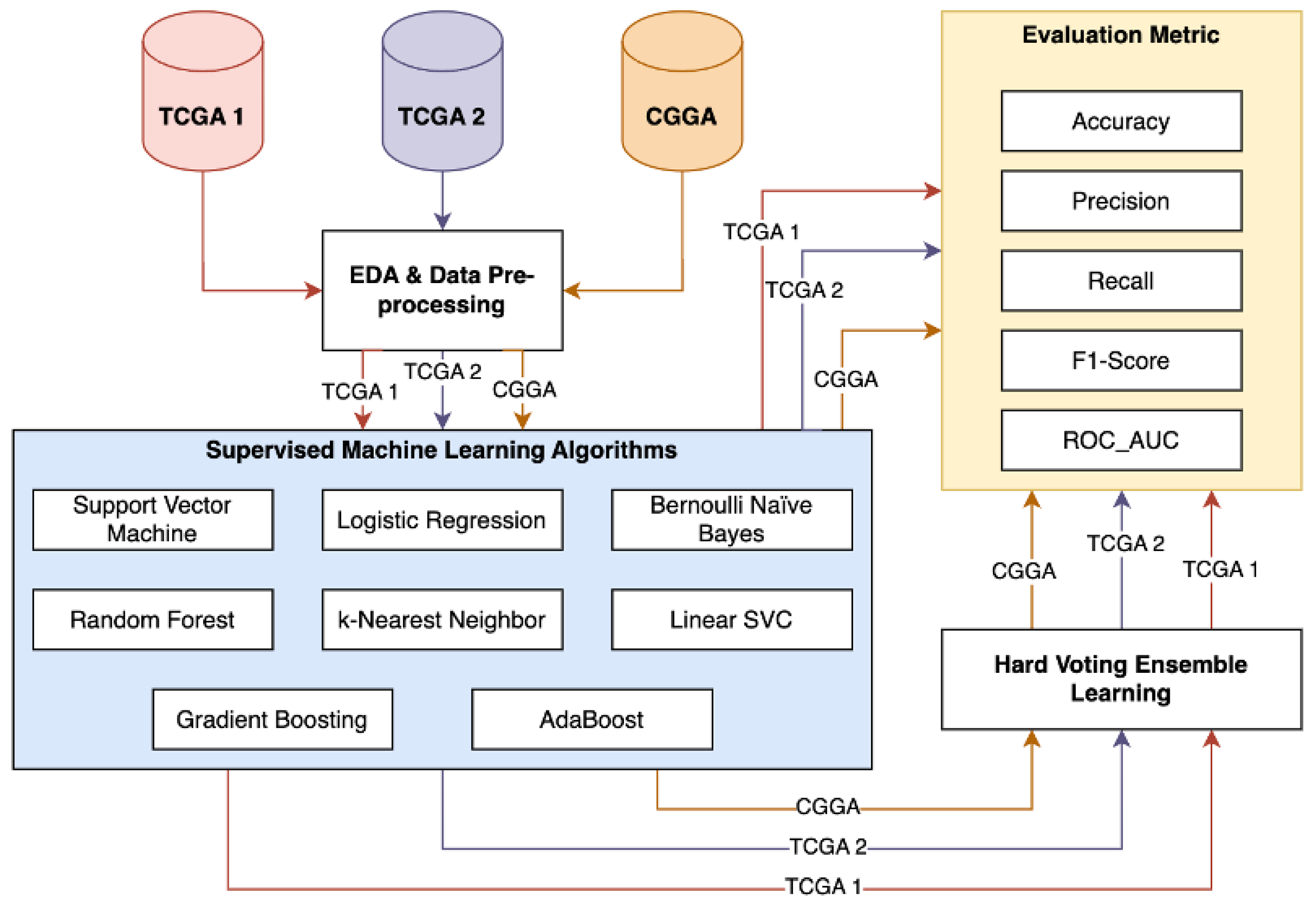
Figure 2.
Visual Representation of Random Forest [30].
Figure 2.
Visual Representation of Random Forest [30].
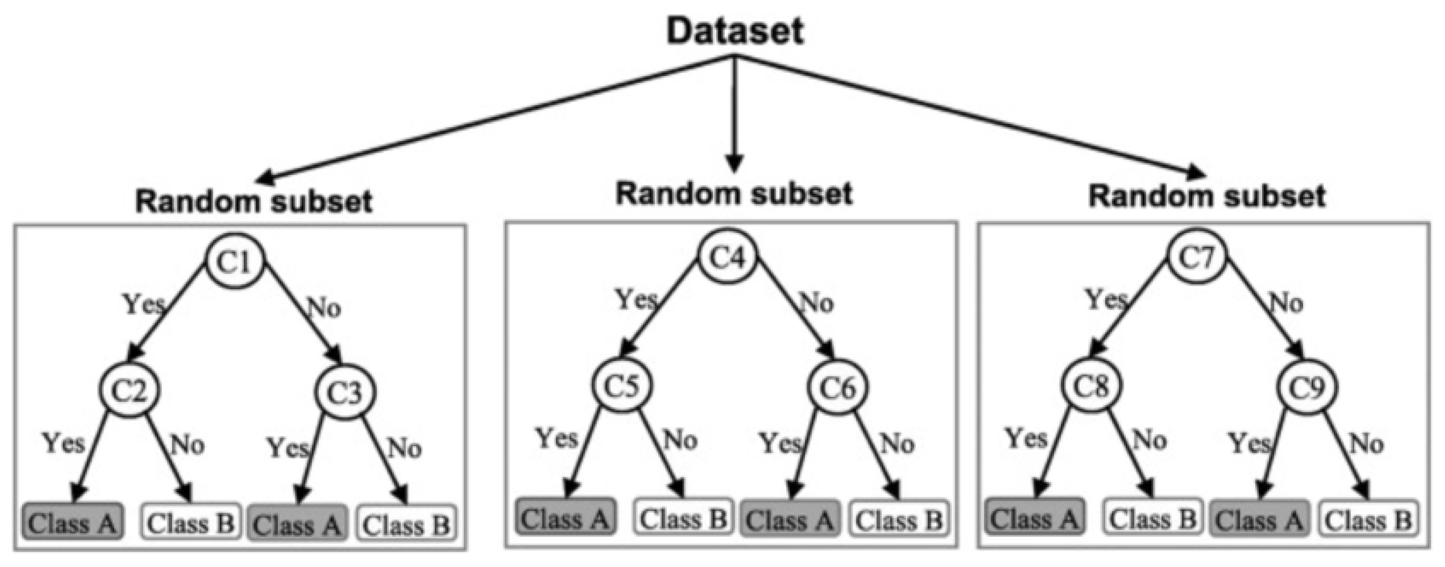
Figure 3.
Support Vector Machine and Hyperplane [31].
Figure 3.
Support Vector Machine and Hyperplane [31].
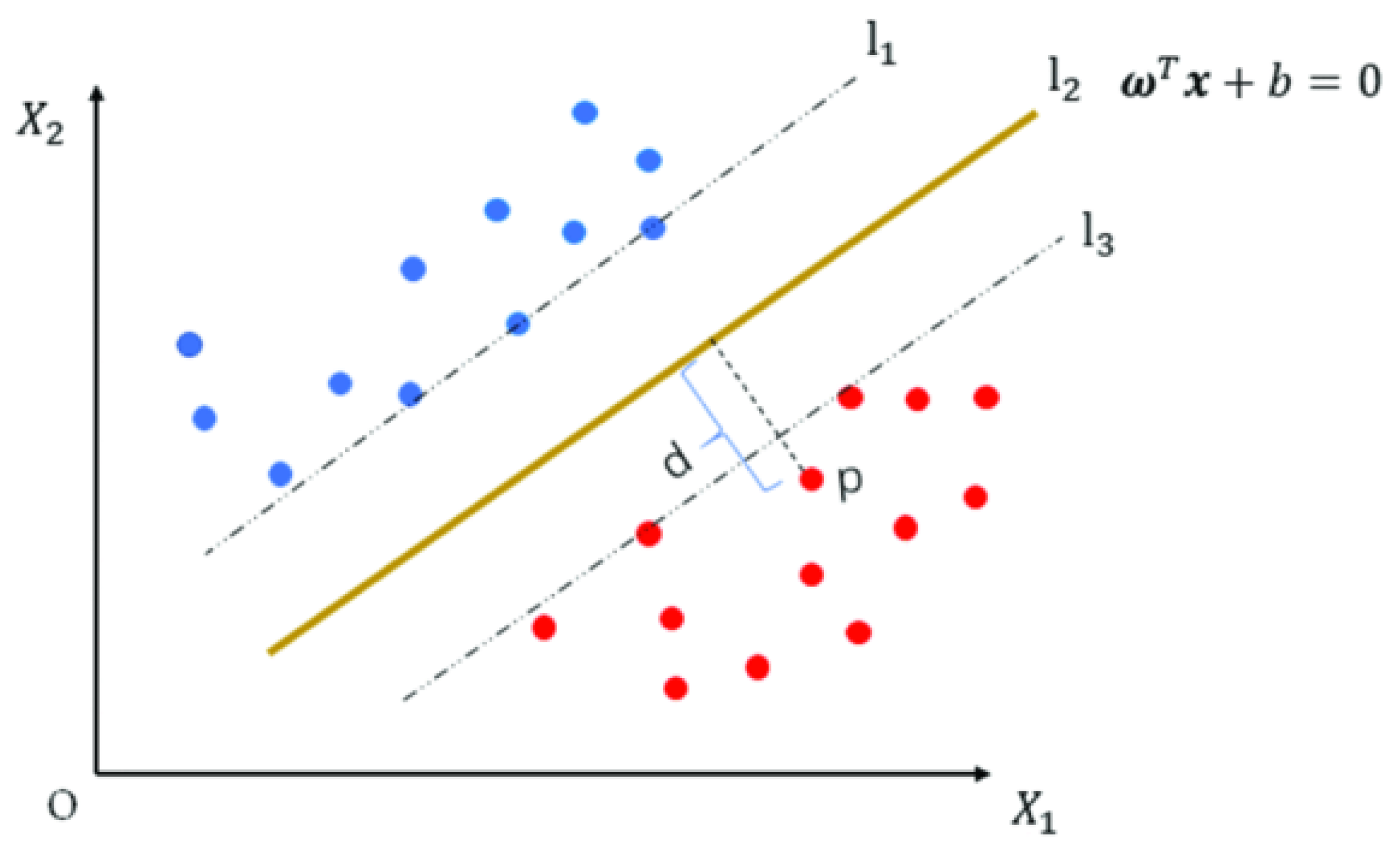
Figure 4.
The Effect of Regularization Parameter C in SVC [32], where the X-axis and the Y-axis represent the values of the regularization parameter C and model accuracy performance.
Figure 4.
The Effect of Regularization Parameter C in SVC [32], where the X-axis and the Y-axis represent the values of the regularization parameter C and model accuracy performance.
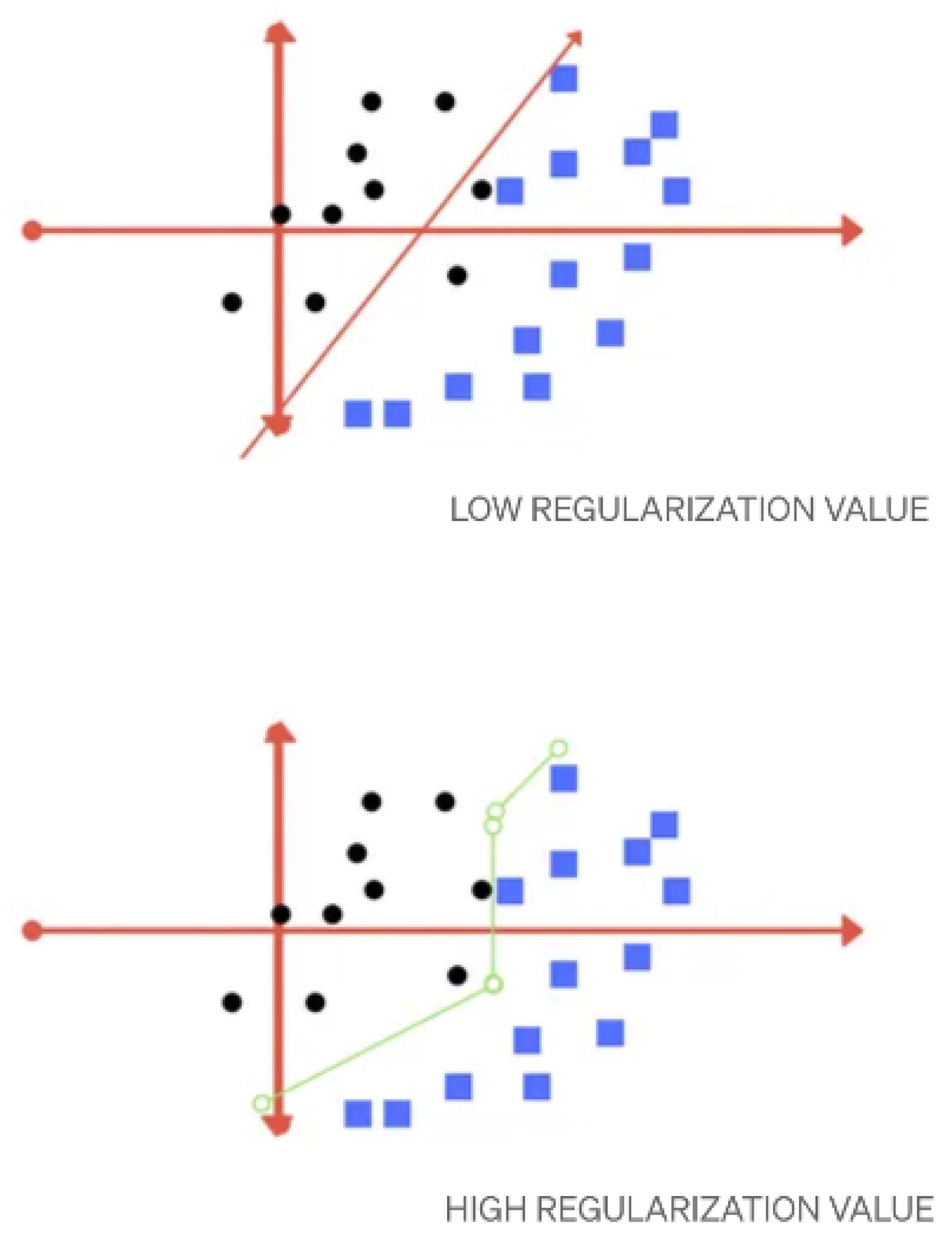
Figure 5.
Adaptive Boosting Process [31].
Figure 5.
Adaptive Boosting Process [31].
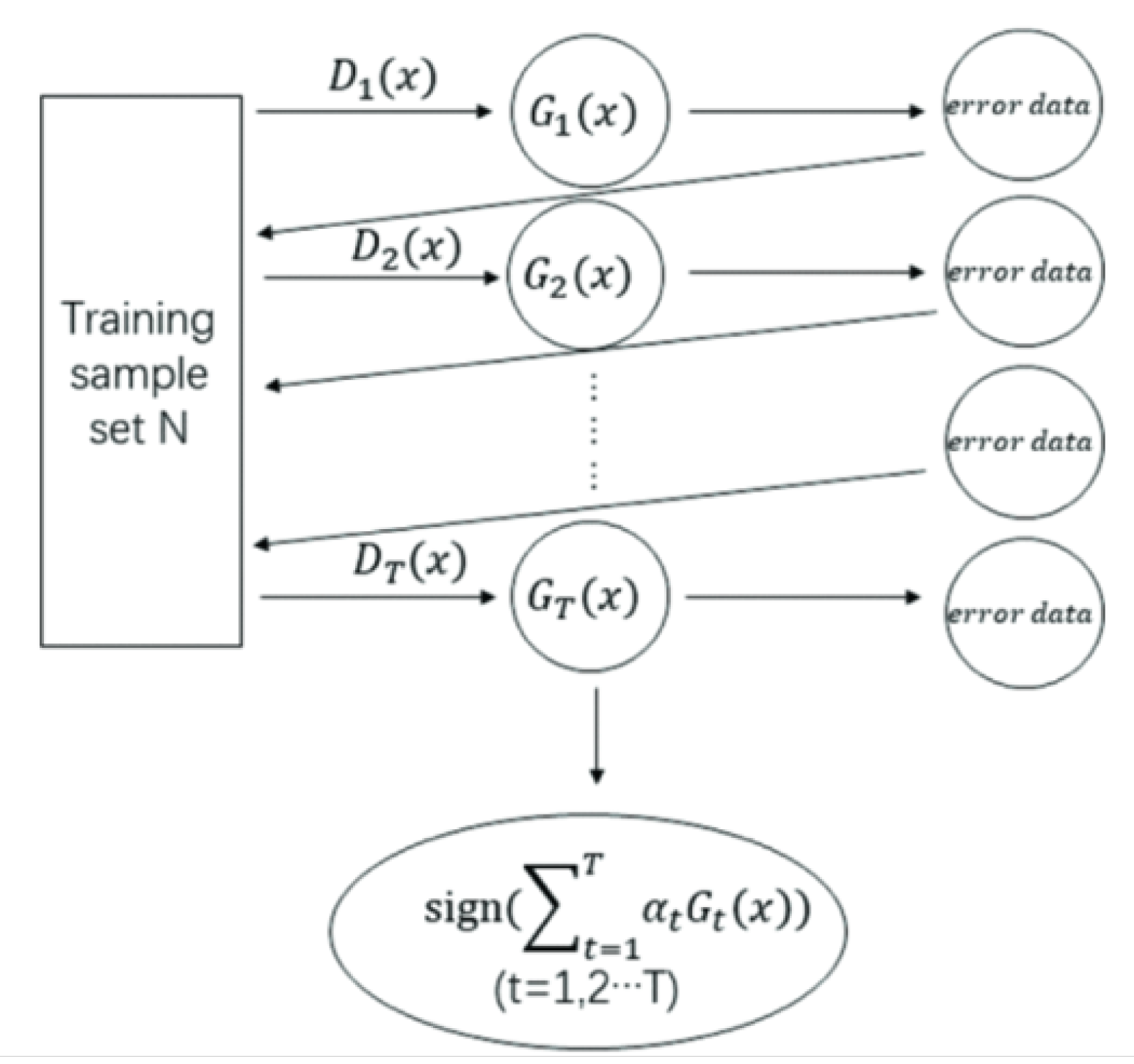
Figure 6.
Missing Values Visualisation of TCGA2 Dataset.
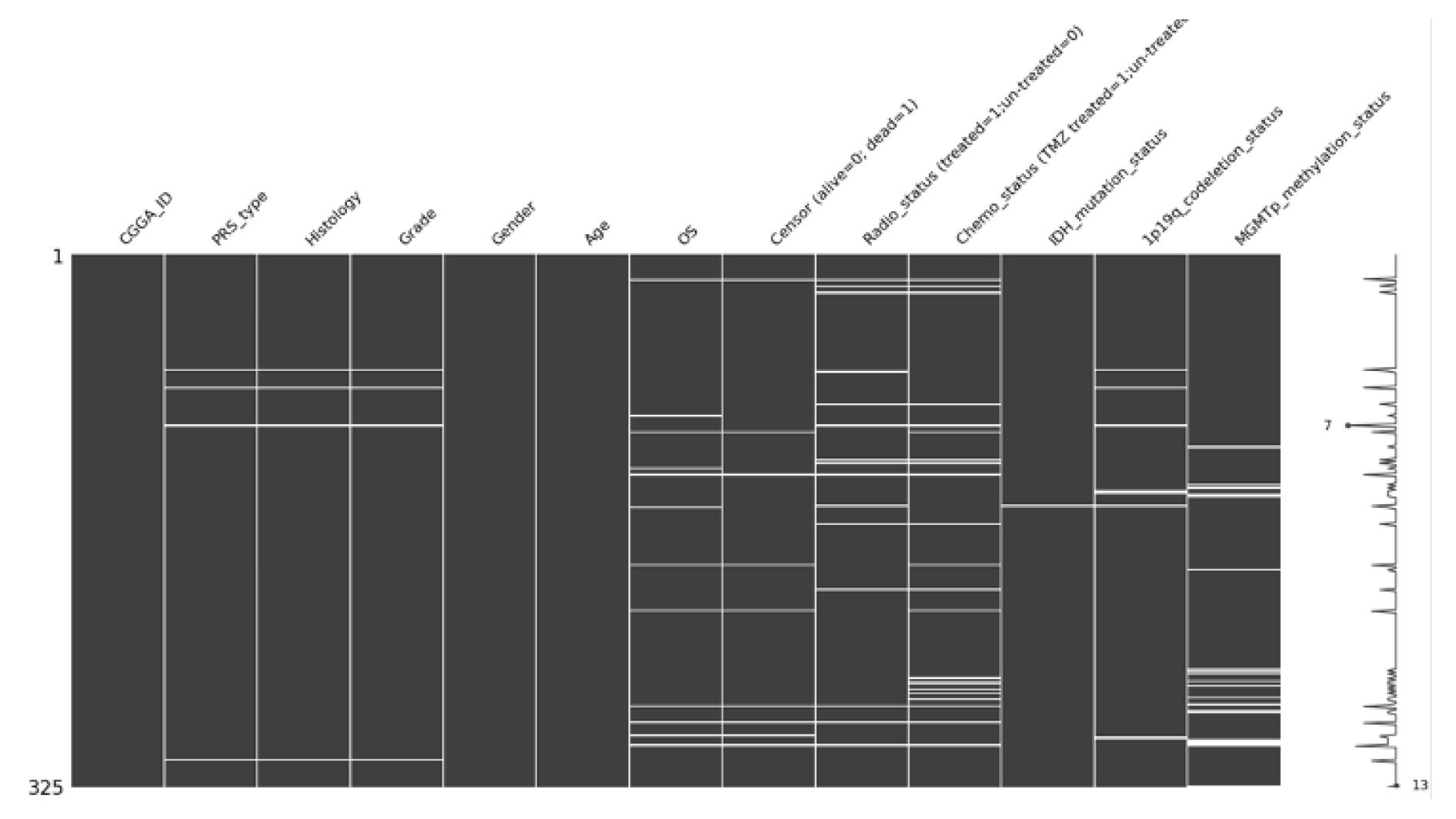
Figure 7.
Missing Values Visualisation of CGGA Dataset.
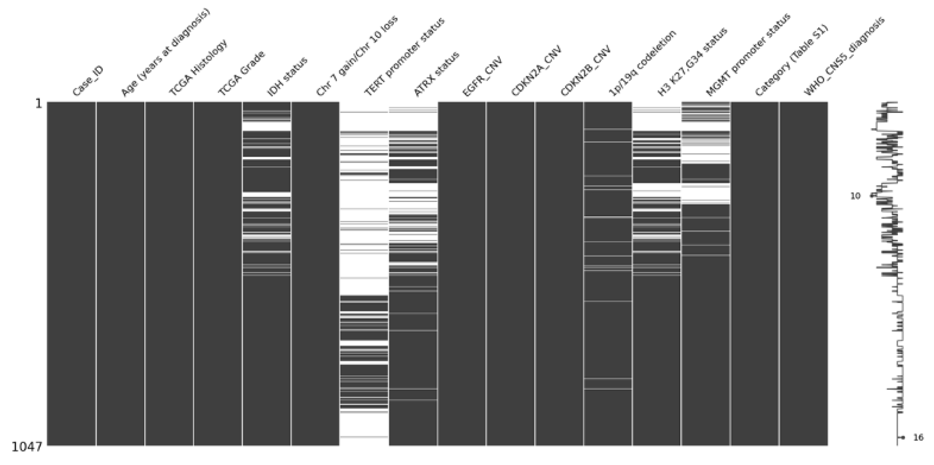
Figure 8.
Distribution of Age in All Dataset.
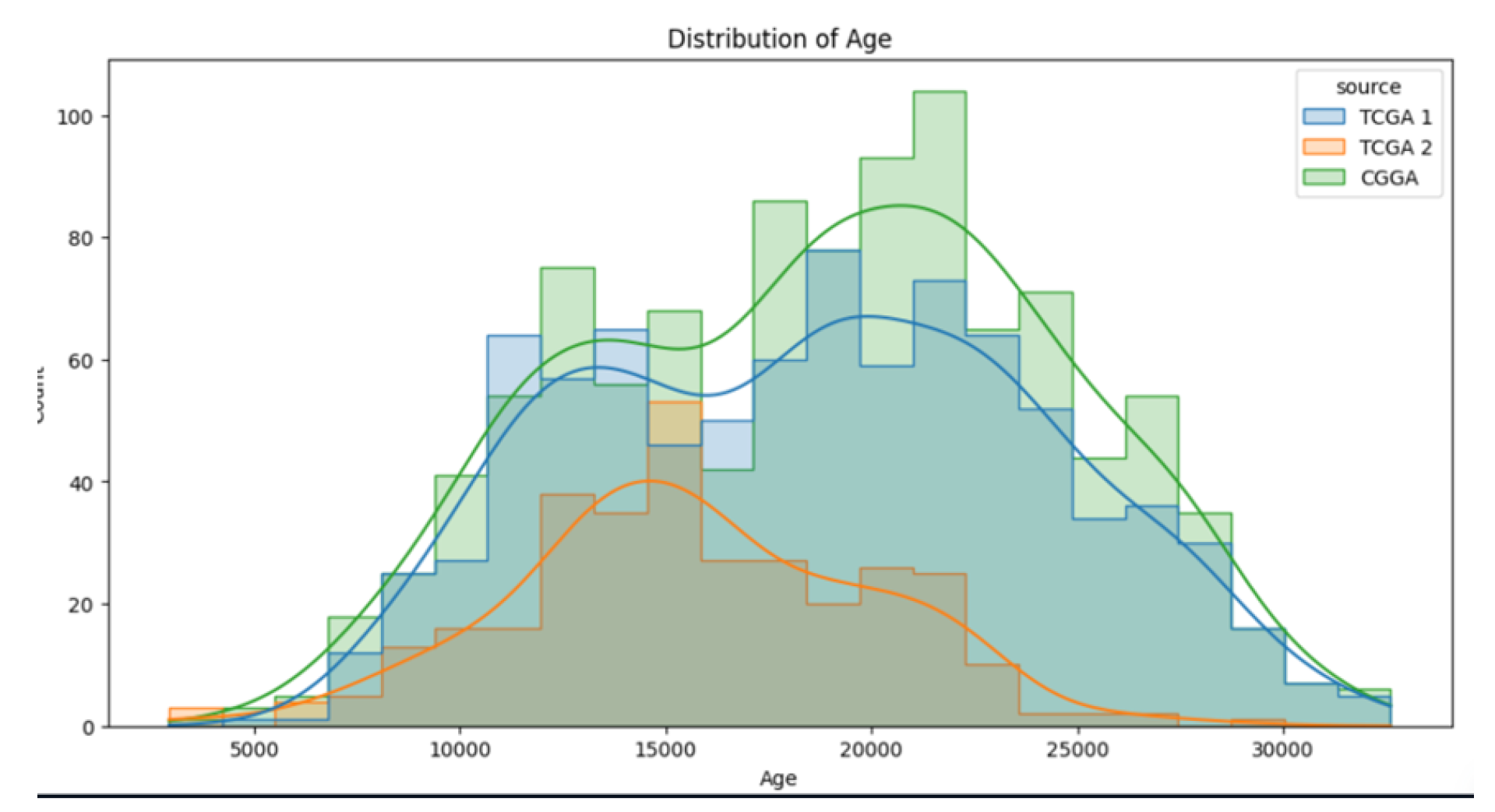
Figure 9.
Heatmap correlation for TCGA2.
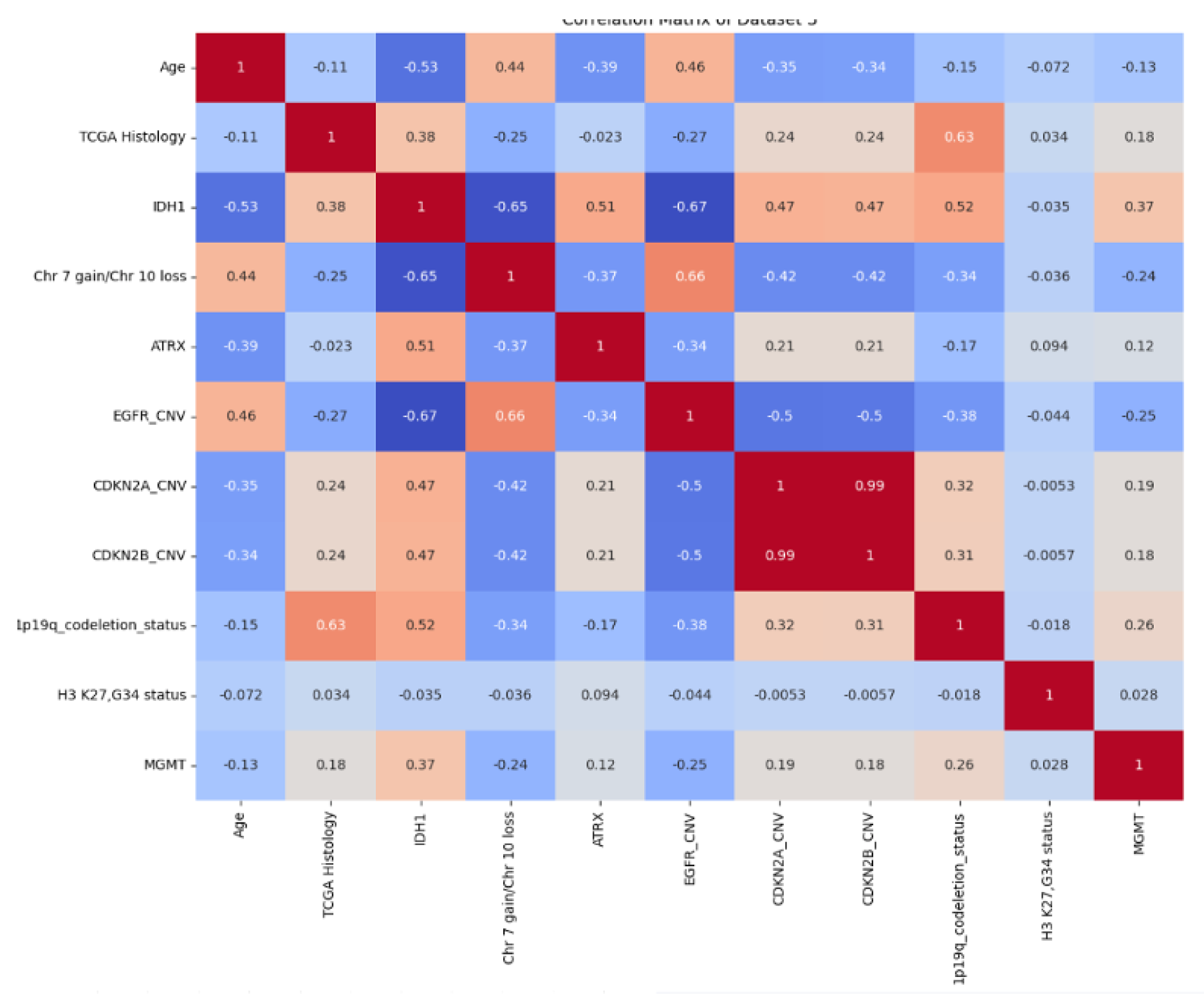
Figure 10.
Accuracy Result for TCGA 1 Test Set.

Figure 11.
Accuracy Result for CGGA Test Set.
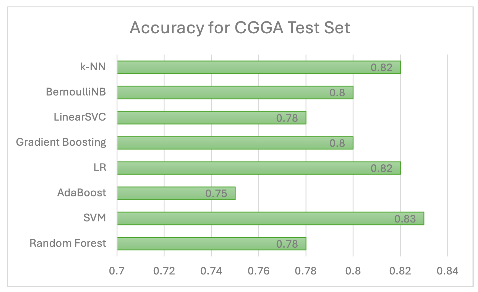
Figure 12.
Accuracy Result for TCGA 2 Test Set.
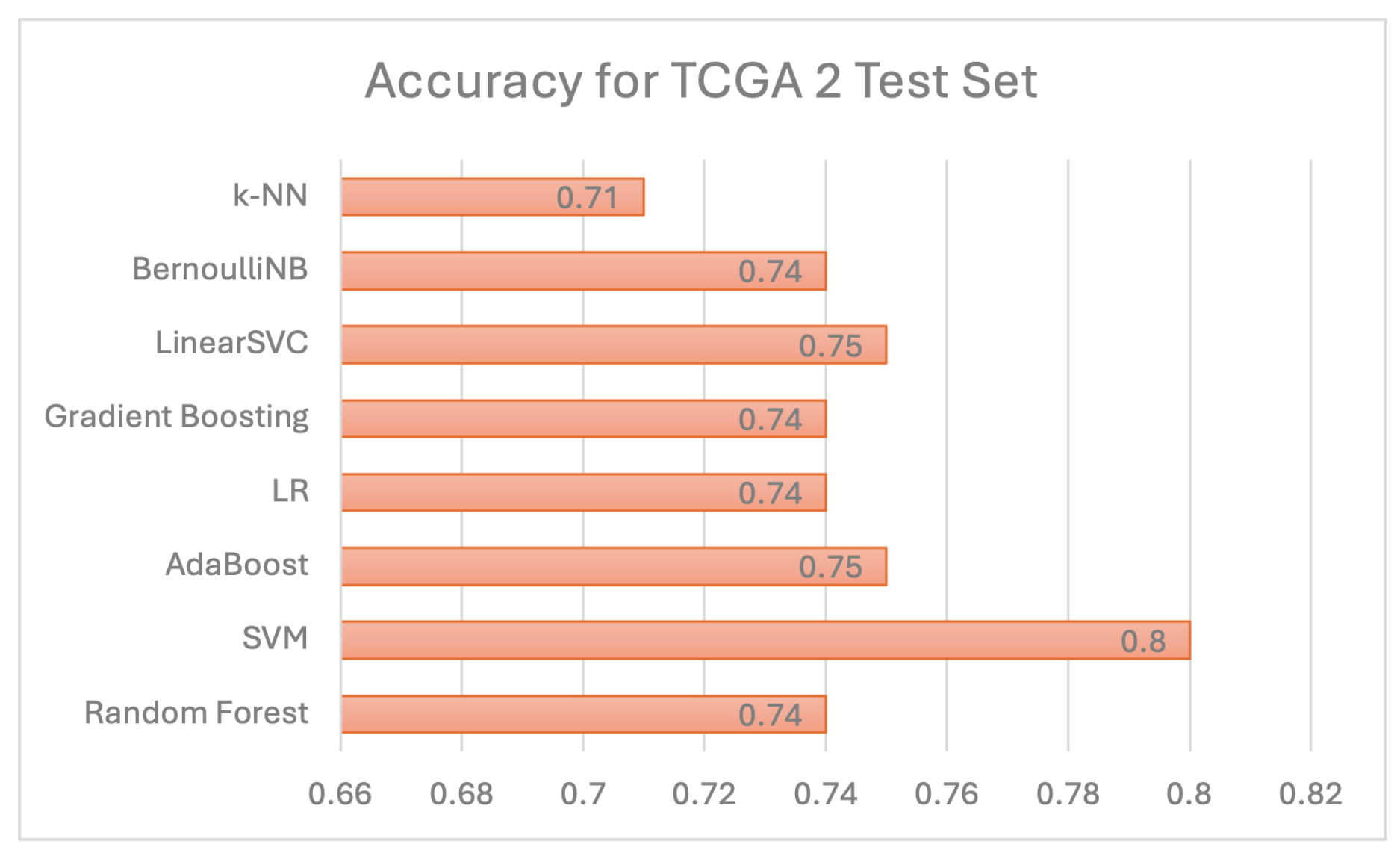
Figure 13.
Accuracy Result of Ensemble Learning for TCGA 1 Test Set.
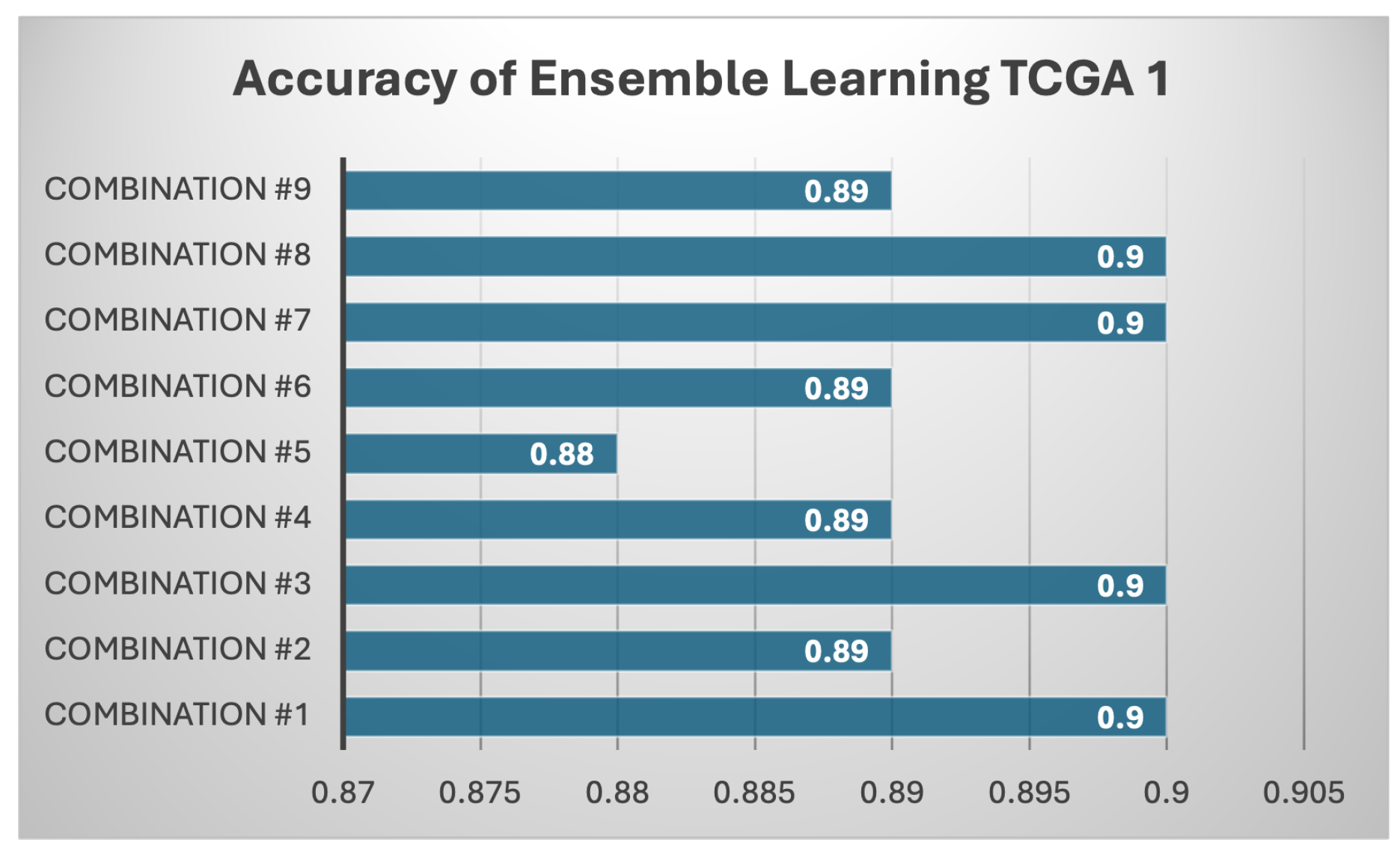
Figure 14.
Accuracy Result of Ensemble Learning for CGGA Test Set.
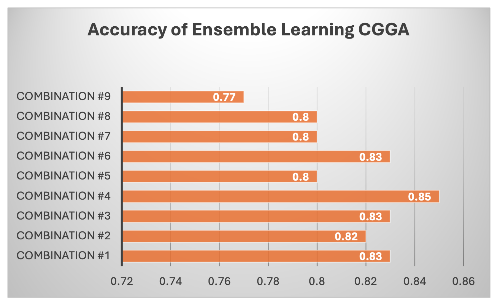
Figure 15.
Accuracy Result of Ensemble Learning for TCGA 2 Test Set.
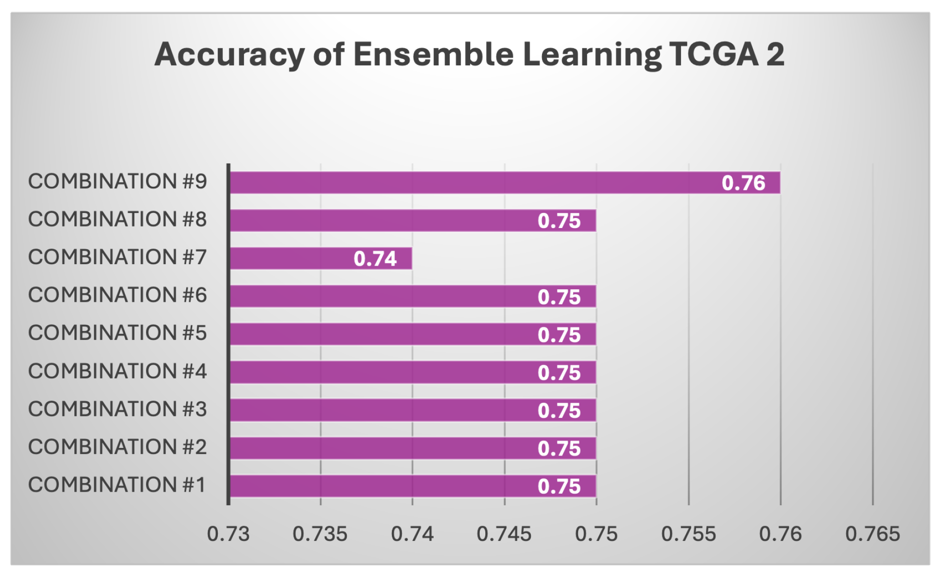
Figure 16.
ROC Curves of All Individual Models.
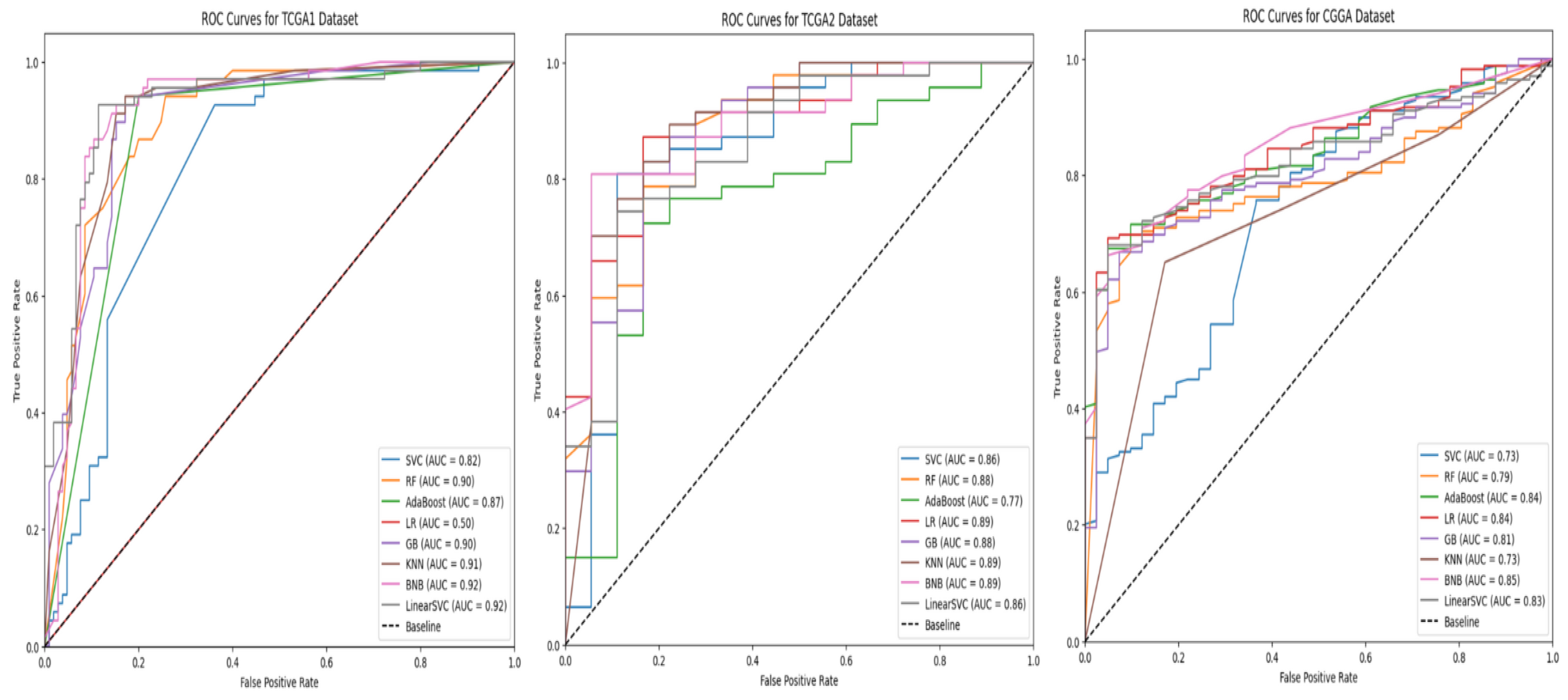
Figure 17.
Precision-Recall Curves of All Individual Models.
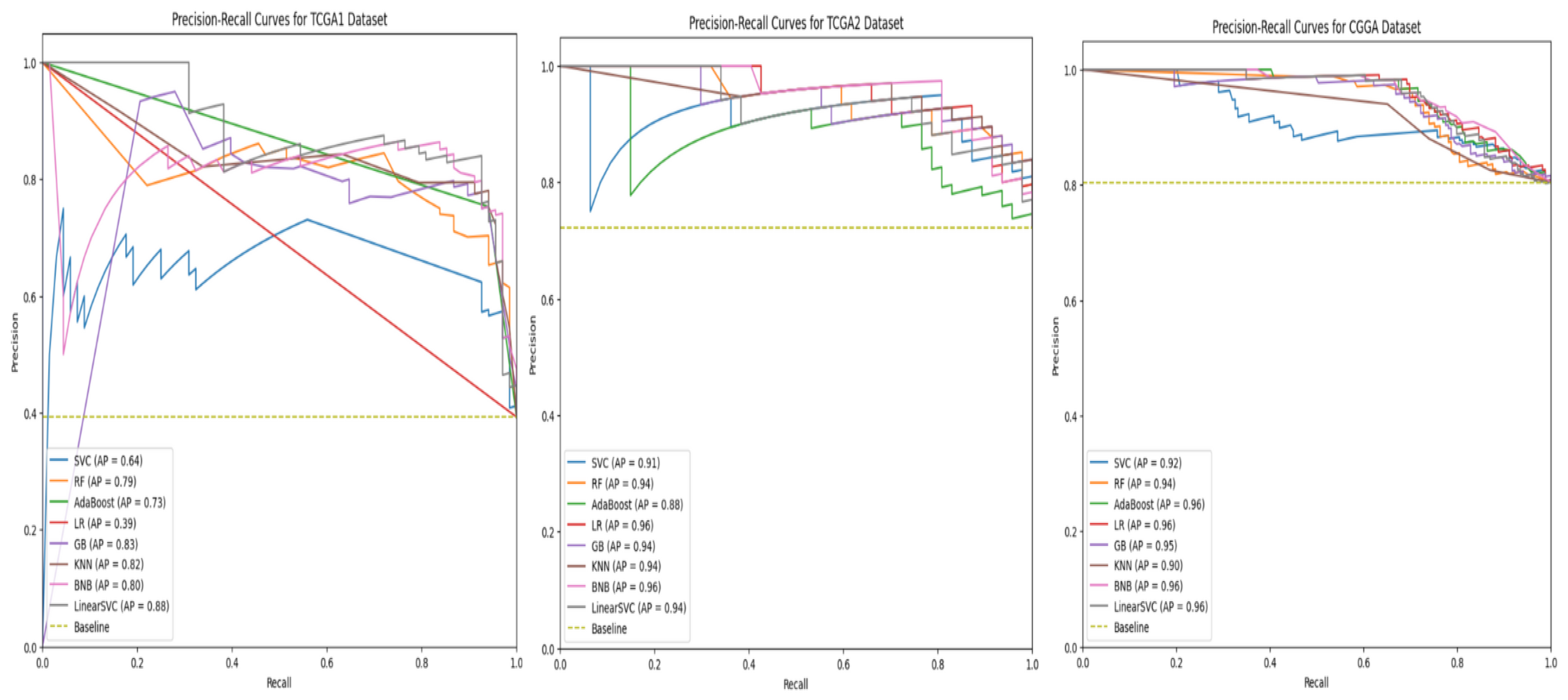
Figure 18.
Confusion Matrices of All Individual Models.
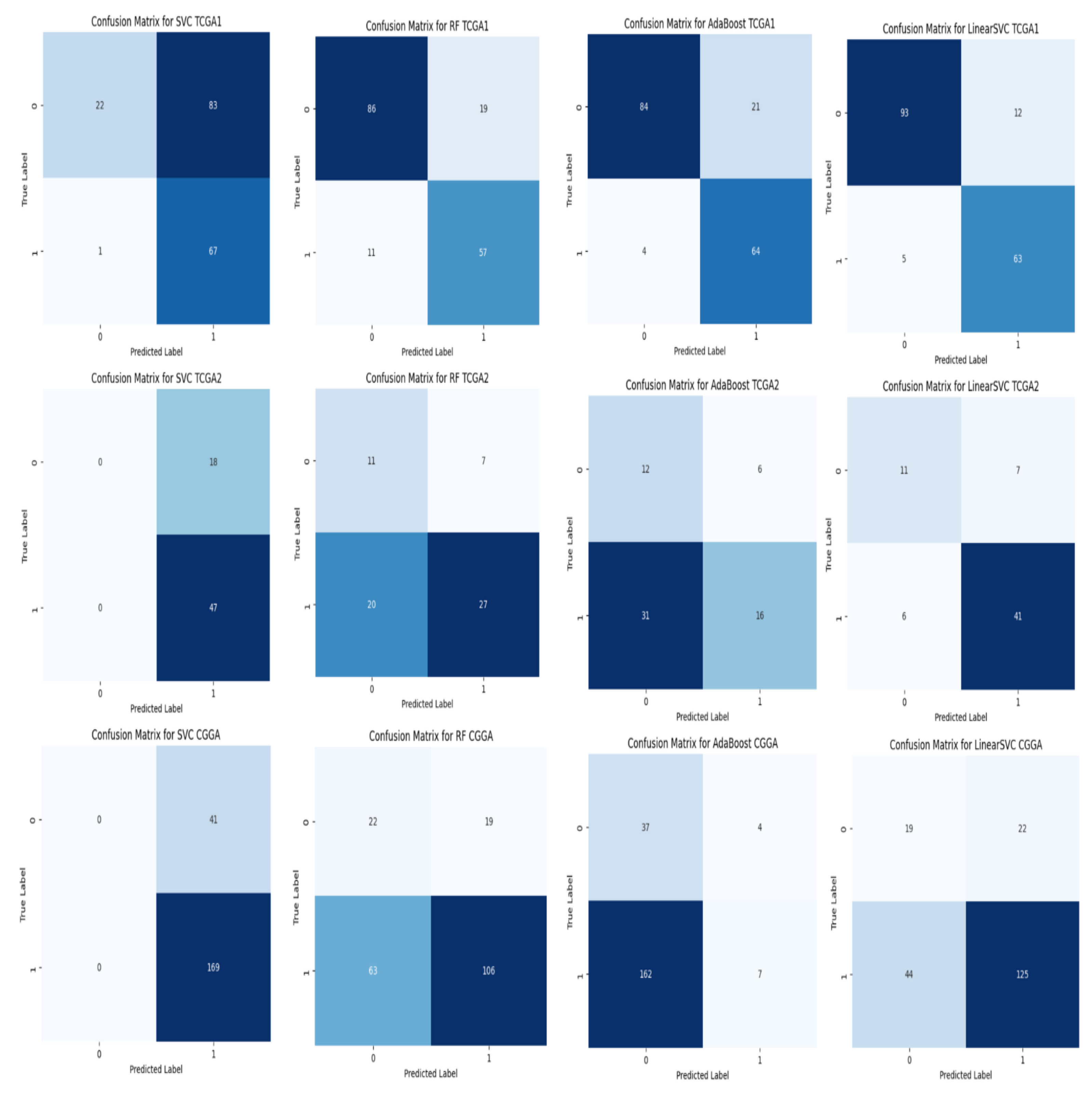
Figure 19.
Adaboost Mean SHAP Values for CGGA Dataset.
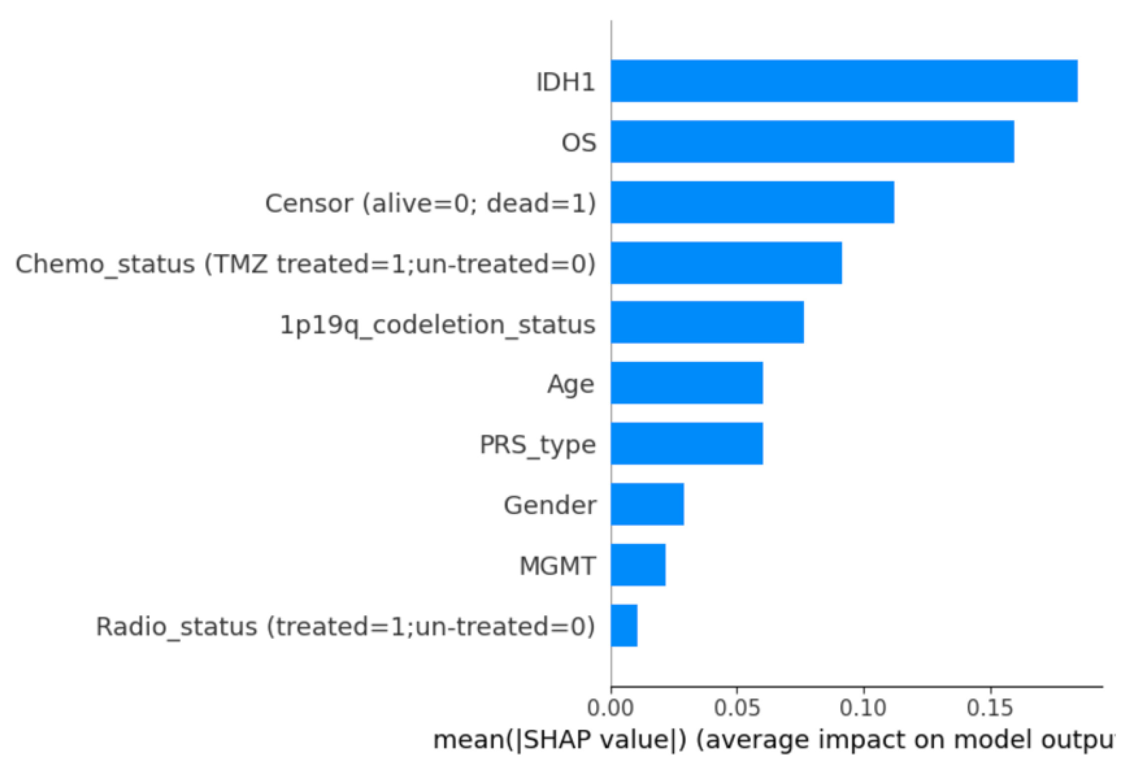
Figure 20.
Adaboost Mean SHAP Values for TCGA 1 Dataset.
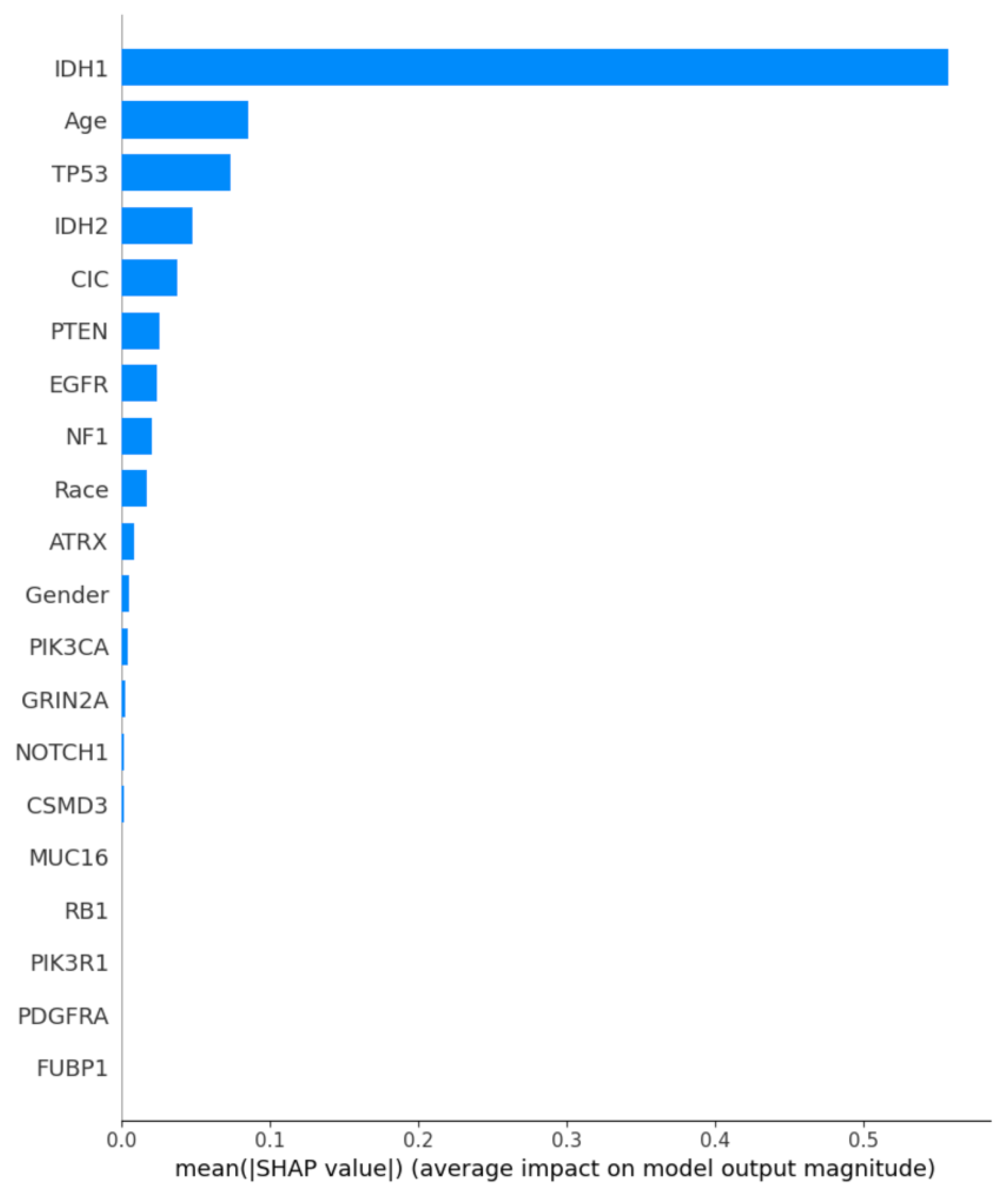
Table 1.
Summary of Related Works.
| Research Paper | Author(s) Name, Year and Reference No. | Best Model |
|---|---|---|
| Machine Learning Based Radiomics for Molecular Subtyping of Gliomas | Lu et al. (2018), [15] | Cubic SVM |
| Comparison of Feature Selection Methods and Machine Learning Classifiers for Radiomics Analysis in Glioma Grading | Sun et al. (2019), [21] | Multilayer Perceptron |
| Improved Glioma Grading Using Deep Convolutional Neural Networks | Gutta et al. (2021), [22] | Convolutional Neural Networks |
| Hierarchical Voting-Based Feature Selection and Ensemble Learning Model Scheme for Glioma Grading with Clinical and Molecular Characteristics | Tasci et al. (2022), [5] | Ensemble Learning Model–Soft Voting |
| Enhancing Glioma Grading Performance: A Comparative Study on Feature Selection Techniques and Ensemble Machine Learning | Noviandy et al. (2023), [16] | Ensemble Learning Model |
| Grade and Subtype Classification for Glioma Tumors using Clinical and Molecular Mutations | Oberoi et al. (2023), [17] | Logistic Regression |
| Gliomas Disease Prediction: An Optimized Ensemble Machine Learning-Based Approach | Thakur et al. (2023), [23] | KStar and SMOreg – Ensemble Learning Method |
| Enhanced Glioma Disease Prediction Through Ensemble-Optimized Machine Learning | Sriramoju and Srivastava (2024), [24] | Decision Tree and Random Forest – Ensemble Learning Method |
Table 3.
Features of structure of the 1st TCGA Dataset.
| Attributes | Description |
|---|---|
| Grade | Glioma grade of the corresponding patient |
| Project | The name of the genome atlas database |
| Case ID | Unique ID that corresponds to each patient |
| Gender | Gender of patient |
| Age at diagnosis | Age of patient |
| Primary Diagnosis | Types of glioma present |
| Race | Race of patient |
| IDH1 | Status of IDH1 mutation |
| TP53 | Status of TP53 mutation |
| ATRX | Status of ATRX mutation |
| PTEN | Status of PTEN mutation |
| EGFR | Status of EGFR mutation |
| CIC | Status of CIC mutation |
| MUC16 | Status of MUC16 mutation |
| PIK3CA | Status of PIK3CA mutation |
| NF1 | Status of NF1 mutation |
| PIK3R1 | Status of PIK3R1 mutation |
| FUBP1 | Status of FUBP1 mutation |
| RB1 | Status of RB1 mutation |
| NOTCH1 | Status of NOTCH1 mutation |
| BCOR | Status of BCOR mutation |
| CSMD3 | Status of CSMD3 mutation |
| SMARCA4 | Status of SMARCA4 mutation |
| GRIN2A | Status of GRIN2A mutation |
| IDH2 | Status of IDH2 mutation |
| FAT4 | Status of FAT4 mutation |
| PDGFRA | Status of PDGFRA mutation |
Table 4.
TCGA 2nd Dataset Description.
| Attributes | Description |
|---|---|
| Case ID | Unique ID that corresponds to each patient |
| Age (years at diagnosis) | Age of patients |
| TCGA Histology | Types of glioma present |
| TCGA Grade | Glioma grade of the corresponding patient |
| IDH1 Status | Status of IDH1 mutation |
| Chr 7 gain/Chr 10 loss | Status of chromosome 7 gain and 10 loss combination |
| TERT promoter status | Status of TERT mutation |
| ATRX status | Status of ATRX mutation |
| EGFR CNV | Number of CNVs in the EGFR gene |
| CDKN2A CNV | Number of CNVs in the CDKN2A gene |
| CDKN2B CNV | Number of CNVs in the CDKN2B gene |
| 1p/19q codeletion | Status of 1p/19q chromosomal codeletion |
| H3 K27, G34 status | Status of H3 K27 and H3 G34 mutations |
| MGMT promoter status | Status of MGMT mutation |
| Category (Table S1) | Description of the glioma combination |
| WHO CNS5 diagnosis | Glioma grade by the World Health Organization |
Table 5.
CGGA Dataset Description.
| Attributes | Description |
|---|---|
| CGGA ID | Unique ID that corresponds to each patient |
| PRS type | Primary or recurrent glioma |
| Histology | Types of glioma present |
| Grade | Glioma grade by WHO |
| Gender | Gender of patient |
| Age | Age of patient |
| OS | Overall survival of patient |
| Censor (alive=0; dead=1) | Dead or alive status |
| Radio status (treated=1; untreated=0) | Radiation therapy treatment status |
| Chemo status (TMZ treated=1; untreated=0) | Chemotherapy treatment status |
| IDH mutation status | IDH1 and IDH2 mutation status |
| 1p19q codeletion status | Status of 1p/19q chromosomal codeletion |
| MGMTp methylation status | MGMT methylation status |
Table 6.
Results of Individual ML Algorithms.
| Dataset | Accuracy | Precision | Recall | F1 | ROCAUC |
|---|---|---|---|---|---|
| Random Forest | |||||
| TCGA 1 | 0.83 ± 0.02 | 0.75 ± 0.01 | 0.84 ± 0.02 | 0.79 ± 0.01 | 0.83 ± 0.01 |
| CGGA | 0.78 ± 0.01 | 0.88 ± 0.01 | 0.81 ± 0.01 | 0.84 ± 0.01 | 0.77 ± 0.01 |
| TCGA 2 | 0.74 ± 0.02 | 0.88 ± 0.01 | 0.79 ± 0.01 | 0.83 ± 0.01 | 0.66 ± 0.02 |
| Support Vector Machine | |||||
| TCGA 1 | 0.51 ± 0.02 | 0.45 ± 0.01 | 0.99 ± 0.01 | 0.61 ± 0.01 | 0.60 ± 0.01 |
| CGGA | 0.83 ± 0.01 | 0.85 ± 0.01 | 0.94 ± 0.01 | 0.89 ± 0.01 | 0.75 ± 0.01 |
| TCGA 2 | 0.80 ± 0.01 | 0.85 ± 0.01 | 0.92 ± 0.01 | 0.88 ± 0.01 | 0.62 ± 0.01 |
| AdaBoost | |||||
| TCGA 1 | 0.86 ± 0.01 | 0.75 ± 0.01 | 0.94 ± 0.01 | 0.84 ± 0.01 | 0.87 ± 0.01 |
| CGGA | 0.75 ± 0.01 | 0.86 ± 0.01 | 0.79 ± 0.01 | 0.82 ± 0.01 | 0.73 ± 0.01 |
| TCGA 2 | 0.75 ± 0.02 | 0.93 ± 0.01 | 0.75 ± 0.01 | 0.83 ± 0.01 | 0.75 ± 0.01 |
| Logistic Regression | |||||
| TCGA 1 | 0.61 ± 0.02 | 0.00 ± 0.00 | 0.00 ± 0.00 | 0.00 ± 0.00 | 0.50 ± 0.01 |
| CGGA | 0.82 ± 0.01 | 0.93 ± 0.01 | 0.81 ± 0.01 | 0.86 ± 0.01 | 0.82 ± 0.01 |
| TCGA 2 | 0.74 ± 0.02 | 0.95 ± 0.01 | 0.71 ± 0.01 | 0.81 ± 0.01 | 0.78 ± 0.01 |
| Gradient Boosting | |||||
| TCGA 1 | 0.86 ± 0.01 | 0.78 ± 0.01 | 0.90 ± 0.01 | 0.84 ± 0.01 | 0.87 ± 0.01 |
| CGGA | 0.80 ± 0.01 | 0.93 ± 0.01 | 0.79 ± 0.01 | 0.85 ± 0.01 | 0.81 ± 0.01 |
| TCGA 2 | 0.74 ± 0.02 | 0.88 ± 0.01 | 0.79 ± 0.01 | 0.82 ± 0.01 | 0.66 ± 0.02 |
| Linear SVC | |||||
| TCGA 1 | 0.90 ± 0.01 | 0.84 ± 0.01 | 0.93 ± 0.01 | 0.88 ± 0.01 | 0.91 ± 0.01 |
| CGGA | 0.78 ± 0.01 | 0.87 ± 0.01 | 0.83 ± 0.01 | 0.85 ± 0.01 | 0.75 ± 0.01 |
| TCGA 2 | 0.75 ± 0.02 | 0.96 ± 0.01 | 0.72 ± 0.01 | 0.82 ± 0.01 | 0.80 ± 0.01 |
| Bernoulli Naïve Bayes | |||||
| TCGA 1 | 0.88 ± 0.01 | 0.80 ± 0.01 | 0.93 ± 0.01 | 0.96 ± 0.01 | 0.89 ± 0.01 |
| CGGA | 0.80 ± 0.01 | 0.89 ± 0.01 | 0.83 ± 0.01 | 0.86 ± 0.01 | 0.78 ± 0.01 |
| TCGA 2 | 0.74 ± 0.02 | 0.95 ± 0.01 | 0.72 ± 0.01 | 0.82 ± 0.01 | 0.78 ± 0.01 |
| K-Nearest Neighbors | |||||
| TCGA 1 | 0.86 ± 0.01 | 0.78 ± 0.01 | 0.91 ± 0.01 | 0.84 ± 0.01 | 0.87 ± 0.01 |
| CGGA | 0.82 ± 0.01 | 0.93 ± 0.01 | 0.81 ± 0.01 | 0.86 ± 0.01 | 0.82 ± 0.01 |
| TCGA 2 | 0.71 ± 0.02 | 0.88 ± 0.01 | 0.74 ± 0.01 | 0.80 ± 0.01 | 0.66 ± 0.02 |
Table 7.
Results of Each Set of Ensemble Learning.
| Dataset | Accuracy | Precision | Recall | F1 | ROC AUC |
|---|---|---|---|---|---|
| LinearSVC + AdaBoost + BNB + k-NN + RF | |||||
| TCGA 1 | 0.90 ± 0.01 | 0.84 ± 0.01 | 0.93 ± 0.01 | 0.88 ± 0.01 | 0.91 ± 0.01 |
| CGGA | 0.83 ± 0.01 | 0.93 ± 0.01 | 0.83 ± 0.01 | 0.88 ± 0.01 | 0.83 ± 0.01 |
| TCGA 2 | 0.75 ± 0.01 | 0.94 ± 0.01 | 0.73 ± 0.01 | 0.83 ± 0.01 | 0.77 ± 0.01 |
| LinearSVC + AdaBoost + BNB + RF | |||||
| TCGA 1 | 0.89 ± 0.01 | 0.84 ± 0.01 | 0.90 ± 0.01 | 0.87 ± 0.01 | 0.89 ± 0.01 |
| CGGA | 0.82 ± 0.01 | 0.93 ± 0.01 | 0.81 ± 0.01 | 0.86 ± 0.01 | 0.82 ± 0.01 |
| TCGA 2 | 0.75 ± 0.01 | 0.95 ± 0.01 | 0.73 ± 0.01 | 0.82 ± 0.01 | 0.78 ± 0.01 |
| LinearSVC + AdaBoost + BNB + k-NN | |||||
| TCGA 1 | 0.90 ± 0.01 | 0.84 ± 0.01 | 0.93 ± 0.01 | 0.88 ± 0.01 | 0.91 ± 0.01 |
| CGGA | 0.83 ± 0.01 | 0.95 ± 0.01 | 0.81 ± 0.01 | 0.87 ± 0.01 | 0.85 ± 0.01 |
| TCGA 2 | 0.75 ± 0.01 | 0.95 ± 0.01 | 0.72 ± 0.01 | 0.82 ± 0.01 | 0.78 ± 0.01 |
| LinearSVC + k-NN + BNB + RF | |||||
| TCGA 1 | 0.89 ± 0.01 | 0.84 ± 0.01 | 0.90 ± 0.01 | 0.87 ± 0.01 | 0.89 ± 0.01 |
| CGGA | 0.85 ± 0.01 | 0.95 ± 0.01 | 0.83 ± 0.01 | 0.89 ± 0.01 | 0.86 ± 0.01 |
| TCGA 2 | 0.75 ± 0.01 | 0.97 ± 0.01 | 0.71 ± 0.01 | 0.82 ± 0.01 | 0.81 ± 0.01 |
| AdaBoost + k-NN + BNB + RF | |||||
| TCGA 1 | 0.88 ± 0.01 | 0.83 ± 0.01 | 0.88 ± 0.01 | 0.86 ± 0.01 | 0.88 ± 0.01 |
| CGGA | 0.80 ± 0.01 | 0.93 ± 0.01 | 0.79 ± 0.01 | 0.85 ± 0.01 | 0.81 ± 0.01 |
| TCGA 2 | 0.75 ± 0.01 | 0.95 ± 0.01 | 0.73 ± 0.01 | 0.83 ± 0.01 | 0.79 ± 0.01 |
| AdaBoost + k-NN + LinearSVC + RF | |||||
| TCGA 1 | 0.89 ± 0.01 | 0.84 ± 0.01 | 0.90 ± 0.01 | 0.87 ± 0.01 | 0.89 ± 0.01 |
| CGGA | 0.83 ± 0.01 | 0.95 ± 0.01 | 0.79 ± 0.01 | 0.86 ± 0.01 | 0.84 ± 0.01 |
| TCGA 2 | 0.75 ± 0.01 | 0.96 ± 0.01 | 0.72 ± 0.01 | 0.82 ± 0.01 | 0.80 ± 0.01 |
| LinearSVC + AdaBoost + k-NN | |||||
| TCGA 1 | 0.90 ± 0.01 | 0.84 ± 0.01 | 0.93 ± 0.01 | 0.88 ± 0.01 | 0.91 ± 0.01 |
| CGGA | 0.80 ± 0.01 | 0.90 ± 0.01 | 0.81 ± 0.01 | 0.85 ± 0.01 | 0.79 ± 0.01 |
| TCGA 2 | 0.74 ± 0.01 | 0.94 ± 0.01 | 0.73 ± 0.01 | 0.82 ± 0.01 | 0.77 ± 0.01 |
| LinearSVC + AdaBoost + BNB | |||||
| TCGA 1 | 0.90 ± 0.01 | 0.84 ± 0.01 | 0.93 ± 0.01 | 0.88 ± 0.01 | 0.91 ± 0.01 |
| CGGA | 0.80 ± 0.01 | 0.90 ± 0.01 | 0.83 ± 0.01 | 0.86 ± 0.01 | 0.78 ± 0.01 |
| TCGA 2 | 0.75 ± 0.01 | 0.95 ± 0.01 | 0.73 ± 0.01 | 0.83 ± 0.01 | 0.78 ± 0.01 |
| LinearSVC + k-NN + BNB | |||||
| TCGA 1 | 0.90 ± 0.01 | 0.84 ± 0.01 | 0.93 ± 0.01 | 0.88 ± 0.01 | 0.91 ± 0.01 |
| CGGA | 0.81 ± 0.01 | 0.90 ± 0.01 | 0.82 ± 0.01 | 0.86 ± 0.01 | 0.78 ± 0.01 |
| TCGA 2 | 0.75 ± 0.01 | 0.95 ± 0.01 | 0.73 ± 0.01 | 0.83 ± 0.01 | 0.78 ± 0.01 |
Disclaimer/Publisher’s Note: The statements, opinions and data contained in all publications are solely those of the individual author(s) and contributor(s) and not of MDPI and/or the editor(s). MDPI and/or the editor(s) disclaim responsibility for any injury to people or property resulting from any ideas, methods, instructions or products referred to in the content. |
© 2024 by the authors. Licensee MDPI, Basel, Switzerland. This article is an open access article distributed under the terms and conditions of the Creative Commons Attribution (CC BY) license (https://creativecommons.org/licenses/by/4.0/).
Copyright: This open access article is published under a Creative Commons CC BY 4.0 license, which permit the free download, distribution, and reuse, provided that the author and preprint are cited in any reuse.


