Topology of Locally and Non-Locally Generalized Derivatives

1. Introduction

Physically, a derivative can be interpreted as the rate of change of one continuous quantity compared to another, measured at space-time scale, which can be considered "infinitesimal". On the other hand, scientific developments in the last 100 years indicate that the use of functions, non-differentiable in this classical sense, can not be avoided when modeling natural phenomena. For instance, the idealized process of diffusing particles, the Wiener process, has non-differentiable paths. The Ornstein–Uhlenbeck process, used in the kinetic theory of gasses assumes non-differentiable velocity fields [1]. Turbulence can also exhibit non-differentiable acceleration field [2]. In a closely related manner, the paths in Feynman’s path-integral approach to quantum mechanics are non-differentiable [3]. The deterministic approach of scale relativity theory, introduced by Nottale [4] also assumes non-differentiability of the fundamental space-time manifold. Such and other models can be viewed as an idealization indicating that the actual dynamics plays out at time-scales which are incommensurable with the scale of observation of the process.

Discontinuities in spatial gradients are essential elements of the models of certain physical phenomena. Shock waves in fluid dynamics represent abrupt changes in pressure, density, and velocity. These changes lead to discontinuities in the derivatives of the flow variables [5]. The behavior of gases in phase transitions, such as the transition from gas to liquid state, can exhibit discontinuous derivatives in thermodynamic quantities like pressure and volume.

Fractals are geometrical objects featuring both self-similarity and non- differentiability. Fractal shapes are ubiquitous in nature [6]. Fractals are closely related to mathematical "monsters", such as the non-differentiable functions of Weierstrass, Takagi, Bolzano, etc. More "well-behaving" but still surprising are the singular functions of Cantor-Lebesgue [7], Minkowski and the Smith-Cantor-Volterra function [8], which grow only on disconnected "Cantor dust" type of sets. Such functions arise in a variety of problems – ranging from number theory [9,10] to probability [11] Such concepts have been used for example in modeling fractures and their mechanics [12]. With the rising awareness about fractals some extensions of calculus, e.g., of derivatives, have been put forward in order to describe such phenomena. All these objects present challenges for their description by the differential calculus apparatus – that is by derivatives and integrals of functions.

Purely mathematically, the derivatives can be generalized in several ways. For example, a derivative can be defined in as the limit of difference quotients on the accumulation sets of points [13, ch 3, p. 105]. This is a profound definition, which can be immediately brought on Cantor sets in the scope of fractal calculus[14,15]. On the other hand, the question of the continuity on compact intervals of so-defined functions requires further specification.

From a different perspective, assuming the usual topology of the real line, the derivatives can be generalized also by a fractionalization using the formal substitution $\Delta x\to {\left(\Delta x\right)}^{\beta }$ in the difference quotient. This leads to the concept of fractional velocity as defined by Cherbit [16]. This quasi-differential operator was introduced by analogy with the Hausdorff dimension as a tool to study the fractal phenomena and physical processes for which instantaneous velocity was not well-defined 1. Several works have demonstrated that the resulting image functions are only trivially continuous in the usual topology of the real line [17,18]. On the other hand, interesting applications to singular functions have been also demonstrated [19]. It is customary in contemporary literature to formally substitute derivatives with non-local fractional-order operators, such as the Riemann-Liouville differintegral. In the present contribution I do not argue in favor of the formal fractionalization approach. Hristov convincingly argues that the appropriate fractionalization approach should start from the fractionalization of constitutive relations [20].

The definition of local fractional derivative introduced by Kolwankar and Gangal [21] is based on the localization of Riemann-Liouville fractional derivatives towards a particular point of interest. This was a parallel development bridging the theory of fractional calculus. The intended use of this operator is for describing temporal evolution.

An interesting new development is the fractional derivatives on fractal sets [22], which can be viewed also as fractional derivatives on Banach spaces. From purely mathematical perspective, there is no reason to limit the choice of the function in the denominator of the difference quotient only to a power function. Such is the perspective of the present contribution: the form of the function is only constrained by some reasonable, from an approximation perspective, choices. Notably, it is required that a generalized Taylor-Lagrange property holds. The concept has been introduced in terms of the modular derivatives [23] The present work brings a topological perspective to the problem and studies the properties of this quasi-differential operator from a topological perspective.

The paper is organized as follows. Section 2 introduces general conventions. Section 3 introduces topological spaces. Section 4 characterizes the oscillation and discontinuity sets of the functions. Section 5 demonstrates applications for fractional gradients in Euclidean spaces. Section 6 studies the modular derivatives on the real line and Banach spaces, respectively.

2. Preliminaries

Definitions and Conventions

The term variable denotes an indefinite number taken the real numbers. Sets are denoted by capital letters, while variables taking values in sets are denoted by lowercase. The set of real numbers is denoted by $\mathbb{R}$. The term function denotes a mapping from one number to another and the action of the function is denoted as $f\left(x\right)=y$. Implicitly the mapping acts on the real numbers: $f:\mathbb{R}\mapsto \mathbb{R}$. The co-domain of the function $f:X\mapsto Y$ is denoted as $f\left[X\right]=Y$. Everywhere, $ϵ$ will be considered as a small positive variable or a sequence of such, depending on the context.

Definition 1 

(Asymptotic small $\mathcal{O}$ notation). The notation $\mathcal{O}\left(x^{\alpha }\right)$ is interpreted as the convention

$$\underset{x\to 0}{lim}{\displaystyle \frac{\mathcal{O}\left(x^{\alpha }\right)}{x^{\alpha }}}=0$$

for $\alpha >0$. Or in general terms

$$\mathcal{O}\left(g\left(x\right)\right)\Rightarrow \underset{x\to 0}{lim}{\displaystyle \frac{\mathcal{O}\left(g\left(x\right)\right)}{g\left(x\right)}}=0$$

for a decreasing function g on a right-open interval containing 0. The notation ${\mathcal{O}}_x$ will be interpreted to indicate a Cauchy-null sequence possibly indexed by the variable x.

The complement of the set A is denoted as $A^c$.

Definition 2 

(Opening and closure). A closed set A is denoted by over bar: $\overline{A}$. The closure operation of a certain set A is denoted as $\mathbf{cl}A$. The set A is closed whenever $\mathbf{cl}A=A$.

An opening of the set A is denoted by open circle: $A^{\circ }$. The interior of a set A is denoted as $\mathbf{int}A$. The set A is open whenever $\mathbf{int}A=A$.

From the above it is also clear that $\mathbf{cl}A=\overline{A}$ and $\mathbf{int}A=A^{\circ }$. Furthermore, $\mathbf{int}$ and $\mathbf{cl}$ will be used in an operational sense, which allows for defining algebraic rules for computations over sets. The interior and closure are dual in the sense that one can be defined from the other

$$\mathbf{int}A:=X\setminus \mathbf{cl}{A}^c$$

(1)

The notations for closed ^¯, open ∘, and complement ^c take precedence over the operator notations.

3. Topological Spaces

A topological space is most often defined by its family of open sets $\mathcal{T}$.

Definition 3. 

Denote by $(X,\mathcal{T})$ a topological space over the set X generated by the open set collection $\mathcal{T}$.

• The set $E\subseteq X$ is denoted as $G_{\delta }$ if it is countable intersection of open sets,
• The set $E\subseteq X$ is denoted as $F_{\sigma }$ if it is countable union of closed sets.
• The set $E\subseteq X$ is meager if it can be expressed as the union of countably many nowhere dense subsets of X.
• By duality, a co-meager set is one whose complement is meager, or equivalently, the intersection of countably many sets with dense interiors.

Definition 4 

(Topological basis). A collection τ of open sets in a topological space X is called a basis for the topology if every open set in X is a union of sets in τ.

Definition 5 

($T_1$ space). A $T_1$ topological space (also called a Fréchet space) is a type of topological space that satisfies the following condition: - For every pair of distinct points x and y in the space, there exist open sets $U_x$ and $U_y$ such that $x\in U_x$ and $y\notin U_x$, and $y\in U_y$ and $x\notin U_y$.

In other words, in a $T_1$ space, each point is closed (i.e., the singleton set containing that point is a closed set). Some properties of $T_1$ spaces are:

• Every finite set is closed.
• The intersection of all open neighborhoods of a point is just that point.

Definition 6. 

The boundary ∂ operator is defined as follows. Consider the set A; then

$$\partial A:=\left(\mathbf{cl}A\right)\setminus \left(\mathbf{int}A\right)$$

A set is both open and closed if it has an empty boundary: $\partial A=Ø$.

From the definition it is apparent that the boundary set is closed as it is a meet of two closed sets

$$\partial A=\left(\mathbf{cl}A\right)\cap \left(\mathbf{cl}{A}^c\right)$$

(2)

The boundary operator distributes partially over unions and intersections in the sense that

$$\partial (A\cup B)\subseteq \partial A\cup \partial B$$

(3)

$$\partial (A\cap B)\subseteq \partial A\cap \partial B$$

(4)

Definition 7 

(Dense set). Suppose that $D\subset (X,\mathcal{T})$. D is called dense in X if $\mathbf{cl}D=X$. The space $(X,\mathcal{T})$ is called separable if there exists a countable, dense set in $D\subset X$.

Definition 8 

(Nowhere dense set). A subset A of a topological space $(X,\mathcal{T})$ is called nowhere dense in X if $\mathbf{cl}A$ contains no nonempty open subset. That is, if the interior of its closure is empty: $\mathbf{int}\left(\mathbf{cl}A\right)=Ø$

Definition 9 

(Topological Continuity). Let X,Y be topological spaces. A function $f:X\mapsto Y$ is (topologically) continuous if and only if for every open set $U\subseteq Y$, the pre-image set $f^{-1}\left(U\right)$ is also open. That is

$$U^{\circ }=U⟹f^{-1}\left(U\right)=f^{-1}{\left(U\right)}^{\circ }$$

Kuratowski Closure Axioms

Topological spaces can be characterized alternatively in terms of closed sets. In order for this to be achieved it is instrumental to use the closure operator $\mathbf{cl}$, which satisfies the Kuratowski closure axioms [24]:

Definition 10. 

Consider the topological space $(X,\mathbf{cl})$, generated by the set X. For any sets $A,B\subseteq \mathrm{Pow}\left(X\right)$ the closure operator $\mathbf{cl}:\mathrm{Pow}\left(X\right)\mapsto \mathrm{Pow}\left(X\right)$ has the following properties

$$\begin{array}{c}\hfill \mathbf{cl}Ø=Ø\end{array}$$

(K1)

$$\begin{array}{c}\hfill A\subseteq \mathbf{cl}A\end{array}$$

(K2)

$$\begin{array}{c}\hfill \mathbf{cl}\mathbf{cl}A=\mathbf{cl}A\end{array}$$

(K3)

$$\begin{array}{c}\hfill \mathbf{cl}(A\cup B)=\mathbf{cl}A\cup \mathbf{cl}B\end{array}$$

(K4)

A different way of writing of property (K3) is

$$\mathbf{cl}\overline{A}=\overline{A}$$

The $T_1$-spaces have an additional axiom that the singleton sets are closed:

$$\mathbf{cl}\left\{a\right\}=\left\{a\right\}$$

(K5)

Remark 1. 

Note that Axiom K4 implies that closure operators are order preserving, since if $A\subseteq B$, then $A\cup B=B$, so $\mathbf{cl}B=\mathbf{cl}(A\cup B)=\mathbf{cl}A\cup \mathbf{cl}B,$ which implies that $\mathbf{cl}A\subseteq \mathbf{cl}B$.

4. Oscillation and Discontinuity Sets of a Function

In several prior publications, the framework of oscillation operators has been employed to characterize various extensions of derivatives, consistently assuming the topology of the real line [17,23,25]. This section recasts the same concept in the most general topological sense.

Definition 11 

(Oscillation set). Consider the function $f:A\mapsto X$ and define the set of oscillations on the preimage A as

$${\omega }_f\left[A\right]:=f\left[\mathbf{cl}A\right]\setminus \mathbf{cl}f\left[A\right]$$

Using the above definition the following proposition is true:

Proposition 1. 

$f\cong \mathcal{C}\left[A\right]⟺{\omega }_f\left[A\right]=Ø$.

Proof. 

The proof is immediate and follows from the Hausdorff’s Theorem (Theorem A1, Appendix A) as the negation of its statement. □

In words the proposition states that the oscillation set of a continuous function is empty. Based on this result, it is convenient to define the set of discontinuities of a function in the following way.

Definition 12 

(Discontinuity set). Define the discontinuity set as the inverse image of the Oscillation set:

$${\Delta }_f\left[A\right]:=f^{-1}\circ {\omega }_f\left[A\right]$$

The it is clear that

Proposition 2. 

If $f\cong \mathcal{C}\left[A\right]\iff {\Delta }_f\left[A\right]=Ø$.

In words the proposition states that the discontinuity set of a continuous function is empty. We need a technical result before establishing the next theorem:

Lemma 1. 

The boundary $\partial A$ of a set A has an empty interior, hence it is nowhere dense:

$$\partial A^{\circ }=Ø⟺\partial A^c=X$$

Proof. 

By definition

$$\partial A^{\circ }=X\setminus \mathbf{cl}{(\partial A)}^c$$

On the other hand,

$${(\partial A)}^c=X\setminus (\overline{A}\setminus A^{\circ })=(A^{\circ }\cap X)\cup (X\setminus \mathbf{cl}A)=A^{\circ }\cup (X\setminus \mathbf{cl}A)$$

Therefore, the closure is

$$\mathbf{cl}{(\partial A)}^c=\mathbf{cl}{A}^{\circ }\cup \mathbf{cl}(X\setminus \overline{A})=\mathbf{cl}(\overline{A}\cup (X\setminus \overline{A}))=\mathbf{cl}(X\cup \overline{A})=\mathbf{cl}X=X$$

Therefore, $\partial A^{\circ }=Ø$. □

Lemma 2. 

Let $C=\bigcup _{\alpha \in A}{C}_{\alpha }$ for an index set A. Then the union can be written as

$$C=\bigcup _{i=1}^{\infty }{C}_i\cup \bigcup _{\alpha \in A_i}^{\infty }{C}_{\alpha }$$

Proof. 

Let $C=\bigcup _{\alpha \in A}{C}_{\alpha }$. By the Axiom of Choice one can choose a countable subset $a^1\subset A$ and write

$$C=\bigcup _{i=1}{C}_{a_i^1}\cup \underset{B_1}{\underbrace{\bigcup _{\alpha \in A\setminus a^1}{C}_{\alpha }}}$$

where we defined $A_1:=A\setminus a^1$. By the same argument one can write

$$B_1:=\bigcup _{\alpha \in A_1}{C}_{\alpha }=\bigcup _{i=1}{C}_{a_i^2}\cup \underset{B_2}{\underbrace{\bigcup _{\alpha \in A_1\setminus a^2}{C}_{\alpha }}}=\dots$$

and so on. Hence, the claim follows by induction. □

Theorem 1 

(Discontinuity set characterization). Suppose that f is discontinuous somewhere on the set $A\subseteq X$. Then the discontinuity set is written as

$${\Delta }_f\left[A\right]=\mathbf{cl}A\setminus (f^{-1}\circ \mathbf{cl}f\left[A\right])$$

(5)

Furthermore, the following decomposition holds

$${\Delta }_f\left[A\right]=\bigcup _{\alpha \in I}\partial A_{\alpha }$$

for some indexing set I, where the sets $\partial A_{\alpha }$ are nowhere dense and disconnected. Therefore, ${\Delta }_f\left[A\right]$ is a meager set.

Proof. 

The first part of the claim follows from the properties of the inverse image. Suppose that f is discontinuous on some set $A\subset X$. Then $\mathbf{cl}f\left[A\right]\supset f\left[\mathbf{cl}A\right]$. Therefore, by the properties of the inverse image

$$f^{-1}\circ \mathbf{cl}f\left[A\right]\supset \mathbf{cl}A$$

On the other hand, $\mathbf{cl}A=A\cup \partial A$. Let $B=f^{-1}\circ \mathbf{cl}f\left[A\right]$. Then

$${\Delta }_f\left[A\right]=\mathbf{cl}A\setminus B=(A\cup \partial A)\setminus B=\left(\underset{Ø}{\underbrace{A\setminus B}}\right)\cup (\partial A\setminus B)=\partial A\setminus B$$

since $A\subset B$. Therefore, the discontinuity set is part of the boundary of A:

$${\Delta }_f\left[A\right]\subseteq \partial A$$

Further, by Lemma 1 the boundary $\partial A$ is nowhere dense. On the other hand, $\partial A\subseteq A$. Therefore, $A=\partial A$. Since A is arbitrary then

$${\Delta }_f\left[A\right]=\bigcup _{\alpha \in I}\partial A_{\alpha }$$

for some indexing set I. Hence ${\Delta }_f\left[A\right]$ is a union of nowhere dense sets and hence is meager.

By construction, the boundary sets are disjoint; that is $\partial A_{\alpha }\cap \partial A_{\beta }=Ø$ for distinct indices $\alpha \ne \beta$; hence we can take the restriction

$${\Delta }_f\left[A\right]\setminus \partial A_{\beta }=\bigcup _{\alpha \in I\setminus \beta }\partial A_{\alpha }$$

Therefore, for the closure holds

$$\mathbf{cl}{\Delta }_f\left[A\right]\setminus \partial A_{\beta }=\mathbf{cl}\bigcup _{\alpha \in I\setminus \beta }\partial A_{\alpha }=\bigcup _{\alpha \in I\setminus \beta }\partial A_{\alpha }$$

since the boundary sets are closed. Let $p\in \mathbf{cl}\partial A_{\beta }=\partial A_{\beta }$ and we take the meet:

$$\mathbf{cl}{\Delta }_f\left[A\right]\setminus \partial A_{\beta }\cap p=p\cap \bigcup _{\alpha \in I\setminus \beta }\partial A_{\alpha }=\bigcup _{\alpha \in I\setminus \beta }(p\cap \partial A_{\alpha })=Ø$$

Therefore, the set is disconnected. By Lemma 2 the set can be written as a countable collection of nowhere dense sets as

$${\Delta }_f\left[A\right]=\bigcup _{\alpha \in I}\partial A_{\alpha }$$

(6)

for some indexing set I, where the sets $\partial A_{\alpha }$ are nowhere dense and disconnected. Finally, ${\Delta }_f\left[A\right]$ is a union of meager sets and hence is meager. □

Corollary 1. 

Under the same notation, suppose that $A\subset \mathbb{R}$. Then ${\Delta }_f\left[A\right]$ is totally disconnected on $\mathbb{R}$, equipped with the usual topology.

Proof. 

Boundary points of closed intervals in $\mathbb{R}$ are disconnected points. An arbitrary union of disconnected points is also disconnected. □

5. Applications to Euclidean Spaces ${\mathbb{R}}^{\mathbf{n}}$

5.1. Gradients of Scalar Functions

Definition 13 

(Gradient). Suppose that U is an open subset of the Euclidean space $E^n={\mathbb{R}}^n$, $x\in U$, and $f:U\to E$. Then f is differentiable at x if there exists a linear operator denoted as $\nabla f\left(x\right)$, such that

$$\underset{\left|\right|h\left|\right|\to 0}{lim}{\displaystyle \frac{\left|f\right(x+h)-f(x)-h·\nabla f(x\left)\right|}{\left|\right|h\left|\right|}}=0$$

The dot denotes the scalar product on $E^n$ and $\left|\right|.\left|\right|$ denotes the norm. The operator $\nabla f\left(x\right)$ is called the gradient of f at x.

Proposition 3. 

Suppose that the set of discontinuity of $\nabla f\left(x\right)$ is the set ${\Delta }_f\subset E^n$. Then ${\Delta }_f$ is a union of meager sets of maximal topological dimension $n-1$. Furthermore, it can be written as

$${\Delta }_f=\bigcup _{k=0}^{n-1}{\Delta }_k,{\Delta }_k\in E^k$$

Proof. 

The Euclidean space ${\mathbb{E}}^n$ equipped with the standard scalar product $(·)$ has a norm $\left|\right|h\left|\right|=\sqrt{h·h}$. The norm generates a metric topology, hence Theorem 1 applies. The boundary set of $\partial A$ of $A\in {\mathbb{E}}^n$ is of dimension $n-1$. Therefore, the result follows by reduction. □

The result implies that the gradient of a function $\nabla f$ can be discontinuous on different combinations of "Cantor dust" point sets, lines, planes, etc. up to the $n-1$ dimensional subspace of ${\mathbb{E}}^n$. Further applications can be explored in the analysis of blow-up solutions of partial differential equations [5,26,27].

Remark 2. 

Fractal sets have fractaldimensions which are real numbers different from their topological dimensions. The above result concerns only the topological dimensions and can not be applied to fractal dimensions. For example, the topological dimension of the Cantor set is 0 (isolated points), while the Hausdorff dimension is $log2/log3\approx 0.63093$.

5.2. Non-Local, Space-Fractional Derivatives

So-developed theory is equally applicable to the continuity sets of the Riesz fractional Laplacian operator. Suppose that we have a scalar function $f:{\mathbb{R}}^d\mapsto \mathbb{R}$. The Fourier transform will be defined under the physics convention

$$\mathcal{F}\left[f\right]\left(x\right):={\int }_{{\mathbb{R}}^d}f\left(x\right)e^{ik·x}d{x}^d=\widehat{f}\left(k\right)$$

with an inverse

$$f\left(x\right)={\mathcal{F}}^{-1}\left[\widehat{f}\right]\left(k\right):={\displaystyle \frac{1}{{\left(2\pi \right)}^d}}{\int }_{{\mathbb{R}}^d}\widehat{f}\left(k\right)e^{-ik·x}d{k}^d$$

where x denotes a d-dimensional vector.

The Riesz fractional Laplacian operator can be defined in the Fourier domain by [28]:

$${(-\Delta )}^{\alpha }f\left(\mathbf{k}\right):=-{\left|\right|k\left|\right|}^{2\alpha }f\left(\mathbf{k}\right)$$

(7)

where the $\left|\right|k\left|\right|=\sqrt{\mathbf{k}·\mathbf{k}}$ is the modulus of the d-dimensional wave vector $\mathbf{k}$ and the dot denotes the usual scalar product. That is, in the Fourier space we can identify the algebraic substitution

$${(-\Delta )}^{\alpha }\mapsto -{\left|\right|k\left|\right|}^{2\alpha }$$

From this perspective, the fractional Laplacian can be considered as the gradient of another operator in the algebraic equation

$$-{\left|\right|k\left|\right|}^{2\alpha }=i\mathbf{k}·i{\mathbf{k}}^{\mathbf{0}}{\left|\right|k\left|\right|}^{2\alpha -1}$$

where ${\mathbf{k}}^{\mathbf{0}}$ is a unit vector ${\mathbf{k}}^{\mathbf{0}}=\mathbf{k}/\left|\right|k\left|\right|$ in the Fourier space. The Riesz Laplacian can be re-expressed under a slightly different parametrization as

$$-{(-\Delta )}^{\alpha }\mapsto -{\left|\right|k\left|\right|}^{2\alpha }=i\mathbf{k}·i{\mathbf{k}}^{\mathbf{0}}{\left|\right|k\left|\right|}^{2\alpha -1},2\alpha -1=\beta$$

Therefore, a Riesz-type of gradient can be defined algebraically by the expression

$${\nabla }^{\beta }\mapsto i{\mathbf{k}}^{\mathbf{0}}{\left|\right|k\left|\right|}^{\beta }=i\mathbf{k}/{\left|\right|k\left|\right|}^{1-\beta }$$

for a suitable function space. This corresponds to a convolution in the spatial domain:

$${\nabla }^{\beta }f\left(x\right)=\nabla I^{1-\beta }f\left(x\right)$$

and it has a physical interpretation in the scope of continuum mechanics [29].

Definition 14 

(Riesz gradient). Define the Riesz gradient by the convolution

$${\nabla }^{\beta }f\left(x\right):=\nabla I^{1-\beta }f\left(x\right),\beta >0$$

where $I^{\beta }f\left(x\right):={\mathcal{F}}^{-1}\left[{\left|\right|k\left|\right|}^{\beta }\widehat{f}\left(k\right)\right]$ is the fractional convolution integral.

Therefore we can reformulate Prop. 3 as

Proposition 4. 

Suppose that the set of discontinuity of ${\nabla }^{\beta }f\left(x\right)$ is ${\Delta }_f$. Then ${\Delta }_f$ can be written as

$${\Delta }_f=\bigcup _{k=0}^{n-1}{\Delta }_k,{\Delta }_k\in E^k$$

6. Application to Modular Derivatives

Definition 15 

(Topological limit). Let X, Y be topological spaces and $a\in X,b\in Y$. Suppose that f is a function, such that $f:X\setminus \left\{a\right\}\mapsto Y$. Then we write $\underset{x\to a}{lim}f\left(x\right)=b$ if the auxiliary function $g:X\to Y$, such that

$$\begin{array}{c}\hfill g\left(x\right):=\left\{\begin{array}{cc}f\left(x\right),\hfill & x\ne a,\hfill \\ b,\hfill & x=a\hfill \end{array}\right.\end{array}$$

is topologically continuous at $x=a$ in the sense of Def. 9.

6.1. Modular Derivatives on the Real line

As indicated in Section 1, the derivatives can be generalized in different directions. If locality is the leading requirement, then the most natural way for such generalization is to replace the assumption of local Lipschitz growth with the more general modular-bound growth.

Definition 16 

(Modulus of continuity). A point-wise modulus of continuity $g_x:\mathbb{R}\mapsto \mathbb{R}$ of a function $f:\mathbb{R}\mapsto J\subseteq \mathbb{R}$ is a

1.

non-decreasing, non-constant continuous function, such that

2.

$g_x\left(0\right)=0$ and

3.

$|{\Delta }_{ϵ}^{\pm }\left[f\right]\left(x\right)|\le K{g}_x\left(ϵ\right)$ holds in the interval $I=[x,x\pm ϵ]\subset J$ for some constant K.

A regular modulus is such that $g_x\left(1\right)=1$.

In the subsequent sections we will assume that all considered moduli are regular. The following definition of a modular function is adopted to avoid singular moduli.

Definition 17. 

A modular function $g\left(x\right)$ is a regular modulus of continuity, which is also differentiable everywhere in $I=(0,L]$ for certain $L>0$.

Note that the dependence on the point x of the modulus of continuity is suppressed in the above definition. By duality, one can denote the set $X_g^{\pm }\left(f\right)$ as the set of points where g is the modulus of continuity of f. From practical point of view, mostly moduli comprising elementary functions are of interest.

Example 1. 

$g\left(x\right)=x^{\beta }$ for $0<\beta <1$ is a modular function, which is not differentiable at $x=0$. This modulus determines the Hölder growth class ${\mathbb{H}}^{\beta }$.

Example 2. 

Another non-trivial example is the function $g\left(x\right)=x^{\beta }logx$ for $0\le \beta <1$ is a modular function.

Definition 18. 

Define the parameterized difference operators as

$$\begin{array}{cc}\hfill {\Delta }_{ϵ}^{+}\left[f\right]\left(x\right)& :=f(x+ϵ)-f\left(x\right),\hfill \\ \hfill {\Delta }_{ϵ}^{-}\left[f\right]\left(x\right)& :=f\left(x\right)-f(x-ϵ)\hfill \end{array}$$

for the variable $ϵ>0$ and the function $f\left(x\right)$. The two operators are referred to as forward difference and backward difference operators, respectively.

Definition 19. 

Define g-variation operators as

$$\begin{array}{c}\hfill {\upsilon }_g^{ϵ\pm }\left[f\right]\left(x\right):={\displaystyle \frac{{\Delta }_{ϵ}^{\pm }\left[f\right]\left(x\right)}{g\left(ϵ\right)}}\end{array}$$

(8)

for a positive ϵ and a regular modular function g.

Define the modular derivative as:

Definition 20 

(Modular derivative, g-derivative). Consider an interval $[x,x\pm ϵ]$ and define the limit if it exists

$${\mathcal{D}}_g^{\pm }f\left(x\right):=\underset{ϵ\to 0}{lim}{\displaystyle \frac{{\Delta }_{ϵ}^{\pm }\left[f\right]\left(x\right)}{g\left(ϵ\right)}}=\underset{ϵ\to 0}{lim}{\upsilon }_g^{ϵ\pm }\left[f\right]\left(x\right)$$

(9)

for a modulus of continuity $g\left(ϵ\right)$. The limit will be understood in topological sense (e.g., Def. 15). The last limit will be called modular derivative with regard to the function g or g-derivative.

NB! Equality of ${\mathcal{D}}_g^{+}f\left(x\right)$ and ${\mathcal{D}}_g^{-}f\left(x\right)$ is not required.

At this point it can be observed that the above definition is not vacuous since for a non-singular function of bounded variation on an interval $I=[x,x+ϵ]$

$${\mathcal{D}}_g^{\pm }f\left(x\right)=\underset{ϵ\to 0}{lim}{\displaystyle \frac{f^{\prime }(x\pm ϵ)}{g^{\prime }\left(ϵ\right)}}$$

by L’Hôpital’s rule. In this regard it is useful to consider the following result:

Proposition 5. 

Suppose that $f\in {\mathbb{C}}^1$ at x and $|g^{\prime }\left(0\right)|=\infty$, where g is a modular function. Then ${\mathcal{D}}_g^{\pm }f\left(x\right)$=0.

Proof. 

By L’Hôpital’s rule

$${\mathcal{D}}_g^{\pm }f\left(x\right)=\underset{ϵ\to 0}{lim}{\displaystyle \frac{f^{\prime }(x\pm ϵ)}{g^{\prime }\left(ϵ\right)}}=\underset{ϵ\to 0}{lim}{f}^{\prime }(x\pm ϵ)\underset{ϵ\to 0}{lim}{\displaystyle \frac{1}{g^{\prime }\left(ϵ\right)}}=0$$

since differentiability of f implies continuity of the derivative at x. □

Definition 21. 

Consider a function f continuous on the closed interval I. The set

$${\chi }_g^{\pm }\left(f\right):=\{x:{\upsilon }_g^{ϵ\pm }\left[f\right]\left(x\right)\ne 0,\forall ϵ>0\}\cap I$$

is called the set of change.

By this definition the geometrical meaning of the sets ${\chi }_g^{\pm }\left(f\right)$ becomes clear as the sets of points where the function f can be optimally approximated by a right, respectively left, modular function g.

Remark 3. 

Together with the L’Hôpital’s rule this proposition can be used in practice for computations of g-derivatives. For suitable types of functions the process can be automated and implemented in computer algebra systems.

6.2. Topology Induced by the Set of Change

This section characterizes the topology induced by a modular function g. To this end we use the notion of the set of change ${\chi }_g\left(f\right)$.

Definition 22. 

Consider the infinite bounded sequence $A={\left\{a_k\right\}}_{k=1}^{\infty }\in \mathbb{R}$. Let $\overline{a}:=sup\left\{a_i\right\}$, $\underline{a}:=inf\left\{a_i\right\}$, where $\overline{a}$ and/or $\underline{a}$ are not necessarily in $\left\{a_k\right\}$. Define the Cauchy operator

$$\mathcal{Q}:A\mapsto A\cup \{\underline{a},\overline{a}\},\{\underline{a},\overline{a}\}=:\delta A$$

The sequences, for which $\mathcal{Q}A=A$, will be called Cauchy-complete.

Definition 23 

(Closure twist map). Define the closure defect map as the set-valued map

$$q(A,B):=\{min\left(\overline{a},\overline{b}\right),max\left(\underline{a},\underline{b}\right)\}$$

Lemma 3. 

The operator $\mathcal{Q}$ satisfies axioms K1 – K3 for any sequence $A={\left\{a_k\right\}}_{k=1}^{\infty }\in \mathbb{R}$. If $q(A,B)\subseteq \mathcal{Q}(A,B)$ then $\mathcal{Q}$ satisfies also K4 for the sequences A and B.

Proof. 

Axiom K1 is satisfied vacuously since $supØ=infØ=Ø$.

Axiom K2 is satisfied since $\left\{a_k\right\}\subseteq \left\{a_k\right\}\cup \{\underline{a},\overline{a}\}=\mathcal{Q}\left\{a_k\right\}$.

$\mathcal{Q}\left(\mathcal{Q}\left\{a_k\right\}\right)=\mathcal{Q}\left(\left\{a_k\right\}\cup \{\underline{a},\overline{a}\}\right)$. However, $sup\left(\left\{a_k\right\}\cup \{\underline{a},\overline{a}\}\right)=\overline{a}$ and

$inf\left(\left\{a_k\right\}\cup \{\underline{a},\overline{a}\}\right)=\underline{a}$. Therefore, $\mathcal{Q}\left(\mathcal{Q}\left\{a_k\right\}\right)=\mathcal{Q}\left\{a_k\right\}$ so that Axiom K3 is satisfied.

Axiom K4 is satisfied only for a certain type of sequences. Let $C=A\cup B=\left\{a_k\right\}\cup \left\{b_k\right\}=\left\{c_k\right\}$. Observe that $\overline{c}=sup\{\overline{a},\overline{c}\}$ and $\underline{c}=inf\{\underline{a},\underline{b}\}$. Then

$$\mathcal{Q}C=\left\{c_k\right\}\cup \{\underline{c},\overline{c}\}=\left\{a_k\right\}\cup \{inf\{\underline{a},\underline{b}\},sup\{\overline{a},\overline{b}\left\}\right\}$$

On the other hand,

$$\mathcal{Q}A\cup \mathcal{Q}B=\left\{a_k\right\}\cup \{\underline{a},\overline{a}\}\cup \left\{b_k\right\}\cup \{\underline{b},\overline{b}\}$$

Therefore,

$$\mathcal{Q}C\cup \{inf\left(\overline{a},\overline{b}\right),sup\left(\underline{a},\underline{b}\right)\}=\mathcal{Q}(A\cup B)\cup q(A,B)=\mathcal{Q}A\cup \mathcal{Q}B$$

since for finite sets min coincides with inf and max coincides with sup, respectively. Therefore, if $q(A,B)\subseteq \mathcal{Q}(A,B)$ the K4 holds. □

From the above we can see that the $\mathcal{Q}$ is a closure operator for a fixed sequence.

Proposition 6. 

Suppose that $A\subseteq B$ then the axiom K4 holds for $\mathcal{Q}A$ and $\mathcal{Q}B$.

Proof. 

We need to demonstrate that

$$\mathcal{Q}(A\cup B)=\mathcal{Q}A\cup \mathcal{Q}B$$

Observe that

$$A\subseteq B⟹A\cup B=B⟹\mathcal{Q}(A\cup B)=\mathcal{Q}B$$

Also

$$A\subseteq B⟹infA\ge infB,supA\le supB$$

Therefore, $q(A,B)=\{min\left(\overline{a},\overline{b}\right),max\left(\underline{a},\underline{b}\right)\}=\{\overline{a},\underline{a}\}$. On the other hand, $\{\overline{a},\underline{a}\}\subseteq B$. Therefore,

$$\mathcal{Q}(A\cup B)=\mathcal{Q}A\cup \mathcal{Q}B$$

□

Theorem 2 

(Induced topology). Let A be a bounded sequence. Then $(A,\mathcal{Q})$ and $(\mathcal{Q}A,\mathcal{Q})$ are $T_1$ topological spaces and $\mathcal{Q}$ is a closure operator for them. Every set $S\in \mathrm{Pow}\left(\mathcal{Q}A\right)$ is closed. This topology is denoted by ${\mathcal{T}}_{\mathcal{Q}}$.

Proof. 

By Lemma 3 and Proposition 6 K1 – K4 are satisfied. K5 is satisfied since $\mathcal{Q}\left\{a\right\}=\left\{a\right\}$. Therefore, $(A,\mathcal{Q})$ is a $T_1$ space. Furthermore, by idempotence $(\mathcal{Q}A,\mathcal{Q})$ is a $T_1$ space.

For the second part, let $X=\mathcal{Q}A$ then the boundary is $\partial X=\left(\mathcal{Q}X\right)\setminus X$. By idempotence $\partial X=\left(\mathcal{Q}X\right)\setminus X=\left(\mathcal{Q}A\right)\setminus \left(\mathcal{Q}A\right)=Ø$. Therefore, the set X is closed. □

Remark 4. 

The term Cauchy complete is justified by the observation that for a Cauchy sequence A the set $\mathcal{Q}A\setminus A$ can have only 3 values $\left\{\overline{a}\right\},\left\{\underline{a}\right\}$ or ∅ depending on whether A has a minimum, a maximum or both.

In the next paragraphs we give a more conventional treatment of so-identified topology. In the conventional approach, the topology $T_{\mathcal{Q}}$, induced by $\mathcal{Q}$, can be characterized by the open sets

$${\tau }_k:=A\setminus {\left\{a\right\}}_{i=1}^{i=k}=\{t:a_i\in A,i\ge k\},k>0$$

The points in the topological space $T_{\mathcal{Q}}$ then are the singletons $\left\{a_i\right\}$. Therefore, this topology can be recognized as the co-finite topology of the infinite (!) set A. Furthermore, one can claim that

Proposition 7. 

The sets ${\tau }_k$ form a basis in the topology ${\tau }_{\mathcal{Q}}$.

Proof. 

To prove the statement we need to verify two properties:

(1) Every point $x\in X$ lies in some set $t\in \tau$.

(2) For each pair of sets $t_p,t_q\in \tau$ and each point $x\in t_p\cap t_q$ there exists a set $t_r\in \tau$ such that $x\in t_r\subset t_p\cap t_q$. Property 1 holds as $\left\{a_i\right\}={\tau }_i\cap {\tau }_{i+1}$. Property 2 holds for ${\tau }_p,{\tau }_q,{\tau }_r$, such that $p<q<r$. Under this hypothesis $t_p\cap t_q=t_q$ and $t_r\subset t_q$ for $q<r$. □

Having established the appropriate topological background, we are ready to relax the definition of ${\mathcal{D}}_g^{\pm }f\left(x\right)$ by requiring only that the limit

$$\underset{ϵ\to 0}{lim}{\upsilon }_g^{ϵ\pm }\left[f\right]\left(x\right),x\pm ϵ\in {\chi }_g$$

exists in the topological sense of Definition 15. If said limit exists we write as above ${\mathcal{D}}_g^{\pm }f\left(x\right)=\underset{ϵ\to 0}{lim}{\upsilon }_g^{ϵ\pm }\left[f\right]\left(x\right)$.

Theorem 3 

(Topological continuity of g-derivatives). Suppose that ${\chi }_g\left(f\right)$ is an infinite set inducing a topology ${\mathcal{T}}_{\mathcal{Q}}$. Suppose that S is dense in ${\chi }_g\left(f\right)$. Then the images ${\mathcal{D}}_g^{\pm }f\left(x\right)$ are continuous on S under ${\mathcal{T}}_{\mathcal{Q}}$.

Proof. 

Suppose that S is dense in ${\chi }_g\left(f\right)$. Since S is dense in ${\chi }_g\left(f\right)$ it is Cauchy-complete, which implies that $\mathcal{Q}S=S$.

Let further $B:=\{y:{\mathcal{D}}_g^{\pm }f\left(x\right),x\in S\}$, where ${\mathcal{D}}_g^{\pm }f\left(x\right)$ exists finitely. Since ${\mathcal{D}}_g^{\pm }f\left(x\right)$ is finite, the action of $\mathcal{Q}$ is defined . Therefore we can write $\mathcal{Q}B=B\cup \partial B$. ${\mathcal{D}}_g^{\pm }\left[\mathcal{Q}S\right]={\mathcal{D}}_g^{\pm }\left[S\right]=B$. Therefore, ${\mathcal{D}}_g^{\pm }\left[S\right]=B\subseteq \mathcal{Q}B$ and by the Hausdorff Theorem ${\mathcal{D}}_g^{\pm }f\left(x\right)$ is continuous on S. □

Note that the last result does not imply continuity of ${\mathcal{D}}_g^{\pm }f$ in the usual topology of $\mathbb{R}$. In contrast, strictly sub-additive modules give rise to g-derivatives, which are discontinuous in the usual topology [23]. We further specialize the argument to Hölder-continuous functions where $g\left(x\right)=x^{\beta }$, $\beta <1$. The g-derivative in this case specializes to fractional velocity denoted by ${\upsilon }_{\pm }^{\beta }F\left(x\right)={\mathcal{D}}_g^{\pm }f\left(x\right)$. There are two composition formulas that are useful for the subsequent discussion and examples:

$${\upsilon }_{\pm }^{\beta }[f\circ h]\left(x\right)={\upsilon }_{\pm }^{\beta }f\left(y\right){|}_{y=h\left(x\right)}.{\left[h^{\prime }\left(x\right)\right]}^{\beta }$$

(10)

and

$${\upsilon }_{\pm }^{\beta }[h\circ f]\left(x\right)=h^{\prime }\left(y\right){|}_{y=f\left(x\right)}.{\upsilon }_{\pm }^{\beta }h\left(x\right)$$

(11)

for a composition of ${\mathbb{H}}^{\beta }$ function f with a differentiable function h evaluated at the argument x, depending on the order of the functions in the composition. We give some examples of singular function which have for sets of change a countable subset of the Cantor set; the dyadic rationals $\mathbb{D}$; and the rational numbers $\mathbb{Q}$.

The Cantor set is the prototypical example of a totally disconnected, uncountable, perfect set. The set gives rise to the eponymical singular function.

Example 3 

(Cantor singular function). On $I=[0,1]$, Cantor’s singular function is the unique solution of the functional equation

$$F\left(x\right)={\displaystyle \frac{1}{2}}\left\{\begin{array}{cc}F\left(3x\right),\hfill & 0\le x\le 1/3\hfill \\ 1\hfill & 1/3<x<2/3\hfill \\ F(3x-2)+1,\hfill & 2/3\le x\le 1\hfill \end{array}\right.$$

(12)

with fixed points $F\left(0\right)=0$, $F\left(1\right)=1$.

Cantor’s function can be approximated by a possibly non-terminating iterative algorithm from the discrete floor map as follows:

$$F_N\left(x\right)=\left\{\begin{array}{ccc}{\displaystyle \frac{1}{2}}\sum _{k=1}^{N-1}{\displaystyle \frac{\lfloor 3^{k}x\rfloor }{2^k}}+{\displaystyle \frac{\lfloor 3^{N}x\rfloor }{2^N}}\hfill & ={\displaystyle \frac{1}{2}}{F}_{N-1}\left(x\right)+{\displaystyle \frac{\lfloor 3^{N}x\rfloor }{2^N}},\hfill & \lfloor 3^{N}x\rfloor \in \{0,2\}\hfill \\ {\displaystyle \frac{1}{2}}\sum _{k=1}^{N-1}{\displaystyle \frac{\lfloor 3^{k}x\rfloor }{2^k}}+{\displaystyle \frac{1}{2^N}}\hfill & ={\displaystyle \frac{1}{2}}{F}_{N-1}\left(x\right)+{\displaystyle \frac{1}{2^N}},\hfill & \lfloor 3^{N}x\rfloor =1\hfill \end{array}\right.$$

(13)

From the above system it is apparent that the set of increase of the Cantor’s function is a countable subset of Cantor’s ternary set (and hence of measure zero). That is, $\forall x\in C$ we have

$${\chi }_{\alpha }=\left\{x:x=\sum _{k=1}^N{\displaystyle \frac{a_k}{3^k}},a_k\in \{0,2\}\right\}$$

(14)

$\forall N$ natural numbers. To calculate the fractional velocity on the co-fininte topology of the Cantor set we select a sequence, such that $\forall k0+{ϵ}_k\in C$. Such a sequence is $ϵ={\left\{3^{-k}\right\}}_{k=1}^{\infty }$. Let

$$\alpha :=log2/log3$$

(15)

By the functional Equation (12) the following identity holds: $F\left(1/3^n\right)=1/2^n$; so that ${\Delta }_{ϵ}^{+}\left[F\right]\left(0\right)=1/2^n$. Therefore,

$${\upsilon }_{ϵ+}^{\alpha }\left[F\right]\left(0\right)={\displaystyle \frac{1}{2^n}}/\left({\displaystyle \frac{1}{3^{n\alpha }}}\right)={\left({\displaystyle \frac{3^{\alpha }}{2}}\right)}^n=1.$$

Therefore, ${\upsilon }_{+}^{\alpha }F\left(0\right)=1$. By the functional Equation (12) $F(2/3)=F\left(0\right)/2+1/2$, therefore

$$F\left({\displaystyle \frac{2}{3}}+{\displaystyle \frac{1}{3^n}}\right)={\displaystyle \frac{1}{2}}F\left({\displaystyle \frac{1}{3^{n-1}}}\right)+{\displaystyle \frac{1}{2}}$$

Then

$${\Delta }_{ϵ}^{+}\left[F\right]\left({\displaystyle \frac{2}{3}}\right)=F\left({\displaystyle \frac{2}{3}}+{\displaystyle \frac{1}{3^n}}\right)-F\left({\displaystyle \frac{2}{3}}\right)={\displaystyle \frac{1}{2}}F\left({\displaystyle \frac{1}{3^{n-1}}}\right)={\displaystyle \frac{1}{2^n}}/\left({\displaystyle \frac{1}{3^{n\alpha }}}\right)={\left({\displaystyle \frac{3^{\alpha }}{2}}\right)}^n=1$$

so that ${\upsilon }_{ϵ+}^{\alpha }\left[F\right]\left(2/3\right)=1$ On the other hand, ${\upsilon }_{ϵ+}^{\alpha }\left[F\right]\left(1/3\right)=0$.

We can formally adjoin ${\upsilon }_{ϵ+}^{\alpha }\left[F\right]\left(1\right)=0$ to respect the functional equation. Therefore, we obtain the functional equation system

$${\upsilon }_{+}^{\alpha }F\left(x\right)=\left\{\begin{array}{cc}{\upsilon }_{+}^{\alpha }F\left(3x\right),\hfill & 0\le x\le 1/3\hfill \\ 0\hfill & 1/3<x<2/3\hfill \\ {\upsilon }_{+}^{\alpha }F\left(3x-2\right),\hfill & 2/3\le x\le 1\hfill \end{array}\right.$$

(16)

as prescribed by formal g-differentiation of the functional equations.

Another interesting example is the De Rham’s singular function, which was also rediscovered by Takacs in a different context [30]. The function depends on a real-valued parameter $a\in (0,1)$ and has for a set of change the dyadic rationals ${\mathbb{Q}}_2$ and is constant almost everywhere in $[0,1]$.

Example 4 

(De Rham-Takacs singular function). In 1978 Takacs [30] introduced a new singular function defined in the unit interval, such that for a number

$$x=\sum _{r=0}^{\infty }{\displaystyle \frac{1}{2^{a_r}}}$$

where the sequence ${\left\{a_r\right\}}_{r=1}^{\infty }$ is increasing, the function is defined as

$$F_{\rho }\left(x\right):=\sum _{r=0}^{\infty }{\displaystyle \frac{{\rho }^r}{{(1+\rho )}^{a_r}}},$$

where $F_{\rho }\left(0\right)=0$, $F_{\rho }\left(1\right)=1$.

If we consider the usual binary representation

$$x=\sum _{r=1}^{\infty }{\displaystyle \frac{b_r}{2^r}},b_r\in \{0,1\}$$

for $x\in [0,1]$ and restrict the discussion the dyadic rationals ${\mathbb{Q}}_2$, which are dense in $\mathbb{Q}$, we can establish the following. Suppose that $0\le x\le 1/2$. Then,

$$F_{\rho }\left(x\right)=\sum _{r=1}^{\infty }{b}_r{\displaystyle \frac{{\rho }^r}{{(1+\rho )}^r}}={\displaystyle \frac{\rho }{1+\rho }}{F}_{\rho }\left(2x\right)$$

On the other hand,

$$F_{\rho }\left(1\right)=\sum _{r=0}^{\infty }{b}_r{\displaystyle \frac{{\rho }^r}{{(1+\rho )}^{(r+1)}}}={\displaystyle \frac{1}{\rho +1}}\sum _{r=0}^{\infty }{\displaystyle \frac{{\rho }^r}{{(1+\rho )}^r}}={\displaystyle \frac{1}{1+\rho }}\left({\displaystyle \frac{1}{1-\frac{\rho }{\rho +1}}}\right)=1$$

Therefore, $F_{\rho }(1/2)=\rho /(1+\rho )$.

For $1/2<x<1$ let

$$x={\displaystyle \frac{1}{2}}+\sum _{r=1}^{\infty }{\displaystyle \frac{b_r}{2^{r+1}}}$$

as above. By a simple re-indexing of the number

$$y=\sum _{k=1}^{\infty }{\displaystyle \frac{1}{2^{a_k}}}$$

observe that

$$F_{\rho }\left(y\right)=\sum _{k=1}^{\infty }{\displaystyle \frac{{\rho }^{k-1}}{{(1+\rho )}^{a_k}}}$$

Therefore,

$$F_{\rho }\left(x\right)={\displaystyle \frac{\rho }{1+\rho }}+\sum _{r=1}^{\infty }{b}_r{\displaystyle \frac{{\rho }^{r-1}}{{(1+\rho )}^{r+1}}}$$

if we set $x=y$. On the other hand, for

$$2x-1=\sum _{r=1}^{\infty }{\displaystyle \frac{b_r}{2^r}}$$

the function evaluates to

$$F_{\rho }\left(2x-1\right)=\sum _{r=1}^{\infty }{\displaystyle \frac{b_r{\rho }^{r-1}}{{(1+\rho )}^r}}$$

Therefore,

$$F_{\rho }\left(y\right)={\displaystyle \frac{\rho }{\rho +1}}+{\displaystyle \frac{1}{\rho +1}}{F}_{\rho }(2y-1)$$

To summarize,

$$F_{\rho }\left(x\right)=\left\{\begin{array}{cc}{\displaystyle \frac{\rho }{1+\rho }}{F}_{\rho }\left(2x\right),\hfill & 0\le x\le {\displaystyle \frac{1}{2}}\hfill \\ {\displaystyle \frac{\rho }{1+\rho }}+{\displaystyle \frac{1}{1+\rho }}{F}_{\rho }\left(2x-1\right),\hfill & {\displaystyle \frac{1}{2}}<x\le 1\hfill \end{array}\right.$$

This corresponds to the functional equation of the De Rham’s function $R_a\left(x\right)$ since one can identify $a=\rho /(1+\rho )<1$ [31].

To compute the fractional velocity on the dyadic rationals ${\mathbb{Q}}_2$ we can formally g-differentiate the system as

$${\upsilon }_{\pm }^{\beta }{F}_{\rho }\left(x\right)=\left\{\begin{array}{cc}{\displaystyle \frac{\rho 2^{\beta }}{1+\rho }}{\upsilon }_{\pm }^{\beta }{F}_{\rho }\left(2x\right),\hfill & 0\le x\le 1/2\hfill \\ {\displaystyle \frac{2^{\beta }}{1+\rho }}{\upsilon }_{\pm }^{\beta }{F}_{\rho }\left(2x-1\right),\hfill & 1/2<x\le 1\hfill \end{array}\right.$$

Therefore, for the fractional velocity to be finite either

$${\displaystyle \frac{\rho 2^{\beta }}{1+\rho }}\le 1$$

or

$${\displaystyle \frac{2^{\beta }}{1+\rho }}\le 1$$

>should hold. Suppose that $\rho <1$ then the maximal Hölder exponent is

$$\beta ={log}_2(1+\rho )$$

At this point the direction of differentiation should be fixed in a way consistent with a direct calculation. We calculate ${\upsilon }_{-}^{\beta }{F}_{\rho }\left(1\right)$. Suppose that $ϵ<1/2$

$${\upsilon }_{ϵ-}^{\beta }\left[F\right]\left(1\right)={\displaystyle \frac{1-F_{\rho }(1-ϵ)}{{ϵ}^{\beta }}}={\displaystyle \frac{1}{(1+\rho ){ϵ}^{\beta }}}(1-F_{\rho }(1-2ϵ))={\displaystyle \frac{1}{{(1+\rho )}^k{ϵ}^{\beta }}}(1-F_{\rho }(1-2^kϵ))$$

by induction for $k>1$. Therefore, for $ϵ=1/2^k$

$${\upsilon }_{ϵ-}^{\beta }\left[F\right]\left(1\right)={\displaystyle \frac{2^{k\beta }}{{(1+\rho )}^k}}=1$$

Therefore,

$${\upsilon }_{-}^{\beta }{F}_{\rho }\left(x\right)=\left\{\begin{array}{cc}\rho {\upsilon }_{-}^{\beta }{F}_{\rho }\left(2x\right),\hfill & 0\le x\le {\displaystyle \frac{1}{2}}\hfill \\ {\upsilon }_{-}^{\beta }{F}_{\rho }\left(2x-1\right),\hfill & {\displaystyle \frac{1}{2}}<x\le 1\hfill \end{array}\right.$$

where also ${\upsilon }^{\beta }{F}_{\rho }\left(0\right)=0$.

Conversely, if $\rho >1$ then the maximal Hölder exponent is

$$\beta ={log}_2\left({\displaystyle \frac{1+\rho }{\rho }}\right)$$

We calculate ${\upsilon }_{+}^{\beta }{F}_{\rho }\left(0\right)$ as

$${\displaystyle \frac{F_{\rho }\left(ϵ\right)}{{ϵ}^{\beta }}}={\left({\displaystyle \frac{\rho }{1+\rho }}\right)}^n{2}^{n\beta }={\left({\displaystyle \frac{\rho }{1+\rho }}\right)}^n{\left({\displaystyle \frac{1+\rho }{\rho }}\right)}^n=1$$

Therefore, ${\upsilon }_{+}^{\beta }{F}_{\rho }\left(0\right)=1$ and

$${\upsilon }_{+}^{\beta }{F}_{\rho }\left(x\right)=\left\{\begin{array}{cc}{\upsilon }_{+}^{\beta }{F}_{\rho }\left(2x\right),\hfill & 0\le x\le {\displaystyle \frac{1}{2}}\hfill \\ {\displaystyle \frac{1}{\rho }}{\upsilon }_{+}^{\beta }{F}_{\rho }\left(2x-1\right),\hfill & {\displaystyle \frac{1}{2}}<x\le 1\hfill \end{array}\right.$$

where now ${\upsilon }_{+}^{\beta }{F}_{\rho }\left(1\right)=0$ holds.

A third interesting example is the Neidinger function called also the fair-bold gambling function [32]. The function is based on De Rham’s construction and is also constant almost everywhere in $[0,1]$.

Example 5 

(Neidinger singular function). Consider the iterated function system (IFS) for $a\in (0,1)$, which swaps the value of parameter at every step of the iteration:

$$N_n(x,a):=\left\{\begin{array}{cc}a{N}_{n-1}(2x,a),\hfill & a\leftarrow 1-a,n\mathrm{even},0\le x<{\displaystyle \frac{1}{2}}\hfill \\ (1-a)N_{n-1}(2x-1,a)+a,\hfill & a\leftarrow 1-a,n\mathrm{even},{\displaystyle \frac{1}{2}}\le x\le 1\hfill \end{array}\right.$$

starting from $N_0(x,a)=x$. Define the Neidinger’s function $N(x,a)$ as the limit

$$N(x,a):=\underset{n\to \infty }{lim}{N}_n(x,a)$$

The fractional velocity of the function has been exhibited in [19]. Here we work on the dyadic rationals ${\mathbb{Q}}_2$. Formal g-differentiation of the defining IFS without regard to the parameter swapping rule results in

$${\upsilon }_{+}^{\beta }N(x,a):=\left\{\begin{array}{cc}a{2}^{\beta }{\upsilon }_{+}^{\beta }N(2x,a),\hfill & 0\le x<{\displaystyle \frac{1}{2}}\hfill \\ (1-a)2^{\beta }{\upsilon }_{+}^{\beta }N(2x-1,a),\hfill & {\displaystyle \frac{1}{2}}\le x\le 1\hfill \end{array}\right.$$

The actual computation can be carried out in the following way. Starting from $A_0(x,a)=1$ define recursively the auxiliary IFS

$$A_n(x,a):=\left\{\begin{array}{cc}(1-a)2^{\beta }{A}_{n-1}(2x,1-a),\hfill & 0\le x<{\displaystyle \frac{1}{2}}\hfill \\ a{2}^{\beta }{A}_{n-1}(2x-1,1-a),\hfill & {\displaystyle \frac{1}{2}}\le x\le 1\hfill \end{array}\right.$$

Therefore, either $a=1/2^{\beta }$ or $1-a=1/2^{\beta }$ must hold for the IFS to converge. The maximal Hölder exponent is then

$$\beta =min\left(-{log}_{2}a,-{log}_2(1-a)\right)=-{log}_{2}max(a,1-a)$$

Consider the case when $a=1-1/2^{\beta }$. Then

$$A_n(x,a)=\left\{\begin{array}{cc}{A}_{n-1}(2x,1-a),\hfill & 0\le x<{\displaystyle \frac{1}{2}}\hfill \\ a/(1-a)A_{n-1}(2x-1,1-a),\hfill & {\displaystyle \frac{1}{2}}\le x\le 1\hfill \end{array}\right.$$

In a similar way, whenever $a=1/2^{\beta }$ we have

$$A_n(x,a)=\left\{\begin{array}{cc}(1-a)/a{A}_{n-1}(2x,1-a),\hfill & 0\le x<{\displaystyle \frac{1}{2}}\hfill \\ A_{n-1}(2x-1,1-a),\hfill & {\displaystyle \frac{1}{2}}\le x\le 1\hfill \end{array}\right.$$

Therefore, in the general case we have

$$A_n(x,a)=\left\{\begin{array}{cc}{\displaystyle \frac{1-a}{max(a,1-a)}}{A}_{n-1}(2x,1-a),\hfill & \le x<{\displaystyle \frac{1}{2}}\hfill \\ {\displaystyle \frac{a}{max(a,1-a)}}{A}_{n-1}(2x-1,1-a),\hfill & {\displaystyle \frac{1}{2}}\le x\le 1\hfill \end{array}\right.$$

and

$${\upsilon }_{+}^{\beta }N(x,a)=\underset{n\to \infty }{lim}{A}_n(x,a)$$

From the presented calculation we see that the set of change of the Neidinger function are the dyadic rationals.

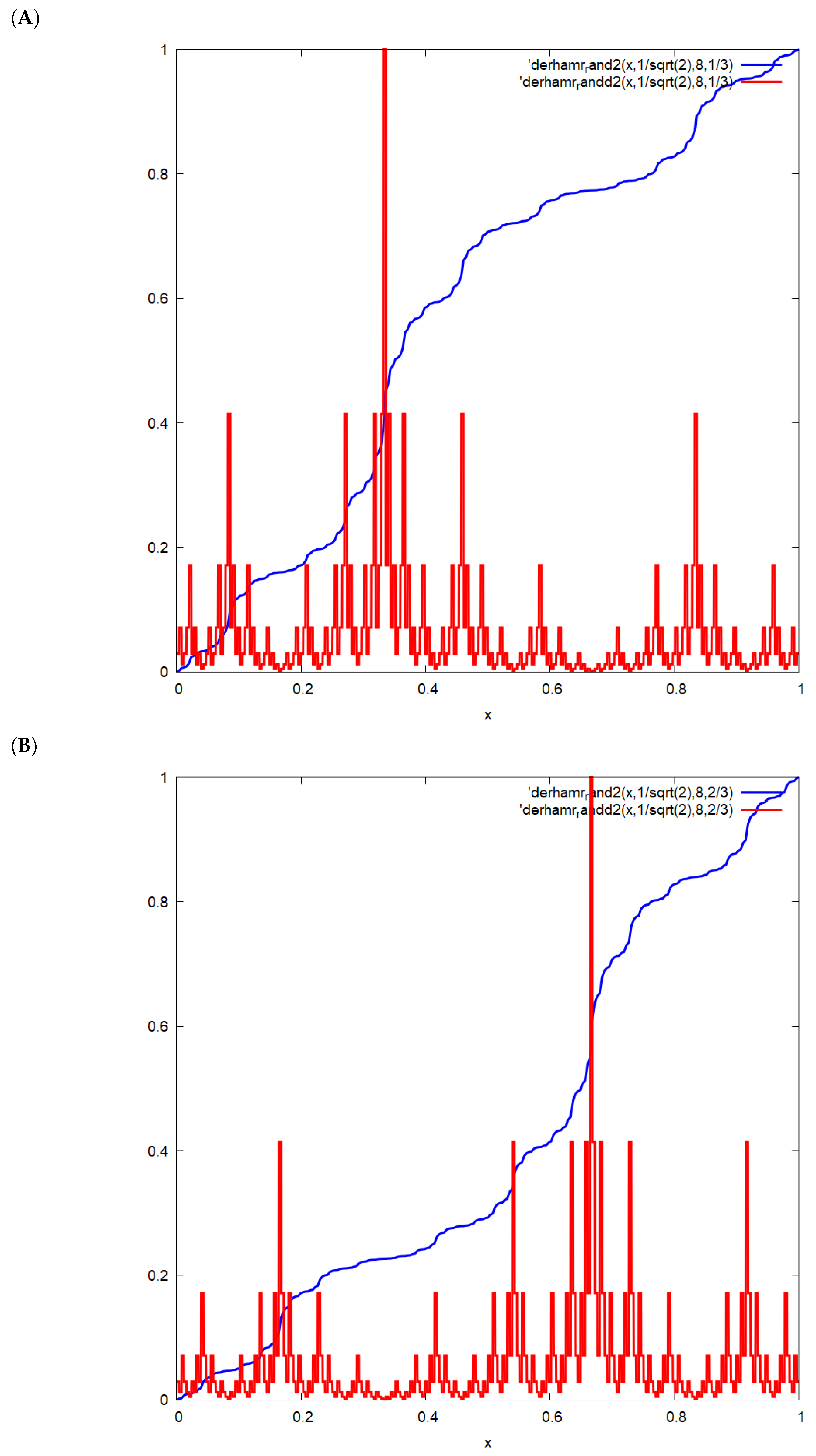
Plotting of the graph of the fractional velocity is challenging due to the fact that it does not vanish only on a null set in any given interval. Therefore, one could only plot the covering graph approximating the fractional velocity at certain iteration order. This can be done by defining recursively an IFS that in limit converges point-wise to the fractional velocity of the given singular function.

The construction of the Neidinger function can be generalized using the Bernoulli map. The result is another singular function, which we can call tentatively De Rham-Bernoulli function. The construction can be carried out as follows.

Example 6 

(De Rham-Bernoulli singular function). Suppose that $\xi \in (0,1)$. Starting from $\xi \left[0\right]:=\xi$ define $\xi \left[n\right]:=2\xi [n-1]-z[n-1]$, where $z\left[k\right]:=\lfloor 2\xi \left[k\right]\rfloor$ evaluates to either 0 or 1. Define the auxiliary function

$$b\left(\xi \right):=z(1-a)+(1-z)a$$

where z is computed as above.

Finally, starting from $M_0(x,a,\xi )=x$ define the IFS

$$M_n(x,a,\xi \left[n\right]):=\left\{\begin{array}{cc}b\left(\xi \left[n\right]\right)M_{n-1}(2x,a,\xi [n-1]),\hfill & 0\le x<{\displaystyle \frac{1}{2}}\hfill \\ (1-b\left(\xi \left[n\right]\right))M_{n-1}(2x-1,a,\xi [n-1])+b\left(\xi \left[n\right]\right),\hfill & {\displaystyle \frac{1}{2}}\le x\le 1\hfill \end{array}\right.$$

Then

$$M_{\xi }(x,a):=\underset{n\to \infty }{lim}{M}_n(x,a,\xi \left[n\right])$$

Observe that the limit exists since $b\left(\xi \right)<1$. Indeed, suppose that $a<1/2$. Then

$$b\left(\xi \right)=z(1-a)+(1-z)a<1-a<1$$

By symmetry, the same estimate holds also whenever $a>1/2$. Therefore, the IFS will converge point-wise to a limit.

The fractional velocity of the above function can be computed in a similar way as above setting $a=1/2^{\beta }$. The IFS in this case is

$$A_n(x,a,\xi \left[n\right]):=\left\{\begin{array}{cc}b\left(\xi \left[n\right]\right)2^{\beta }{A}_{n-1}(2x,a,\xi [n-1]),\hfill & 0\le x<{\displaystyle \frac{1}{2}}\hfill \\ (1-b\left(\xi \left[n\right]\right))2^{\beta }{A}_{n-1}(2x-1,a,\xi [n-1]),\hfill & {\displaystyle \frac{1}{2}}\le x\le 1\hfill \end{array}\right.$$

starting from $A_0(x,a,\xi \left[0\right])=1$. Then in order for the IFS to converge the maximal Hölder exponent is

$$\beta =-{log}_{2}b\left(\xi \right)=-{log}_{2}max(a,1-a)$$

and the IFS transforms as

$$A_n(x,a,\xi \left[n\right]):=\left\{\begin{array}{cc}{\displaystyle \frac{b\left(\xi \right[n\left]\right)}{max(a,1-a)}}{A}_{n-1}(2x,a,\xi [n-1]),\hfill & 0\le x<{\displaystyle \frac{1}{2}}\hfill \\ {\displaystyle \frac{1-b\left(\xi \right[n\left]\right)}{max(a,1-a)}}{A}_{n-1}(2x-1,a,\xi [n-1]),\hfill & {\displaystyle \frac{1}{2}}\le x\le 1\hfill \end{array}\right.$$

Note that the form of the IFS is identical to the one in the previous example. Finally,

$${\upsilon }_{+}^{\beta }M(x,a,\xi )=\underset{n\to \infty }{lim}{A}_n(x,a,\xi \left[n\right])$$

A plot of the Neidinger-Bernoulli function and its fractional variation at iteration level $n=8$ is presented in Figure 1.

6.3. Modular Derivatives on Banach Spaces

Theorem 3 formulated above can be established also in a different, more-general way. It can be used for the characterization of the modular derivatives in more general spaces. To this end we use the topological definition of limit.

Recall the definition of the directional derivatives:

Definition 24 

(Gâteaux or directional derivative). Let X and Y be Banach spaces and let $f:X\to Y$ be a function between them; f is said to be Gâteaux differentiable if there exists an operator $T_x:X\to Y$, such that $\forall v\in X$,

$$\underset{h\to 0}{lim}{\displaystyle \frac{f(x+hv)-f\left(x\right)-h{T}_x\left(v\right)}{h}}={\displaystyle \frac{d}{dh}}f(x+hv){|}_{h=0}-T_x\left(v\right)=0$$

The operator $T_x\equiv \mathbf{D}f\left(x\right)$ is called the Gâteaux derivative of f at x.

To this end, we replace $ϵ$ by the scalar-valued modulus function $g\left(ϵ\right)$. The definition of a modular function at point 3 is modified as follows:

$$|f(x+ϵv)-f\left(x\right)|\le K{g}_x\left(ϵ\right),\left|v\right|=1$$

This allows for translating the definition of g-derivatives into directional derivatives in more general spaces.

Definition 25 

(modular Gâteaux derivative). Let X and Y be two Banach spaces and $f:X\to Y$ be a function between them. Then f is Gâteaux differentiable with respect to the modulus g if there exists an operator $T_x:X\to Y$, such that $\forall v\in X$,

$$\underset{ϵ\to 0}{lim}{\displaystyle \frac{f(x+ϵv)-f\left(x\right)-g\left(ϵ\right)T_x\left(v\right)}{g\left(ϵ\right)}}=0$$

We write

$${\displaystyle \frac{d}{dg\left(ϵ\right)}}f(x+ϵv){|}_{ϵ=0}=T_x\left(v\right)$$

The operator $T_x\equiv {\mathbf{D}}_{g}f\left(x\right)$ is called the g-Gâteaux derivative of f at x in the direction v.

Theorem 4 

(Topological continuity of g- Gâteaux derivatives). Suppose that S is dense in ${\chi }_g\left(f\right)$. Then under the topology ${\mathcal{T}}_{\mathcal{Q}}$ the images ${\mathbf{D}}_{g}f\left(x\right)$ are continuous on S.

Proof. 

Suppose that the closure operator is $\mathcal{Q}$. Denote the auxiliary variation operator by

$${\upsilon }_g^{ϵ\pm }\left[f\right]\left(x\right):={\displaystyle \frac{f(x+ϵv)-f\left(x\right)}{g\left(ϵ\right)}}$$

Observe that for the limit operation $\underset{x\to a}{lim}f\left(x\right)\subseteq \mathbf{cl}f\left[A\right]\setminus f{\left[A\right]}^{\circ }=\partial f\left[A\right]$ for $x,a\in A$. Hence, if the limit exists it is continuous by Theorem A2. Then we specialize the argument to the right (resp. left for the minus sign ) $ϵ$-neighborhood of 0 and write ${\lim }_{ϵ}$ for the one-sided limiting operation. Finally, observe that ${\mathbf{D}}_{g}f\left(x\right)={\lim }_{ϵ}\circ {\upsilon }_g^{ϵ\pm }\left[f\right]\left(x\right)$ is a composition of two topologically continuous maps and hence it is continuous. □

7. Discussion

The contributions of the present work can be discussed in several directions. On the first place, Theorem 1 generalizes the result stated in [23], which in the previous case was proven only for the real line.

On the second place, Theorem 3 resolves an apparent contradiction uncovered in the early literature on local fractional calculus. To illustrate the issue and its resolution consider the Cantor function that grows on a subset ${\chi }_{\alpha }\subseteq C$, which is dense in the Cantor set C. For any $s\in {\chi }_{\alpha }$ the fractional velocity of order $\alpha =log2/log3$ is constant on ${\chi }_{\alpha }$ and moreover ${\upsilon }_{ϵ+}^{\alpha }\left[F\right]\left(s\right)$ = ${\upsilon }_{+}^{\alpha }F\left(s\right)$ =1. Therefore, we can meaningfully discuss the local fractional differential equation

$${\upsilon }_{+}^{\alpha }F\left(s\right){|}_{s\in {\chi }_g}=1$$

which, otherwise, under the usual topology of the real line, will have no solutions as proved in [17,33].

On the third place, the present work exhibits a formal methodology for computation of fractional velocities on a perfect set S, which can be summarized as follows. Identify a functional equation of the function of interest. Formally g-differentiate the equation and introduce an appropriate IFS. Establish the convergence conditions on S. This fixes the value of the maximal Hölder exponent for which the IFS converges.

In conclusion, presented topological approach enables the study of both local and non-local derivative operators within a unified framework.

References

- Uhlenbeck, G.E.; Ornstein, L.S. On the Theory of the Brownian Motion. Physical Review 1930, 36, 823–841. [CrossRef]
- Nottale, L.; Lehner, T. Turbulence and scale relativity. Physics of Fluids 2019, 31. [CrossRef]
- Feynman, R.P. Space-Time Approach to Non-Relativistic Quantum Mechanics. Rev. Mod. Phys. 1948, 20, 367–387. [CrossRef]
- Nottale, L. Scale Relativity and Fractal Space-Time: Theory and Applications. Found. Sci. 2010, 15, 101–152. [CrossRef]
- Konopelchenko, B.G.; Ortenzi, G. Homogeneous Euler equation: Blow-ups, gradient catastrophes and singularity of mappings. J. Phys. A: Math. Theor. 2021, 55, 035203. [CrossRef]
- Barnsley, M. Fractals everywhere; Academic Press Professional, 1993; p. 531.
- Dovgoshey, O.; Martio, O.; Ryazanov, V.; Vuorinen, M. The Cantor function. Exposition. Math. 2006, 24, 1–37. [CrossRef]
- Prodanov, D. Characterization of the Local Growth of Two Cantor-Type Functions. Fractal and Fractional 2019, 3, 45. [CrossRef]
- Minkowski, H. Zur Geometrie der Zahlen. In Gesammelte Abhandlungen; Teubner, 1911; Vol. 2, pp. 50–51.
- Salem, R. On some singular monotonic functions which are strictly increasing. Transactions of the American Mathematical Society 1943, 53, 427–439. [CrossRef]
- Ryabinin, A.A.; Bystritskii, V.D.; Ilichev, V.A. Singular Strictly Monotone Functions. Mathematical Notes 2004, 76, 407–419. [CrossRef]
- Carpinteri, A.; Mainardi, F., Eds. Fractals and Fractional Calculus in Continuum Mechanics; Springer Vienna, 1997. [CrossRef]
- Milanov, S.; Petrova-Deneva, A.; Angelov, A.; Shopolov, N. Higher mathematics, part II; Technika, 1977.
- Parvate, A.; Gangal, A. Calculus on fractal subsets of real line : I Formulation. Fractals 2009, 17, 53–81. [CrossRef]
- Parvate, A.; Satin, S.; Gangal, A.D. Calculus on Fractal Curves in Rn. Fractals 2011, 19, 15–27. [CrossRef]
- Cherbit, G., Fractals, Non-integral dimensions and applications. In Fractals, dimension non entière et applications; John Wiley & Sons: Paris, 1991; chapter Local dimension, momentum and trajectories, pp. 231– 238.
- Prodanov, D. Conditions for continuity of fractional velocity and existence of fractional Taylor expansions. Chaos, Solitons & Fractals 2017, 102, 236–244. [CrossRef]
- Chen, Y.; Yan, Y.; Zhang, K. On the local fractional derivative. J Math Anal Appl 2010, pp. 17 – 33. [CrossRef]
- Prodanov, D. Fractional Velocity as a Tool for the Study of Non-Linear Problems. Fractal and Fractional 2018, 2, 4. [CrossRef]
- Hristov, J. The Fading Memory Formalism with Mittag-Leffler-Type Kernels as A Generator of Non-Local Operators. Applied Sciences 2023, 13, 3065. [CrossRef]
- Kolwankar, K.; Gangal, A. Hölder exponents of irregular signals and local fractional derivatives. Pramana J. Phys 1997, 1, 49 – 68.
- Golmankhaneh, A.K.; Fernandez, A.; Golmankhaneh, A.; Baleanu, D. Diffusion on Middle-ξ Cantor Sets. Entropy 2018, 20, 504. [CrossRef]
- Prodanov, D. Local generalizations of the derivatives on the real line. Commun. Nonlinear Sci. Numer. Simul. 2021, 96, 105576. [CrossRef]
- Kuratowski, K. Topology Volume I; Academic Press: New York, 1966.
- Prodanov, D. Generalized Differentiability of Continuous Functions. Fractal and Fractional 2020, 4, 56. [CrossRef]
- Angenent, S.B.; Fila, M. Interior gradient blow-up in a semilinear parabolic equation. Differential Integral Equations 1996, 9. [CrossRef]
- Konopelchenko, B.G.; Ortenzi, G. On universality of homogeneous Euler equation. J. Phys. A: Math. Theor. 2021, 54, 205701. [CrossRef]
- Kwaśnicki, M. Ten Equivalent Definitions of the Fractional Laplace Operator. Fract. Calc. Appl. Anal. 2017, 20, 7–51. [CrossRef]
- Šilhavý, M. Fractional vector analysis based on invariance requirements (critique of coordinate approaches). Continuum Mech. Thermodyn. 2019, 32, 207–228. [CrossRef]
- Takács, L. An Increasing Continuous Singular Function. Amer. Math. Monthly 1978, 85, 35–37. [CrossRef]
- de Rham, G. Sur quelques courbes definies par des equations fonctionnelles. Univ. e Politec. Torino. Rend. Sem. Mat. 1957, 16, 101 – 113.
- Neidinger, R. A Fair-Bold Gambling Function Is Simply Singular. The American Mathematical Monthly 2016, 123, 3. [CrossRef]
- Adda, F.B.; Cresson, J. Fractional differential equations and the Schrödinger equation. App. Math. Comp. 2005, 161, 324 – 345.
- Wikibooks. General Topology — Wikibooks, The Free Textbook Project, 2018. [Online; accessed 12-April-2019].