

Submitted:
02 December 2024
Posted:
03 December 2024
You are already at the latest version
Abstract
KThe article discusses the application of spatial statistical models in Remote Sensing (RS), which appears to be an important source of spatial data at multiple scales. However, to derive the maximum information, it is necessary to apply appropriate techniques of spatial statistics by de-fining a spatial statistical model. A crucial problem facing us is the fusion of multi-source spatial data of different nature and characteristics. One of these properties is the support of measurement, which unfortunately is little considered in RS. Therefore, a multivariate geostatistical approach is proposed that can fuse data of different types, including soil sample, hyperspectral, multispectral UAV and satellite data, considering the various supports and their impacts on prediction and its uncertainty. The method is applied to soil data after filtering UAV images of an olive grove. The fusion of soil sample data with hyperspectral data measured in the laboratory, UAV and satellite data (Planet and Sentinel 2) improved the prediction accuracy of the soil properties compared with univariate prediction. It is hopeful that advanced spatial statistical techniques will be increasingly applied in RS in the future.
Keywords:
hyperspectral data
; PLSR
; change of support
; data fusion
; convolution
; deconvolution
1. Introduction
The use of remote sensing in mapping and assessment of soil resources is constantly increasing, as is the possibility of achieving ever greater spatial resolution. There is a rich literature on the applications of remote sensing in soil ranging from general assessment of soil resources and its main properties for different purposes [1,2,3,4,5]. Interest covers the application of remote sensing in agriculture [6] and especially in precision agriculture [6,7].
The application of remote sensing requires the use of explicit spatial statistical techniques whose appropriateness needs to be proven even though they are widely used, and any shortcomings of them might require new spatial statistical modelling approaches. Geostatistics [8,9] is a suitable approach to spatial modelling remote sensing data and its use is almost missing although the link between remote sensing and geostatistical methods was established in the late 1980s [10,11,12] to quantify image spatial structure [13,14,15], integrating spatial statistics and remote sensing [12], image classification [16]. Remote Sensing is a great source of spatial (and space–time) environmental data and geostatistical methods can be to right approach to many issues arising from their analysis.
The set of measurements of reflectance obtained from a scene is associated with a spatial position in the scene and, therefore, as a regionalized variable function of spatial position and neighboring points in the scene are consequently more similar spectrally than distant points [17,18]. That is called spatial autocorrelation, and it disappears with distance. The mean distance at which this spatial autocorrelation disappears is related to the size, spacing, and shape of the objects in the scene [17,18]. The spatial structure resulting also depends on the spatial resolution of the sensor with respect to the objects imaged. Therefore, to use data from different remote sensors, it is necessary to consider three basic concepts related to a remote sensing image: support, spatial resolution and pixel [19,20]. The support is an important geostatistical concept representing the space on which a measurement or observation is made, and it is characterized by geometrical shape, size, and spatial orientation [19,21]. It should not be confused with spatial resolution [22] ,which represents the average sampling distance in sparse sampling, whereas support is the size of the grid mesh or pixel [20].
Using remote sensing data from different satellites or sources it is required to define a data fusion of heterogeneous spatial data for prediction which considers the different supports. The support of measurement in RS is commonly represented by a 2D Gaussian function (or similar function) referred to as the ‘point spread function’ (PSF), with its tails extending far beyond the limits of a pixel [23]. Little spatial statistics research in remote sensing has been devoted to the impact of support and PSF shape on the prediction and its uncertainty. It is worth underlining that the main target of spatial statistics in RS is to extract information from remotely sensed data. Information can be defined as the difference between data, and therefore in a single waveband remotely sensed image information consists in the differences between neighboring pixels [24]. This concept is sufficiently general [23] and allows the variance of a Gaussian data distribution to be used as a diagnostic tool because it describes what is expected on average. In the case of spatial data, its extension to the concept of a spatial covariance function is particularly useful. It is possible to calculate the empirical spatial covariance and to fit a model to it by using an appropriate method of inference. Common permissible (authorized) functions include the Matérn family of models, such as the popular exponential covariance model. The exponential model has two parameters, the so-called sill variance and range (or practical range). To a certain extent, the sill variance of the exponential model can be thought of as the spatial equivalent of the sample variance. The range on the other hand has no equivalent in the data distribution in traditional statistics. However, the range parameter is very useful because it tells us a lot about the potential information content of an image. The range in fact informs about the scale(s) of spatial variation present in the image [19,25,26,27,28,29,30] and represents the upper limit of spatial correlation between observations. Also, the shape of the spatial covariance function is quite informative. For example, the exponential model, which is asymptotic towards the sill variance, can be assumed representing a set of scales of variation, each with its own information-to-redundancy ratio. Yet in recent times there has been a lack of interest in RS in dealing with spatial statistical functions and in particular spatial covariance functions, neglecting all the potential information about the nature of the variable of interest that they can provide us with geostatistics [24].
Remote sensing images are essentially tables of data commonly represented by digital numbers. However, when the main interest is extracting information from these data, it is essential to define statistical models that can characterize the spatial variation and thus predict a variable of interest at points where sampling or observation has not been done. Indeed, various techniques exist to do this, such as geostatistics and its recent developments in multi-point geostatistics [31,32], spatially explicit regression models that introduce spatial dependence between pixels [33] and more recently Machine Learning techniques [34,35]. This paper is mostly focused on the application of geostatistics to RS data.
Geostatistical model can in fact be used for (i) handling missing data (e.g., generated by the presence of clouds or cloud shadow [36,37], or by a sensor's operation failures [38]; (ii) upscaling from a set of pixels to a bigger (regular or irregular) block [39]; (iii) downscaling from a coarse pixel to a finer spatial resolution [40,41] ; and (iv) fusion of images of a certain spatial resolution with other images of a different spatial resolution [42]. Both upscaling and downscaling involve the problem of change of support which initially was addressed to eliminate the strictures of the pixel in RS. Pixel is considered as the average reflectance of light from a limited support, therefore decomposing the original support into a set of finer supports is indeed a fairly common problem, widely reported but not easy. This can be done if additional information is available in a multivariate approach, which means fusing multi-source data with different support. Multivariate geostatistics provides a way to solve the downscaling problem in RS, which is particularly crucial in the presence of mixed pixels and in the application of site-specific management in agriculture. A key concept in geostatistical analysis is the spatial covariance function, or its related function, the variogram, which characterizes the spatial variation and parameterizes a random function (RF). Under the condition of second-order stationarity, remotely sensed images can be treated as a realization from a RF and then it is possible to apply geostatistical techniques in fusing them with different kinds of data considering their respective supports. Indeed, there is currently a scarcity of attempts in RS that apply downscaling or upscaling considering change of support with its implications on the variance of estimation or better on the spatial dependence function [43].
The choice of spatial resolution is an extremely crucial problem in RS, because the pixel size could be too large relative to the scales of variation of the process which remains the researcher’s main interest rather than the image itself, i.e. an understanding of reality with its mechanisms and functions.
Geostatistics offers the possibility to fit mathematical-statistical models defined on punctual support to the data on finite support such that other mappings can be generated readily (e.g., to coarser support, to a finer support or to a support with complex geometry such as Management Zones (MZ) in Precision Agriculture). It is quite important, because one of the most significant challenges in environmental data science today is the inability to allow datasets, that were obtained with different supports and with other measurement characteristics, to speak to each other [44]. Interoperability among different data sets requires that data on one support can be changed to data on another support reciprocally. This demand can be addressed by an appropriate multi-source data fusion approach although, unfortunately, such a vision is not common, especially in RS. Nevertheless, it is a crucial issue that needs to be addressed because environmental data comes in a wide variety of shapes and sizes (property definitions, sampling frameworks, measurement characteristics, error characteristics). Dealing jointly with this multiplicity of heterogeneous data properly and drawing as much information as possible is not a trivial problem and should appeal to spatial statisticians.
Moreover, geostatistical RF characterizations can be helpful in revealing the scales of spatial variation in spatial data and the potential information content or conversely, the redundancy in data. They can also provide some insights into the data which can have different uses, such as stating whether a particular sampling or method is appropriate for a task: using the right model for the right task by considering one's own purposes carefully.
The objective of this paper is to propose an approach for spatial statistical modelling in remote sensing of land cover by fusing data of different types. Agricultural land use composed of different land covers as soil and trees arranged spatial patterns was considered. The results of this study may provide useful insights and foster discussion on conceptually important topics in relation to the development and application of spatial statistics in RS.
2. Materials and Methods
2.1. Study Area and Soil Data
The study area (Figure 1) is an olive grove (’Ogliarola Salentina’ cultivar) located in south-eastern Italy (Brindisi, 40°31′10.57′′ N; 17°39′42.86′′ E). The field is flat and gravel free and soil is classified as Calcic Haploxeralf [45]. “Calcic” regards a calcic horizon with its upper boundary within 1 m of the mineral soil surface, and “Haploxeralf” involves a loamy granulometry and a relatively thin argillic or kandic horizon.
Composite topsoil samples (0–0.20 m) were collected in July 2019 at 61 locations around each olive trees. Three soil samples were collected around the trees (at about 1 m) and were mixed. More details on the study area can be found in Belmonte et al. [46].
Soil samples were analyzed in the laboratory for different properties, but here only textural fractions were included in the study. The different soil textural fractions (%) were classified according to the particle size limits used in the USDA scheme [47]: total sand (2.0-0.05 mm), silt (0.05–0.002 mm), and clay (<0.002 mm). Clay, silt and coarse sand (2.0–0.2 mm) were determined by pipette method [48]. Total sand represents the sum of coarse and fine sand (0.2-0.05 mm); the latter was calculated as the complement to 100 of the sum of the measured soil particles fractions.
2.2. Hyperspectral Analysis
VIS-NIR-SWIR reflectance of topsoil (0–0.20 m) was measured in laboratory on a fraction of the soil samples collected for granulometry analysis with an ASD FieldSpec IV spectroradiometer (Analytical Spectral Devices Inc., Boulder, Colorado, USA) over a spectral range of 350–2500 nm [49]. The spectra were averaged over 10 nm so reducing the number of wavelengths from 2151 to 215 to smooth them and avoid the risk of over-fitting [50].
The following spectral pre-processing methods were carried out to reduce the multiplicative and additive effects, preserving the useful information for prediction models [51]: 1) multiple scatter correction (MSC) and standard normal variate (SNV); 2) smoothing/denoising with Savitzky–Golay polynomials (SG). Multiplicative scatter correction (MSC) removes additive and multiplicative components [51,52], mostly due to scatter effect so reducing the number of components needed in the calibration model and improving the linearity [51]. The Standard Normal Variate (SNV) method carries out a normalization of the spectra that consists in subtracting each spectrum by its own mean and dividing it by its own standard deviation [52]. After SNV, each spectrum will have a mean of 0 and a standard deviation of 1: the result is like that of MSC. SNV is frequently used to compensate for changes in surface roughness of the material [53].
Savitzky–Golay (SG) algorithm [54] reduces the random noise of the measurements. For a given spectrum measured at N points and a filter of width w, it calculates a polynomial fit of any order in each filter window as the filter is moved across the signal. The size of the filter consists of (2n + 1) points, where n is the half-width of the smoothing window (w). The filter calculation is complete when the filter window moves the signal one-at-a-time. A window size (w) of 11 (w = 2n+ 1) and polynomial order of two were applied [55].
Spectral data transformation and pre-processing were performed with ParLeS software [56].
Different combinations of the pre-processing methods were compared to the use of raw data of reflectance by assessing the performance of prediction models [57].
2.3. Prediction Models
To estimate soil granulometric fractions, Partial Least Squares Regression (PLSR) [58] was applied. PLSR is based on decomposition of two sets of variables: the matrix X of predictors (matrix n x NX, where n is the number of observations (61) and NX is the number of spectral data at different wavelengths (215)), and the vector Y of the response variable (sand or clay or silt). PLSR selects successive orthogonal factors (or latent variables) that maximize the covariance between predictors (X, reflectance) and response variable (Y, sand or clay or silt) and explains most of the shared variation. For more details on PLSR method. Leave one out cross validation was performed to determine the number of latent variables that minimized the predicted residual sum of squares (PRESS). Each calibration set is created by taking all the samples except one, the validation set being the sample left out. The performance of PLSR prediction model was evaluated by means of three statistics: (1) the coefficient of determination R2 of the regression: observation vs. prediction; (2) root mean square error of prediction (RMSEP), and 3) the ratio of performance to interquartile distance (RPIQ) [59] defined as follows:
where:
yi are the observed values, yi’ the predicted values, and n is the number of samples with i=1, 2,…, n.
IQ is the difference between the third and first quartiles of y:
RMSEP has the same unit of measurement as the dependent variable therefore RPIQ is unitless and an inverse measure of error related to population spread, the greater than 1.5-2 the better. R2 measures the precision of each model and the higher the value the better the fit. After cross-validation, analysis of residuals was performed with Shapiro-Wilk and Kolmogorov-Smirnov tests, to evaluate if the distribution was normal. When the probability level for both statistics was greater than 0.10, the distribution was assumed normal [55].
To identify the best wavelength ranges for prediction, the analysis was performed both on the full range and on specific ranges by analyzing 100 nm intervals at a time. The ranges, causing a model with the highest R2, were chosen. Thus, for clay were selected the wavelengths between 360-440 nm and 1560-2500 nm, while for sand and silt 450-1350, 1430-1550 and 2060-2400 nm.
A total of 108 models were carried out, based on: 1) two types of data: reflectance and absorbance; 2) 9 combinations of the pre-processing methods on reflectance and absorbance data; 3) 3 granulometric fractions, clay, sand and silt; 4) 2 wavelength ranges: full (350-2500 nm) range and selected ranges as described above.
2.4. Remote Sensing Products
Reflectance unmanned aerial vehicle (UAV) acquisition data
The high spatial UAV image was acquired on July 2019 with a DJI Mavic Pro drone whose custom payload carried a multispectral sensor (Parrot Sequoia) that captures data (16 Megapixel) with four bands (see Table 1) at 70 m height and with a theoretical resulting Ground Sampling Distance (GSD) of 0.07 m/pixel. The mission flight plan is managed by the Mission Planner software which ensures 80% front and side overlap of the frames. The reconstruction of the scene is performed by version 4.4.12 of Pix4d Mapper Pro software by applying Structure from Motion (SfM) [60] techniques on a total of 1152 images acquired (288 frames for each multispectral band). A final orthophoto image for each band was generated from a quoted point cloud.
Reflectance Planet acquisition data
In recent years new commercial satellite platforms, such as PlanetScope, have become available. PlanetScope is operated by Planet Labs [61]. This platform is a CubeSats constellation that consists of over 180 satellites deployed in sun synchronous orbit with a daily revisit time, which offers more opportunities for cloud-free images. The first Planet satellites were launched in 2015. The first generation satellites have an optical multispectral sensor with four spectral bands at red, green, blue, and near-infrared wavelengths, with a spatial resolution of 3.7 m at nadir; while the new generation of PlanetScope satellites has the potential to produce imagery with eight spectral bands.
In this study the reflectance of PS2 product Plane, orthophoto image, with four bands (see Table 1) was used. This product is into unit16 data type, to represent the data into range [0, 1] it is necessary to divide by 10000, as specified into metadata.
The Planet image was downloaded from Planet website [62].
Reflectance Sentinel 2 acquisition data
The Sentinel 2 image was downloaded from Copernicus Space Data Ecosystem (CDSE) Portal [63]. The S2-MSI satellite data, as surface reflectance product, were used for this work. This satellite was launched in 2015 by the European Space Agency (ESA) with a variable spatial resolution from 10 to 60 m and thirteen spectral bands. In detail we worked with Level-2A data that provides atmospherically corrected bottom of the atmosphere reflectance images.
In this work all UAV bands, all Planet bands and only two Sentinel 2 bands (11 and 12 one), see Table 1, were used as auxiliary variables in the process of soil property prediction. All the images have been chosen so that their acquisition date was as close as possible to the samples date.
2.4.1. Filtering of Soil Data from Remote Sensing Product
- −
- UAV and Planet data
The processing focuses on retrieval soil information involved supervised classification to select thematic information. The process was using the following principal steps present in the commercial ENVI (ENvironment for Visualizing Images) 5.1 software (Harris Geospatial):
- −
- Training Samples
To identify thematic information, the set of ground cover types (i.e., information classes) into which the image would be segmented was first determined. Prototype pixels, or training samples, were then assigned to these selected classes. At the beginning, for this study, three classes were chosen based on different but sufficiently homogeneous regions of the same image: soil, canopy, and shadow. To account for class variability and minimize the influence of transition areas where mixed pixels may occur [64], enough training pixels (at least 150 pixels per class) were selected. This ensured a representative sample of each class.
- −
- Maximum likelihood
The training data were applied to estimate the parameters for the classifier algorithm. The decision rule applied was the maximum likelihood method, utilizing a Gaussian model. This process resulted in the generation of a thematic map, with the desired classes clearly delineated.
- −
- Morphological filter
To keep intact the geometric structure of image objects, a morphological filter based on the closing operator [65] was applied. This operator modifies the geometric features of the signal by removing small holes within polygons. The morphological convolution is performed on the signal using a structuring element, which is a set of simpler shapes and sizes [66].
- −
- Combine classes
This step is used to build a binary image merging two classes (canopy and shadow) into one class labeled ‘soil’, identified with 1 respect to class ‘not-soil’, identified with 0.
- −
- Conversion raster to vector
The binary images on each UAV and Planet satellite band [49] were converted from a labelled raster image into vector data format (such as ESRI Shapefile format), employing the tool (r.tovector) of the GRASS (Geographic Resources Analysis Support System) module integrated in the open-source software: QGIS (Quantum Geographic Information System) version 3.38.0 – Grenoble.
- −
- Soil information
To retrieval soil information the ‘raster extraction’ tool available in QGIS was applied. By it each raster image is clipped by mask layer formerly created into shapefile format.
For Sentinel-2 bands 11 and 12, soil retrieval is performed exclusively using a geostatistical method, as described in Section 3.2, due to their too coarse spatial resolution (20 m).
2.5. Geostatistical Multi-Source Data Fusion
Spatial data conversion between different spatial scales is a common challenge in environmental applications because of spatial mismatch between different data sources, such as various types of observation sensors in Remote and proximal sensing and /or sample collection methods. One of spatial support include the pixel size in satellite imagery. Spatial support is a very important concept in geostatistics because it determines the scale at which spatial variability of input variables can be analyzed and the one of the predictions.
Change of spatial support refers to changing from one type of spatial support to another during the spatial prediction. Using the terminology by [67], upscaling consists in aggregating point data into an area and downscaling in disaggregating an area data into points.
Accurate downscaled information is crucial for making decisions in precision agriculture or environmental management. Geostatistical spatial scaling for remote sensing downscaling was used by [40]. In the case of co-registered multivariate satellite sensor images, [68] proposed area-to-point downscaling cokriging, where the pixel size to be predicted is smaller than the one of the input images.
A practical problem of interest in remote sensing is to transform a coarse spatial resolution image into another fine spatial resolution image by introducing spatial ‘detail’ but in a way that is coherent with the spectral information of the original image. A particular solution is provided by area-to-point kriging [69], but in most cases more than one experimental variable may be represented on different supports and the support of the variable to be predicted may not be a point. This is often the case in remote sensing, where a satellite sensor may provide different images for several spectral wavebands with potentially different spatial resolutions (pixel sizes). In such cases, a problem of digital image analysis is to combine the images to increase the spatial resolution (i.e. decrease the pixel size) of the coarser spatial resolution images while preserving their spectral content. The objective may be twofold: improving the visual aspect of the image and facilitating image interpretation for better e.g. soil characterization. However, most of the existing algorithms for image fusion are aimed at obtaining a visually pleasant image but do not consider the spatial autocorrelation of the waveband and then its spatial structure either at coarse or fine resolution. Moreover, in order to jointly analyze (fuse) multi-source data, both sample and grid data such as RS images of different resolution , geostatistics uses a multivariate interpolator (cokriging) which has several advantages compared with traditional approaches in RS, already underlined by [70]: 1) provides a prediction which is unbiased and minimizes the prediction variance; 2) explicitly takes into account the support (pixel size in RS) of each variable via its variogram; 3) takes into account the correlation structure via the set of direct and cross variograms; 4) can explicitly take into account the point spread function (PSF) of the satellite sensor. PSF makes it possible to describe the response of an optically focused (image) system to a point source or object; and 5) provides an estimate of the uncertainty of the prediction.
To be able to use point cokriging applied to the entire multivariate data set, including the sample soil variables, satellite images (Planet and Sentinel2) and UAV images, it was necessary to reduce in advance all variables to the same point or reference support.
Assuming as the reference (point) support that of the soil samples (i.e. a 1m x 1m block), the satellite images were deconvolved to the same block through deconvolution by kriging, while the UAV images were convolved to the same block through block cokriging.
Below the whole approach used to fuse the multi-source data of our study is illustrated and the techniques used were briefly described. The interested reader may refer to the numerous bibliographical references given for further details.
2.5.1. Deconvolution of Images by Kriging
In image analysis using satellite or UAV images the available data are not on a point support but are convoluted by a weighting function on an extended area (pixel). This function depends on the underlying physical process and the characteristics of the sensor, and can be established from theoretical considerations, or can be measured with appropriate experiments [71]. Various approaches enable images to be deconvoluted. All these approaches are very common in the image analysis literature [72]. Deconvolution of images is generally treated by Fourier transformation. However, this approach is known to be not applicable when considering convoluted data with noise or when a regular grid of data is not available and therefore missing data have to be interpolated. It is for this reason that in this work another approach was used based on the process of estimating point data by deconvoluting kriging [71].
An image in Rn Y(x) at the finer pixel x can be modified through a convolution by a weighting function , which is normalized, so that its integral over spatial coordinates is equal to 1, and . Experimentally, the observed data Z at coarser pixels xα are given by:
Therefore, knowing the weighting function , the problem is to estimate the image at each pixel x from the data known at coarser pixels . This can be done by estimation with kriging. The weighing or convolution functions depend on physical conditions, however the most common are: uniform, exponential, gaussian and sinc functions [71]. This approach has been developed in the frame of geostatistics [73] and considers information on the spatial structure of the underlying phenomena. It essentially consists in the estimation of the unknown data by a local linear regression. Applications to RS image analysis have already been proposed [68,74] but they are not very common, especially in recent years when Machine Learning techniques are preferred. Here we consider the common case of a single datum per pixel x, such as the recorded reflectance at a given wavelength. The variables and are assumed to have the same mean and to be realizations of an intrinsic random function, whose increments are assumed as a second order stationary random function (Webster and Oliver, 2006). In geostatistics variogram is the cornerstone of the prediction, which for the random function Z is defined as follows:
where E is mathematical expectation. To estimate the underlying variable from the observed variable , an estimator , i.e. a linear combination of data in a neighborhood of x (pixels ), was used:
The weights in equation () are the unique solution of the linear kriging system, obtained from unbiases and minimal error variance conditions for the estimate:
where is a cross-variogram:
and the variance of the estimate is given by , where is Lagrange multiplier.
The practical implementation of deconvolution by kriging requires one to solve the cokriging system (Equation 6) after performing a so-called structural analysis to estimate the underlying variogram . The procedure consists of different steps:
- 1.
- Calculation of the experimental variogram from data Z. This variogram should show a nugget effect in the presence of noise, followed by very regular behavior for small distances h, due to the convolution function ;
- 2.
- Choice of a variogram model for , possibly including different scales. Theoretical models are inferred from a priori knowledge of the structure and from the behavior of the experimental variogram and setting of supports of the variables and
- 3.
- Calculation (mostly by numerical interpolation) of a theoretical model of from , and .It is worth pointing out that if the knowledge of is necessary, otherwise no correct deconvolution can be expected;
- 4.
- Comparison between experimental and the model variogram. If necessary, perform correction of the model and repeat steps 2-3-4;
- 5.
- Choice of the optimal neighborhood and numerical solution of the cokriging system (Equation 6);
- 6.
- Restoration of the image from the system of weights and calculation of the quality of the deconvolution. This procedure is implemented in the software package ISATIS Release 18.5 (www.geovariances.com) and was developed by [71].
2.5.2. Coregionalization Data Set
The multivariate data set of the case study included both sample variables (point vectorial variables) and gridded areal variables (raster variables). The target variables or variables of interest were the soil texture variables (clay, silt and sand). However, only clay and sand were subjected to the multivariate geostatistical analysis, while silt was obtained as a complement to 100 of the sum of the other two texture components. This was made necessary by the fact that not all texture components were independently measured, as above described. Therefore, the three variables were linearly dependent, thus making the resolution of the cokriging system impossible because of the singularity of the coefficient matrix. The auxiliary variables were both sample (clay and silt predictions using hyperspectral spectra) and raster (all the RS bands of UAV and Planet), while for Sentinel 2 only the R11 and R12 bands were used as they were [49].
To apply data fusion according to the techniques of multivariate geostatistics, it is necessary, after having reduced all study variables to the same support (1 m x 1 m), to construct a coregionalization data set to have enough pairs of observations to calculate cross-variograms. These calculations require using the migration procedure: move the closest pixel of the grid variables to each soil sample, if the distance does not exceed a threshold, as small as possible (1 m here, i.e. the size of one pixel), which allows obtaining sufficient observation pairs. Sixty-one was the number of observations for the multivariate coregionalization data set.
2.5.2.1. Linear Model of Coregionalization (LMC)
The multivariate spatial correlations were modelled using the linear model of coregionalization (LMC) [75], which assumes all the n variables as produced by the same independent physical processes, acting on NS different spatial scales. Therefore, the n(n + 1)/2 direct and cross-variograms (a direct variogram for each variable and a cross-variogram for the pair of variables) are modelled as a linear combination of the same series of NS basic functions of variogram :
where is the model of cross-variogram between variables Zi and Zj; the apex u indicates the spatial scale; h the lag, and the coefficients of the function , namely the partial sills of the variograms at each scale u [76]. Putting these coefficients together for each scale u, the corresponding coregionalization matrix is obtained, which can be interpreted as a variance-covariance matrix at the scale u.
2.5.2.2. Multicollocated Cokriging with Images Deconvoluted by Kriging
To fuse the sample variables with gridded variables for the final prediction of soil properties (clay and sand contents), the variant multi-collocated point cokriging was preferred rather than ordinary cokriging [77,78,79]when modelling sparse primary variables with secondary information much more finely sampled. As using all secondary exhaustive information contained within the interpolation neighborhood may lead to an intractable solution, due to too much information (big data), only the secondary data at the target location (where the estimation of the primary variable is required) and at points where the primary variable is available are employed for interpolation. This simplified version has generally produced more reliable and stable results than more known collocated cokriging, that uses only the secondary variable collocated with the position where the primary variable is sought [80].
Since the secondary datum collocated with the target position tends to screen out the influence of other secondary data placed at a larger distance, the loss of accuracy in considering the reduced neighborhood is indeed mostly negligible. However, the loss of information is well compensated for by the considerable reduction in computer time requirements.
To assess the influence of the auxiliary variables on the prediction of clay and sand content, the previous approach was compared with the univariate kriging prediction of the same variables. To perform this comparison, cross-validation [81], whereby one observation is temporally removed from the data set and re-estimated from the remaining data.
For the comparison the three statistics suggested by [82] were used:
where Z() is the estimate of soil property at site , is the observation at the same site, is the root mean squared prediction error of Y(x)). Mean error (ME) was used to assess the unbiasedness of the predictor and its optimal value should be approximately zero; Root Mean Squared Standardized Error (RMSSE) assesses the accuracy of mean squared prediction error and should be approximately 1; Root Mean Squared Error (RMSE) checks the goodness of prediction, and the approach with smaller value should be preferred because this means that predictions are closer to the observed values.
To make the comparison between the univariate and multi-source data fusion approaches more complete, the coefficient of determination (R2) between measured and estimated values and the correlation coefficient between the standardized error and the estimate (ρ) were also calculated. The latter, if the spatial model is indeed free of systematic errors, should be statistically not different from zero.
3. Results
3.1. Hyperspectral Data
Table 2 reports the results obtained with PLS analysis regarding the applied pre-treatment methods with a R2≥0.5, for the prediction of granulometric contents. All the selected models for clay and sand show a good performance with RIPQ > 2. The raw data of clay reflectance showed a model with a R2<0.5 using 'whole spectrum from 350-2500 nm (full range). Differently, when the wavelengths were selected from 360-440, 1560-2500 nm ranges, the performance improved sharply with data pretreated with SG. The first range comprises the absorbance peak of goethite (at around 420 nm), an iron oxide [83]; the second range includes the absorption peak of montmorillonite (at around 1900 nm), a component of clay, and that of kaolinite (at around 2200 nm), which is found to be strongly associated with clay [84].
The best model for sand reflectance data was obtained by considering the full range after pretreatment with SG (Table 2). A comparable R2 (0.56) occurred when using ranges between 450-1350, 1430-1550 nm and 2060-2400 nm, where reflectance tended to increase. However, in the latter case the residual distribution can be assumed normal. The above results should thus suggest that the prediction of clay is mostly affected by those wavelengths corresponding to the maximum of absorbance and then to the minimum of reflectance. Differently for sand whose prediction seems to be more affected by those wavelength intervals in which reflectance tends to increase. However, it should be emphasized that in the interval (1430-1550 nm), not included in the clay model, the absorption peak of illite, a component of clay, occurs. This result might probably be due to the chemical affinity of this clay component, consisting mainly of silicates, with sand [85]. As regards the range between 2060-2400, which is shared by the clay and sand models, an explanation for its impact on clay prediction may probably be the occurrence of kaolinite peak absorption [84], while for sand the issue merits further investigation.
For silt no models reached R2 >0.5 and the best model was obtained with the same ranges of the sand model. This probably depends on the chemical and mineralogical composition of the silt. The above results underline the importance of knowing the mineralogy of the soil before estimating the granulometric components with spectroscopy.
3.2. Geostatistical Processing
3.2.1. Deconvolution of Planet and Sentinel2 Data
The iterative approach described in Materials and Methods was implemented by fitting a nested spherical variogram model to the original areal satellite data and using a Gaussian function as a weight function according to the PSF information of the sensors on board the Planet and Sentinel 2 satellites. Table 3 shows the results of the structural analysis (variogram model determination) for each band of Planet and for bands B11 and B12 of Sentinel 2.
As can be seen from Table 3, a support ratio of 0.33 for Planet and 0.05 for Sentinel 2‘s B11 and B12 was used, roughly corresponding to the ratio of the reference pixel size (1 m) to that of Planet (3.17 m) and B11 and B12 (20 m).
This ratio is very crucial in deriving the variogram model of the deconvolved variable, as it determines the nugget ratio of the two (raw and deconvolved) variograms. Lacking direct knowledge of the deconvolved variable, this ratio is subject to great uncertainty and the estimation of the variogram model is not uniquely determined. The quality of the deconvoluted variogram model can only be estimated from a careful analysis of the deconvolved image and the possible existence of bias or artefacts with respect to the raw image. With regard to the variogram model for the Planet bands, it consists of 3 structures: a nugget, a spherical model with a short range varying between 8.48 m and 20 m, and a spherical model with a long range varying between 33.97 m and 52 m. For the B11 and B12 bands, given their close correlation, a multivariate approach was used with an estimated LMC including only one structure, that is, an exponential model with a range of 57 m. The greater simplicity of the variogram model of the Sentinel2 bands compared to those of Planet is probably due to the greater pixel coarseness. However, it should be noted that the longer-range structure is quite consistent between the two types of satellites. This leads us to think that spatial association structures of an average size of approximately 50 m do indeed exist in the study area, probably related to intrinsic variability of soil as surveyed also with different sensors [49,86].
Figure 2a shows on the left the maps of the Planet reflectance band after the filtering of the soil data because of the screen operated by the olive tree canopies; on the right side (Figure 2b) instead the corresponding whole soil images are shown at 1m resolution after applying deconvolution by kriging. Whereas for the raw B11 and B12 bands the soil maps were not retrieved due to pixel coarseness (spatial resolution 20 m).
Figure 3 instead represents the corresponding whole soil images of B11-B12 Sentinel2 bands at 1m resolution after applying deconvolution by kriging. In general, it can be said that the deconvoluted images show a high degree of coherence with each other, and no clear biases are evident, e.g. due to tree proximity, or artefacts resulting from the iterative fitting process and/or interpolation. Instead, all deconvoluted images display a sufficient degree of continuity derived from the raw images. Clearly the maps show different patterns of spatial association and distinct levels of reflectance depending on the wavelength.
Moreover, all deconvoluted maps exhibit spatial association structures, albeit with a different degree of smoothing depending on the pixel size of the raw data. Planet maps are characterized by great variability; however, it is possible to recognize structures characterized by higher reflectance values in the north-east and central area of the west side for bands 1, 2 and 3 (Figure 2a). Band 4 (Figure 2a) in the NIR range is both characterized by higher reflectance values than the previous maps and shows a different structure. The highest values are located to the NW and SW, and there is also a wide median strip parallel to the longest side of the field with lower values.
The B11 and B12 bands (Figure 3) in the SWIR range clearly differ from the previous bands both in their higher absolute values, because at these wavelengths the reflectance reaches the highest values in the entire spectrum, and in their spatial structure as well as in the higher degree of smoothing. This last, as mentioned above, depends on the greater difference between the size of the starting pixel (20 m) and that of the deconvoluted map (1 m). The spatial structure for both bands, which show a high degree of spatial correlation, is characterized by a broad continuous median strip of high values approximately corresponding to that strip of lower values observed for the NIR map of Planet.
Variations in soil reflectance can be due to 3 main factors: moisture, organic carbon content and clay. An increase in these factors should lead to a decrease in reflectance [87,88] . However, the response of soil is not as simple and linear as previously described, due to the multiple, multifaceted and non-linear interactions acting simultaneously. One effect here can be seen in the NIR map. If the large central area of high reflectivity in the SWIR can be interpreted as being due to a higher content of coarse textural component, as verified with the use of a Georadar [86], it is not clear how in the NIR map it corresponds to the lowest values of reflectance.
Before making predictions about the behavior of soils, one should first analyze its full spectrum to deduce its chemical composition. This type of information should then be supplemented by an investigation, e.g. geophysical surveys concerning the physical-structural characteristics of the soil.
3.2.2. Convolution of UAV Data
To estimate a LMC for the densely sampled UAV data (0.07-m resolution), it was necessary to reduce the number of samples since the calculation of the variogram is a computer time-consuming operation. For this purpose, a regular 1-m mesh grid was superimposed on the filtered soil data and only one point was chosen randomly within each cell [49]. This reduced the number of UAV pixels to 15.142, which enabled the calculation and modelling of direct and cross variograms. A point isotropic LMC was fitted to the data thus selected, comprising the following structures: a nugget effect, a spherical model with 6 m-range and a spherical model with-100 m range (Figure 4).
Like the Planet data, the UAV data detected the presence of two spatial structures: a short-range structure, linked to micro-variabilities such as mechanical variations in the soil and the presence of weeds, and another at longer range. The major difference among the three types of RS data consists in the longer-range structure: while Planet and B11 and B12 detect the presence of a structure at a range of about 50 m, probably to be assigned to the setting of the olive grove, UAV data disclose the existence of structures probably extending beyond the study field and linked to the soil characteristics of the surrounding area. This should make us reflect on the importance of using multi-spectral and different pixel satellite data to have a more complete characterization of the soil structure.
After the discretization of each 1m x 1m block into a 10 x 10 node grid, and the regularization of the variograms [70], the application of block cokriging produced the soil images of the UAV multispectral data shown in Figure 5.
The maps in the visible green and red (Figure 5) appear very similar to the corresponding ones in Planet with the macrostructures of high values recognizable to the NE and NW. The red edge map (Figure 5) is not present in Planet and is very similar to the NIR map (Figure 5). The latter, while evidencing the macrostructure of high values at the E, shows structural differences from its counterpart in Planet. It appears somewhat less structured, lacking the clear median structure of low values present in Planet, and with a greater component of random variability also found in the other UAV bands. This is probably due to the higher noise level of the UAV signal, which should be appropriately error-filtered.
3.2.3. Coregionalization Data Set
After migration of the raster data to the sample locations, a multivariate data set was obtained, the basic statistics of which are reported in Table 4.
From the analysis of Table 4, the soil is silty but with a good sandy component, which gives it good hydraulic and structural characteristics [86]. Furthermore, notice how the average hyperspectral estimates of the textural components are very close to the measured averages but show a considerable reduction in terms of variance.
In general, all variables are sufficiently centered and with no appreciable deviations from the normal distribution apart from the red bands in UAV and Planet, which are however little represented in the reflectance spectrum of this soil. It was therefore decided to apply the multivariate geostatistical analysis directly on the raw values of the variables without subjecting them to gaussian transformation, in order not to add another error component.
The linear correlation of the two variables of interest with the auxiliary variables (Table 5) is obviously higher with their hyperspectral estimates while it is generally quite low with the reflectance data from UAV, Planet and Sentinel2 data.
For clay, the highest correlations occur with red edge and NIR from UAV, and with B11. For sand, instead, the highest correlations are with red and green from UAV, while the relationship with B11 and B12 is not significant. This leads one to think that different soil texture components have different spectral behavior and therefore the optimal selection of the wavelengths used for survey cannot be separated from prior knowledge of the nature of the soils.
3.2.4. LMC of the Full Data Set
An isotropic LMC was fitted to the direct and cross experimental variograms of the multivariate data set, since the scarcity of samples prevented the detection of any anisotropies, consisting of three basic spatial structures: a nugget effect, a spherical model with a range of 9.91 m and a spherical model with a range of 39.55 m (Figure 6). As can be seen, there is sufficient consistency with the spatial structures detected by the individual types of radiation (UAV, Planet, Sentinel2) except for the longer-range component (100 m) detected only by the UAV data. However, of the total spatial variance only 14.47% and 16.53% are accounted for by the structured short- and long-range component, respectively, while the majority (69%) is nugget effect or unstructured random component. This is due to the paucity of soil samples (61) with an average sampling distance of 20 m, which for the variability of the study site is too coarse.
As far as the direct variograms (Figure 6) are concerned, a high dispersion of the experimental points with respect to the model is noted for practically all RS variables, due to the already observed scarcity of soil samples. This dispersion is reduced for the direct variograms of the soil variables and their hyperspectral estimates; however, the nugget effect is very high for the former and somewhat reduced for the latter.
The examination of the cross variograms related to clay and sand with the other variables (Figure 7) allows us to study the spatial relationships of the interest variables with the auxiliary ones.
The distance between the model (continuous line) and the dashed line of the intrinsic correlation (maximum spatial correlation between the two variables) [75] is taken as a quantitative measure of the degree of spatial correlation.
While a certain expected degree of spatial correlation can be seen between the soil variables and their hyperspectral estimates (40%-50%), unfortunately this correlation drops dramatically with the other variables. For clay, a somewhat decreasing relationship is observed with B11 and B12, which is positive up to distances of about 20 m, beyond which it becomes negative and then stabilizes on a negative value at about 40 m. Regarding sand, the spatial correlations with the RS variables are not significant even with B11 and B12. Maybe the direct correlations with red from UAVs and with NIR from Planet deserve some significance.
These results show the complexity of the relationship between soil and electromagnetic radiation, which besides depending on wavelength seems to be a function of scale. The latter can probably be interpreted as being due to the heterogeneity of the soil, i.e. the lack of stationarity associated with the presence of soil macrostructures of a different nature.
3.2.5. Maps of Clay and Sand from Data Fusion
Figure 8 shows the clay and sand maps obtained from the fusion (a) of all the variables under study. As can be seen, they are characterized by considerable short-range variability, despite the sparsity of the soil samples, transmitted by the auxiliary radiometric variables. However, macrostructures characterized by tendentially higher values in the north-east and in the median range for clay are noticeable. This highlights a certain positive relationship with B11 and B12 although the latter show a much higher degree of smoothing due to the low initial resolution.
In contrast, the sand (Figure 8) shows a certain similarity with the NIR band of Planet and the red band of UAV, with the median band showing lower values.
Figure 9 shows the maps of kriging standard deviations of the clay and sand cokriging estimates, respectively, from which the fiducial intervals [89] can be reconstructed, having initially supposed that the data distributions were sufficiently centered and symmetrical. These assumptions are therefore also reflected in the geometric distribution of the spatial association structures of error, which essentially reproduce the sampling pattern although the influence of auxiliary variables.
The maps above together with the assumptions mentioned allow for the determination of the fiducial ranges of the estimate and thus of the uncertainty associated with the prediction at each point. This evaluation is of fundamental importance, especially in risk analysis or decision-making [90].
3.2.6. Impact of Auxiliary Variables on Prediction of Soil Properties
To assess the benefit of the use of the auxiliary and RS variables on the prediction of the variables of interest, the previous estimates of clay and sand were compared with those obtained with the few samples of the variable alone (61) through cross-validation. Due to the sample scarcity, the direct variograms of clay and sand are pure nugget (supplementary material), therefore they are theoretically precluded from fitting an increasing monotonic mathematical model.
However, in geostatistics, variation at scales smaller than the sampling scale can be described by a variogram with nugget null and range equal to or less than the average sampling distance (20 m). Spherical models with a range of approximately 17 m were adapted in both cases (Figure 10).
Figure 8b shows the kriging maps of clay and sand. While recognizing a certain similarity with the homologous maps obtained from the data fusion (Figure 8a), a pronounced degree of smoothing and thus a noticeable reduction in spatial variance is clear.
The maps of kriging standard deviation maps (Figure 11) are very similar to the corresponding maps obtained from the fusion of the data.
The geometric distribution of the association structures of error did not change as was to be expected, while differences are only noticeable in the absolute values on the local scale.
To make the comparison between the two approaches more quantitative, the most relevant cross-validation statistics are reported in Table 6.
Examination of the table illustrates the marked improvement in precision and accuracy of estimation obtained from the fusion of both hyperspectral and multispectral auxiliary variables characterized by different wavelengths and different spatial resolutions. It is worth noting that statistically univariate kriging estimates could be globally accepted as unbiased and with an estimation error of an order of magnitude less than the standard deviation of the variable of interest. However, due to the sparse sampling and consequently the pure nugget character of the variogram, there is no association between measurement and prediction. This relationship is instead restored by the intervention of the auxiliary variables, albeit each with a different impact.
4. Discussion
In the present work, the problem of mixed pixels was addressed, i.e. when the RS images used had too coarse a resolution, while applications required a finer resolution, for example in Precision Agriculture. In the specific case study, it was necessary to select soil data from the remotely sensed images of an olive grove.
An important result that emerged from this work is that the best results are not always obtained using all available spectral information. In the case of hyperspectral data, it was in fact verified that the best estimation accuracy for clay was obtained not by using the entire spectrum but that specific ranges of wavelengths that also a previous work had shown to have the highest correlation with clay data. The same was true for sand even though the wavelength range changed, as was to be expected since the mineralogical composition of the textural constituents also changed.
An efficient way to build accurate spectroscopic models for predicting soil components may be to proceed in two steps: in the first step analyse the full spectrum by identifying the main absorption peaks; in the second step proceed to predict the variable of interest using different combinations of band ranges centred on the main absorption peaks.
Such a way of proceeding could be particularly advantageous in the choice of the filters to be applied to a hyperspectral radiometer on board a UAV to reduce its payload.
This selective choice is now possible using hyperspectral sensors, so the suggestion here is to take the objectives of the investigation into account. If these are very specific, e.g. searching for a certain soil or plant constituent, the suggestion is to use that narrow range of wavelengths that previous experimental results have shown to have a greater correlation with the variable of interest.
Finally, the work has emphasized, as was one of its main objectives, the importance of statistics in the joint analysis (fusion) of multi-source data, most of which are commonly remotely sensed data. The widespread availability of satellite data and the popularity of Machine Learning techniques have led to an increasing number of covariates being used, without any attention to their different measurement support and their different statistical properties. This can lead to incorrect conclusions, as spatial relationships have been shown to depend on the sampling support and sampling scale.
The use of auxiliary variables with a finer spatial resolution has made it possible to transfer soil variables, sampled at too coarse a scale, shorter-range information not otherwise obtainable even with interpolation techniques such as kriging. However, a legitimate question arises: is this added local variation related to the intrinsic variability of the variable of interest, or is it rather an artefact resulting from the use of auxiliary information? Indeed, this risk exists, but it will be the less the stronger the spatial correlation between the variable of interest and the auxiliary information. Unfortunately, in the case study, the correlation with the auxiliary radiometric variables was low. Therefore, although the results of the cross validation were encouraging, only an actual validation test, using an extended data set independent of the calibration data set, could prove the accuracy of the prediction.
The suggestion that can be made, as mentioned earlier, is not to use all the available auxiliary information, which today can also be considerable and cheap, but to make a prior selection based on statistical and physical considerations.
5. Conclusions
This paper addresses the problem of spatial statistical modelling applied to remote sensing data. An approach, based essentially on multivariate geostatistics, is presented that can fuse ground-based sample data and remote sensing grid data from multispectral satellite and UAV imagery with different spatial resolution. The problems of change of support and uncertainty, which are critical when jointly analyzing multi-source data with different statistical characteristics, are explicitly discussed. The geostatistical way of dealing with change of support and downscaling was to use a stochastic model of random function to represent spatial continua applied to remote sensing images.
This is just one way of addressing the crucial problem of spatial statistical modelling. It serves to illustrate the ongoing trend towards increasingly complex models that take advantage of both the computing power of computers and the development of statistical prediction models.
The contribution of this work was not only to present an efficient and flexible approach to the fusion of multi-source data, most of which is drawn from remote sensing. It was also intended to stimulate the development and application of spatial statistics to remote sensing.
Indeed, new statistical models of spatial data have recently been introduced and developed that would help not only in the understanding of reality but also in the interpretation of remote sensing data themselves. It is therefore desirable that remote sensing users be trained in these new techniques so that they know how to apply the most suitable spatial statistical model to extract the maximum information from their remote sensing data.
Supplementary Materials
The following supporting information can be downloaded at the website of this paper posted on Preprints.org.
References
- Mzid, N.; Castaldi, F.; Tolomio, M.; Pascucci, S.; Casa, R.; Pignatti, S. Evaluation of Agricultural Bare Soil Properties Retrieval from Landsat 8, Sentinel-2 and PRISMA Satellite Data. Remote Sens (Basel) 2022, 14, 714. [Google Scholar] [CrossRef]
- Castaldi, F.; Halil Koparan, M.; Wetterlind, J.; Žydelis, R.; Vinci, I.; Özge Savaş, A.; Kıvrak, C.; Tunçay, T.; Volungevičius, J.; Obber, S.; et al. Assessing the Capability of Sentinel-2 Time-Series to Estimate Soil Organic Carbon and Clay Content at Local Scale in Croplands. ISPRS Journal of Photogrammetry and Remote Sensing 2023, 199, 40–60. [Google Scholar] [CrossRef]
- Vaudour, E.; Gholizadeh, A.; Castaldi, F.; Saberioon, M.; Borůvka, L.; Urbina-Salazar, D.; Fouad, Y.; Arrouays, D.; Richer-de-Forges, A.C.; Biney, J.; et al. Satellite Imagery to Map Topsoil Organic Carbon Content over Cultivated Areas: An Overview. Remote Sens (Basel) 2022, 14, 2917. [Google Scholar] [CrossRef]
- Borg, E.; Truckenbrodt, S.C.; Lausch, A.; Dietrich, P.; Schmidt, K. Remote Sensing. In; 2022; pp. 231–280.
- Kaliraj, S.; Adhikari, K.; Dharumarajan, S.; Lalitha, M.; Kumar, N. Remote Sensing and Geographic Information System Applications in Mapping and Assessment of Soil Resources. In Remote Sensing of Soils; Elsevier, 2024; pp. 25–41.
- Sishodia, R.P.; Ray, R.L.; Singh, S.K. Applications of Remote Sensing in Precision Agriculture: A Review. Remote Sens (Basel) 2020, 12, 3136. [Google Scholar] [CrossRef]
- Miao, Y.; Mulla, D.J.; Huang, Y. Remote Sensing for Precision Agriculture. In Remote Sensing Handbook, Volume III; CRC Press: Boca Raton, 2024; pp. 229–254. [Google Scholar]
- Matheron, G. The Intrinsic Random Functions and Their Applications. Adv Appl Probab 1973, 5, 439–468. [Google Scholar] [CrossRef]
- Chilès, J.-P.; Delfiner, P. Geostatistics: Modeling Spatial Uncertainty, 2nd Edition; Wiley Series in Probability and Statistics; 2nd ed.; John Wiley & Sons; Inc.: Hoboken, NJ, USA, 2012; ISBN 9781118136188. [Google Scholar]
- Van der Meer, F. Remote-Sensing Image Analysis and Geostatistics. Int J Remote Sens 2012, 33, 5644–5676. [Google Scholar] [CrossRef]
- Oliver, M.A.; Shine, J.A.; Slocum, K.R. Using the Variogram to Explore Imagery of Two Different Spatial Resolutions. Int J Remote Sens 2005, 26, 3225–3240. [Google Scholar] [CrossRef]
- Stein, A.; Bastiaanssen, W.G.M.; De Bruin, S.; Cracknell, A.P.; Curran, P.J.; Fabbri, A.G.; Gorte, B.G.H.; Van Groenigen, J.W.; Van Der Meer, F.D.; Saldana, A. Integrating Spatial Statistics and Remote Sensing. Int J Remote Sens 1998, 19, 1793–1814. [Google Scholar] [CrossRef]
- Woodcock, C.E.; Strahler, A.H.; Jupp, D.L.B. The Use of Variograms in Remote Sensing: II. Real Digital Images. Remote Sens Environ 1988, 25, 349–379. [Google Scholar] [CrossRef]
- Curran, P.J. The Semivariogram in Remote Sensing: An Introduction. Remote Sens Environ 1988, 24, 493–507. [Google Scholar] [CrossRef]
- Woodcock, C.E.; Strahler, A.H.; Jupp, D.L.B. The Use of Variograms in Remote Sensing: I. Scene Models and Simulated Images. Remote Sens Environ 1988, 25, 323–348. [Google Scholar] [CrossRef]
- Atkinson, P.M.; Lewis, P. Geostatistical Classification for Remote Sensing: An Introduction. Comput Geosci 2000, 26, 361–371. [Google Scholar] [CrossRef]
- Jupp, D.L.B.; Strahler, A.H.; Woodcock, C.E. Autocorrelation and Regularization in Digital Images. I. Basic Theory. IEEE Transactions on Geoscience and Remote Sensing 1988, 26, 463–473. [Google Scholar] [CrossRef]
- Jupp, D.L.B.; Strahler, A.H.; Woodcock, C.E. Autocorrelation and Regularization in Digital Images. II. Simple Image Models. IEEE Transactions on Geoscience and Remote Sensing 1989, 27, 247–258. [Google Scholar] [CrossRef]
- Atkinson, P.M.; Tate, N.J. Spatial Scale Problems and Geostatistical Solutions: A Review. The Professional Geographer 2000, 52, 607–623. [Google Scholar] [CrossRef]
- Castrignanò, A.; Belmonte, A.; Romano, N. The Issue of Scale and Change of Support in the Spatial Analysis of Environmental Data. In Encyclopedia of Soils in the Environment; Elsevier, 2023; pp. 521–534.
- Ge, Y.; Jin, Y.; Stein, A.; Chen, Y.; Wang, J.; Wang, J.; Cheng, Q.; Bai, H.; Liu, M.; Atkinson, P.M. Principles and Methods of Scaling Geospatial Earth Science Data. Earth Sci Rev 2019, 197, 102897. [Google Scholar] [CrossRef]
- Malone, B.P.; McBratney, A.B.; Minasny, B. Spatial Scaling for Digital Soil Mapping. Soil Science Society of America Journal 2013, 77, 890–902. [Google Scholar] [CrossRef]
- Wang, Q.; Tang, Y.; Atkinson, P.M. The Effect of the Point Spread Function on Downscaling Continua. ISPRS Journal of Photogrammetry and Remote Sensing 2020, 168. [Google Scholar] [CrossRef]
- Atkinson, P.M.; Stein, A.; Jeganathan, C. Spatial Sampling, Data Models, Spatial Scale and Ontologies: Interpreting Spatial Statistics and Machine Learning Applied to Satellite Optical Remote Sensing. Spat Stat 2022, 50, 100646. [Google Scholar] [CrossRef]
- Wu, H.; Li, Z.-L. Scale Issues in Remote Sensing: A Review on Analysis, Processing and Modeling. Sensors 2009, 9, 1768–1793. [Google Scholar] [CrossRef]
- Goodchild, M.F. Challenges in Geographical Information Science. Proceedings of the Royal Society A: Mathematical, Physical and Engineering Sciences 2011, 467, 2431–2443. [Google Scholar] [CrossRef]
- Lloyd, C.D. Exploring Spatial Scale in Geography; Wiley, 2014; ISBN 9781119971351.
- Zhang, Z.; Hou, T.; Santosh, M.; Li, H.; Li, J.; Zhang, Z.; Song, X.; Wang, M. Spatio-Temporal Distribution and Tectonic Settings of the Major Iron Deposits in China: An Overview. Ore Geol Rev 2014, 57, 247–263. [Google Scholar] [CrossRef]
- Jiang, B.; Brandt, S. A Fractal Perspective on Scale in Geography. ISPRS Int J Geoinf 2016, 5, 95. [Google Scholar] [CrossRef]
- Jiang, B.; Ma, D. How Complex Is a Fractal? Head/Tail Breaks and Fractional Hierarchy. Journal of Geovisualization and Spatial Analysis 2018, 2, 6. [Google Scholar] [CrossRef]
- Strebelle, S. Conditional Simulation of Complex Geological Structures Using Multiple-Point Statistics. Math Geol 2002, 34, 1–21. [Google Scholar] [CrossRef]
- Bai, H.; Ge, Y.; Mariethoz, G. Utilizing Spatial Association Analysis to Determine the Number of Multiple Grids for Multiple-Point Statistics. Spat Stat 2016, 17, 83–104. [Google Scholar] [CrossRef]
- Walder, A.; Hanks, E.M. Bayesian Analysis of Spatial Generalized Linear Mixed Models with Laplace Moving Average Random Fields. Comput Stat Data Anal 2020, 144, 106861. [Google Scholar] [CrossRef]
- Bergado, J.R.; Persello, C.; Reinke, K.; Stein, A. Predicting Wildfire Burns from Big Geodata Using Deep Learning. Saf Sci 2021, 140, 105276. [Google Scholar] [CrossRef]
- Zhang, Q.; Yuan, Q.; Zeng, C.; Li, X.; Wei, Y. Missing Data Reconstruction in Remote Sensing Image With a Unified Spatial–Temporal–Spectral Deep Convolutional Neural Network. IEEE Transactions on Geoscience and Remote Sensing 2018, 56, 4274–4288. [Google Scholar] [CrossRef]
- Chen, Y.; Ge, Y.; Wang, Q.; Jiang, Y. A Subpixel Mapping Algorithm Combining Pixel-Level and Subpixel-Level Spatial Dependences with Binary Integer Programming. Remote Sensing Letters 2014, 5, 902–911. [Google Scholar] [CrossRef]
- Chen, S.; Wang, X.; Guo, H.; Xie, P.; Sirelkhatim, A.M. Spatial and Temporal Adaptive Gap-Filling Method Producing Daily Cloud-Free NDSI Time Series. IEEE J Sel Top Appl Earth Obs Remote Sens 2020, 13, 2251–2263. [Google Scholar] [CrossRef]
- Wang, Q.; Wang, L.; Wei, C.; Jin, Y.; Li, Z.; Tong, X.; Atkinson, P.M. Filling Gaps in Landsat ETM+ SLC-off Images with Sentinel-2 MSI Images. International Journal of Applied Earth Observation and Geoinformation 2021, 101, 102365. [Google Scholar] [CrossRef]
- Goovaerts, P. Kriging and Semivariogram Deconvolution in the Presence of Irregular Geographical Units. Math Geosci 2008, 40, 101–128. [Google Scholar] [CrossRef]
- Wang, Q.; Shi, W.; Atkinson, P.M. Sub-Pixel Mapping of Remote Sensing Images Based on Radial Basis Function Interpolation. ISPRS Journal of Photogrammetry and Remote Sensing 2014, 92, 1–15. [Google Scholar] [CrossRef]
- Hu, J.; Ge, Y.; Chen, Y.; Li, D. Super-Resolution Land Cover Mapping Based on Multiscale Spatial Regularization. IEEE J Sel Top Appl Earth Obs Remote Sens 2015, 8, 2031–2039. [Google Scholar] [CrossRef]
- Addink, E.A.; Stein, A. A Comparison of Conventional and Geostatistical Methods to Replace Clouded Pixels in NOAA-AVHRR Images. Int J Remote Sens 1999, 20, 961–977. [Google Scholar] [CrossRef]
- Pardo-Igúzquiza, E.; Chica-Olmo, M.; Atkinson, P.M. Downscaling Cokriging for Image Sharpening. Remote Sens Environ 2006, 102, 86–98. [Google Scholar] [CrossRef]
- Gotway, C.A.; Young, L.J. A Geostatistical Approach to Linking Geographically Aggregated Data From Different Sources. Journal of Computational and Graphical Statistics 2007, 16, 115–135. [Google Scholar] [CrossRef]
- USDA Keys to Soil Taxonomy, 2010; Washington, DC, 2014; Vol. 11 ed.
- Belmonte, A.; Riefolo, C.; Lovergine, F.; Castrignanò, A. Geostatistical Modelling of Soil Spatial Variability by Fusing Drone-Based Multispectral Data, Ground-Based Hyperspectral and Sample Data with Change of Support. Remote Sens (Basel) 2022, 14, 5442. [Google Scholar] [CrossRef]
- Soil Science Division Staff Soil Survey Manual. USDA Handbook 18; Ditzler, C., Scheffe, K., Monger, H.C., Eds.; Government Printing Office: Washington, D. C, 2017. [Google Scholar]
- Day, P.R. Particle Fractionation and Particle-Size Analysis. In; 2015; pp. 545–567.
- Belmonte, A.; Riefolo, C.; Lovergine, F.; Castrignanò, A. Geostatistical Modelling of Soil Spatial Variability by Fusing Drone-Based Multispectral Data, Ground-Based Hyperspectral and Sample Data with Change of Support. Remote Sens (Basel) 2022, 14, 5442. [Google Scholar] [CrossRef]
- Shepherd, K.D.; Walsh, M.G. Development of Reflectance Spectral Libraries for Characterization of Soil Properties. Soil Science Society of America Journal 2002, 66, 988. [Google Scholar] [CrossRef]
- Næs, T.; Isaksson, T.; Fearn, T.; Davies, T. A User-Friendly Guide to Multivariate Calibration and Classification; IM Publications Open, 2017; ISBN 9781906715250.
- Dhanoa, M.S.; Lister, S.J.; Sanderson, R.; Barnes, R.J. The Link between Multiplicative Scatter Correction (MSC) and Standard Normal Variate (SNV) Transformations of NIR Spectra. J Near Infrared Spectrosc 1994, 2, 43–47. [Google Scholar] [CrossRef]
- Sandak, J.; Sandak, A.; Meder, R. Assessing Trees, Wood and Derived Products with near Infrared Spectroscopy: Hints and Tips. J Near Infrared Spectrosc 2016, 24, 485–505. [Google Scholar] [CrossRef]
- Savitzky, A.; Golay, M.J.E. Smoothing and Differentiation of Data by Simplified Least Squares Procedures. Anal Chem 1964, 36, 1627–1639. [Google Scholar] [CrossRef]
- Colombo, C.; Palumbo, G.; Di Iorio, E.; Sellitto, V.M.; Comolli, R.; Stellacci, A.M.; Castrignanò, A. Soil Organic Carbon Variation in Alpine Landscape (Northern Italy) as Evaluated by Diffuse Reflectance Spectroscopy. Soil Science Society of America Journal 2014, 78, 794–804. [Google Scholar] [CrossRef]
- Viscarra Rossel, R.A. ParLeS: Software for Chemometric Analysis of Spectroscopic Data. Chemometrics and Intelligent Laboratory Systems 2008, 90, 72–83. [Google Scholar] [CrossRef]
- Riefolo, C.; Castrignanò, A.; Colombo, C.; Conforti, M.; Ruggieri, S.; Vitti, C.; Buttafuoco, G. Investigation of Soil Surface Organic and Inorganic Carbon Contents in a Low-Intensity Farming System Using Laboratory Visible and near-Infrared Spectroscopy. Arch Agron Soil Sci 2020, 66, 1436–1448. [Google Scholar] [CrossRef]
- Viscarra Rossel, R.A.; Walvoort, D.J.J.; McBratney, A.B.; Janik, L.J.; Skjemstad, J.O. Visible, near Infrared, Mid Infrared or Combined Diffuse Reflectance Spectroscopy for Simultaneous Assessment of Various Soil Properties. Geoderma 2006, 131, 59–75. [Google Scholar] [CrossRef]
- Bellon-Maurel, V.; Fernandez-Ahumada, E.; Palagos, B.; Roger, J.-M.; McBratney, A. Critical Review of Chemometric Indicators Commonly Used for Assessing the Quality of the Prediction of Soil Attributes by NIR Spectroscopy. TrAC Trends in Analytical Chemistry 2010, 29, 1073–1081. [Google Scholar] [CrossRef]
- Nex, F.; Remondino, F. UAV for 3D Mapping Applications: A Review. Applied Geomatics 2014, 6, 1–15. [Google Scholar] [CrossRef]
- Planet Labs Planet Imagery Product Specifications. 2021, 1–100.
- PlanetScope Overview—Earth Online. 2024.
- Copernicus Sentinel-2 (Processed by ESA), 2021, MSI Level-2A BOA Reflectance Product. Collection 1. European Space Agency. 2024.
- Campbell, J.B.; Wynne, R.H. Introduction to Remote Sensing. New York : Guilford Press 2011, 0–667.
- Nixon, M.S.; Aguado, A.S. Basic Image Processing Operations. In Feature Extraction & Image Processing for Computer Vision; Elsevier, 2012; pp. 83–136.
- Maragos, P. Morphological Filtering. In The Essential Guide to Image Processing; Elsevier, 2009; pp. 293–321.
- Gotway, C.A.; Young, L.J. Combining Incompatible Spatial Data. J Am Stat Assoc 2002, 97, 632–648. [Google Scholar] [CrossRef]
- Pardo-Igúzquiza, E.; Atkinson, P.M. Modelling the Semivariograms and Cross-Semivariograms Required in Downscaling Cokriging by Numerical Convolution–Deconvolution. Comput Geosci 2007, 33, 1273–1284. [Google Scholar] [CrossRef]
- Kyriakidis, P.C. A Geostatistical Framework for Area-to-Point Spatial Interpolation. Geogr Anal 2004, 36, 259–289. [Google Scholar] [CrossRef]
- Castrignanò, A.; Buttafuoco, G. Data Processing. In Agricultural Internet of Things and Decision Support for Precision Smart Farming; Elsevier, 2020; pp. 139–182.
- Jeulin, D.; Renard, D. Practical Limits of the Deconvolution of Images by Kriging. Microscopy Microanalysis Microstructures 1992, 3, 333–361. [Google Scholar] [CrossRef]
- Zhang, K.; Zhang, F.; Wan, W.; Yu, H.; Sun, J.; Del Ser, J.; Elyan, E.; Hussain, A. Panchromatic and Multispectral Image Fusion for Remote Sensing and Earth Observation: Concepts, Taxonomy, Literature Review, Evaluation Methodologies and Challenges Ahead. Information Fusion 2023, 93, 227–242. [Google Scholar] [CrossRef]
- Allard, D. J.-P. Chilès, P. Delfiner: Geostatistics: Modeling Spatial Uncertainty. Math Geosci 2013, 45, 377–380. [Google Scholar] [CrossRef]
- Pardo-Igúzquiza, E.; Chica-Olmo, M.; Atkinson, P.M. Downscaling Cokriging for Image Sharpening. Remote Sens Environ 2006, 102, 86–98. [Google Scholar] [CrossRef]
- Wackernagel, H. Multivariate Geoestatistics – An Introduction With Applications.; Springer Velag, Ed.; third.; Berlin, 2003.
- Castrignanò, A.; Giugliarini, L.; Risaliti, R.; Martinelli, N. Study of Spatial Relationships among Some Soil Physico-Chemical Properties of a Field in Central Italy Using Multivariate Geostatistics. Geoderma 2000, 97, 39–60. [Google Scholar] [CrossRef]
- Rivoirard, J. Which Models for Collocated Cokriging? Math Geol 2001, 33, 117–131. [Google Scholar] [CrossRef]
- Castrignanò, A.; Wong, M.T.F.; Stelluti, M.; De Benedetto, D.; Sollitto, D. Use of EMI, Gamma-Ray Emission and GPS Height as Multi-Sensor Data for Soil Characterisation. Geoderma 2012, 175–176, 78–89. [Google Scholar] [CrossRef]
- Castrignanò, A.; Costantini, E.A.C.; Barbetti, R.; Sollitto, D. Accounting for Extensive Topographic and Pedologic Secondary Information to Improve Soil Mapping. Catena (Amst) 2009, 77, 28–38. [Google Scholar] [CrossRef]
- Xu, W.; Tran, T.T.; Srivastava, R.M.; Journel, A.G. Integrating Seismic Data in Reservoir Modeling: The Collocated Cokriging Alternative. In Proceedings of the SPE Annual Technical Conference and Exhibition; SPE, October 4 1992.
- Isaaks, E.H.; Srivastava, R.M. Applied Geostatistics; Oxford University Press: New York, 1989. [Google Scholar]
- Cressie, N.A.C. Statistics for Spatial Data; Wiley, 1993; ISBN 9780471002550.
- Sellitto, V.M.; Fernandes, R.B.A.; Barrón, V.; Colombo, C. Comparing Two Different Spectroscopic Techniques for the Characterization of Soil Iron Oxides: Diffuse versus Bi-Directional Reflectance. Geoderma 2009, 149, 2–9. [Google Scholar] [CrossRef]
- Lagacherie, P.; Bailly, J.S.; Monestiez, P.; Gomez, C. Using Scattered Hyperspectral Imagery Data to Map the Soil Properties of a Region. Eur J Soil Sci 2012, 63, 110–119. [Google Scholar] [CrossRef]
- Hunt G.; Salisbury J. Visible and near Infrared Spectra of Minerals and Rocks. II. Carbonates. Geology.
- Riefolo, C.; Belmonte, A.; Quarto, R.; Quarto, F.; Ruggieri, S.; Castrignanò, A. Potential of GPR Data Fusion with Hyperspectral Data for Precision Agriculture of the Future. Comput Electron Agric 2022, 199, 107109. [Google Scholar] [CrossRef]
- Huang, K.H.; Ravindran, V.; Li, X.; Ravindran, G.; Bryden, W.L. Apparent Ileal Digestibility of Amino Acids in Feed Ingredients Determined with Broilers and Layers. J Sci Food Agric 2007, 87, 47–53. [Google Scholar] [CrossRef]
- Zhu, Y.; Weindorf, D.C.; Chakraborty, S.; Haggard, B.; Johnson, S.; Bakr, N. Characterizing Surface Soil Water with Field Portable Diffuse Reflectance Spectroscopy. J Hydrol (Amst) 2010, 391, 133–140. [Google Scholar] [CrossRef]
- Manzione, R.L.; Castrignanò, A. A Geostatistical Approach for Multi-Source Data Fusion to Predict Water Table Depth. Science of The Total Environment 2019, 696, 133763. [Google Scholar] [CrossRef]
- Allocca, C.; Castrignanò, A.; Nasta, P.; Romano, N. Regional-Scale Assessment of Soil Functions and Resilience Indicators: Accounting for Change of Support to Estimate Primary Soil Properties and Their Uncertainty. Geoderma 2023, 431, 116339. [Google Scholar] [CrossRef]
Figure 1.
Location of study area.
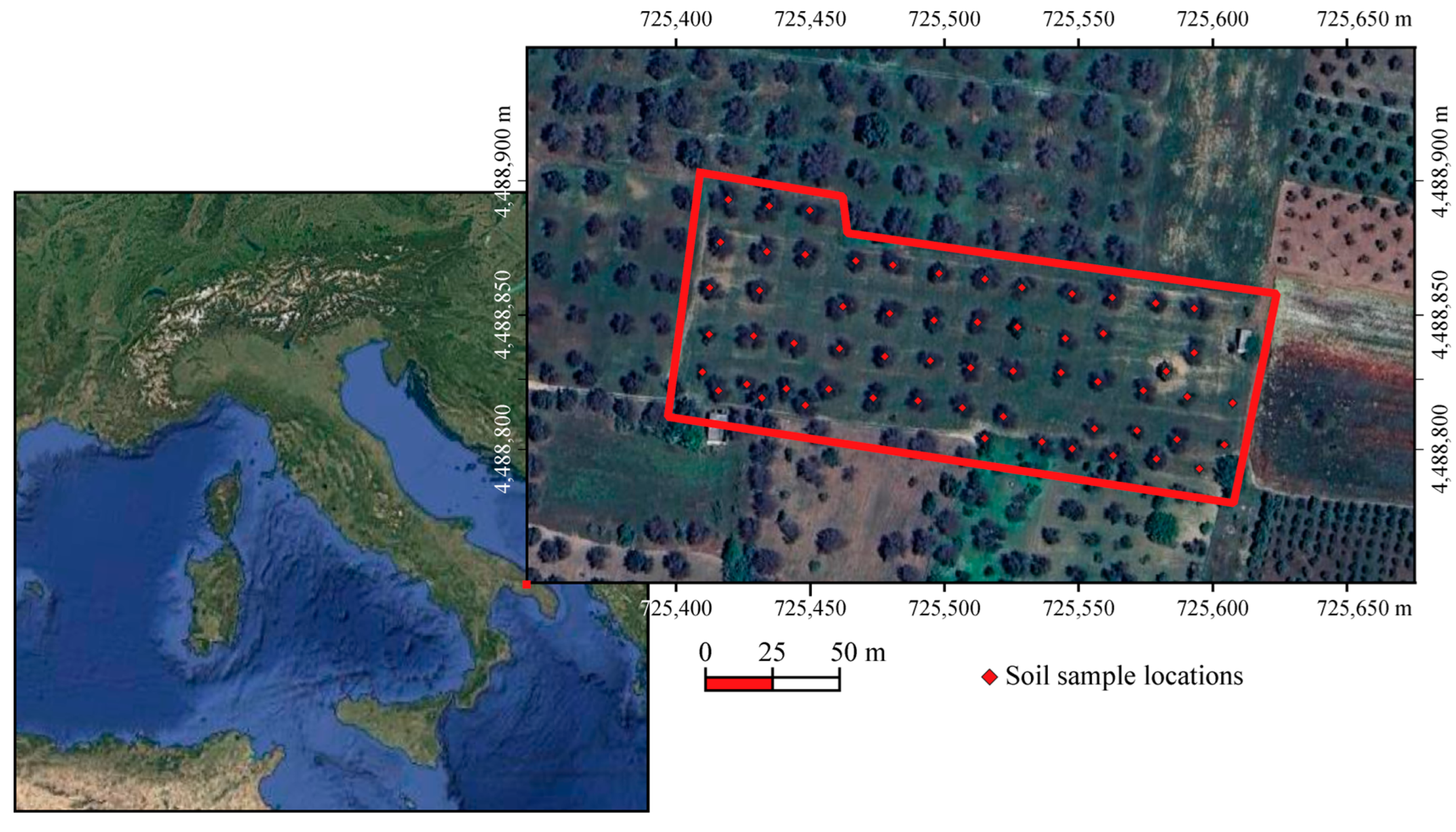
Figure 2.
Planet reflectance bands after the filtering of the soil data because of the screen operated by the olive tree canopies (a); The soil map at 1m resolution after applying deconvolution by kriging of Planet bands (b).
Figure 2.
Planet reflectance bands after the filtering of the soil data because of the screen operated by the olive tree canopies (a); The soil map at 1m resolution after applying deconvolution by kriging of Planet bands (b).
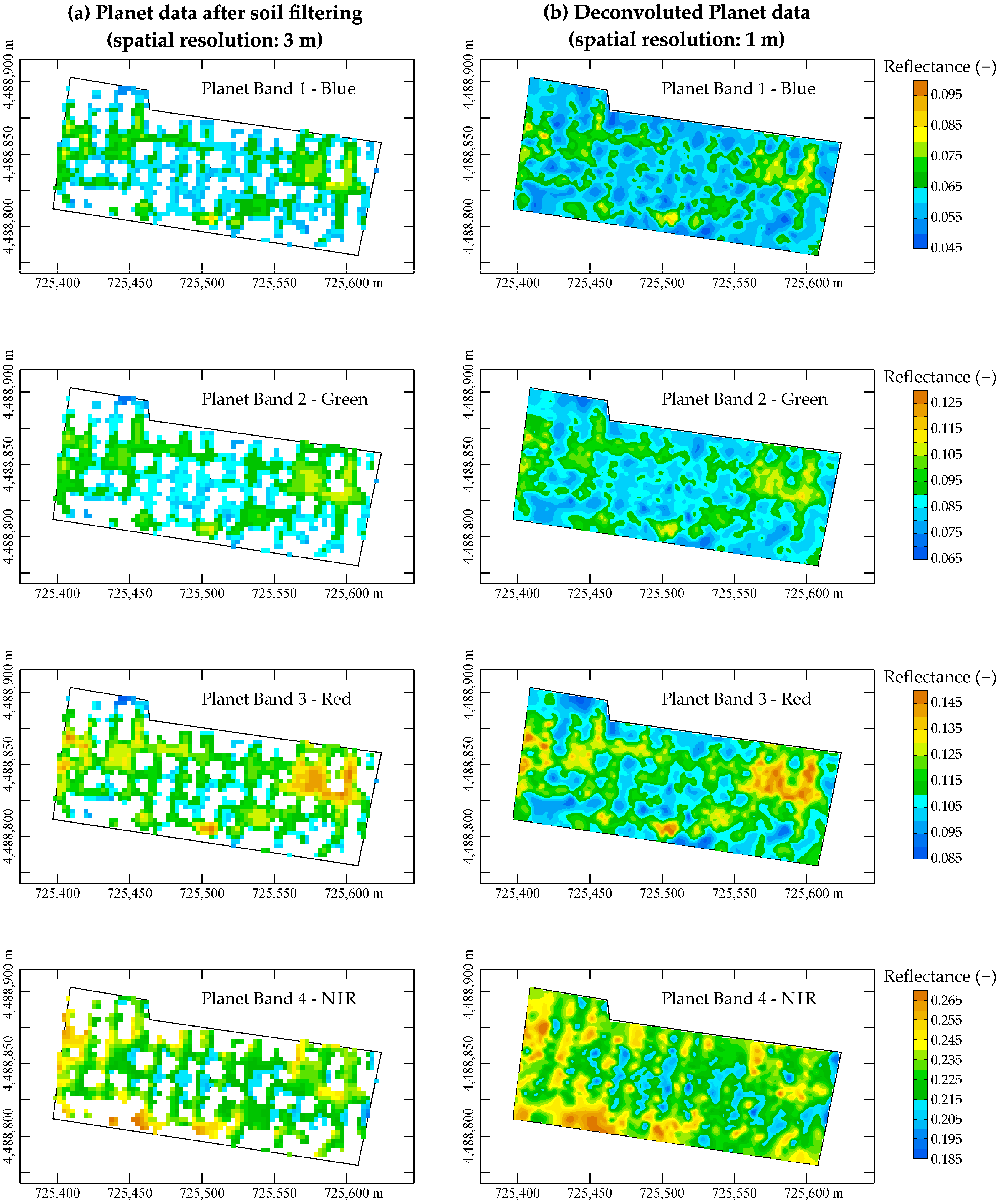
Figure 3.
The soil map at 1 m resolution after applying deconvolution by kriging of B11-B12 Sentinel2 bands.
Figure 3.
The soil map at 1 m resolution after applying deconvolution by kriging of B11-B12 Sentinel2 bands.
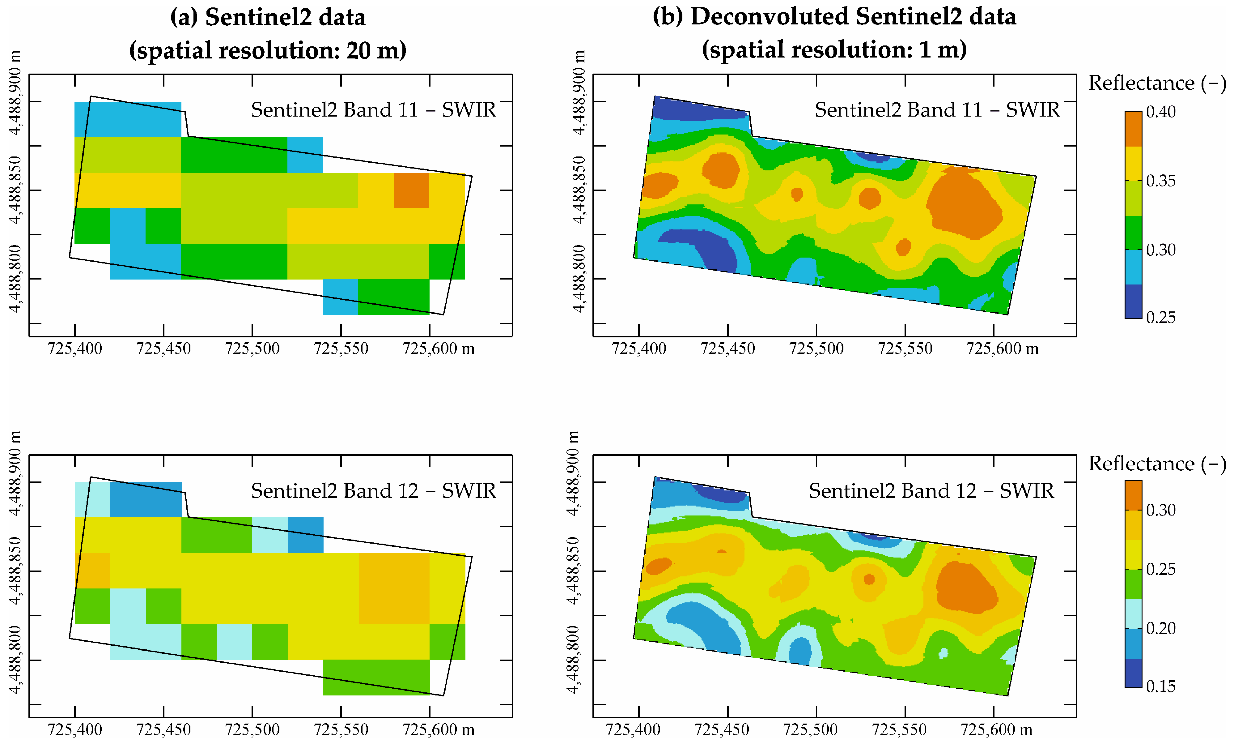
Figure 4.
Linear model of coregionalization (LMC) of the UAV multispectral data. The plotted black points are the experimental values whereas the solid red lines are the model of coregionalization. The green lines are the hull of perfect correlation while the horizontal dashed lines are the experimental variances.
Figure 4.
Linear model of coregionalization (LMC) of the UAV multispectral data. The plotted black points are the experimental values whereas the solid red lines are the model of coregionalization. The green lines are the hull of perfect correlation while the horizontal dashed lines are the experimental variances.
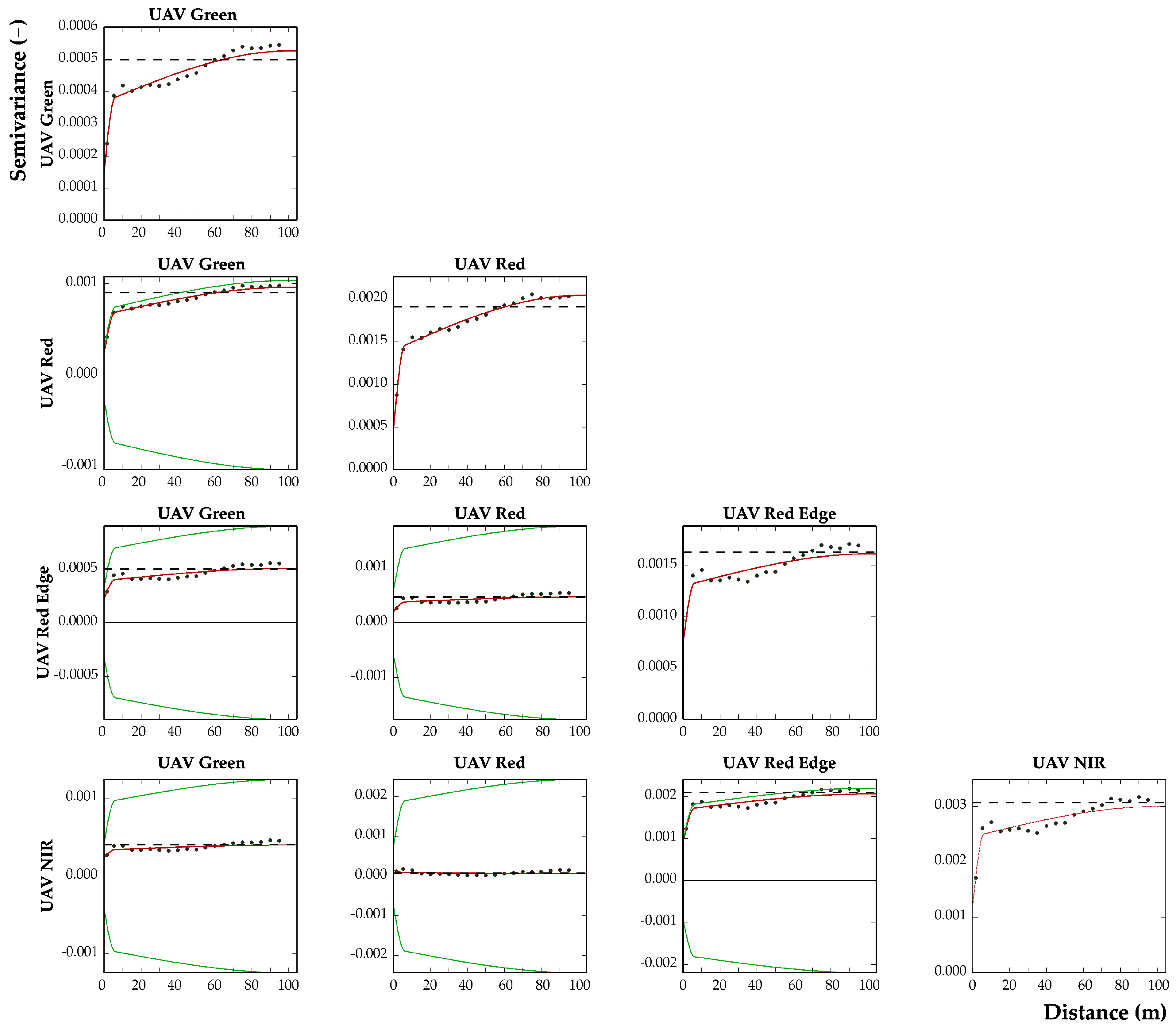
Figure 5.
The application of block cokriging produced the soil images of the UAV multispectral data.
Figure 5.
The application of block cokriging produced the soil images of the UAV multispectral data.
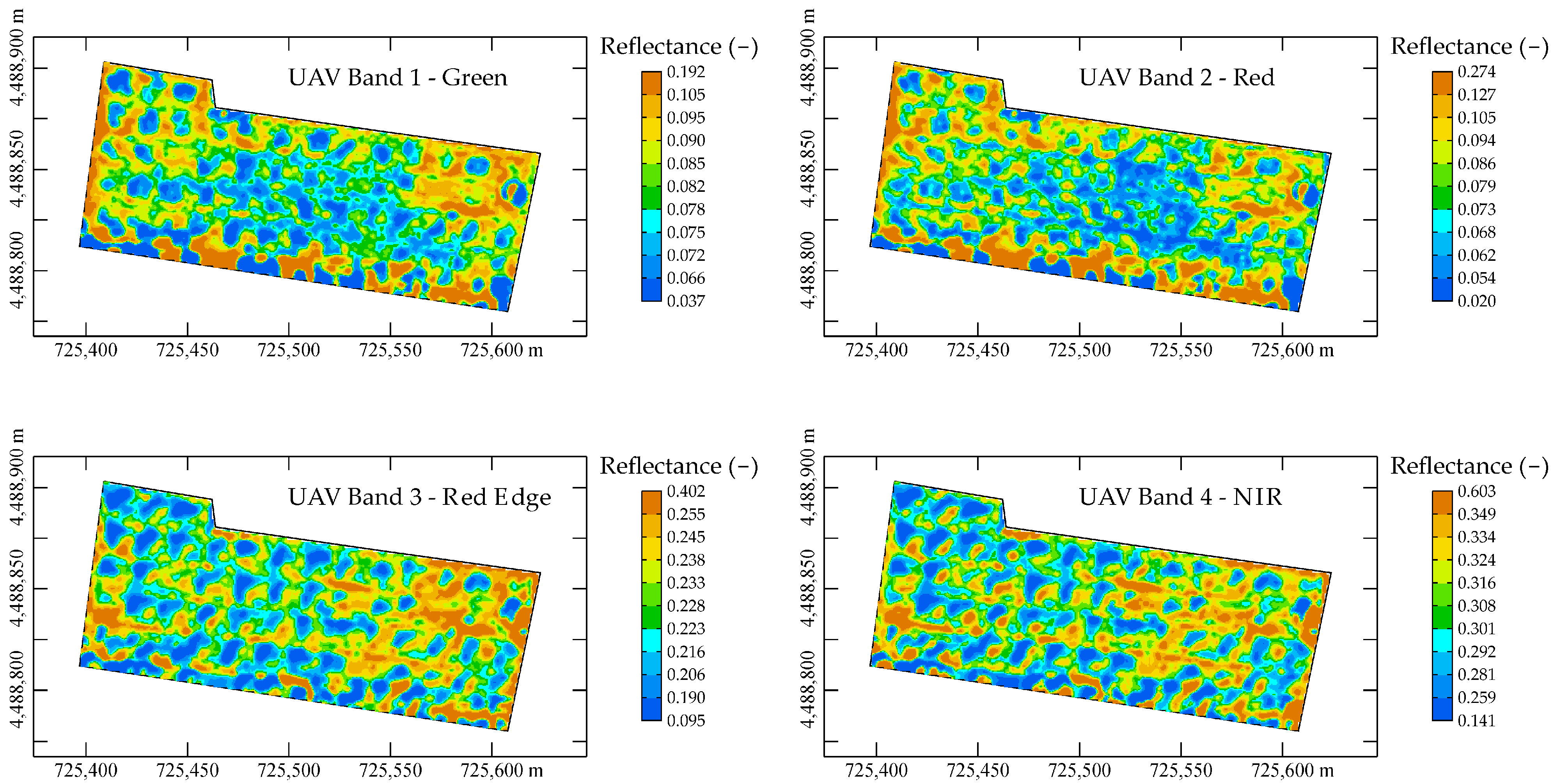
Figure 6.
Direct variograms of the fusion data set. The plotted black points are the experimental values whereas the solid red lines are the model of coregionalization. The horizontal dashed lines are the experimental variances.
Figure 6.
Direct variograms of the fusion data set. The plotted black points are the experimental values whereas the solid red lines are the model of coregionalization. The horizontal dashed lines are the experimental variances.
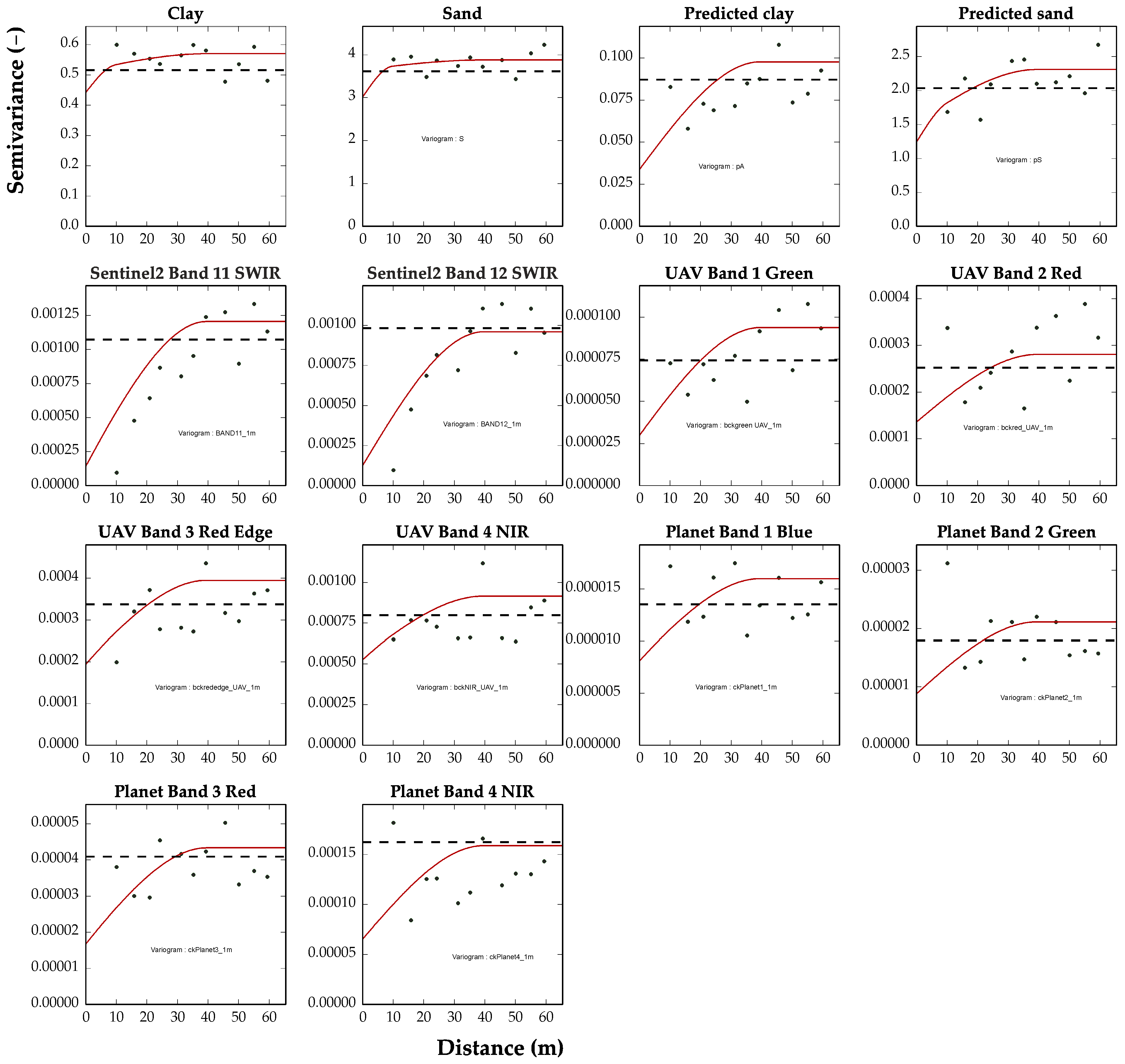
Figure 7.
Cross variograms of the fusion data set. The plotted black points are the experimental values whereas the solid red lines are the model of coregionalization. The green lines are the hull of perfect correlation while the horizontal dashed lines are the experimental variances.
Figure 7.
Cross variograms of the fusion data set. The plotted black points are the experimental values whereas the solid red lines are the model of coregionalization. The green lines are the hull of perfect correlation while the horizontal dashed lines are the experimental variances.
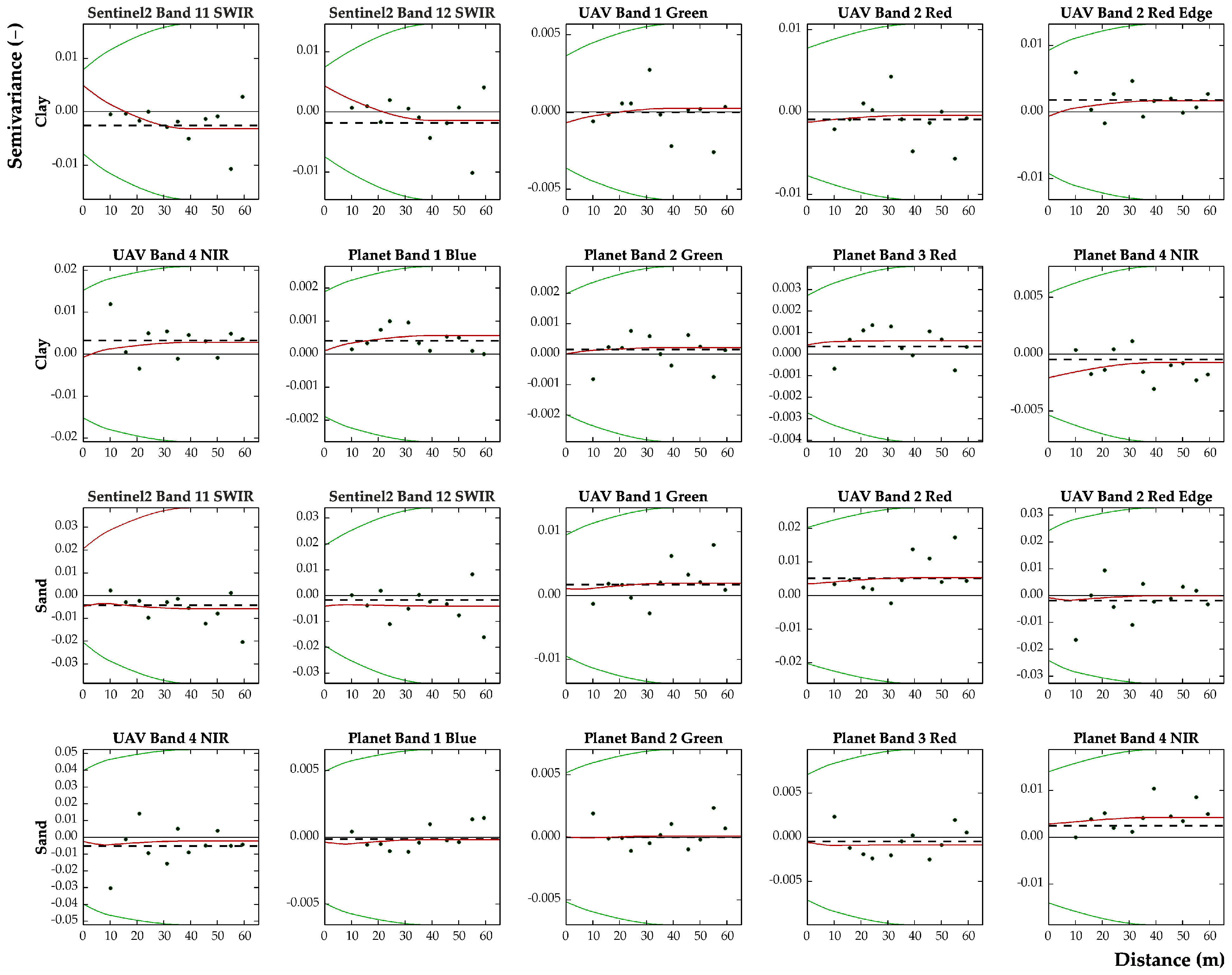
Figure 8.
Maps of clay and sand using the data fusion of all variables (a) and univariate ordinary kriging (b).
Figure 8.
Maps of clay and sand using the data fusion of all variables (a) and univariate ordinary kriging (b).
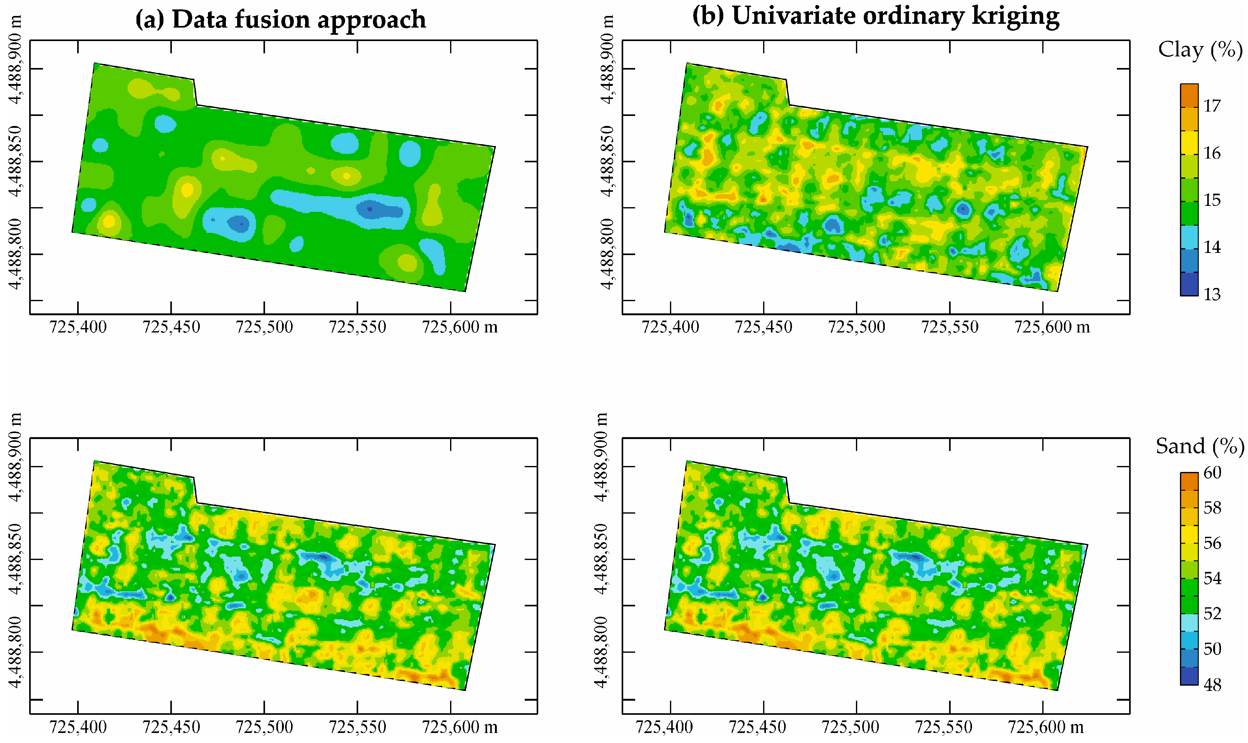
Figure 10.
Variograms of clay and sand. The plotted black points are the experimental values whereas the solid red lines are the fitted theoretical variogram models. The horizontal dashed lines are the experimental variances.
Figure 10.
Variograms of clay and sand. The plotted black points are the experimental values whereas the solid red lines are the fitted theoretical variogram models. The horizontal dashed lines are the experimental variances.
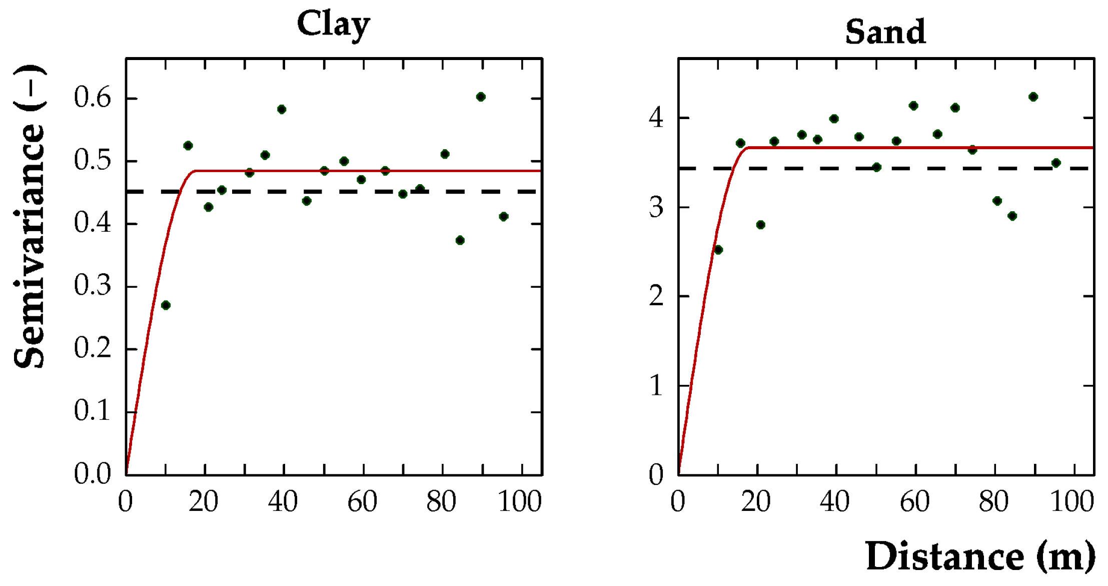
Figure 11.
Maps of kriging standard deviation for clay and sand using the data fusion of all variables (a) and univariate ordinary kriging (b).
Figure 11.
Maps of kriging standard deviation for clay and sand using the data fusion of all variables (a) and univariate ordinary kriging (b).
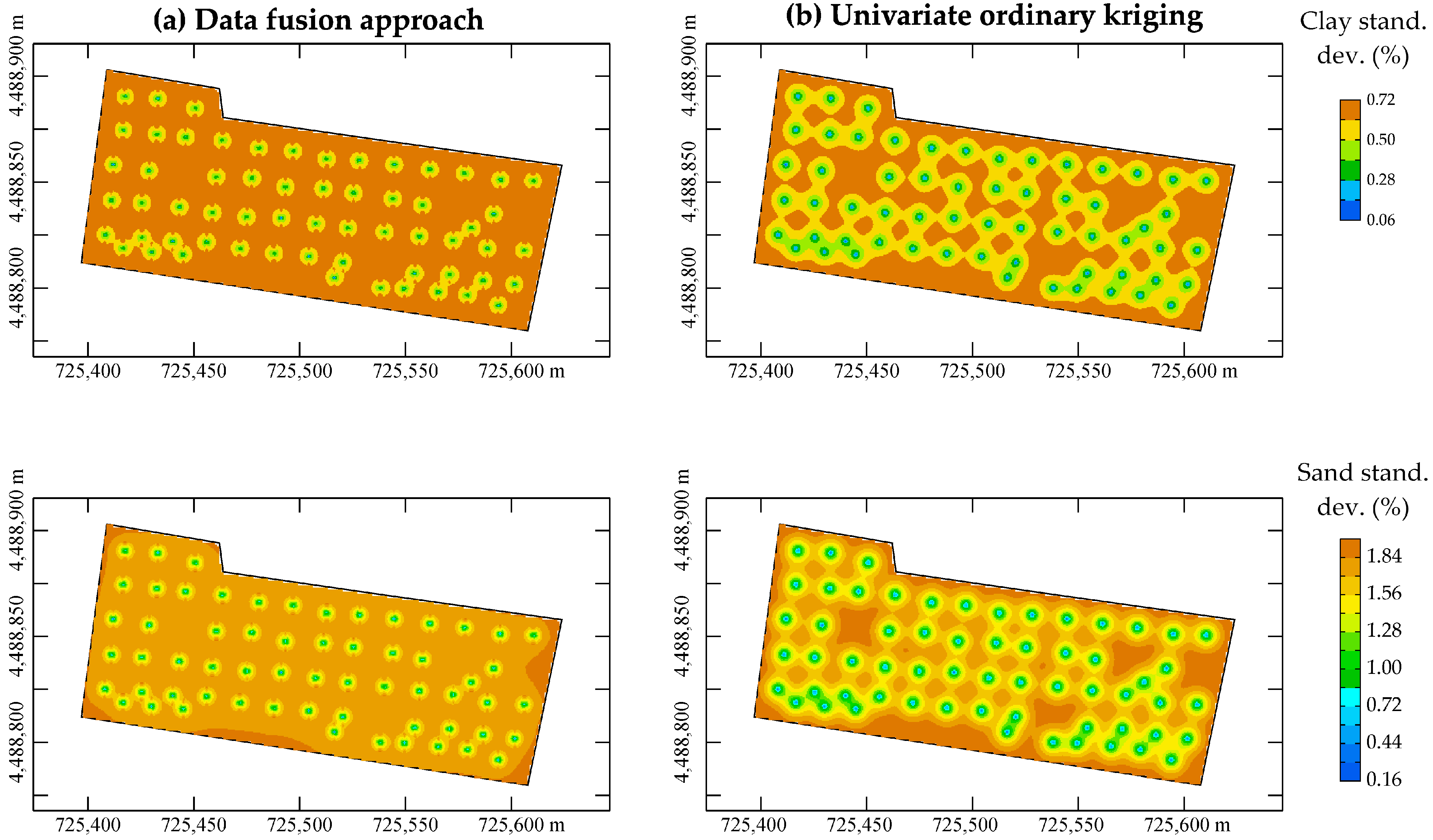

Table 1.
Remote sensing products used in this research.
| Satellite | Date | Band | Central wavelength (nm) |
Spatial Resolution (m) |
|---|---|---|---|---|
| UAV | 20190802 | Band 1 Green - VIS | 550 | 0.07 |
| Band 2 Red - VIS | 660 | |||
| Band 3 Red Edge - VIS | 735 | |||
| Band 4 - NIR | 790 | |||
| Planet | 20190721 | Band 1 Blue - VIS | 455 | 3.00 |
| Band 2 Green VIS | 500 | |||
| Band 3 Red - VIS | 590 | |||
| Band 4 - NIR | 780 | |||
| Sentinel 2 | 20190724 | Band 11 - SWIR | 1610 | 20.00 |
| Band 12 - SWIR | 2190 |
Table 2.
Statistical properties of the prediction models with R2> 0.5 with exception for silt and the results of residual analysis.
Table 2.
Statistical properties of the prediction models with R2> 0.5 with exception for silt and the results of residual analysis.
| Response variable (Y) | Type of Spectrum | Rangea (nm) |
Differentiationb | Pre-processingc | RMSEP (%) |
R2 (-) |
RIPQ (-) |
Wd | Pr<W | De | Pr>D |
|---|---|---|---|---|---|---|---|---|---|---|---|
| Clay | R | s | Raw | 0.41 | 0.68 | 2.28 | 0.98 | 0.31 | 0.08 | >0.15 | |
| Clay | R | s | no | SG | 0.36 | 0.75 | 2.59 | 0.98 | 0.36 | 0.09 | >0.15 |
| Sand | R | f | no | SG | 1.23 | 0.59 | 2.69 | 0.96 | 0.07 | 0.11 | 0.09 |
| Sand | R | s | Raw | 1.28 | 0.56 | 2.59 | 0.99 | 0.84 | 0.05 | >0.150 | |
| Silt | R | s | Raw | 1.13 | 0.35 | 1.86 | 0.96 | 0.06 | 0.11 | 0.09 |
af indicates full range and s selected ranges; bDifferentiation: 1a and 2a derivative; cPre-processing method: MSC = Multiplicative scatter correction; SNV = Standard normal variate; SG = denoising-smoothing method of Savitzky–Golay; dW of Shapiro-Wilk test; eD of Kolmogorov-Smirnov.
Table 3.
Structural analysis of RS data.
| Band | Support ratio | Variogram | ||
| Model | Parameter | |||
| Sill (-) | Range (m) | |||
| Planet Band 1 | 0.33 | Nugget effect | 366.49 | - |
| Spherical | 1181.69 | 8.48 | ||
| Spherical | 1544.04 | 33.97 | ||
| Planet Band 2 | 0.33 | Nugget effect | 62.09 | - |
| Spherical | 1730.09 | 17.70 | ||
| Spherical | 2498.13 | 40.15 | ||
| Planet Band 3 | 0.33 | Nugget effect | 526.90 | - |
| Spherical | 2601.90 | 20.00 | ||
| Spherical | 6280.06 | 40.00 | ||
| Planet Band 4 | 0.33 | Nugget effect | 0.00 | - |
| Spherical | 5864.35 | 13.00 | ||
| Spherical | 9449.09 | 52.00 | ||
| Sentinel2 B11 and B12* | 0.05 | Spherical | 0.0007a | 57.04 |
| 0.0006b | ||||
| 0.0006c | ||||
| * Sentinel2 data have been analyzed using a multivariate approach and have a linear model of coregionalization including a direct variogram for each band (B11 and B12) and a cross-variogram for the pair of bands (B11 x B12) with a spherical model with the same range. The sill values are provided by a 2x2 variance-covariance matrix with the following elements (sills): B11-B11a = 0.0007; B11-B12= B12-B11b= 0.0006; B12-B12 c = 0.0006. | ||||
Table 4.
The basic statistics of multivariate data set.
| Variable | Min. | Median | Mean | Max. | Stand. Dev. | Skewness (-) | Kurtosis (-) |
|---|---|---|---|---|---|---|---|
| Clay (%) | 13.34 | 14.91 | 14.94 | 16.48 | 0.72 | 0.00 | 2.50 |
| Sand (%) | 51.19 | 54.82 | 54.90 | 57.98 | 1.90 | -0.12 | 1.79 |
| Predicted clay (%) | 14.20 | 15.00 | 14.94 | 15.65 | 0.30 | -0.06 | 2.97 |
| Predicted sand (%) | 51.23 | 54.73 | 54.90 | 57.86 | 1.43 | -0.28 | 2.92 |
| UAV Band 1 Green (-) | 0.05 | 0.07 | 0.07 | 0.10 | 0.01 | 0.69 | 3.43 |
| UAV Band 2 Red (-) | 0.04 | 0.06 | 0.07 | 0.11 | 0.02 | 0.96 | 3.95 |
| UAV Band 3 Red Edge (-) | 0.16 | 0.20 | 0.21 | 0.25 | 0.02 | -0.14 | 3.22 |
| UAV Band 4 NIR (-) | 0.22 | 0.29 | 0.29 | 0.39 | 0.03 | 0.47 | 4.75 |
| Planet Band 1 Blue (-) | 0.05 | 0.06 | 0.06 | 0.07 | 0.00 | 0.36 | 2.89 |
| Planet Band 1 Green (-) | 0.08 | 0.08 | 0.08 | 0.10 | 0.00 | 1.20 | 4.57 |
| Planet Band 3 Red (-) | 0.09 | 0.11 | 0.11 | 0.12 | 0.01 | 0.87 | 4.00 |
| Planet Band 4 SWIR (-) | 0.21 | 0.23 | 0.23 | 0.27 | 0.01 | 0.31 | 2.94 |
| Sentinel2 Band 11 SWIR (-) | 0.26 | 0.33 | 0.33 | 0.39 | 0.03 | -0.30 | 2.36 |
| Sentinel2 Band 12 SWIR (-) | 0.18 | 0.25 | 0.25 | 0.31 | 0.03 | -0.36 | 2.62 |
Table 5.
Correlation matrix between primary variables and auxiliary variables.
| Clay | Sand | Predicted clay | Predicted sand | UAV Band 1 Green | UAV Band 2 Red | UAV Band 3 Red Edge | UAV Band 4 NIR | Planet Band 1 Blue | Planet Band 1 Green | Planet Band 3 Red | Planet Band 4 SWIR | Sentinel2 Band 11 SWIR | Sentinel2 Band 12 SWIR | |
|---|---|---|---|---|---|---|---|---|---|---|---|---|---|---|
| Clay | 1.00 | -0.82 | 0.41 | -0.58 | 0.00 | -0.08 | 0.14 | 0.16 | 0.15 | 0.05 | 0.08 | -0.05 | -0.11 | -0.08 |
| Sand | -0.82 | 1.00 | -0.33 | 0.75 | 0.11 | 0.17 | -0.05 | -0.10 | -0.02 | 0.00 | -0.04 | 0.10 | -0.07 | -0.03 |
| Predicted clay | 0.41 | -0.33 | 1.00 | -0.31 | 0.01 | -0.07 | 0.14 | 0.15 | 0.09 | 0.04 | 0.05 | 0.03 | -0.32 | -0.37 |
| Predicted sand | -0.58 | 0.75 | -0.31 | 1.00 | 0.13 | 0.21 | -0.03 | -0.06 | -0.01 | -0.06 | -0.10 | 0.04 | -0.01 | -0.01 |
| UAV Band 1 Green | 0.00 | 0.11 | 0.01 | 0.13 | 1.00 | 0.91 | 0.55 | 0.28 | -0.32 | 0.36 | 0.35 | 0.19 | 0.09 | 0.16 |
| UAV Band 2 Red | -0.08 | 0.17 | -0.07 | 0.21 | 0.91 | 1.00 | 0.23 | -0.03 | 0.28 | 0.27 | 0.27 | 0.18 | 0.04 | 0.11 |
| UAV Band 3 Red Edge | 0.14 | -0.05 | 0.14 | -0.03 | 0.55 | 0.23 | 1.00 | 0.93 | 0.28 | 0.31 | 0.26 | 0.25 | 0.04 | 0.07 |
| UAV Band 4 NIR | 0.16 | -0.10 | 0.15 | -0.06 | 0.28 | -0.03 | 0.93 | 1.00 | 0.25 | 0.22 | 0.12 | 0.33 | -0.12 | -0.10 |
| Planet Band 1 Blue | 0.15 | -0.02 | 0.09 | -0.01 | 0.32 | 0.28 | 0.28 | 0.25 | 1.00 | 0.81 | 0.80 | 0.49 | -0.05 | 0.01 |
| Planet Band 1 Green | 0.05 | 0.00 | 0.04 | -0.06 | 0.36 | 0.27 | 0.31 | 0.22 | 0.81 | 1.00 | 0.91 | 0.43 | 0.25 | 0.29 |
| Planet Band 3 Red | 0.08 | -0.04 | 0.05 | -0.10 | 0.35 | 0.27 | 0.26 | 0.12 | 0.80 | 0.91 | 1.00 | 0.21 | 0.40 | 0.44 |
| Planet Band 4 SWIR | -0.05 | 0.10 | 0.03 | 0.04 | 0.19 | 0.18 | 0.25 | 0.33 | 0.49 | 0.43 | 0.21 | 1.00 | -0.27 | -0.22 |
| Sentinel2 Band 11 SWIR | -0.11 | -0.07 | -0.32 | -0.01 | 0.09 | 0.04 | 0.04 | -0.12 | -0.05 | 0.25 | 0.40 | -0.27 | 1.00 | 0.96 |
| Sentinel2 Band 12 SWIR | -0.08 | -0.03 | -0.37 | -0.01 | 0.16 | 0.11 | 0.11 | -0.10 | 0.01 | 0.29 | 0.44 | -0.22 | 0.96 | 1.00 |
Table 6.
Cross validation results for clay and according to the two approaches. ME=mean error; RMSSE= Root Mean Squared Standardized Error; RMSE=root mean squared error; R coefficient of determination between measured and estimated values; ρ= correlation coefficient between the standardized error and the estimate.
Table 6.
Cross validation results for clay and according to the two approaches. ME=mean error; RMSSE= Root Mean Squared Standardized Error; RMSE=root mean squared error; R coefficient of determination between measured and estimated values; ρ= correlation coefficient between the standardized error and the estimate.
| Variable | Approach | ME (%) |
RMSSE (%) |
RMSE (%) |
R2(-) |
r (-) |
|---|---|---|---|---|---|---|
| Clay | Univariate | -0.0130 | 1.09 | 0.1803 | n.s.* | 0.42 |
| Data fusion | 0.0016 | 1.14 | 0.0021 | 0.85 | 0.12 | |
| Sand | Univariate | 0.0298 | 1.02 | 0.0118 | n.s. | 0.21 |
| Data fusion | 0.0016 | 1.09 | 0.0037 | 0.89 | 0.09 |
* n.s. means not statistically different from zero.
Disclaimer/Publisher’s Note: The statements, opinions and data contained in all publications are solely those of the individual author(s) and contributor(s) and not of MDPI and/or the editor(s). MDPI and/or the editor(s) disclaim responsibility for any injury to people or property resulting from any ideas, methods, instructions or products referred to in the content. |
© 2024 by the authors. Licensee MDPI, Basel, Switzerland. This article is an open access article distributed under the terms and conditions of the Creative Commons Attribution (CC BY) license (http://creativecommons.org/licenses/by/4.0/).
Copyright: This open access article is published under a Creative Commons CC BY 4.0 license, which permit the free download, distribution, and reuse, provided that the author and preprint are cited in any reuse.


