
Submitted:
11 November 2024
Posted:
29 November 2024
You are already at the latest version
Abstract
Existing vehicle travel time prediction applications face two primary challenges: modeling complex road network structures and handling irregular spatio=emporal traffic state propagation. To address these challenges, this paper proposes a novel travel time prediction method, GMTP, based on vehicle GPS data. The proposed GMTP method improves the original attention mechanism ,by introducing shared attention mechanism with high computational efficiency, and integrates the graph attention network GATv2 and the long sequence language model BERT. This enables the adaptive analysis of dynamic correlations between road segments across broad spatial and temporal dimensions. The pre-training process of the model consists of two blocks. In the first block, a segment interaction pattern-enhanced graph attention network is employed to convert road network structural features and interaction semantics into road segment representation vectors. In the second block, a traffic congestion-aware trajectory encoder maps these road segment representations to trajectory representation vectors incorporating traffic time characteristics for encoding. Additionally, two self-supervised tasks are designed: adaptive masked trajectory reconstruction task and trajectory contrastive learning, which aims to enhance the model’s accuracy and robustness. Finally, the model is fine-tuned on two large-scale real-world trajectory datasets to validate its effectiveness. Experimental results demonstrate that the proposed method generalizes well across different cities and adapts to heterogeneous trajectory datasets. Moreover, key evaluation metrics such as MAE, MAPE, and RMSE are significantly reduced, and computational efficiency is improved.
Keywords:
Road Network
; GATv2
; BERT
; Travel Time Prediction
1. Introduction
With the continuous advancement of satellite positioning technology, both the global positioning system (GPS) and Beidou high-precision positioning system are being increasingly applied in outdoor environments. These technologies not only enable real-time acquisition of users’ precise location information, but also provide a robust data foundation for various applications. The widespread adoption of positioning technology has generated amounts of spatiotemporal trajectory data, which typically includes valuable information such as traffic flow, user behavior, and environmental factors. As a result, effectively utilizing this data for tasks, such as trajectory-based prediction[1,2]traffic flow prediction [3,4], urban hazardous materials management [5], trajectory similarity calculation [6] ,has become a hot topic in the data engineering field.
Travel time prediction (TTP) is a critical component of many trajectory prediction tasks and an essential feature in numerous mobile map applications. For example, Baidu Maps, one of the world’s largest mobile map platforms, serves over 340 million monthly active users [7].Accurate TTP plays a vital role in road navigation, route optimization, cargo transportation monitoring, and fatigue driving prevention. In the context of cargo transportation, real-time TTP enables users to anticipate traffic conditions, optimize route planning, avoid congestion, and ensure timely delivery of goods. Additionally, when unexpected events occur during the journey, TTP can help users swiftly adjust routes, saving both transportation time and costs [8]. Thus, providing a precise and reliable TTP module is crucial for improving transportation efficiency and reducing operational expenses.
TTP is influenced by various factors, including traffic congestion, departure time, weather conditions, and individual driver preferences. Previous research often struggles to make accurate predictions due to the complexity of these factors. However, with the advent of deep learning, large-scale trajectory datasets have been increasingly utilized for model training, allowing for the extraction and use of spatiotemporal correlation patterns in trajectory sequences. Additionally, in areas with complex road network, effective travel time prediction requires not only high-performance models but also a thorough consideration of spatiotemporal correlations at the road network level. Therefore, developing accurate, efficient, and reliable travel time prediction models is of significant practical value, contributing to improved performance and user experience in map applications. In travel time prediction, mining spatiotemporal correlation features help models better capture the temporal irregularities and spatial dependencies in trajectory data, such as the contextual information between road segments and the temporal characteristics of traffic flow. Traditional road segment-based prediction methods[9,10,11] typically predict the travel time for each road segment independently and then sum these predictions to calculate the total travel time. Although this approach is computationally efficient, its accuracy decreases as the path length increases, and it often overlooks important contextual information like traffic lights and turns, limiting its overall precision.
To address these shortcomings, end-to-end methods have been developed [12,13] , which treat all road segments in a trajectory as a unified whole, capturing the contextual relationships between road segments using recurrent structures. However, the computational cost of these cyclic structures increases significantly as the number of road segments grows, restricting their real-time processing capabilities.
In response to these limitations, researchers have introduced deep learning models that combine various neural network architectures to handle complex data for travel time prediction. For example, the convolutional spatiotemporal graph attention network (STGAT) proposed in [14] transforms road networks into low-dimensional vectors and captures spatial information by setting an appropriate convolutional network size, thereby enhancing travel time prediction accuracy. Additionally, Wang [15] proposed a neural network-based model that integrates spatiotemporal features,traffic characteristics, and personalized factors. This model, comprising a shallow linear layer, a deep neural network, and a recurrent neural network, outperforms the WD (wide and deep) [16]model by more effectively mining local road segment information.
However, while these methods address the correlation between road segments to some extent, they still fail to fully explore the complex temporal patterns embedded in trajectories. Studies have shown that significant changes in trajectory data during morning and evening peak hours directly affect road congestion and trajectory formation. Irregular time intervals also reveal another temporal dimension of trajectories. In response, [17] proposed a novel self-supervised trajectory representation learning framework, which incorporates time patterns and travel semantics into trajectory learning through a two-stage process, significantly improving downstream prediction tasks. Nevertheless, this model is complex, and the number of parameters increases substantially as the model grows in complexity. Therefore, while improving model performance, reducing the number of parameters required for training remains an important direction for further optimization.
Many existing methods use spatiotemporal graph neural networks to improve the accuracy of travel time prediction, but certain limitations remain. First, most methods treat temporal and spatial features separately, failing to fully explore the correlations between the two. Second, these models tend to overlook changes in traffic congestion, leading to a significant decrease in prediction accuracy in complex traffic environments. To address these challenges, this paper proposes a spatiotemporal feature deep learning framework for travel time prediction based on an improved attention mechanism, called GMTP. This framework integrates GATv2 and BERT to capture contextual relationships and spatiotemporal correlations within road network data. It also leverages an adaptive spatiotemporal attention mechanism to extract temporal features from trajectories, enabling the accurate detection of traffic congestion changes. Additionally, the framework introduces MLM-based trajectory reconstruction tasks and contrastive learning tasks to further enhance the pre-training model, allowing it to fully capture the spatiotemporal characteristics of trajectory data. Finally, by fine-tuning downstream tasks, the framework achieves more accurate travel time prediction results.
• Introduced a high-performance spatiotemporal graph attention network (GATv2): Constructed a road segment interaction frequency matrix to fully leverage the spatial and temporal correlations for modeling complex road network structures. This approach deeply integrates with BERT, effectively capturing complex interaction relationships between nodes, and enhancing the model’s ability to analyze spatiotemporal dynamic features.
• Proposed a head information sharing spatiotemporal self-attention mechanism (HSSTA):This mechanism learns contextual information in trajectories by extracting traffic time characteristics such as peak hours and weekdays in the attention layer. A hybrid matrix is introduced in the attention head to adaptively adjust attention layer parameters, improving both computational efficiency and prediction accuracy.
• Designed an adaptive self-supervised learning task:This task reconstructs trajectory sequences by gradually increasing the masking ratio of trajectory subsequences. Combined with contrastive learning, this method reduces interference from other related information, increases the difficulty of true value prediction, and enhances the cross-sequence transferability of the pre-trained model, improving its generalization and robustness.
• Conducted experiments on two real-world trajectory datasets: The results demonstrate that the proposed method significantly outperforms other methods in both performance and computational efficiency.
2. Related Work
2.1. Spatiotemporal Graph Neural Networks
Graph neural networks (GNNs) [26] have been extensively applied in graph-based tasks such as traffic network analysis, knowledge graph creation, recommendation systems, and other domains that leverage graph structures. Their ability to handle non-Euclidean spatial data and complex features makes them highly effective in these areas. Advanced GNNs can generally be classified into four main types: recurrent graph neural networks (RecGNNs), convolutional graph neural networks (ConvGNNs), graph autoencoders (GAEs), and spatiotemporal graph neural networks (STGNNs).
To account for temporal dependencies, DLSTM [27] and GWN [28] introduced prediction frameworks built on recurrent neural networks (RNNs) and temporal convolutional networks (TCNs), respectively. GMAN [29] and STGNN [30] leverage temporal self-attention mechanisms to enhance long-term temporal learning. In comparison to traditional GNNs, STAN [31] incorporates an inter-region correlation model utilizing the graph attention network (GAT) [20] . However, while these studies have exploited spatiotemporal features, they have not jointly modeled both dimensions.
To address this issue, this paper proposes an enhanced dynamic graph attention network, GATv2, designed to dynamically infer spatial and temporal features within graph structures while embedding the temporal characteristics of segment interaction frequencies into the segment representations. Compared to the GAT, GATv2 overcomes its limitations and more effectively captures complex spatiotemporal correlation patterns.
2.2. Transformer-Based Language Models
Transformer-based language models have achieved substantial advancements across various fields. These models are generally classified into three categories: encoder-decoder models ( T5 [32], BART [33]), encoder-only models (BERT [24], RoBERTa [34]), and decoder-only models (GPT-2 [35]). In recent years, decoder-based large language models (LLMs), particularly following the introduction of publicly available models like ChatGPT, have garnered significant attention. ChatGPT, through user feedback alignment, can effectively adapt to diverse tasks, accurately identify user intentions, and generate desired outcomes.
Following ChatGPT, several LLMs were released, including Llama2 [36] and Falcon [37]. While LLMs exhibit strong dialogue and interaction capabilities, their context-dependent learning strategies often underperform in specific tasks compared to fine-tuned, smaller-scale language models. Additionally, fine-tuning LLMs remains computationally intensive despite the introduction of more efficient parameter-tuning methods.
In light of these challenges, our study opts for the encoder-only BERT model, aiming to reduce computational costs by improving the attention layer to decrease the number of parameters. Simultaneously, fine-tuning the pre-trained model enhances training accuracy.
2.3. Self-Supervised Learning
The masked language model (MLM) is a fundamental component of the Transformer architecture and is widely employed in tasks such as text generation, machine translation, and sentiment analysis[43,44]. Its mechanism involves randomly masking certain words in a sentence, allowing the model to predict the masked words based on the remaining unmasked content.
Contrastive learning [38], a self-supervised learning framework, has been extensively applied in tasks related to visual representation [39] and natural language processing[40]. Contrastive Predictive Coding (CPC) [41]is a pioneering approach in deep contrastive learning, optimizing the feature extraction network by maximizing the similarity (i.e., consistency) between predicted and actual results in sequence data. It also introduced the InfoNCE loss function, which is now widely used in contrastive learning research. Khosla et al. [42] proposed the supervised contrastive learning loss (SCL Loss), extending contrastive learning into supervised learning, to enhance the model’s feature representation by utilizing labeled data.
Drawing inspiration from these studies, this research employs a data-augmented contrastive learning approach, leveraging anchor samples and the normalized cross-entropy loss function to identify trajectory samples that have undergone data augmentation.
3. Methodology
Figure 1 shows the architecture of the proposed framework GMTP,which consists of four modules: a segment interaction pattern-enhanced graph attention network,a traffic congestion-aware trajectory encoder, an adaptive masked trajectory reconstruction task, and a trajectory contrastive learning task.
3.1. Road Segment Interaction Model to Enhance GATv2
The segment interaction pattern-enhanced graph attention network employs a novel spatiotemporal graph attention mechanism to capture spatiotemporal correlations in complex traffic conditions, including factors such as segment interaction frequency and segment transition duration.
The Graph Attention Network (GAT)[20] is a widely used and advanced graph neural network (GNN) architecture in graph representation learning. GAT models the constraints between road segments in a road network by mapping them into a graph structure, allowing it to capture the spatial features of the network, which are then used as input to the model. By introducing a multi-head attention mechanism, GAT assigns distinct attention weights to each node and its neighboring nodes, enhancing the expressiveness of the attention layer. The model then generates a new representation vector for each road segment through a weighted summation of the nodes, effectively capturing the relationships and characteristics between road segments. Additionally, GAT employs a scoring function to compute a score for each edge , reflecting the importance of the features of the neighbor node j to node i:
where , are learned, and ∥ denotes vector concatenation. After calculating the attention scores for the node and all neighboring nodes, softmax is used for normalization:
Then, GAT computes a weighted average of the transformed features of the neighbor nodes (followed by a nonlinearity ) as the new representation of i, using the normalized attention coefficients:
In GAT, each node only attends to its neighboring nodes, using its representation as the query vector and the neighbors’ representations as the keys. This means that the order of attention scores does not change with variations in the node’s features. Consequently, the attention weights are static and do not dynamically adjust based on changes in node features. This approach is known as "static attention." However, in road networks, transition probabilities between segments are often uncertain, and interactions between nodes are complex. These factors may cause static attention to limit GAT’s ability to effectively fit training data in complex models.
To address these limitations, Brody[21] introduced GATv2, a variant of the graph neural network that implements dynamic attention by modifying the order of operations. In the standard GAT scoring function,the learned layers and are performed sequentially, which can lead the attention layer to collapse into a linear layer. GATv2 applies the layer after the nonlinearity (LeakyReLU), and the layer after the concatenation, effectively applying an MLP to compute the score for each query-key pair. This modification theoretically enhances the GATv2 to better fit training data.
- GATv2:
Additionally, GATv2 introduces a segment interaction frequency matrix computed from historical data, to account for factors like user preferences and traffic conditions. This matrix expands the calculation of attention weights by integrating temporal and spatial characteristics of the road network. As a result, the model can more comprehensively and accurately capture spatiotemporal correlations within the road network, allowing it to adapt more effectively to complex road environments.
- GATv2-Enhanced:
where are road representations of and , are learnable parameters, LeakyReLU is the activation function whose negative input slope is 0.2 [20], and is the interaction frequency between and , which can be calculated as:
where and are the frequency of edges and road appearing in the trajectory dataset , respectively.
GATv2 takes into account the complex interactions caused by static road network structure and human mobility and finally represents the road segments containing spatiotemporal feature information as vector outputs. Since the attention weights generated by GATv2 are dynamic, each node has a different attention weight ranking, making it more expressive than GAT. In addition, this dynamic attention mechanism is more robust to noise.
3.2. Traffic Congestion Aware Trajectory Encoder
With the ongoing advancements in natural language processing (NLP), technologies like LSTM [22], Transformer [23], and BERT [24] have been introduced and widely applied in various research areas. BERT, as a bidirectional encoder built on the Transformer architecture, effectively captures contextual information from both sides of a trajectory, facilitating comprehensive interaction between roads. Therefore, our work adopts BERT as the foundational model for training in the trajectory encoding layer.
After obtaining the segment representation sequences from the GATv2 layer, the next step is to convert these sequences into trajectory representations in the trajectory encoding layer while introducing a head information-sharing attention mechanism. Additionally, a traffic congestion sensor is designed to capture changes in road congestion by incorporating time semantics such as peak hours and weekdays. The trajectory encoding layer consists of two components: the trajectory cycle time refinement module and the adaptive shared attention module. Together, these components enable the model to more comprehensively and accurately understand and analyze the spatiotemporal characteristics of the road network.
3.2.1. Trajectory Cycle Time Refinement Module
This module utilizes week and day as time dimensions to capture the periodic traffic flow patterns on workdays. For each timestamp associated with road segment , vectors and are used to refine into corresponding periodic indices. Specifically, represents the workday index, while denotes the minute index. Finally, by integrating the embedded representation of the road segment with the traffic period, a fused road segment vector representation is obtained:
where represents the road segment vector, and are the corresponding time representations, and is the positional encoding of the trajectory data. Finally, the concatenated road segment vector representations are combined to form the initial vector representation X of trajectory T:
3.2.2. Adaptive Shared Attention Module
This module extracts segment transition durations within the same trajectory based on historical data, reflecting traffic congestion during peak hours. A hybrid matrix is introduced in this module, enabling simultaneous learning of key and query projections for all heads and allowing each head to adaptively reweight these projections, thus enhancing the expressive capacity of each head.
In the standard Transformer Encoder, self-attention is typically employed to learn the semantic information within the trajectory. Given an input trajectory representation, linear transformations are applied to generate the query matrix Q, key matrix K, and value matrix V, followed by the calculation of attention scores:
Firstly, to reflect the degree of road congestion, this module leverages historical data from peak periods to extract a transition duration matrix for each road segment, thereby capturing the interaction relationships between segments. On this basis, an adaptive matrix is introduced to represent the impact of different segments on the self-attention mechanism.
In the matrix , each element represents the weighting of the transition duration between segments and in the self-attention mechanism. If the transition time between segments is short, the value of is large, indicating that this segment pair has a stronger influence on self-attention. Conversely, if the transition time is longer, the influence of weakens accordingly.
For a given road segment with timestamp , the transition duration between any two segments is defined as . To process the transition duration, a logarithmic function is applied, where (where ). This ensures that as the transition duration increases, gradually decreases. Subsequently, a two-layer linear transformation is used to learn the transition time information between segments, effectively capturing the dynamic impact of transition duration on the relationship between segments:
where and are learnable parameters, and LeakyReLU is an activation function with a negative slope of 0.2 for negative inputs.
The attention score incorporating transition duration can be calculated as:
The Multi-Head Attention mechanism (MHA) generates the final output by concatenating the attention calculation results from each head. However, when training large-scale Transformer models, the attention layer may encounter the problem of over-parameterization. Jean-Baptiste Cordonnier[25] demonstrated that re-parameterizing pre-trained multi-head attention layers can effectively reduce the number of parameters in the attention layer, thus alleviating this issue.
Next, we introduce a hybrid matrix into the attention layer, which already incorporates spatiotemporal semantics. This hybrid matrix enables the simultaneous learning of key and query projections for all heads, allowing each head to adaptively reweight these projections, thereby enhancing the expressiveness of each head.
In this attention mechanism, each head does not independently generate key and query matrices but instead utilizes a shared mechanism. Each head learns a hybrid vector , which is projected onto dimension through shared matrices and , and a custom inner product operation is defined on the projection dimension.
Figure 2 illustrates the process of using a hybrid matrix in the attention mechanism for the input vectors, where the hybrid vectors are arranged in rows. The total dimension is defined, allocating a dimension for each head to ensure alignment with the dimension assigned to the i-th head. By learning the hybrid vectors , the expressiveness of each head is further enhanced. Typically, is set to 64, but it can be adjusted according to specific requirements, allowing each head to focus on larger or smaller feature spaces.
With this head information-sharing attention mechanism, the Transformer Encoder achieves the following benefits when constructing and training large-scale models:
- Enhanced Expressive Power: Each head can adaptively utilize the shared matrix to capture feature information across different dimensions, enabling richer representation within the attention mechanism.
- Reduced Parameter Redundancy: By sharing the projection matrix across heads, the total number of model parameters is significantly reduced, which improves computational efficiency.
- Flexible Head Configuration: This mechanism allows for head dimensions to be adjusted as needed, enabling the attention mechanism to flexibly adapt to varying levels of complexity.
3.2.3. Feedforward Network Layer
After the shared attention layer, a feedforward network layer with two linear transformations, activated by ReLU, is used to obtain the output representation Y of the trajectory T:
where and are two learnable parameters, while and are the biases for each respective layer.
3.3. Self-Supervised Pre-Training Tasks
During the model pre-training stage, an adaptive masked trajectory reconstruction task and a contrastive learning task are employed to strengthen the model’s ability to capture co-occurrence relationships between roads, the spatiotemporal characteristics of trajectories, and their semantic information.
3.3.1. Adaptive Masked Trajectory Reconstruction Task
Masked trajectory reconstruction creates a self-supervised pre-training task by concealing part of the input sample data and leveraging a neural network to reconstruct the masked portions. The BERT model has demonstrated that, through masked reconstruction tasks, a model can learn universal feature representations, thus enhancing performance on downstream tasks [19].
Given a trajectory T, in the initial training phase, we adopt a random masking strategy, masking parts of each trajectory sequence to help the model learn reconstruction capabilities from relatively simple contextual information. At this stage, the masking ratio is kept low, making it easier for the model to predict using the unmasked trajectory information. As training progresses, the masking ratio is gradually increased. Special markers and replace the corresponding position and timestamp to get the masked trajectory subsequence M.
After obtaining the representation of the masked trajectory T, a linear layer with parameters and is used to predict the masked sequence:
Next, the cross-entropy loss between the actual and predicted values of the masked sequence is used as the optimization objective:
Eventually, the masking ratio is gradually increased to cover a continuous subsequence of approximately of the total trajectory length. At this stage, the model can maintain robust trajectory reconstruction performance under a higher masking ratio, while significantly enhancing its ability to predict and transfer cross-sequence information.
3.3.2. Trajectory Contrastive Learning
Enhanced contrastive learning is a widely used framework that leverages data augmentation to generate different views of input samples, facilitating effective representation learning. The core principle is to maximize the similarity between views of the same sample while minimizing the similarity between views of different samples. In feature learning frameworks based on multi-view invariance, data augmentation is employed to capture multiple perspectives of the input samples. For data augmentation of trajectory sequences, both temporal dependency and variable dependency must be considered. Consequently, we adopt two data augmentation techniques—time-frequency perturbation and road segment masking—to create diverse views for contrastive learning.
Time-Frequency Perturbation: A subset of the trajectory sequence is randomly selected (with a ratio of ), and a noise factor is randomly added to this subset to generate a new sequence. The noise factor is defined as , where , and and represent the average travel times for the current and historical periods, respectively. By applying transformations to travel time, this method helps the model capture semantic information in the temporal dimension.
Road Segment Masking In the adaptive masked trajectory reconstruction task, portions of the trajectory sequence and temporal information are randomly masked. The masked segments can be regarded as missing values within the trajectory sequence, allowing the model to further learn the spatiotemporal correlations of the trajectory by predicting the missing parts.
Subsequently, we adopt the normalized temperature-scaled cross-entropy loss as the contrastive objective[45]. A random selection of trajectories is drawn from the dataset D, and after data augmentation, this yields trajectories. For each trajectory (referred to as an anchor point), we find the corresponding augmented trajectory (positive pair) from among the negative samples in each batch. The contrastive loss function for positive pairs is defined as follows:
Finally, the average value of is calculated to obtain the contrastive loss for learning, where is the temperature parameter, and represents the cosine similarity between and . The similarity function is defined as:
where is a training sample in the batch, and equals 1 if ; otherwise, it equals 0.
4. Results
This section may be divided by subheadings. It should provide a concise and precise description of the experimental results, their interpretation as well as the experimental conclusions that can be drawn.
4.1. Dataset Introduction
Our experiment uses two large-scale datasets: Porto and Beijing. The Porto dataset, from the Kaggle competition platform, contains open-source trajectory data collected from July 1, 2013, to July 1, 2014, with 435 user IDs and 695,085 trajectories (sampling frequency: 15 seconds). The Beijing dataset includes taxi trajectories recorded in November 2015 in Beijing, with 1,677 user IDs and 1,018,312 trajectories.Each user ID represents a trajectory made up of multiple road segments, denoted as . Table 1 provides details on the original datasets.
Geographic data for Porto and Beijing was downloaded from the open-source map dataset OSM [18] to construct a directed road network graph . The OSM data comprises the following three components:
- The set of vertices , where each road segment in the network is represented as a vertex.
- The set of edges E and binary adjacency matrix A, which are defined by connecting each pair of road segments that share a direct link. Each such connection is represented as an edge between two corresponding vertices.
- A feature matrix that includes four key road characteristics: road type, length, lane count, and maximum speed limit. For each road in the adjacency matrix A, the in-degree and out-degree are computed to form these road attributes.Finally,the constructed directed road network is subsequently used as input for the GMTP model.
4.2. Training Details
Experimental Environment and Dataset Division: Our model is trained in an environment with Python 3.8 and PyTorch (2.3.0+cu118). The trajectory data is divided into training, validation, and test sets in specified proportions. For the Porto dataset, 65%, 17%, and 18% of the data are allocated to the training, validation, and test sets, respectively. For the Beijing dataset, the training, validation, and test sets comprise 60%, 20%, and 20% of the data, respectively.
Hyperparameter Settings: During both pre-training and fine-tuning, the model is optimized using the AdamW optimizer, with 30 training epochs, a batch size of 64, a learning rate of 0.0002, and an embedding dimension of 256. The GATv2 network has 3 layers with attention head sizes of [8, 16, 1]. The trajectory encoding module consists of 6 layers, each with 8 attention heads. The trajectory masking ratio is set to 15%, the dropout rate is 0.1, and the temperature parameter is 0.05. The baseline model configuration is identical to that of GMTP.
4.3. Experimental Results and Analysis
Evaluation Metrics: Mean Absolute Error (MAE), Mean Absolute Percentage Error (MAPE), and Root Mean Square Error (RMSE) are used to evaluate the GMTP model’s performance on travel time prediction. The results, along with comparisons to five baseline models across two datasets, are shown in Table 2.The experimental results demonstrate that GMTP achieves better overall performance.
4.4. Ablation
To further investigate the effectiveness of each submodule, a series of ablation studies was conducted on the Porto dataset. Due to space constraints, only one metric is presented for each task, representing the average result across all repeated experiments.
4.4.1. The Impact of Enhanced GATv2
As shown in Figure 3,No-GATv2 replaces GATv2 with randomly initialized, learnable road segment embeddings. Node2vec replaces GATv2 with learnable road segment embeddings initialized by the Node2vec algorithm, which focuses only on the road network structure and ignores road segment features. GAT substitutes GATv2 by combining with the attention mechanism, but it performs worse than GATv2 because it overlooks variations in transition interaction frequency between road segments and exhibits lower robustness under noise interference.
4.4.2. The Impact of Adaptive HSSTA
As shown in Figure 4,No-TimeEmb indicates that time characteristics, such as weekdays and peak hours, are not embedded in the vector representation of the trajectory. No-TransferMatrix means that transfer times between road segments are not considered, while No-MixingMatrix denotes that the mixing matrix is excluded from the attention weight calculation. Observations show that ignoring period characteristics results in a significant drop in model performance. Similarly, removing the transfer duration matrix and mixing matrix also degrades performance. This suggests that, compared to the standard multi-head attention mechanism (MHA), HSSTA can dynamically adjust the embedding representation and dimensions of the trajectory based on its spatiotemporal characteristics and the complexity of the attention pattern, leading to a more precise and effective parameter representation.
4.4.3. The Impact of Self-Supervised Tasks
As shown in Figure 5,No-Mask indicates that cross-entropy loss between the true values and predicted values of the masked sequence is not used for self-supervised training. No-Contra denotes that contrastive learning loss, which involves constructing positive and negative samples, is not applied for self-supervised training. Experimental results show that both self-supervised training methods have a significant impact on the final model performance.
4.4.4. The Impact of Data Augmentation Strategies
The primary objective of data augmentation is to enhance the model’s generalization ability. we use a heatmap to visually represent the impact of different data augmentation method combinations on model performance. Darker colors indicate lower MAPE values, signifying better model performance. Figure 6 show that the combination of Perturb and Mask achieves superior performance. This two methods are based on transformations of temporal characteristics in trajectories, underscoring the importance of capturing time-related features for accurate trajectory prediction.
4.4.5. Hyperparameter Sensitivity Analysis
Figure 7illustrates the impact of three key hyperparameters on model training. As the values of the encoding layer depth L, embedding dimension d, and batch size N increase, model performance improves. However, once these hyperparameters exceed a certain threshold, the model exhibits overfitting. This may be due to excessively large hyperparameter values introducing negative samples in contrastive learning that are too similar to the given anchor, reducing the model’s ability to distinguish between samples.
4.4.6. Performance and Computational Cost at Different Embedding Dimensions
As shown in Figure 8,we compared the trajectory encoding time costs of GMTP with five baseline models. GMTP requires more encoding time than Transformer and BERT due to the inclusion of temporal calculations. However, GMTP is faster than START, as it leverages a head information-sharing attention mechanism that adaptively adjusts the embedding dimension, improving computational efficiency. Additionally, GMTP outperforms traj2vec and PIM in speed, as the self-attention model has lower complexity in sequential processing than RNN-based models.
To further assess the impact of the shared attention mechanism on model performance, we trained models with varying embedding dimensions for the shared attention mechanism on the Porto dataset. Table 3 indicate that as the embedding dimension decreased from 256 to 64, both the total parameter count and training time were reduced, while model performance remained relatively stable.
5. Conclusions
This paper proposes a novel deep spatiotemporal neural network model, GMTP, designed to effectively capture the spatiotemporal characteristics of road networks and the dynamics of traffic congestion, thereby improving the accuracy of travel time predictions. The model integrates a graph attention module, a spatiotemporal embedding attention module, and a contrastive learning module to address temporal correlations, spatial dependencies, and other external attributes among road segments. Within the model, the GATv2 algorithm, known for its superior performance, is utilized to capture contextual information and transfer interaction frequencies between road segments, with graph representation learning used to model graph structure information. During the pre-training phase, a shared attention mechanism is introduced to encode trajectory sequences, embedding temporal features into trajectory representations, followed by fine-tuning to adapt to the travel time prediction task. Extensive simulation experiments are conducted, and analysis of the results demonstrates the strong predictive capability of our spatiotemporal model.
References
- Fang, Z.; Pan, L.; Chen, L.; Du, Y.; Gao, Y. MDTP: A multi-source deep traffic prediction framework over spatiotemporal trajectory data. Proc. VLDB Endow. 2021, 14, 1289–1297. [CrossRef]
- J. Wang, N. Wu, W. X. Zhao, F. Peng, and X. Lin, “Empowering A*search algorithms with neural networks for personalized route recommendation,” in KDD. ACM, 2019, pp. 539–547.
- J. Wang, J. Jiang, W. Jiang, C. Li, and W. X. Zhao, “Libcity: An open library for traffic prediction,”in SIGSPATIAL/GIS. ACM, 2021, pp.145–148.
- J. Ji, J. Wang, Z. Jiang, J. Jiang, and H. Zhang, “STDEN: towards physics-guided neural networks for traffic flow prediction,”in AAAI.AAAI Press, 2022, pp. 4048–4056.
- J. Wang, X. Lin, Y. Zuo, and J. Wu, “Dgeye: Probabilistic risk perceptionand prediction for urban dangerous goods management,” ACM Trans. Inf.Syst., vol. 39, no. 3, pp. 28:1–28:30, 2021. [CrossRef]
- G. Li, C. Hung, M. Liu, L. Pan, W. Peng, and S. G. Chan, “Spatial temporal similarity for trajectories with location noise and sporadic sampling,” in 37th IEEE International Conference on Data Engineering,(ICDE), Chania, Greece, April 19-22, 2021. IEEE, 2021, pp. 1224–1235.
- Amirian P, Basiri A, Morley J. Predictive analytics for enhancing travel time estimation in navigation apps of Apple, Google, and Microsoft[C]//Proceedings of the 9th ACM SIGSPATIAL International Workshop on Computational Transportation Science. 2016: 31-36.
- Carrion C, Levinson D. Value of travel time reliability: A review of current evidence[J]. Transportation research part A: policy and practice, 2012, 46(4): 720-741. [CrossRef]
- Amirian P, Basiri A, Morley J. Predictive analytics for enhancing travel time estimation in navigation apps of Apple, Google, and Microsoft[C]//Proceedings of the 9th ACM SIGSPATIAL International Workshop on Computational Transportation Science. 2016: 31-36.
- Wang H, Tang X, Kuo Y H, et al. A simple baseline for travel time estimation using large-scale trip data[J]. ACM Transactions on Intelligent Systems and Technology (TIST), 2019, 10(2): 1-22. [CrossRef]
- Wang Y, Zheng Y, Xue Y. Travel time estimation of a path using sparse trajectories[C]//Proceedings of the 20th ACM SIGKDD international conference on Knowledge discovery and data mining. 2014: 25-34.
- Li Y, Fu K, Wang Z, et al. Multi-task representation learning for travel time estimation[C]//Proceedings of the 24th ACM SIGKDD international conference on knowledge discovery & data mining. 2018: 1695-1704.
- Wang D, Zhang J, Cao W, et al. When will you arrive? Estimating travel time based on deep neural networks[C]//Proceedings of the AAAI conference on artificial intelligence. 2018, 32(1).
- Fang X, Huang J, Wang F, et al. Constgat: Contextual spatial-temporal graph attention network for travel time estimation at baidu maps[C]//Proceedings of the 26th ACM SIGKDD International Conference on Knowledge Discovery & Data Mining. 2020: 2697-2705.
- Wang Z, Fu K, Ye J. Learning to estimate the travel time[C]//Proceedings of the 24th ACM SIGKDD international conference on knowledge discovery & data mining. 2018: 858-866.
- Cheng H T, Koc L, Harmsen J, et al. Wide & deep learning for recommender systems[C]//Proceedings of the 1st workshop on deep learning for recommender systems. 2016: 7-10.
- Jiang J, Pan D, Ren H, et al. Self-supervised trajectory representation learning with temporal regularities and travel semantics[C]//2023 IEEE 39th international conference on data engineering (ICDE). IEEE, 2023: 843-855.
- OpenStreetMap contributors, “Planet dump retrieved from https : // planet .osm. org .” https ://www.openstreetmap.org, 2017.
- Kenton J D M W C, Toutanova L K. Bert: Pre-training of deep bidirectional transformers for language understanding[C]//Proceedings of naacL-HLT. 2019, 1: 2.
- Velickovic P, Cucurull G, Casanova A, et al. Graph attention networks[J]. stat, 2017, 1050(20): 10-48550.
- Brody S, Alon U, Yahav E. How attentive are graph attention networks?[J]. arXiv preprint arXiv:2105.14491, 2021.
- Hochreiter S. Long Short-term Memory[J]. Neural Computation MIT-Press, 1997.
- Vaswani A. Attention is all you need[J]. Advances in Neural Information Processing Systems, 2017.
- Devlin J. Bert: Pre-training of deep bidirectional transformers for language understanding[J]. arXiv preprint arXiv:1810.04805, 2018.
- Cordonnier,J.B.,Loukas,A.,&Jaggi,M.(2020).Multi-head attention:Collaborate instead of concatenate. arXiv preprint arXiv:2006.16362.
- Rose Yu,Yaguang Li, Cyrus Shahabi, Ugur Demiryurek, and Yan Liu. Deep learning: A generic approachfor extreme condition traffic forecasting. In SDM, pages 777–785, 2017.
- Wu Z, Pan S, Long G, et al. Graph wavenet for deep spatial-temporal graph modeling[J]. arXiv preprint arXiv:1906.00121, 2019.
- Chuanpan Zheng, Xiaoliang Fan, Cheng Wang, and Jianzhong Qi. Gman: A graph multi-attention network for traffic prediction. In AAAI, pages 1234–1241, 2020.
- Xiaoyang Wang, Yao Ma, Yiqi Wang, Wei Jin, Xin Wang, Jiliang Tang, Caiyan Jia, and Jian Yu. Traffic flow prediction via spatial temporal graph neural network. In WWW, pages 1082–1092, 2020.
- Chuanpan Zheng, Xiaoliang Fan, Cheng Wang, and Jianzhong Qi. Gman: A graph multi-attention network for traffic prediction. In AAAI, pages 1234–1241, 2020.
- Guo S, Lin Y, Feng N, et al. Attention based spatial-temporal graph convolutional networks for traffic flow forecasting[C]//Proceedings of the AAAI conference on artificial intelligence. 2019, 33(01): 922-929.
- Raffel C, Shazeer N, Roberts A, et al. Exploring the limits of transfer learning with a unified text-to-text transformer[J]. Journal of machine learning research, 2020, 21(140): 1-67.
- Lewis M. Bart: Denoising sequence-to-sequence pre-training for natural language generation, translation, and comprehension[J]. arXiv preprint arXiv:1910.13461, 2019.
- Liu Y. Roberta: A robustly optimized bert pretraining approach[J]. arXiv preprint arXiv:1907.11692, 2019.
- Radford A, Wu J, Child R, et al. Language models are unsupervised multitask learners[J]. OpenAI blog, 2019, 1(8): 9.
- Touvron H, Martin L, Stone K, et al. Llama 2: Open foundation and fine-tuned chat models[J]. arXiv preprint arXiv:2307.09288, 2023.
- Almazrouei E, Alobeidli H, Alshamsi A, et al. The falcon series of open language models[J]. arXiv preprint arXiv:2311.16867, 2023.
- Raia Hadsell,Sumit Chopra, Yann LeCun, Dimensionality reduction by learning an invariant mapping, in: 2006 IEEE Computer Society Conference on Computer Vision and Pattern Recognition, Vol. 2, CVPR’06, IEEE, 2006, pp. 1735–1742.
- Kaiming He, Haoqi Fan, Yuxin Wu, Saining Xie, Ross Girshick, Momentum contrast for unsupervised visual representation learning, in: Proceedings of the IEEE/CVF Conference on Computer Vision and Pattern Recognition, 2020, pp.9729–9738.
- Tianyu Gao, Xingcheng Yao, Danqi Chen, SimCSE: Simple contrastive learning of sentence embeddings, in: Proceedings of the 2021 Conference on Empirical Methods in Natural Language Processing, 2021, pp. 6894–6910.
- Van Den Oord A, Li Y Z, Vinyals O. Representation learning with contrastive predictive coding [Online], available: https://arxiv.org/abs/1807.03748, January 22, 2019.
- Khosla P, Teterwak P, Wang C, et al. Supervised contrastive learning. In: Proceedings of the Advances in Neural Information Processing Systems, 2020, 33:18661-18673.
- Y. Chen, X. Li, G. Cong, Z. Bao, C. Long, Y. Liu, A. K. Chandran,and R. Ellison,“Robust road network representation learning: When traffic patterns meet traveling semantics,” in CIKM ’21: The 30th ACM International Conference on Information and Knowledge Management.ACM, 2021, pp. 211–220.
- J. Devlin, M. Chang, K. Lee, and K. Toutanova,“BERT:pre-training of deep bidirectional transformers for language understanding,” in NAACLHLT (1). Association for Computational Linguistics, 2019, pp. 4171–4186.
- Chen T, Kornblith S, Norouzi M, et al. A simple framework for contrastive learning of visual representations[C]//International conference on machine learning. PMLR, 2020: 1597-1607.
Figure 1.
The architecture of GMTP. This figure illustrates the overall design: (a) Graph Attention Networks V2 module capturing spatial relationships; (b) Traffic congestion-aware trajectory encoder with adaptive shared attention; (c) Adaptive masked trajectory reconstruction task; (d) Contrastive Learning module for enhanced feature extraction. Each component is designed to improve the model’s prediction and adaptability in handling spatiotemporal dependencies in traffic data.
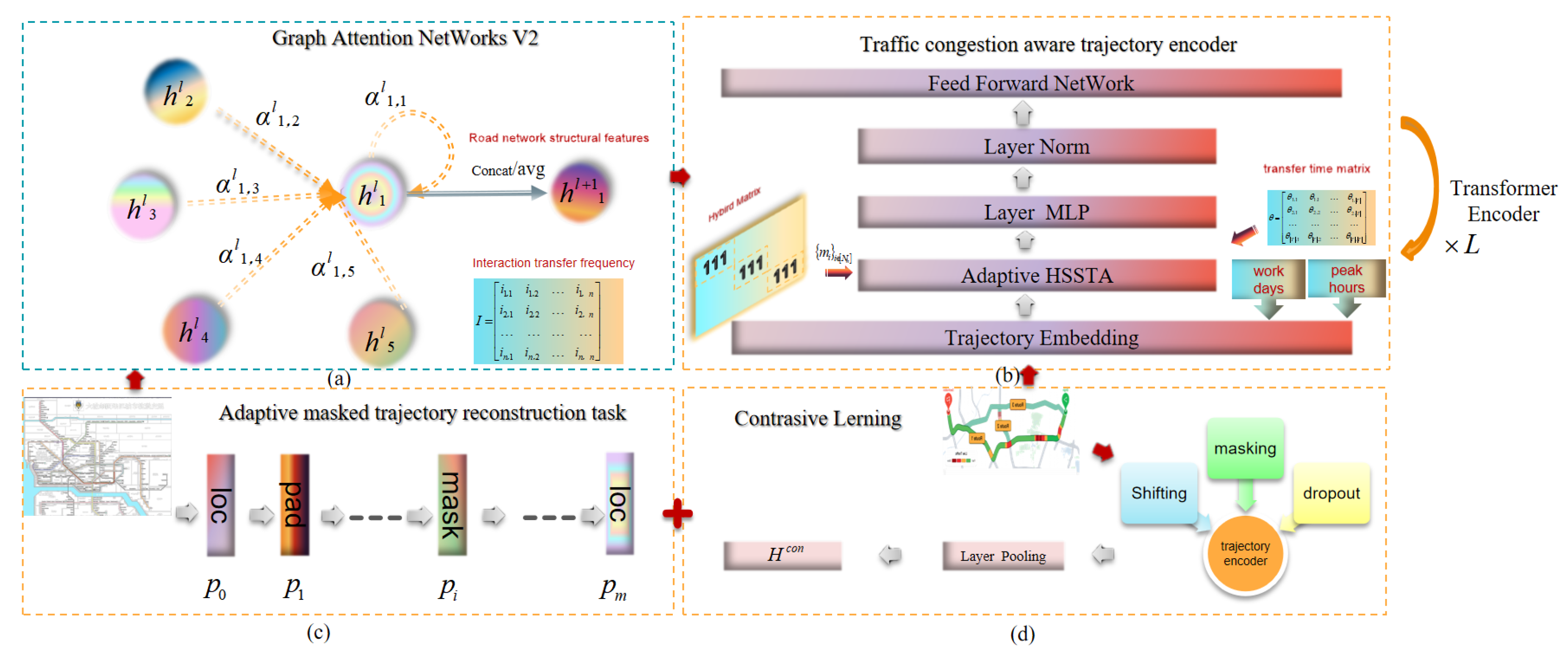
Figure 2.
The figure illustrates the process of using a hybrid matrix in the attention mechanism, where hybrid vectors are arranged in rows. Each head is assigned a dimension to enhance its expressiveness, with typically set to 64 but adjustable as needed.
Figure 2.
The figure illustrates the process of using a hybrid matrix in the attention mechanism, where hybrid vectors are arranged in rows. Each head is assigned a dimension to enhance its expressiveness, with typically set to 64 but adjustable as needed.
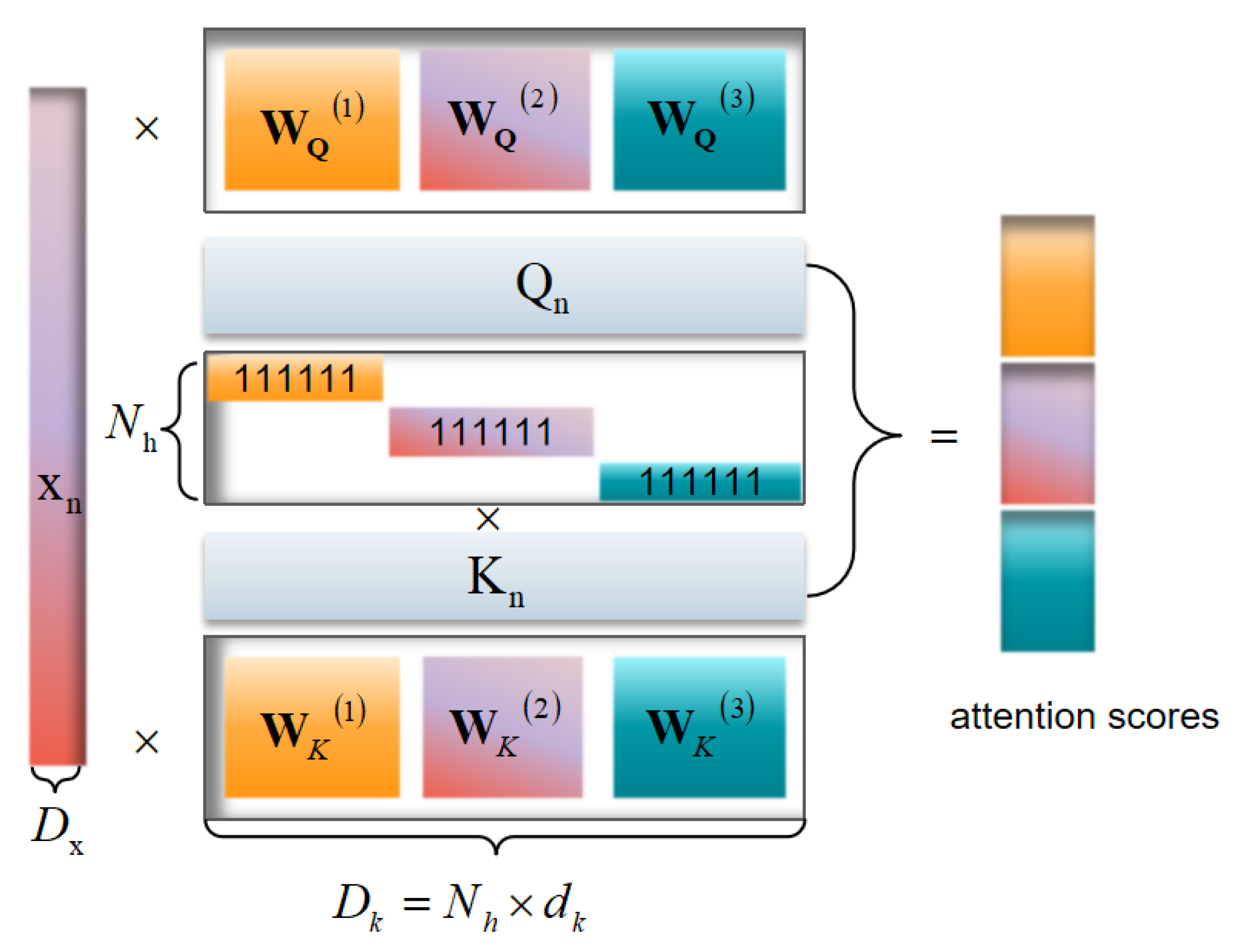
Figure 3.
The impact of Enhanced GATv2. "No-GATv2" replaces GATv2 with random embeddings, "Node2vec" uses embeddings based on road network structure, and "GAT" performs worse than GATv2 due to ignoring transition frequency variations and lower noise robustness.
Figure 3.
The impact of Enhanced GATv2. "No-GATv2" replaces GATv2 with random embeddings, "Node2vec" uses embeddings based on road network structure, and "GAT" performs worse than GATv2 due to ignoring transition frequency variations and lower noise robustness.
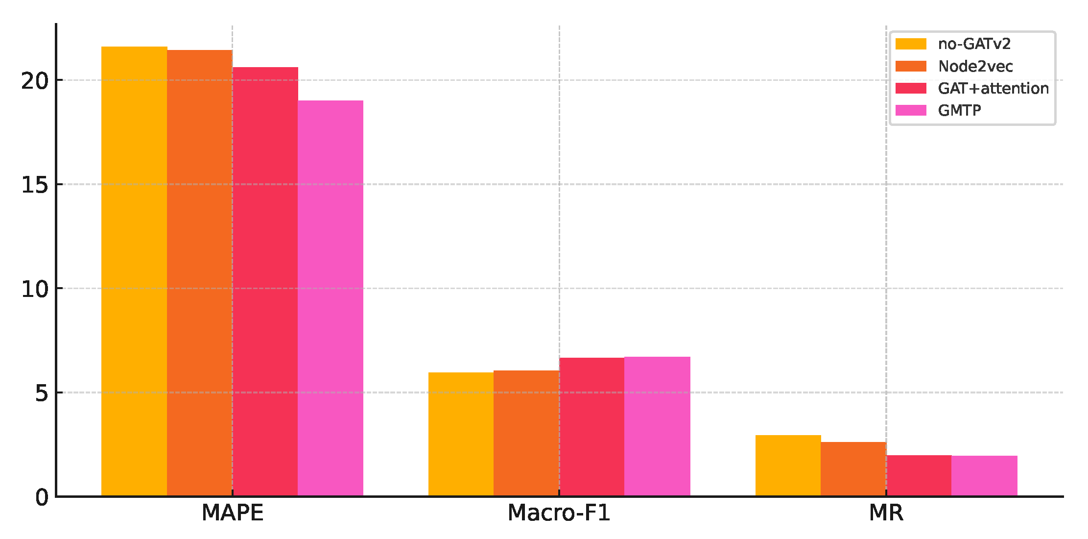
Figure 4.
The impact of Adaptive HSSTA. "No-TimeEmb" indicates the absence of time characteristics, "No-TransferMatrix" means transfer times are not considered, and "No-HybridMatrix" denotes the exclusion of the mixing matrix in attention weight calculation. Ignoring these components leads to a significant drop in model performance.
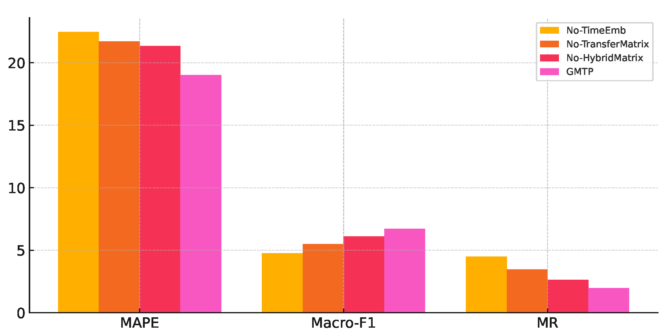
Figure 5.
Impact of self-supervised tasks.In the "No-Mask" and "No-Contra" settings, the model’s MAPE, Macro-F1, and MR values all increased, highlighting the significance of both trajectory masking and contrastive learning in self-supervised training.
Figure 5.
Impact of self-supervised tasks.In the "No-Mask" and "No-Contra" settings, the model’s MAPE, Macro-F1, and MR values all increased, highlighting the significance of both trajectory masking and contrastive learning in self-supervised training.
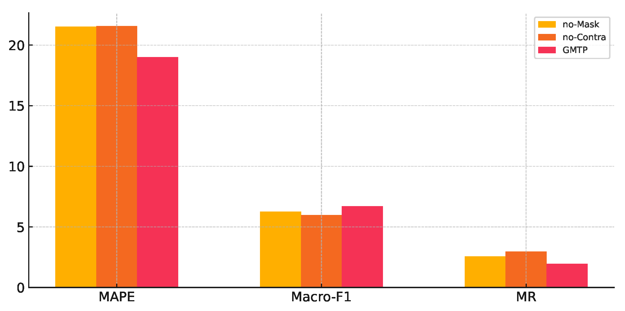
Figure 6.
Impact of data augmentation strategies. Darker colors in the heatmap represent lower MAPE values, indicating better performance. The combination of Perturb and Mask yields the best results.
Figure 6.
Impact of data augmentation strategies. Darker colors in the heatmap represent lower MAPE values, indicating better performance. The combination of Perturb and Mask yields the best results.
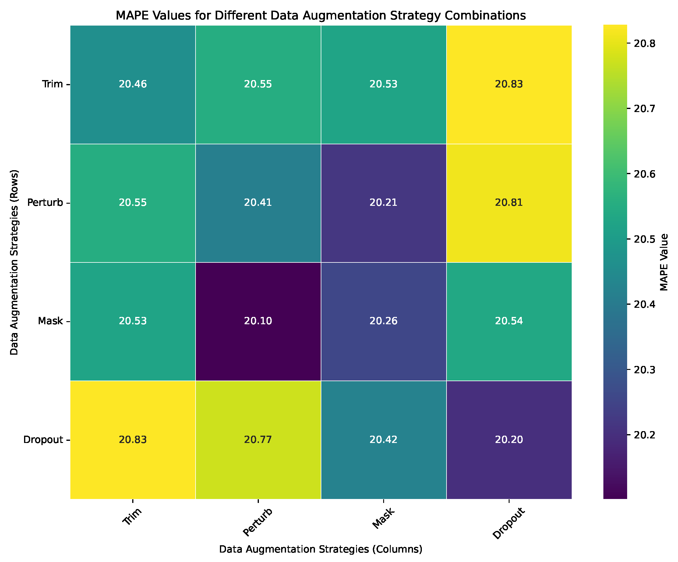
Figure 7.
The impact of hyperparameters. The vertical axis represents Macro-F1. (a) Encoding layer depth (L): Balances learning capacity and overfitting. (b) Embedding dimension (d): Affects representation quality. (c) Batch size (N): Impacts gradient estimation and contrastive learning.
Figure 7.
The impact of hyperparameters. The vertical axis represents Macro-F1. (a) Encoding layer depth (L): Balances learning capacity and overfitting. (b) Embedding dimension (d): Affects representation quality. (c) Batch size (N): Impacts gradient estimation and contrastive learning.
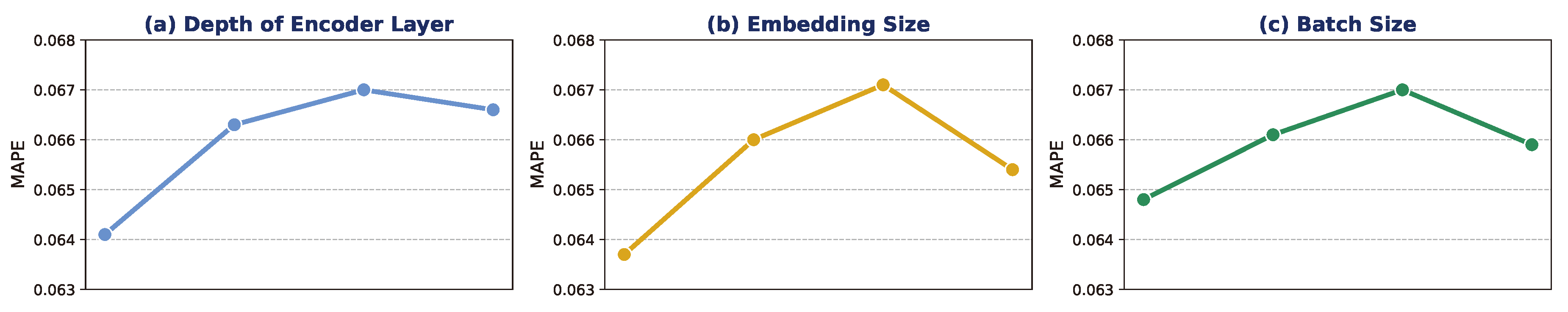
Figure 8.
Trajectory encoding time comparison. The horizontal axis represents dataset size (in K), and the vertical axis represents encoding cost (in seconds).
Figure 8.
Trajectory encoding time comparison. The horizontal axis represents dataset size (in K), and the vertical axis represents encoding cost (in seconds).
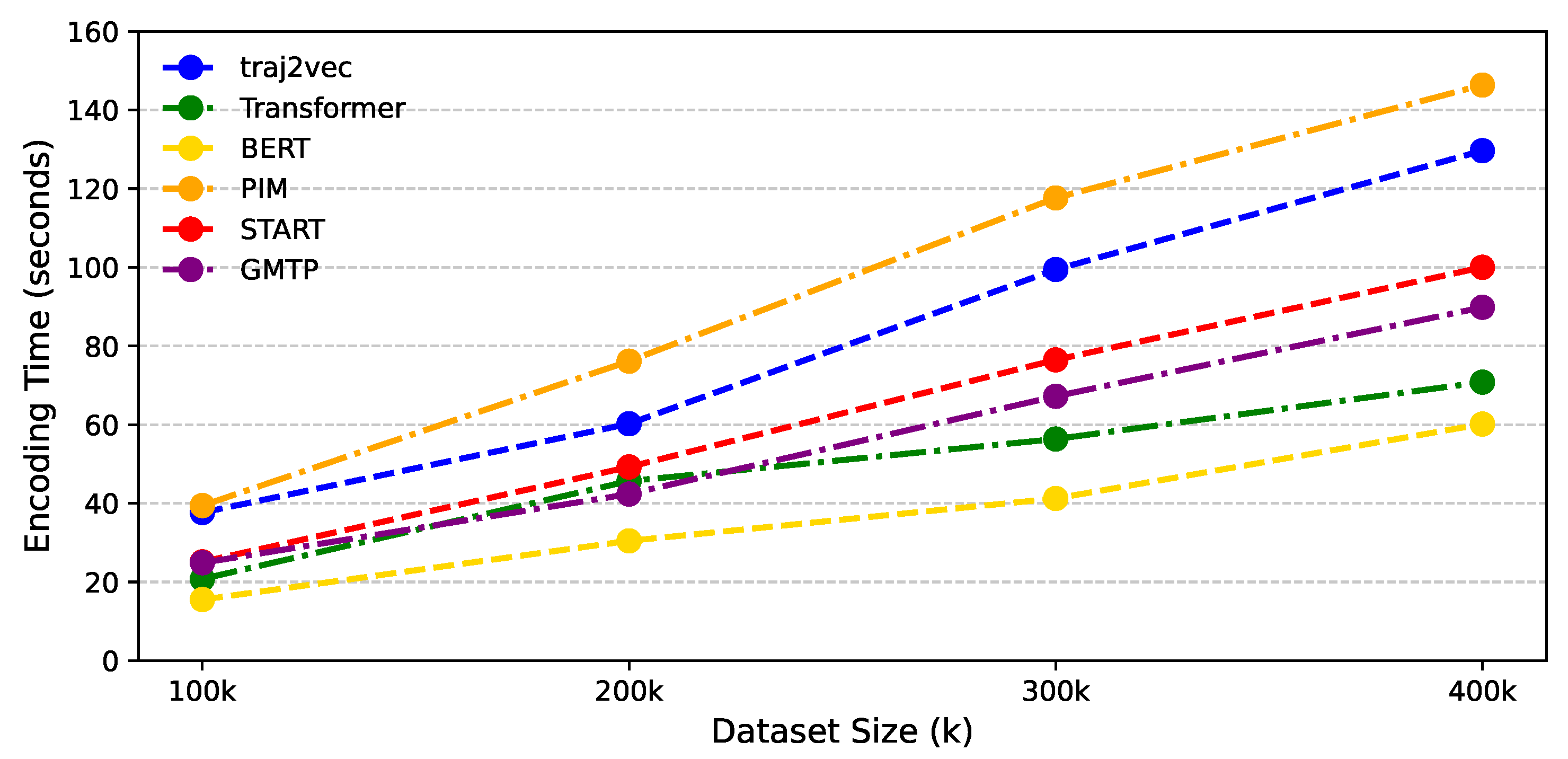

Table 1.
Dataset Description.
| Field | Description |
|---|---|
| id | Unique trajectory ID |
| path | List of road segment IDs |
| tlist | List of timestamps (UTC) |
| usr_id | User ID |
| traj_id | Original trajectory ID |
| start_time | Travel start time |
1 Note:The original trajectory dataset contains the field, with the corresponding description provided below.
Table 2.
Performance Comparison on Porto and Beijing Datasets.
| Models | Porto | Beijing | ||||
|---|---|---|---|---|---|---|
| MAE↓ | MAPE↓ | RMSE↓ | MAE↓ | MAPE↓ | RMSE↓ | |
| Traj2vec | 1.55 | 23.70 | 2.35 | 10.13 | 37.95 | 56.83 |
| Transformer | 1.74 | 25.72 | 2.64 | 10.74 | 39.61 | 57.16 |
| BERT | 1.59 | 24.63 | 2.29 | 10.21 | 37.31 | 37.31 |
| PIM | 1.56 | 24.68 | 2.34 | 10.19 | 39.04 | 57.73 |
| START | 1.33 | 20.66 | 2.00 | 9.134 | 30.92 | 35.40 |
| GMTP | 1.26 | 19.01 | 1.99 | 9.010 | 30.61 | 34.22 |
2 Note: ↓ indicates that lower values indicate better performance.
Table 3.
Comparison of Model Performance, Parameters, and Training Time Across Different Embedding Dimensions .
Table 3.
Comparison of Model Performance, Parameters, and Training Time Across Different Embedding Dimensions .
| Params () | Time (h) | |||||
|---|---|---|---|---|---|---|
| MHA | HSSTA | MHA | HSSTA | MHA | HSSTA | |
| 256 | 0.71 | 0.75 | 80.1 | 81.9 | 13.0 | 14.3 |
| 128 | 0.69 | 0.72 | 77.2 | 77.5 | 12.6 | 13.8 |
| 64 | 0.64 | 0.71 | 74.6 | 74.7 | 11.5 | 12.9 |
3 Note: MHA refers to Multi-Head Attention, and HSSTA refers to the proposed Adaptive Head Shared spatiotemporal Attention.
Disclaimer/Publisher’s Note: The statements, opinions and data contained in all publications are solely those of the individual author(s) and contributor(s) and not of MDPI and/or the editor(s). MDPI and/or the editor(s) disclaim responsibility for any injury to people or property resulting from any ideas, methods, instructions or products referred to in the content. |
© 2024 by the authors. Licensee MDPI, Basel, Switzerland. This article is an open access article distributed under the terms and conditions of the Creative Commons Attribution (CC BY) license (http://creativecommons.org/licenses/by/4.0/).
Copyright: This open access article is published under a Creative Commons CC BY 4.0 license, which permit the free download, distribution, and reuse, provided that the author and preprint are cited in any reuse.


