

Submitted:
27 November 2024
Posted:
28 November 2024
You are already at the latest version
Abstract
The estimation of complex natural frequencies in linear systems through its transient response analysis is a common practice in engineering and applied physics. In this context, the conventional Generalized Pencil of Function (GPOF) method that employs a matrix pencil of degree one, utilizing Singular Value Decomposition (SVD) filtering, has emerged as a prominent strategy to carry out a complex natural frequencies estimation. However, some modern engineering applications increasingly demand higher accuracy estimation. In this context, some intrinsic properties of Hankel matrices and exponential functions are utilized in this paper in order to develop a modified GPOF method which employs a matrix pencil of degree greater than one. Under conditions of low noise in the transient response, our method significantly enhances accuracy compared to the conventional GPOF approach. This improvement is especially valuable for applications involving closely spaced complex natural frequencies, where a precise estimation is crucial.
Keywords:
Pencil
; Prony
; resonance
; super-resolution
; accuracy
; polynomial matrix
0. Introduction
0.1. Background
The accurate representation of a system’s transient signal as a sum of damped complex harmonic functions presents a significant numerical challenge that is essential for solving various engineering and physics problems. A critical aspect of this challenge is estimating the natural complex resonance frequencies (NCRF) of the linear system under investigation. Numerous techniques have been proposed to address this issue, including the Fast Fourier Transform, Prony’s method, Total Least Squares Prony’s method, and more recently, the Generalized Pencil of Functions (GPOF) method, also known as the Matrix Pencil method. The GPOF method, introduced by Hua and Sarkar in 1989 [1], was enhanced in 1995 to improve its performance in noisy environments [2]. Due to its computational efficiency and robustness against noise [3], the GPOF method has been widely adopted for various practical applications, including power system harmonics monitoring, biomedical monitoring, remote vital sign surveying, magnetic resonance imaging, super-resolution microscopy, noninvasive blood glucose monitoring, gravitational wave detection, radar, identification of concealed firearms, military aircraft recognition, sonar, seismic data processing, meta-material design, and Coriolis mass flow meter signal processing [4,5,6,7,8,9,10,11,12,13,14,15,16,17,18,19,20,21]. In the geosciences and remote sensing fields, the GPOF method has proven useful for tasks such as localization and identification of buried objects, soil characterization, and topographic studies through radar techniques [22,23,24].
In this context, some applications may demand greater precision than the conventional GPOF algorithm can offer in order to extract valuable information from transient signals. This is particularly relevant for engineering challenges associated with radar and spectroscopy system design, as well as image super-resolution processing in medical imaging, microscopy, and astronomy [25,26,27,28].
In scenarios where applications require the discrimination of closely spaced complex natural frequencies, it may be also necessary to employ a more precise algorithm. An example of this is found in super-resolution microscopy, where very similar complex natural frequencies need to be estimated [11].
Conventionally, the GPOF method utilizes a linear matrix pencil, which involves a polynomial matrix of degree one [1,2]. In this work, we develop a GPOF method based on a polynomial matrix pencil of degree greater than one. We demonstrate that this new nonlinear GPOF approach can enhance computational accuracy for applications requiring improved precision, provided that the transient response of the system is measured and sampled with low noise levels.
0.2. Conventional Generalized Pencil of Function (GPOF) Method Revisited
Let a signal that represents the transient response of a linear system, which can be expressed as a sum of damped complex harmonics plus noise :
Then, the data set is generated by means of an uniform sampling of , as follows:
where is the sampling interval, N is the number of complex natural resonance frequencies (CNRFs) or poles, is the system NCRF, is the complex residue, and is the discrete complex pole. Here, M is the total number of samples, and m is an integer such that . It is important to note that represents the damping factor of the harmonic, while corresponds to the natural oscillation frequency of resonance for that harmonic.
Next, we highlight some fundamental aspects of the linear algebra associated with the conventional GPOF method. A matrix pencil of degree is defined as a polynomial function of the form:
where the polynomial coefficients are real rectangular matrices and is a positive integer. Here, is a complex scalar [29]. The conventional linear GPOF method is derived from a matrix pencil function of degree :
where and are Hankel matrices containing samples from the transient response . The objective of this approach is to solve the generalized eigenvalue problem:
where each computed value of corresponds to each one of the N possible complex eigenvalue-eigenvector pairs represented by , for [1].
1. Proposed Generalized Pencil of Function Method with an Increased Matrix Polynomial Degree
1.1. Definitions
In this work, we propose a matrix pencil polynomial of the form
where is a positive integer. This leads to the solution of a generalized nonlinear eigenvalue problem given by
which is aimed at determining the complex natural frequencies of the linear system under study from its transient response . To achieve this, we follow a procedure analogous to the conventional linear matrix pencil method.
First, we organize the data samples appropriately. A new Hankel matrix, denoted as , is defined with dimensions :
This matrix includes the entire dataset , where L is a positive integer known as the pencil parameter, satisfying the condition . Additionally, the column of is represented by the vector , defined as
for , where the superscript H denotes the conjugate transpose. Thus, the Hankel matrix can be expressed as
To implement the proposed method, we need to construct a generic matrix by extracting columns from . The proposed structure for is given by
for . We also define a set of Hankel matrices derived from Eq. (11):
Some specific elements of this set can be represented as follows:
It is worth highlighting that comprises the first L columns of the matrix and that comprises the last L columns of the matrix .
1.2. Properties of the Hankel Matrices Set
In this section, we leverage certain intrinsic properties of uniformly sampled transient exponential signals and Hankel matrices in order to propose some expressions that are useful to develop the proposed method. As in [1], it is convenient to write that
where the matrices , , , , and are defined as follows:
Next, we define as the Moore-Penrose pseudo-inverse of . A relationship between and can then be established from Eqs. (18) and (19):
Note that in Eq. (13) consists of the first L columns of the matrix . Moreover, due to the properties of Hankel matrices, can be constructed by eliminating the first column of (denoted as ) and appending the column as the last column. This implies that, relative to , is shifted by one column compared to . Consequently, each element of the matrix is shifted by one sampling interval compared to its corresponding element in .
Similarly, it can be inferred from Eqs. (14) and (15) that is also shifted by one column with respect to . Therefore, by induction, the relationship between and mirrors that between and . Hence, we can express:
Then, a generalized relationship can be derived between and :
1.3. Defining the Eigenvalue Problem
Since the diagonal matrix contains the values of to be determined, it is important to note that the product , derived from Eq. (30) and the inversion of Eq. (18), can be expressed as
where is a diagonal matrix containing the eigenvalues of . Consequently, Eq. (31) can also be reformulated as
This leads us to define a new generalized eigenvalue problem as follows:
where each represents the eigenvalues of the linear system to be computed, and denotes their associated eigenvectors. Notably, if , the expression in parentheses in Eq. (33) assumes the form of the matrix pencil of degree defined in Eq. (6).
Furthermore, if we left-multiply Eq. (33) by and set , denoting , we can express it as
where is an identity matrix.
1.4. Computing the Values of the Complex Natural Frequencies
In this work, the eigenvalue problem defined in Eq. (34) is not solved directly. Instead, to mitigate the adverse effects of noise present in , we decompose the matrix using its singular value decomposition (SVD) as described in [2]:
where H denotes the conjugate transpose operator, and is a diagonal matrix whose diagonal elements, denoted as , are the singular values of for . These singular values are organized in in descending order, such that .
Next, we compute the ratios for , and define a truncation criterion as follows:
where T is an integer satisfying , and p represents the number of significant decimal digits in the data.
We then define truncated versions of the matrices , , and as , , and , respectively. The matrices and are formed by taking the first T columns of and , while consists of the first T rows and columns of [2].
To filter out noise, we obtain a less noisy but approximate matrix as follows:
Following a similar methodology to that outlined in [2], which enhances the accuracy of the GPOF method in noisy environments, both matrices and must retain L columns.
Thus, we can express the singular value decompositions of and as follows:
where is constructed by retaining the first L rows of , and is formed from the last L rows of .
From Eqs. (34), (38), and (39), we can then define and solve the following eigenvalue problem computationally:
Letting represent the eigenvalues of for , we note that there are multiple possible solutions for any . Since with , and for any integer , the multiplicity of possible values for and the imaginary part of can be established by rewriting the equality as follows:
While , as given by Eq. (42), is unique, , as given by Eq. (43), is not, warranting further investigation. According to the Nyquist sampling criterion, , constraining all possible values of to the interval:
Thus, , , and are functions of the integer variable . This solution multiplicity is intrinsic to any matrix pencil polynomial of degree . Designating that is the true value among the set of possibilities of , it is useful to define the scalar as the absolute value of the determinant of the matrix pencil expressed in Eq. (34), evaluated for (the conventional linear case):
According to linear algebra theory, in the absence of noise, a true complex natural frequency and its related eigenvalue yield .
In practical cases, however, noise is always present in the signal . Thus, the correct solution for and is found at , where belongs to the set of integer values defined by the restriction (44). The value must minimize the function (see Figure 1). Consequently, the appropriate values of , , and , which characterize the studied signal , can be estimated. This process must be repeated to determine each one of the N values of , , and , since .
If necessary, the residues of the signal can also be estimated as the diagonal elements of the matrix obtained from Eq. (18):
In this way, the analytic approach to the system transient signal defined in Eq. (1) is finally established.
1.5. Relation Between the Proposed Method and the Conventional GPOF Method
The well-known conventional GPOF method is a specific case of the previously proposed method, obtained by setting the pencil degree to one (). To illustrate this, we can evaluate the matrices , , , , and at . The matrix given by Eq. (8) then takes the form:
which corresponds to the Hankel matrix proposed in [1]. Similarly, the matrix set defined in Eq. (12) for consists of only two matrices, and , which are the same as those defined for the conventional GPOF method in [1]. Furthermore, for , the auxiliary matrices and presented in Eqs. (21) and (22) become equal to the matrices and , respectively, both of which are also defined for the conventional GPOF method in [1]:
1.6. Analytical Estimation of the Variation in Complex Natural Frequencies
We now present a first-order approximation of the numerical error incurred when computing the complex natural frequency using the proposed method (Eq. (6)) compared to the conventional method (Eq. (5)). First, given that , we can establish:
where is the first-order differential operator, and represents the error associated with the proposed algorithm in computing from .
Notably, for the particular case of , we have:
where indicates the perturbation in when it is computed using the conventional GPOF method, resulting from the propagation of error in [1].
A relationship between both errors can be established as follows. First, observe that the conventional algorithm with SVD decomposition estimates the values of numerically as the eigenvalues of the matrix (Eq. (40) for ). Second, the proposed algorithm estimates from the eigenvalues of the matrix (Eq. (40) for ) in a similar manner. Thus, the precision of the estimate of appears to be of the same order as that of . Consequently, the absolute errors for both estimates can be approximated as:
This leads to the ratio of errors and being approximated as:
Under the condition that , which can typically be achieved by selecting a sufficiently small sampling period such that implies , we can define an Improvement Accuracy Ratio (IAR) as follows:
From Eq. (54), we observe that the IAR decreases as the polynomial matrix degree increases, suggesting that the precision of the proposed method may surpass that of the conventional method, since .
2. Results
To investigate the performance of the proposed method, we designed and conducted four experiments. The first three experiments utilized single precision numeric format, while the fourth employed a double precision one.
For this study, we used an artificial test transient signal defined as follows:
where represents additive Gaussian white noise. The complex natural frequencies to be estimated are defined as , , , , , , , and .
The details of these experiments are presented in Sections 3.1, 3.2, 3.3, and 3.4 below.
2.1. A First Comparison of Accuracy from Proposed and Conventional Methods
In this first case study, the parameters of the signal were defined as follows: , , ; , , ; , , ; and , , . The number of elements N on the diagonal of the matrix , the pencil parameter L, the pencil order , and the truncation factor T were set to , , , and , respectively.
The signal was sampled from to with a sampling frequency of , corresponding to a sampling time of and samples.
Additionally, was contaminated with noise to achieve a signal-to-noise ratio (SNR) of 150 dB. The errors were defined as follows:
where , , and represent the estimated values of , , and , respectively.
Finally, the errors were computed for both algorithms. Figure 2 illustrates the resulting errors from the proposed method (for ) and the conventional GPOF method, plotted in the complex plane for an SNR of 150 dB.
2.2. Average Accuracy from the Proposed and Conventional Methods in Presence of Different Levels of Noise
In this case study, the parameters of the signal were defined as follows: , , ; , , ; , , ; and , , . The number of elements N on the diagonal of the matrix , the pencil parameter L, the pencil order , and the truncation factor T were set to , , , and , respectively.
The signal was sampled from to with a sampling frequency of , resulting in a sampling time of and samples.
Both methods were then applied to realizations of in the presence of noise, over 24 different values of SNR, ranging from 30 dB to 170 dB. From the estimated values (i.e., and ), the root mean square errors and were calculated for all SNRs as follows:
where and denote the estimated values of and for any algorithm in the realization.
2.3. Accuracy from the Proposed Method as a Function of Different Pencil Degrees
In this case study, the parameters of the signal were set as follows: , , , and . The number of elements N on the diagonal of the matrix , the pencil parameter L, and the truncation factor T were set to , , and , respectively. The signal was sampled from to with a sampling frequency of , corresponding to a sampling time of and samples.
Both methods were then applied to realizations of in the presence of noise with a signal-to-noise ratio (SNR) of 125 dB, for 20 distinct values of , in the range comprised from to .
An average error in the estimates of from both methods was defined as:
where denotes the estimated value for the realization. Subsequently, this mean error was computed using Eq. (59). The mean error values were later used to compute the estimated improvement accuracy ratio (IAR) as follows:
2.4. A Comparison Between the Accuracy of the Proposed Method and the Conventional One When the Values of Complex Natural Frequencies Are Close to Each Other
Finally, we examine the performance of both the proposed and conventional algorithms applied to a signal where the complex natural frequencies are very close to each other.
In this case study, the signal consists of three damped harmonic functions characterized by the following parameters: , , , , , , , , , and . No Gaussian noise was added to in this instance, meaning only numerical noise is present. The number of elements N on the diagonal of the matrix , the pencil parameter L, the pencil degree , and the truncation factor T were set to , , , and , respectively. The signal was sampled from to with a sampling frequency of , corresponding to a sampling time of and samples.
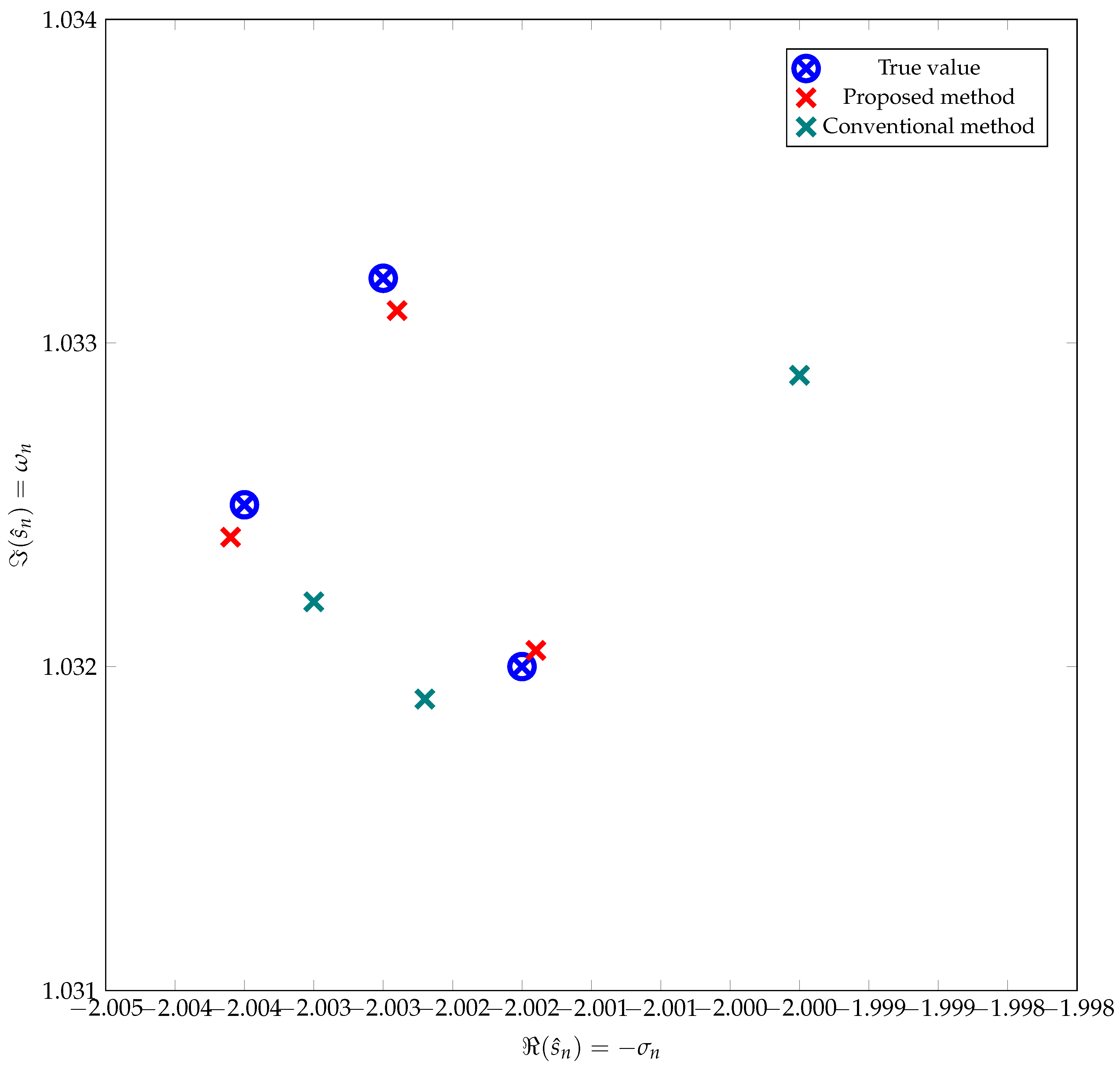
The estimations of , , and from both methods for one realization are plotted in Figure 6.
3. Discussion
Based on the results presented above, the proposed method accurately calculates the complex natural frequencies of the system from a given transient response . Furthermore, it demonstrates greater accuracy than the conventional linear method, particularly in the presence of low noise levels. Figure 2, Figure 3 and Figure 4 illustrate that the proposed method yields lower estimation errors for compared to the conventional method when the signal-to-noise ratio (SNR) exceeds 100 dB, especially when using single-precision numeric format. However, for SNRs below 100 dB, the precision of the proposed method becomes comparable to that of the conventional method (see Figure 3 and Figure 4).
The improvement in precision of the proposed method under low noise conditions becomes increasingly evident as rises, as shown in Figure 5. The improvement factor indicates that the estimation error for decreases if increases. A good agreement between numerically and analytically estimated IAR values is observed in Figure 5.
Another notable advantage of the proposed method is its performance when analyzing transient signals with closely spaced complex natural frequencies. When employing double precision and considering only numerical noise, the estimated values obtained using the proposed method are significantly more precise than those derived from the conventional matrix pencil method, as illustrated in Figure 6.
4. Conclusion
In this work, we propose a nonlinear matrix pencil method with a pencil degree , such as , in order to estimate the natural complex frequencies of resonance in a given linear system. The proposed method has been thoroughly investigated and compared with the conventional GPOF method.
An analytical approximation for the estimation error of these complex frequencies was developed and validated through simulations. The results demonstrate that the proposed method not only accurately estimates the complex natural frequencies of the system but also achieves higher precision under low noise condition compared to the GPOF method. Specifically, when using single precision, the improvement in accuracy is observed for signal-to-noise ratios (SNR) greater than 100 dB, and this enhancement becomes more pronounced as the nonlinear pencil degree increases.
Moreover, the findings indicate that the proposed method is particularly effective in estimating complex natural frequencies when they are closely spaced under low noise condition.
Author Contributions
Conceptualization, R.B.S.; methodology, R.B.S. and A.J.Z.; software, R.B.S. and A.J.Z.; validation, R.B.S.; investigation, R.B.S. and A.J.Z.; resources, A.J.Z.; writing—original draft preparation, R.B.S. and A.J.Z.; writing—review and editing, R.B.S. and A.J.Z.; visualization, R.B.S. and A.J.Z.; supervision, A.J.Z.; project administration, A.J.Z. All authors have read and agreed to the published version of the manuscript.
Funding
Project funded by the Research Continuity Project Fund, year 2022, code LCLI22-02, Universidad Tecnológica Metropolitana.
Data Availability Statement
The data will be made available by the authors on request.
Acknowledgments
The authors would like to thank Chat GPT for its assistance in proofreading and editing this manuscript. The AI tool helped identify and correct errors in grammar, spelling, and punctuation. However, the authors also conducted a thorough manual review to ensure the accuracy and clarity of the content.
Conflicts of Interest
The authors declare no conflicts of interest. The funders had no role in the design of the study; in the collection, analyses, or interpretation of data; in the writing of the manuscript; or in the decision to publish the results.
Abbreviations
The following abbreviations are used in this manuscript:
| NCRF | Natural Complex Resonance Frequencies |
| GPOF | Generalized Pencil of Function |
| SVD | Singular Value Decomposition |
| IAR | Improvement Accuracy Ratio |
References
- Hua, Y.; Sarkar, T.K. Generalized pencil-of-function method for extracting poles of an EM system from its transient response. IEEE Transactions on Antennas and Propagation 1989, 37, 229–234. [Google Scholar] [CrossRef]
- Sarkar, T.K.; Pereira, O. Using the matrix pencil method to estimate the parameters of a sum of complex exponentials. IEEE Antennas and Propagation Magazine 1995, 37, 48–55. [Google Scholar] [CrossRef]
- Barroso, R.; Zozaya, A. Prony’s method and matrix pencil method performance on determining the complex natural resonance frequencies of a linear system. Revista Internacional de Métodos Numéricos para Cálculo y Diseño en Ingeniería 2022, 38. [Google Scholar] [CrossRef]
- Crow, M.L.; Singh, A. The Matrix Pencil for Power System Modal Extraction. IEEE Transactions on Power Systems 2005, 20, 501–502. [Google Scholar] [CrossRef]
- Yang, L.; Jiao, Z.; Kang, X.; Wang, X. A Novel Matrix Pencil Method for Real-time Power Frequency Phasor Estimation under Power System Transients. In Proceedings of the 12th IET International Conference on Developments in Power System Protection, Copenhagen, Denmark, 31 March 2014. [Google Scholar]
- Hossein, Q.; Hojiat, A. A comparative study of signal processing methods for structural health monitoring. Journal of Vibroengineering 2016, 18, 2186–2204. [Google Scholar]
- Chamaani, H.M.; Akbarpour, A.; Helbig, M.; Sachs, J. Matrix pencil method for vital sign detection from signals acquired by microwave sensors. Sensors 2021, 21, 5735. [Google Scholar] [CrossRef] [PubMed]
- Fricke, S.N.; Seymour, J.D.; Battistel, M.D.; Freedberg, D.I.; Eads, C.D.; Augustine, M.P. Data processing in NMR relaxometry using the matrix pencil. Journal of Magnetic Resonance 2020, 313, 106704. [Google Scholar] [CrossRef] [PubMed]
- Bauman, G.; Bieri, O. Matrix pencil decomposition of time-resolved proton MRI for robust and improved assessment of pulmonary ventilation and perfusion. Magnetic Resonance in Medicine 2016, 77, 336–342. [Google Scholar] [CrossRef] [PubMed]
- Wang, Y.; Lee, H.; Apte, D. Quantitative NMR Spectroscopy by Matrix Pencil Methods. International Journal of Imaging Systems and Technology 1992, 4, 201–206. [Google Scholar] [CrossRef]
- Ehler, M.; Kunis, S.; Peter, T.; Richter, C. A randomized multivariate matrix pencil method for superresolution microscopy. Electronic Transactions on Numerical Analysis 2019, 51, 63–74. [Google Scholar] [CrossRef]
- Li, Q.; Xiao, X.; Kikkawa, T. Noninvasive Blood Glucose Level Detection Based on Matrix Pencil Method and Artificial Neural Network. Journal of Electrical Engineering and Technology 2021, 16, 2093–7423. [Google Scholar] [CrossRef]
- Li, M.; Li, S.; Yu, Y.; Ni, X.; Chen, R. Design of random and sparse metalens with matrix pencil method. Optics Express 2018, 26, 24702–24711. [Google Scholar] [CrossRef] [PubMed]
- Kokkinos, T.; Adve, R.S.; Sarris, C.D. Spectral analysis of negative refractive index metamaterials utilizing signal processing techniques and time-domain simulations. In Proceedings of the IEEE/ACES International Conference on Wireless Communications and Applied Computational Electromagnetics, Honolulu, USA, 03-07 April 2005. [Google Scholar]
- Adve, R. Defence Research Reports. Target Identification using Matrix Pencil. Available online: https://pubs.drdc-rddc.gc.ca/BASIS/pcandid/www/engpub/SF.
- Sabio, V. Defense Technical Information Center. Target recognition in ultra-wideband sar imagery. Available online: https://apps.dtic.mil/sti/tr/pdf/ADA283462.pdf (accessed on 01 January 2024).
- Berti, E.; Cardoso, V.; Gonzalez, J.; Sperhake, U. Mining information from binary black hole mergers: A comparison of estimation methods for complex exponentials in noise. Physical Review D 2007, 75. [Google Scholar] [CrossRef]
- Drissi, K.; Poljak, D. The Matrix Pencil method applied to smart monitoring and radar. In Proceedings of the 17th International Conference on Computational Methods and Experimental Measurements, 5-7 May 2015. [Google Scholar]
- Harmer, S.W.; Andrews, D.A.; Rezgui, N.D.; Bowring, N.J. Detection of handguns by their complex natural resonant frequencies. IET Microwaves Antennas and Propagation 2010, 4, 1182–1190. [Google Scholar] [CrossRef]
- Persichkin, A.; Shpilevoy, A. About the method of estimating the parameters of seismic signals. IKBFU´s Herald. Ser. Physics, Mathematics and Technology 2015, 10, 122–125. [Google Scholar]
- Li, M.; Henry, M. Signal Processing Methods for Coriolis Mass Flow Metering in Two-Phase Flow Conditions. In Proceedings of the 2016 IEEE International Conference on Industrial Technology (ICIT), Taipei, Taiwan, 14-17 March 2016. [Google Scholar]
- Rommel, T.; Huber, S.; Younis, M.; Chandra, M. Matriz pencil method for topography adaptive digital beamforming in synthetic aperture radar. IET Radar, Sonar & Navigation 2021, 1–14. [Google Scholar]
- Yochanang, C.; Boonpoonga, A.; Burintramart, S. Analysis of object buried in soil by using matrix pencil method. In 2014 International Electrical Engineering Congress (iEECON), Pattaya, Thailand, 19 - 21 March 2014.
- Chantasen, N.; Boonpoonga, A.; Athikulwongse, K.; Kaemarungsi, K.; Akkaraekthalin, P. Mapping the physical and dielectric properties of layered soil using short-time matrix pencil method-based ground penetrating radar. IEEE Access 2020, 8, 105610–105621. [Google Scholar] [CrossRef]
- Aubel, C. Performance of super-resolution methods in parameter estimation and system identification. Doctoral thesis, ETH Zurich, Switzerland, 2016.
- Bajwa, W.U.; Gedalyahu, K.; Eldar, Y. C. Identification of parametric underspread linear systems and super-resolution radar. IEEE Transactions on Signal Processing 2011, 59, 2548–2561. [Google Scholar] [CrossRef]
- Heckel, R.; Morgenshtern, V. I.; Soltanolkotabi, M. Super-resolution radar. Information and Inference. A Journal of the IMA , 2016, 5, 22–75. [Google Scholar] [CrossRef]
- Li, Z.; Peng, Q.; Bhanu, B.; Zhang, Q.; He, H. Super resolution for astronomical observations. Astrophysics and Space Science , 2018, 363. [Google Scholar] [CrossRef]
- Hazewinkel, M. Handbook of Algebra, 1st ed.; Elsevier, 1995; pp. 99–100.
Figure 1.
Relative locations of multiple complex natural frequency candidates with respect to the correct one in the complex plane for a noisy single-pole signal.
Figure 1.
Relative locations of multiple complex natural frequency candidates with respect to the correct one in the complex plane for a noisy single-pole signal.
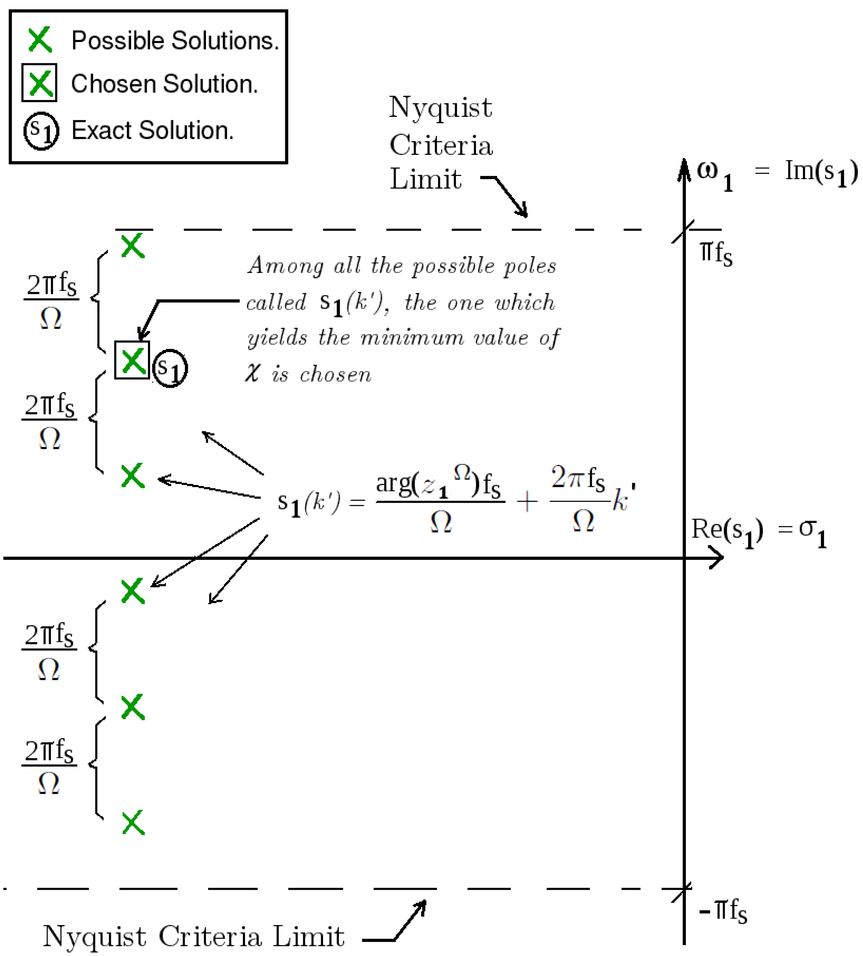
Figure 2.
Errors obtained from the proposed method (for ) and the conventional GPOF method, plotted in the complex plane for an SNR of 150 dB.
Figure 2.
Errors obtained from the proposed method (for ) and the conventional GPOF method, plotted in the complex plane for an SNR of 150 dB.
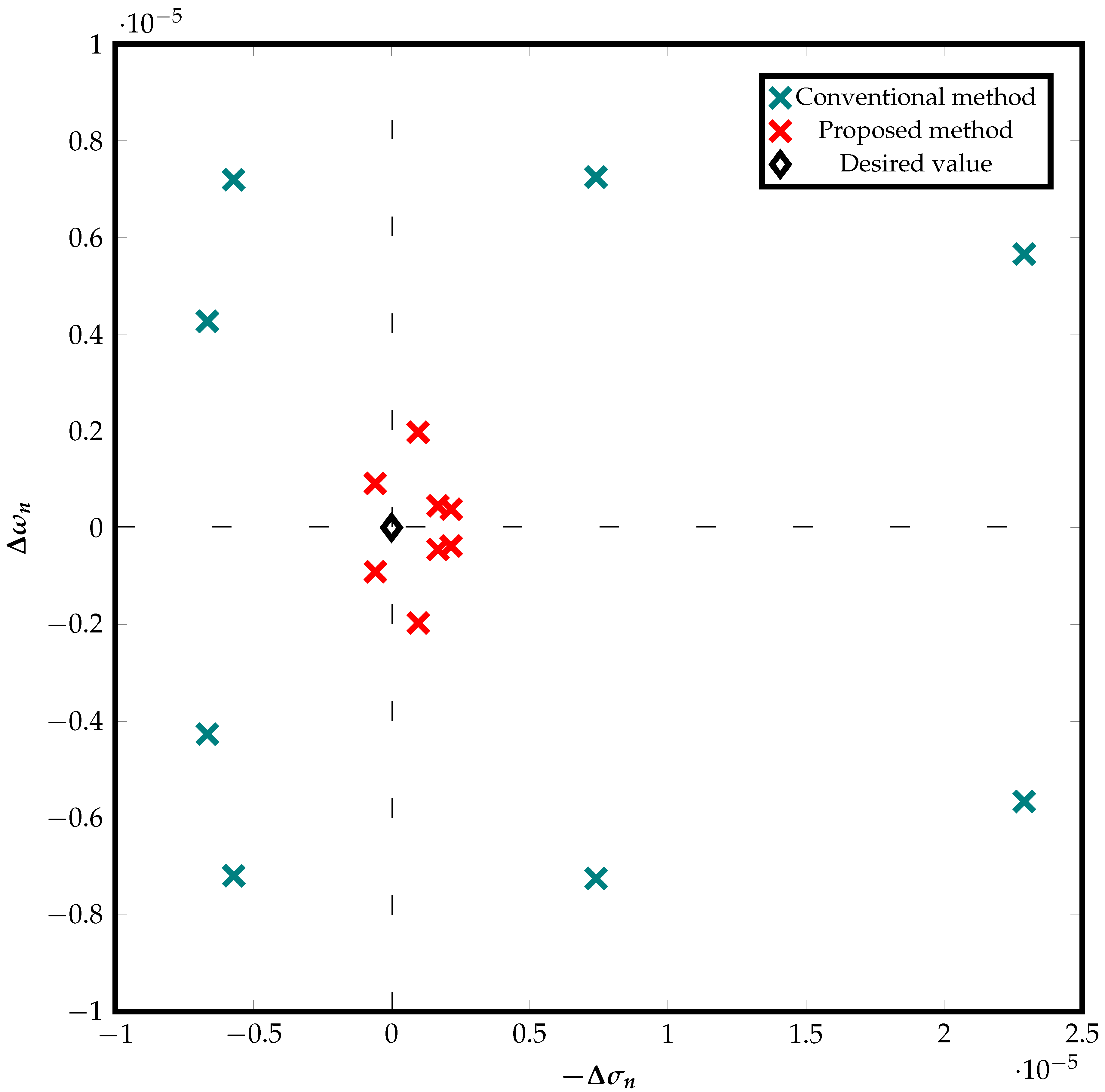
Figure 3.
Normalized mean square error (MSE) in dB for the estimate of obtained from the proposed method (for ) and the conventional GPOF method, as functions of SNR.
Figure 3.
Normalized mean square error (MSE) in dB for the estimate of obtained from the proposed method (for ) and the conventional GPOF method, as functions of SNR.
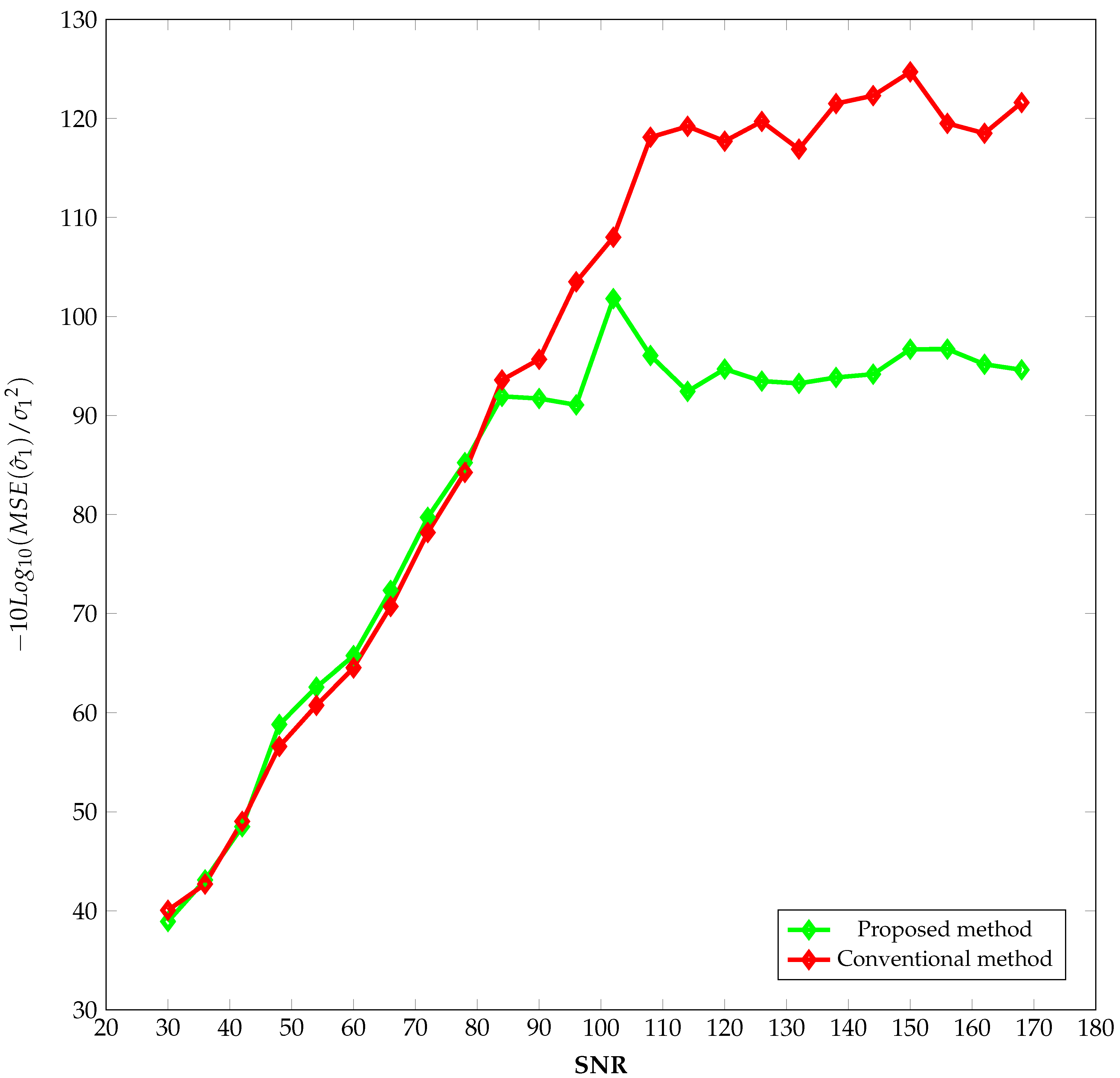
Figure 4.
Normalized mean square error (MSE) in dB for the estimate of obtained from the proposed method (for ) and the conventional GPOF method, as functions of SNR.
Figure 4.
Normalized mean square error (MSE) in dB for the estimate of obtained from the proposed method (for ) and the conventional GPOF method, as functions of SNR.
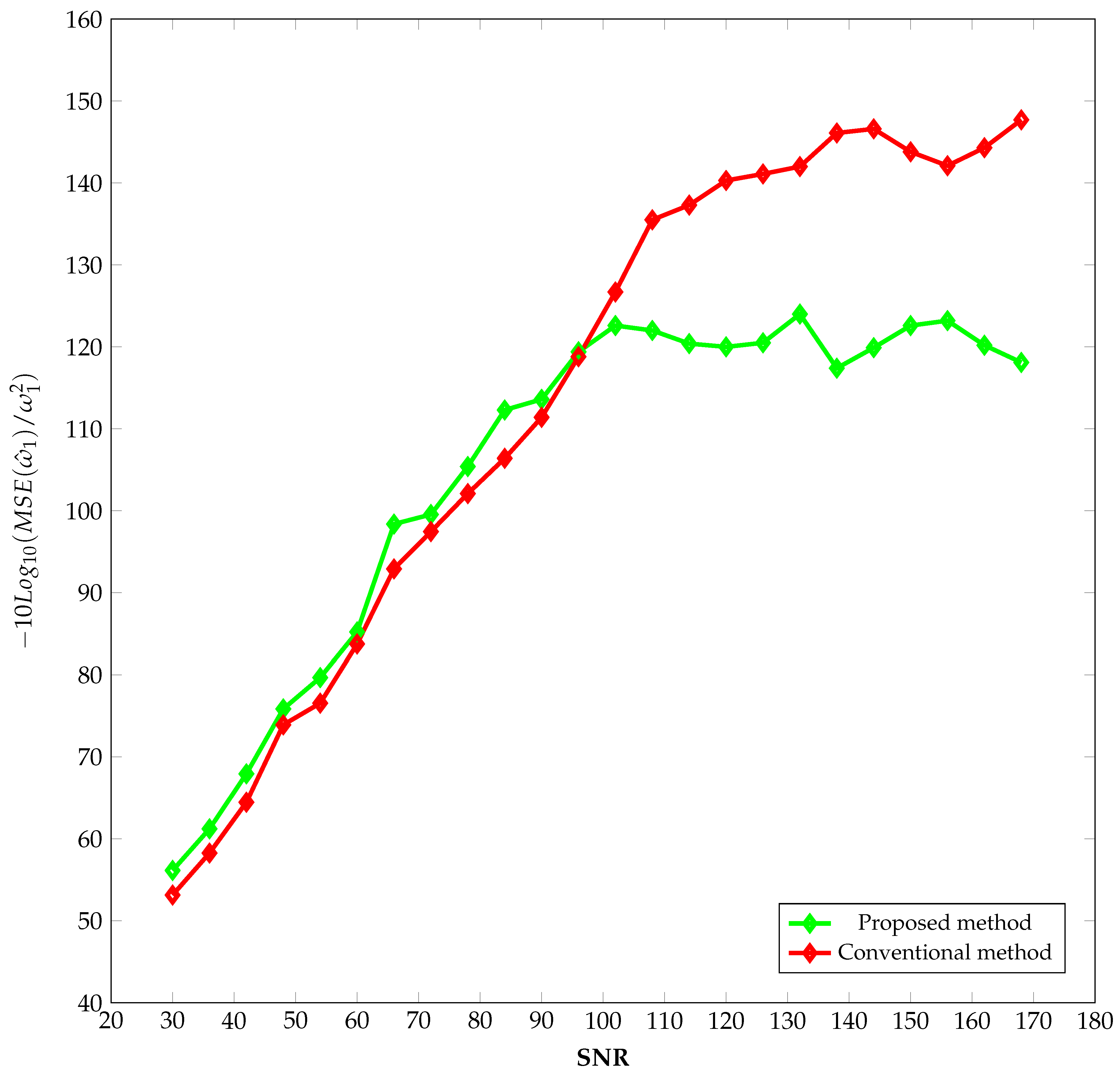
Figure 5.
Inverse values in dB of the estimated from Eq. (60) and the analytical prediction for IAR from Eq. (54), both as functions of the pencil degree .
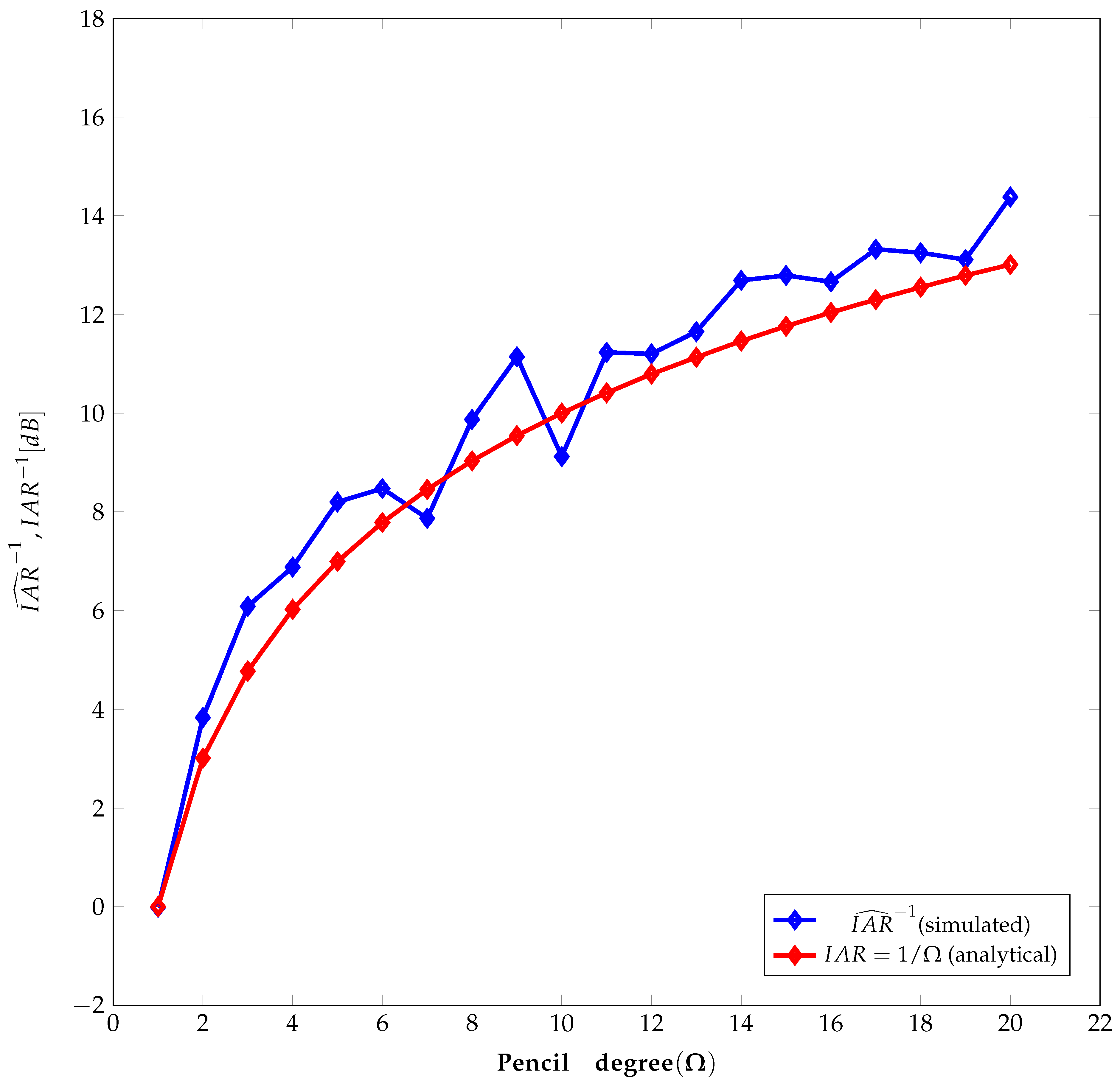
Figure 6.
Estimates of from both methods for the signal under study in the complex plane.
Short Biography of Authors
 |
Raúl Horacio Barroso Salcedo received his B.S. and his M.S.c. degrees in Electrical Engineering from the Central university of Venezuela in 2000 and 2009 respectively. Currently, he is also pursuing his P.h.D. metamaterial studies in the Faculty of Engineering of the Central University of Venezuela, and he is just a P.h.D. candidate. Since 2006 he has been a full professor in the Simon Bolivar University in Venezuela and he is currently hired there as an associated teacher. His research interests include metamaterials, fractal antennas, multiband antennas, broadband antennas, and analysis and design of broadband matching systems. Raul Barroso has published an overall of ten IEEE and IET articles as a main author in these areas. |
 |
Alfonso Zozaya received his B.Sc. degree in Electronic Engineering, with a major in Telecommunication, from the Instituto Universitario Politécnico de las Fuerzas Armadas Nacionales de Venezuela (I.U.P.F.A.N.), Maracay, Venezuela, in 1991, and his PhD degree from the Universidad Politécnica de Cataluña (UPC), Barcelona, Spain, in the area of Signal Theory and Communications in 2002. He worked as a Professor at the University of Carabobo, Valencia, Venezuela from 1994 to 2014. Currently, he is Full Professor in the Departamento de Electricidad at the Universidad Tecnológica Metropolitana (UTEM), Santiago de Chile. His research areas of interest are applied electromagnetic, computational electromagnetic, digital signal processing, RF circuits design, synthetic aperture radars, and impulsive UWB radars. |
Disclaimer/Publisher’s Note: The statements, opinions and data contained in all publications are solely those of the individual author(s) and contributor(s) and not of MDPI and/or the editor(s). MDPI and/or the editor(s) disclaim responsibility for any injury to people or property resulting from any ideas, methods, instructions or products referred to in the content. |
© 2024 by the authors. Licensee MDPI, Basel, Switzerland. This article is an open access article distributed under the terms and conditions of the Creative Commons Attribution (CC BY) license (http://creativecommons.org/licenses/by/4.0/).
Copyright: This open access article is published under a Creative Commons CC BY 4.0 license, which permit the free download, distribution, and reuse, provided that the author and preprint are cited in any reuse.