1. Introduction
The intricate relationship between genomic architecture and neural circuit differentiation has long intrigued scientists seeking to understand the foundations of neural development and function. Recent advancements in topological data analysis (TDA) have provided novel methodologies to explore this relationship, offering insights into how the topological features of genomic data influence the formation and specialization of neural circuits. By integrating concepts from differential topology and statistical mechanics, researchers can develop a comprehensive framework to elucidate the mechanisms underlying neural differentiation and functional specialization.
1.1. Topological Genomics and Neural Circuit Differentiation
Topological genomics applies principles from topology to study the organization and function of genomic data. This approach focuses on understanding how the spatial and structural properties of the genome influence biological processes (Carlsson, 2009). In the context of neural circuits, topological genomics examines how genomic features, such as chromatin loops and higher-order structures, correlate with the development and differentiation of neural networks (Edelsbrunner & Harer, 2010).
Neural circuits are complex networks of interconnected neurons that process and transmit information. The differentiation of these circuits involves the specialization of neurons and the establishment of precise connectivity patterns, which are essential for proper neural function (Bassett & Sporns, 2017). Understanding the factors that guide neural circuit differentiation is crucial for insights into neurodevelopmental processes and the etiology of neurological disorders (Fefferman, Mitter, & Narayanan, 2016).
1.2. Differential Topology in Neural Differentiation
Differential topology studies the properties of smooth manifolds and the mappings between them. In the context of neural circuits, differential topology provides tools to model the continuous transformations that occur during neural differentiation. For instance, the formation of neural circuits can be represented as a mapping from a genomic manifold to a neural manifold, capturing the transformation of genetic information into functional neural networks phenotypes (Ghrist, 2014).
Critical points in differential topology, such as cusps and folds, correspond to significant events in neural differentiation, such as the emergence of new functional regions or the reorganization of connectivity patterns. Analyzing these critical points can reveal the underlying mechanisms that drive neural circuit formation and specialization (Nakahara, 2003).
1.3. Statistical Mechanics and Energy Landscapes
Statistical mechanics provides a framework to study the behavior of systems with a large number of components, focusing on the collective properties that emerge from individual interactions (Mezard & Montanari, 2009). In neural circuits, statistical mechanics models the energy landscapes that govern the formation and stability of neural networks.
The energy landscape of a neural circuit represents the potential energy associated with different configurations of the network (Montgomery, 2024). Neural circuits tend to evolve toward configurations that minimize their energy, leading to stable and functional networks. Phase transitions in these energy landscapes correspond to significant changes in the network's structure or function, such as the differentiation of a neural circuit into a specialized functional unit (Choromanska et al., 2015).
1.4. Persistent Homology in Genomic and Neural Analysis
Persistent homology is a method in TDA that studies the multi-scale topological features of a space, capturing how features like connected components and holes appear and disappear across different scales. In genomic data, persistent homology can identify topological invariants, such as loops and voids, that correspond to functional genomic elements like enhancers and silencers (Carlsson, 2009).
In neural circuits, persistent homology can analyze the topological features of connectivity patterns, identifying structures critical for information processing. By comparing the persistent homology of genomic data with that of neural circuits, researchers can identify correlations between genomic features and neural connectivity patterns, providing insights into how genetic information influences neural circuit formation (Bassett & Sporns, 2017).
1.5. Integrating Topological Genomics, Differential Topology, and Statistical Mechanics
By integrating topological genomics, differential topology, and statistical mechanics, researchers can develop a comprehensive framework to study neural circuit differentiation. This interdisciplinary approach allows for the modeling of the transformation of genomic information into neural circuits, the analysis of the energy landscapes that govern neural differentiation, and the identification of topological features that are critical for neural function (Edelsbrunner & Harer, 2010; Mezard & Montanari, 2009).
For example, by applying persistent homology to genomic interaction maps, researchers can identify topological features that correspond to regulatory elements influencing neural differentiation. Differential topology can model how these genomic features map onto neural circuits, capturing the continuous transformations that occur during differentiation. Statistical mechanics can then model the energy landscapes associated with these transformations, identifying phase transitions that correspond to significant events in neural circuit formation (Choromanska et al., 2015).
1.6. Implications for Neurodevelopment and Neurological Disorders
Understanding the topological features of genomic data and their influence on neural circuit differentiation has significant implications for neurodevelopmental research. Aberrant topological features in genomic data, such as persistent loops or disrupted manifolds, may predict defects in neural circuit differentiation, providing insights into conditions like autism and schizophrenia (Fefferman, Mitter, & Narayanan, 2016).
Additionally, this interdisciplinary framework can inform the design of neural network architectures in artificial intelligence, improving robustness and adaptability by mimicking biological differentiation processes. Insights from topological genomics can also guide targeted genomic edits to enhance neuroplasticity or develop regenerative therapies for neurological disorders (Bassett & Sporns, 2017).
1.7. Summary
The integration of topological genomics, differential topology, and statistical mechanics offers a novel framework for understanding the relationship between genomic architecture and neural circuit differentiation. By capturing the topological invariants and energy dynamics underlying this process, researchers can gain valuable insights into neural development, function, and pathology. This interdisciplinary approach has the potential to revolutionize both theoretical neuroscience and practical applications in genomics and artificial intelligence.
2. Methodology
This methodology explores the path from genotype topology to phenotype using differential topology and manifolds, explicitly modeling how genetic and environmental differences influence phenotypic variation, including differences observed in twins. Differential topology provides the mathematical tools for analyzing the continuous transformation from genomic structure to phenotypic traits, while manifolds serve as the framework to represent the genotype and phenotype spaces.
We define the genotype and phenotype spaces as smooth manifolds:
Genotype space: , a high-dimensional manifold representing genetic variation.
Phenotype space: , a lower-dimensional manifold representing observable traits.
There exists a smooth mapping
that transforms genetic information into phenotypic traits:
- 2.
Differential Mapping and Jacobian Representation
The mapping
is differentiable, allowing us to analyze local transformations between genotype and phenotype using the Jacobian matrix:
The rank of determines the local dimensionality of the phenotype space at a given genotype point and identifies critical points where phenotypic traits change abruptly.
- 3.
Environmental Perturbations
Environmental influences are modeled as a perturbation function
, where
represents the environmental parameter space. The perturbed mapping becomes:
The environmental perturbation
is assumed to be smooth, and its effect on the genotypephenotype map can be analyzed by the modified Jacobian:
where
is the Jacobian of the environmental perturbation.
- 4.
Differences Between Twins
For monozygotic twins, the initial genotype
and
are nearly identical (
), but environmental influences
and
differ. The phenotypic difference is expressed as:
Using a first-order Taylor expansion, the phenotypic difference is approximated as:
- 5.
Critical Points and Bifurcations
Critical points in the genotype-phenotype map occur where the Jacobian
loses rank, corresponding to points of bifurcation where small genetic or environmental changes result in large phenotypic shifts:
These critical points often explain phenotypic divergence between twins despite genetic similarity.
- 6.
Genotypic Topology and Persistent Homology
To analyze the global structure of the genotype manifold
, we compute its topological invariants using persistent homology. Given a filtration
parameterized by
, we compute Betti numbers
to capture the topological features of the manifold:
where
is the
-th homology group. Persistent homology tracks how these features change across scales, providing insights into the robustness of genetic traits against environmental perturbations.
2.1. Summary of Methodology
Mapping Genotype to Phenotype: Represented as a differentiable mapping .
Environmental Effects: Incorporated as a perturbation function , modifying the genotypephenotype relationship.
Phenotypic Variability: Quantified using differential approximations of and changes in .
Critical Points: Identified via the Jacobian determinant to locate bifurcations in phenotypic traits.
Topology of Genotype Space: Analyzed through persistent homology to understand global genetic structures.
This approach bridges differential topology and environmental dynamics to mathematically characterize the genotype-to-phenotype pathway and explain variations, such as those observed in twins.
Explain twin studies using differential topology.
2.2. Explaining Twin Studies Using Differential Topology
Twin studies have historically provided invaluable insights into the interplay between genetic and environmental factors in shaping phenotypic traits. Monozygotic (MZ) twins, who share nearly identical genetic material, often exhibit phenotypic differences due to environmental influences, epigenetic changes, or stochastic developmental processes. Differential topology offers a mathematical framework to model and analyze these variations, allowing us to represent the genotype-to-phenotype map and account for differences arising from perturbations.
In differential topology, we represent the genotype and phenotype spaces as smooth manifolds:
Genotype manifold : Encodes genetic information, including variations in chromosomal regions, regulatory networks, and epigenetic states.
Phenotype manifold : Represents observable traits, such as height, cognitive abilities, or susceptibility to diseases.
The relationship between genotype and phenotype is described by a smooth map:
where
associates a genotype
to a phenotype
.
- 2.
Genetic Similarity in Twins
Monozygotic twins begin with nearly identical genetic configurations:
In this context, the genotype manifold can be viewed as a neighborhood around the shared genetic configuration of the twins. For dizygotic (DZ) twins, genetic similarity is lower, corresponding to a larger divergence within .
Differential topology allows us to analyze local properties of
using the Jacobian matrix:
The Jacobian encodes the local rate of change of phenotypic traits with respect to genetic variation. For twins, small differences in
and
lead to corresponding differences in
and
, as captured by the linear approximation:
- 3.
Environmental Perturbations
Environmental influences introduce additional variability in the phenotype manifold. Let
represent the effect of an environmental parameter
on the genotype space. The perturbed genotype-phenotype map is:
For monozygotic twins exposed to distinct environments
and
, the phenotypic difference is expressed as:
Using a first-order Taylor expansion:
where
captures the sensitivity of the genotype-phenotype map to environmental changes. This equation highlights the contributions of genetic and environmental factors to phenotypic divergence in twins.
- 4.
Critical Points and Phenotypic Divergence
Critical points in differential topology occur where the Jacobian
loses rank. These points correspond to bifurcations in the genotype-phenotype map, where small genetic or environmental differences result in large phenotypic variations. Critical points are identified by:
In the context of twins, critical points explain why certain traits (e.g., susceptibility to complex diseases) exhibit significant variability even in genetically identical individuals. Environmental factors or stochastic developmental processes may push one twin's genotype-phenotype trajectory near a critical point, leading to divergent outcomes.
- 5.
Persistent Homology of Genotype Space
To analyze the global structure of the genotype manifold, we compute its topological features using persistent homology. This method captures how genetic variations and environmental perturbations influence the robustness of traits. For the genotype manifold
, a filtration
parameterized by
is constructed, and Betti numbers
are computed:
where
is the
-th homology group. Persistent homology reveals the stability of genetic structures, identifying features that are resistant to environmental perturbations and those prone to divergence.
- 6.
Phenotypic Plasticity and Twin Differences
Phenotypic plasticity, or the ability of an organism to exhibit different traits under varying environmental conditions, is inherently topological. In twins, phenotypic plasticity can be modeled by examining how the environmental perturbation deforms the genotype manifold and its mapping . The magnitude of deformation is quantified by changes in the persistent homology of and the stability of critical points in .
For monozygotic twins, phenotypic plasticity explains why shared traits (e.g., height or facial structure) exhibit less variation, while environmentally sensitive traits (e.g., behavior or health outcomes) show greater divergence.
2.3. Summary
Differential topology provides a rigorous mathematical framework to analyze the genotype-to-phenotype map and explain variations in twin studies. By modeling genotype and phenotype as manifolds and incorporating environmental perturbations, we capture the dynamic and nonlinear processes underlying phenotypic differences. Persistent homology and critical point analysis further illuminate the mechanisms of phenotypic divergence, offering insights into the interplay of genetics
Differential topology provides a rigorous mathematical framework to analyze the genotype-to-phenotype map and explain variations in twin studies. By modeling genotype and phenotype as manifolds and incorporating environmental perturbations, we capture the dynamic and nonlinear processes underlying phenotypic differences. Persistent homology and critical point analysis further illuminate the mechanisms of phenotypic divergence, offering insights into the interaction of genetics and environment in shaping complex traits. This approach enhances our understanding of twin studies, providing a deeper theoretical basis for exploring heritability and environmental influence.
3. Results
3.1. Explanation of the Graphs
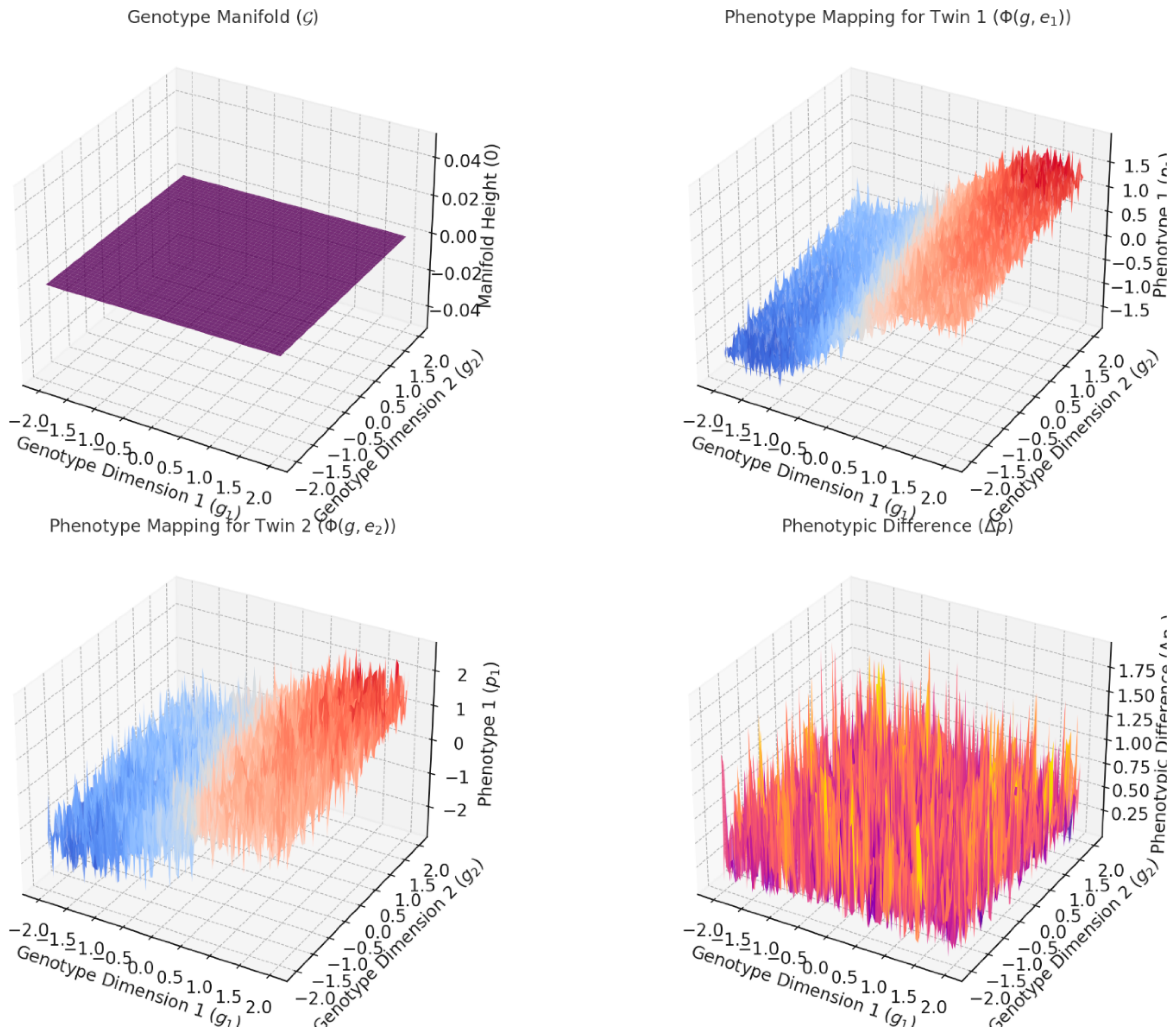
Figure 1 visually demonstrate how differential topology models the relationship between genotypes, phenotypes, and environmental influences, particularly in the context of twin studies. Here's a breakdown of each graph:
This graph is a 2D manifold representing the genetic space, with dimensions and corresponding to genetic variations. The manifold is flat because it represents the initial, untransformed genetic configuration.
This is the starting point for the genotype-to-phenotype mapping. Both twins originate from this shared genetic manifold ( ).
- 2.
Phenotype Mapping for )
This graph shows how Twin 1 's genetic information maps to a phenotype under the influence of environmental factor . The phenotype is a non-linear transformation of the genotype due to environmental perturbations.
The surface illustrates how the environmental factor modifies the genotype manifold into a phenotypic expression. For example, the curvature reflects the genotype-phenotype mapping complexity.
- 3.
Phenotype Mapping for )
This graph is similar to Twin 1's phenotype mapping but reflects a different environmental e2.
This graph is similar to Twin 1's phenotype mapping but reflects a different environmental influence . The resulting phenotype surface differs due to , despite starting from the same genetic manifold.
It highlights the role of environmental variability in shaping phenotypes. The distinct surface compared to Twin 1 shows how even small environmental differences can lead to divergent phenotypes.
- 4.
Phenotypic Difference ( )
This graph quantifies the difference between the phenotypes of the two twins ( . Areas with larger values indicate greater divergence in phenotypic traits due to environmental factors.
This graph encapsulates the key insight from twin studies: while genetics may be shared, environmental influences ( ) drive phenotypic differences. The surface's height highlights regions of significant sensitivity to environmental perturbations.
3.2. Overall Insights
Genetic and Environmental Interaction: The graphs emphasize how the genotype space ( ) interacts with environmental factors to produce phenotypic outcomes .
Environmental Sensitivity: Differences between Twin 1 and Twin demonstrate how even genetically identical individuals can develop distinct traits due to environmental perturbations.
Differential Topology Visualization: The transformations of the flat genotype manifold into curved phenotypic surfaces align with the mathematical framework of differential mappings and perturbations.
These visualizations provide a clear illustration of how twin studies can be modeled mathematically through genotype-phenotype relationships, environmental influences, and their resulting phenotypic differences.
4. Discussion
The divergence of phenotypes in monozygotic (MZ) twins, despite their identical genomic sequences, underscores the complex and dynamic interplay of genetics, environment, and epigenetics. This phenomenon has been widely studied to explore how the same genetic blueprint can give rise to diverse phenotypic traits over time. Factors such as environmental influences, epigenetic modifications, stochastic developmental events, and gene-environment interactions all play roles in generating these differences (Montgomery, 2024)a. This discussion delves into the mechanisms underlying phenotypic divergence in MZ twins, highlighting the interplay between molecular, developmental, and environmental factors.
4.1. Genetic Identity and Early Phenotypic Differences
Monozygotic twins originate from a single zygote that splits during early embryogenesis, resulting in two individuals with identical genetic material. However, even in the earliest stages of development, differences in the twins' intrauterine environment can lead to variability. Placental differences, such as unequal sharing of nutrients or oxygen, can create initial disparities in growth and metabolic programming (Gielen, Lindsey, & Derom, 2008). These subtle differences establish a foundation for future divergence, as environmental and stochastic factors amplify variability over time.
4.2. Epigenetic Modifications as Drivers of Divergence
Epigenetic mechanisms, such as DNA methylation, histone modifications, and non-coding RNAs, regulate gene expression without altering the underlying DNA sequence. These modifications are highly sensitive to environmental stimuli and developmental cues. In twins, differences in epigenetic marks begin to emerge early in life and continue to diverge with age (Fraga et al., 2005). For instance, studies have shown that MZ twins display significant differences in DNA methylation patterns as they grow older, particularly in genes associated with immune response, stress regulation, and metabolism.
Epigenetic drift, the gradual divergence of epigenetic marks over time, is influenced by both stochastic events and environmental exposures. For example, variations in physical activity, diet, and exposure to pollutants can lead to differential methylation of genes, contributing to distinct phenotypes (Feinberg & Irizarry, 2010). In addition, lifestyle differences, such as smoking or alcohol consumption, can accelerate epigenetic changes, amplifying phenotypic divergence (Poulsen et al., 2007).
4.3. Stochastic Developmental Processes
Developmental processes are inherently stochastic, involving random fluctuations in gene expression, protein folding, and cell differentiation. Even in a controlled environment, random events during development can lead to asymmetric cell fates and tissue organization between twins. These stochastic differences are amplified through feedback loops, creating phenotypic disparities that persist throughout life (Raj & van Oudenaarden, 2008).
For instance, during neurodevelopment, stochastic variations in gene expression can influence neural connectivity and synaptic plasticity, resulting in differences in cognitive function and behavior between twins. Such variability highlights the probabilistic nature of development, where small initial differences are magnified over time to produce observable phenotypic traits (McConnell et al., 2017).
4.4. Gene-Environment Interactions
Gene-environment interactions further modulate phenotypic outcomes in twins. While MZ twins share identical genomes, they do not experience identical environments. Differences in physical surroundings, social experiences, and exposure to stressors contribute to divergent phenotypes. For example, one twin exposed to higher levels of early-life stress may develop anxiety or depression, while the other remains unaffected despite sharing genetic susceptibility (Petronis, 2010).
The concept of phenotypic plasticity, or the ability of an organism to modify its phenotype in response to environmental changes, is particularly relevant in twins. Studies have shown that environmental factors can upregulate or downregulate gene expression, leading to changes in traits such as height, weight, and susceptibility to diseases (West-Eberhard, 2003). For instance, one twin may develop obesity due to a sedentary lifestyle, while the other remains lean due to regular physical activity, despite sharing identical genetic predispositions.
4.5. Feedback Mechanisms and Behavioral Reinforcement
Feedback mechanisms between behavior and environment also contribute to phenotypic divergence. Small initial differences in traits or experiences can shape future interactions with the environment, creating a reinforcing cycle. For example, if one twin excels academically, they may receive more encouragement and resources for education, further amplifying cognitive differences. In contrast, the other twin may develop strengths in non-academic areas, leading to divergent life trajectories (Plomin et al., 2013).
This phenomenon is particularly evident in personality and behavioral traits, where twins often exhibit marked differences despite genetic similarity. These differences are shaped by a combination of environmental feedback, personal choices, and social interactions, illustrating the dynamic nature of phenotype formation (Turkheimer & Waldron, 2000).
4.6. Epigenetic Marks and Disease Susceptibility
The divergence of epigenetic marks between twins also explains differences in disease susceptibility. For instance, in twin studies of autoimmune diseases such as rheumatoid arthritis or multiple sclerosis, one twin may develop the condition while the other remains unaffected. These differences are often linked to epigenetic changes in immune-related genes, driven by environmental factors such as infections, diet, or stress (Bell & Saffery, 2012).
Cancer is another area where phenotypic divergence is observed in twins. While MZ twins share genetic predispositions, differences in DNA methylation and histone modifications can influence the activation of oncogenes or the silencing of tumor suppressor genes. Environmental exposures, such as smoking or UV radiation, further exacerbate these differences, leading to variable cancer risk (Fraga et al., 2005).
4.7. Longitudinal Divergence in Twins
Over time, the accumulation of environmental influences and epigenetic changes leads to greater phenotypic divergence in twins. Longitudinal studies have shown that the concordance of traits such as height, weight, and cognitive abilities decreases with age, reflecting the cumulative effects of individual experiences and environmental factors (Boomsma et al., 2002).
For example, studies on the heritability of body mass index (BMI) in twins demonstrate that shared environmental influences are more prominent during childhood, while unique environmental factors become more significant in adulthood. This shift highlights the dynamic nature of gene-environment interactions over the lifespan (Silventoinen et al., 2010).
4.8. Applications of Twin Studies in Research
Twin studies remain a cornerstone of research in genetics, epigenetics, and developmental biology. By comparing phenotypic similarities and differences between MZ and dizygotic (DZ) twins, researchers can estimate the relative contributions of genetic and environmental factors to specific traits. This approach has been instrumental in understanding complex diseases, such as diabetes, schizophrenia, and cardiovascular disorders, where gene-environment interactions play a critical role (Martin et al., 1997).
In addition, advances in sequencing technologies and epigenomic profiling have enabled more detailed analyses of the molecular mechanisms underlying phenotypic divergence in twins. Techniques such as bisulfite sequencing and chromatin immunoprecipitation (ChIP) sequencing have revealed how differential epigenetic modifications contribute to trait variability, providing new insights into the plasticity of the human genome (Jaenisch & Bird, 2003).
4.9. Summary
The divergence of phenotypes in monozygotic twins, despite their shared genetic blueprint, underscores the complexity of the genotype-to-phenotype relationship. Environmental factors, epigenetic modifications, stochastic processes, and feedback mechanisms all contribute to phenotypic variability, highlighting the dynamic and context-dependent nature of development. Twin studies continue to provide a valuable framework for exploring these mechanisms, offering insights into the relative contributions of genetics and environment to human traits and diseases. By integrating advances in genomics, epigenomics, and systems biology, future research will further elucidate the intricate pathways that shape phenotypic diversity over time.
5. Conclusions
The divergence of phenotypes in monozygotic twins, despite their identical genetic material, highlights the intricate interplay between genetic, environmental, epigenetic, and stochastic factors. Environmental exposures, such as nutrition, stress, and social interactions, modify gene expression through epigenetic mechanisms like DNA methylation and histone modification. Over time, these changes, compounded by stochastic developmental processes, lead to significant phenotypic variation.
Twin studies offer a unique framework to disentangle the relative contributions of genetics and environment. Longitudinal analyses reveal how phenotypic concordance decreases with age, reflecting the cumulative impact of individual experiences. Understanding these mechanisms provides insights into human development and the etiology of complex traits and diseases.
Advances in genomic and epigenomic technologies have enabled deeper exploration of the molecular basis of phenotypic divergence, opening avenues for targeted interventions in health and disease. By integrating systems biology with twin studies, future research can further elucidate the genotype-phenotype relationship, contributing to personalized medicine and a deeper understanding of human biology.