Submitted:
26 September 2024
Posted:
26 September 2024
You are already at the latest version
Abstract
In this paper, we conduct a comprehensive analysis of the RounD dataset to enhance the understanding of motion forecasting for autonomous vehicles in complex roundabout environments. We implement a trajectory prediction framework that combines Long Short-Term Memory (LSTM) networks with graph-based modules to model vehicle interactions. Our primary objective is to assess the generalizability of a standard trajectory prediction model across diverse training and testing datasets. Through extensive experiments, we analyze how varying data distributions, including different road configurations and recording times, influence the model’s prediction accuracy and robustness. This study provides key insights into the challenges of domain generalization in autonomous vehicle trajectory prediction.
Keywords:
Machine Learning
; Domain Generalization
; Driving Behavior
; Motion Forecasting
; Trajectory Prediction
1. Introduction
The autonomous vehicle (AV) industry is poised to transform mobility as we know it today, and market projections are expected to be felt worldwide. Motion forecasting is one of the key technologies enabling this transformation, as it gives AVs the ability to predict where other entities like vehicles, pedestrians and road users will be in future [1,2]. As it provides this information to the decision-making algorithms, which in turn help actions like lane changes and collision avoidance, AVs (requires) safe and operational with respect to them [3,4].
But the field struggles a lot. The domain gap between the specialized clips used to train a model and what it perceives as real-world sensory input during driving is one of many major issues. With the motion forecasting landscape for autonomous vehicles being quickly revolutionized, it is becoming increasingly critical to deal with these domain discrepancies. A potentially more fruitful method is transfer learning, which takes data from one area and uses it to improve results in another. This method can be particularly helpful in transitions from urban streets to highways. Transfer learning tends to treat domain misalignment as a source of slowdown, i.e., if the model’s training and application environment are different in terms of accuracy levels, it performs poorly [5]. Domain generalization, on the other hand, is a different scenario: training models across multiple source domains in order to achieve performance that can generalize well when deployed over an unseen environment. It is a necessity for autonomous vehicles that operate in complex, varied environments. However, the major challenge is to generalize in two completely different worlds consistently. Domain adaptation: a proposed technique to combat the source-sample training bias and test-time overfitting through domain transfer, specifically toward bridging data distributions across known sources/domains to new/unfamiliar targets. This is important when the target domain is data-starved. This could be for example a model learned from daytime would not work in nighttime or another weather conditions. The problem lies on how to be easily adapted without a large amount of target domain data [6]. While these approaches show promise, validating effectiveness in the highly dynamic driving environments real-world data is extremely difficult due to variance of scenarios. It reinforces that there is still much work to be done in the years ahead as autonomous vehicles will also need to become some of the safest land pirates on the road [7].
State-of-the-art forecasting methods suffer from requiring datasets that are a simplified version of the messiness in real life [8,9]. Faulty detection/tracking or noisy sensor information from perception layer can also introduce a lot of noise around actual data which with present inside the volumes; leading to motion forecasting models doing even worse [10,11]. A further challenge is that many models under-use available road maps and other contextual information from perception modules, which limits their prediction accuracy in complex or changing environments [12]. Even if we flush out the architectural hypers of different methods in 3D perception active backup, one thing may matter: quality and fidelity of perception input depends on object distances from ego vehicle (a detail oft-ignored across existing forecasting benchmarks) [8].
With these challenges in mind, the demand for end-to-end data analysis has risen when implementing and benchmarking motion forecasting methods. A deep dive into the data can inform these perceptual errors and help us find areas to improve. Therefore, it can promote the development of more solid autoregressive models for understanding and handling increasingly complex real-world driving [8,9]. Moreover, a common evaluation environment must be developed used to benchmark the traditional and end-to-end forecasting approaches against one another [13].
One aspect of understanding the quality and utility of predictions is to understand how different data distributions influence models. Changes like current loci versus rural, day time vs. evening and sundry weather conditions can greatly sway model efficacy[14].For example, a model trained mainly on urban data might not perform well in more rural areas where driving characteristics can diverge. Another one is that, clear-weather models might completely fail to categorize foggy or rainy photos as landscapes [15].
More resilient, generalizable motion forecasting models will need to take into account the effects of data distribution. This helps researchers and practitioners to detect the existence of any bias, and hence adjust the models accordingly such that it can serve well in different life-critical scenarios[8]. For AVs, which are envisaged to operate in a variety of environments and conditions, such an understanding is especially crucial. As such, in order for the field to progress - it is not just beneficial - but absolutely necessary that we carefully examine how different data distributions affect model performance[16].
This paper will use a backbone model including LSTM and graph based method to do the trajectory prediction task. In particular, we perform a distribution analysis of several features by dividing the RounD dataset into several groups that uniformly cover all mentioned traffic scenarios. Contrary to previous works, we contribute a thorough cross-recording comparison within the RounD dataset. With this more nuanced approach, we can target the specific challenges or opportunities related to each traffic condition and thus improve our model’s capacity for accurate predictions of future trajectories. This analysis of driving data and its influence on prediction models provides deep insights for the field of motion prediction in autonomous driving.
2. Related Work
2.1. Trajectory Prediction
Trajectory prediction is fundamental for self-driving vehicles to navigate complex, dynamic scenes safely and efficiently. Deep learning architectures like Generative Adversarial Networks (GANs) and Variational Autoencoders (VAEs) are commonly used for motion forecasting. For example, Social GAN produces socially-aware trajectories by modeling fine-grained interactions among road agents, effectively matching human drivers’ actions [17]. VAEs capture intrinsic motion uncertainty by predicting probability distributions over possible future trajectories, enhancing self-driving capabilities in complex contexts [18]. State-of-the-art approaches like TNT and DenseTNT emphasize temporal features to maintain consistent predictions over time [19,20]. LaneRCNN fuses lane information with road semantics to constrain predictions within reasonable spaces [21]. MultiPath and MultiPath++ predict multiple future trajectory options to handle uncertainties [22,23].
Graph-based networks have become key techniques for trajectory prediction due to their ability to capture complex interactions. GRIP introduced graph structures to model agent interactions [24], leading to rapid developments in the field. Successors like GRIP++ [25] and GISNet [26] further improved graph-based models by considering both spatial and temporal aspects. In our study, we utilize the structure of GRIP++ as our backbone model due to its effectiveness in modeling complex spatiotemporal interactions using graph representations. By modifying the GRU modules and incorporating graph-based feature representations instead of direct coordinate inputs, we aim to use a model that is sufficiently robust and representative.
2.2. Driving Behaviors
Understanding how vehicles operate, especially in the context of autonomous driving, requires a deep dive into driving behavior. Various methods have been used to explore this complex field. For instance, scenario-adaptive techniques help us see how driving behavior changes in different contexts, offering valuable insights into how drivers react to various environments[27]. Researchers also look at the social aspects of driving, examining how vehicles interact with each other and with pedestrians. This helps in understanding the unwritten rules that drivers follow on the road[17]. Following these paper, in order to explore the factors related to driving behaviors, we conduct a comprehensive analysis in multiple ways (e.g., time and agent interactions). By using these diverse methods, we can better understand the intricacies of driving behavior, which is crucial for developing reliable and safe autonomous driving systems. Key factors influencing the analysis of driving behavior include the context in which driving occurs, the inherent unpredictability of human driving habits, and the dynamic interactions between vehicles, pedestrians, and the broader environment. These factors play a pivotal role in shaping the driving behavior observed in real-world scenarios.
2.3. RounD Dataset
RounD was created with the input of researchers working on self-driving technology, and they used that data in addition to a series of challenges (including hierarchical segmentation, keypoint detection for objects other than cars) as benchmarks at CVPR this year. Hundreds of real-world driving scenarios create the data required to learn about vehicle dynamics, interactions and behaviors. On this dataset, the "Scout" study proposed a social-consistency-aware graph attention network for vehicle and Vulnerable Road Users (VRUs) motion forecasting[28]. Other interesting contributions make a specific architecture using deep learning for trajectory prediction and correction, which brings attention to the important point of reliable forecasting needed for safe behavior in vehicle navigation applications[29]. One approach to goal recognition that is not common in this field but allows for fast and interpretable predictions during autonomous driving scenarios multi-av-BJN "GRIT"[30] contrasts above techniques. In this work, we focus on assessing the generalizability of a standard trajectory prediction model across diverse training and testing data from RounD dataset.
2.4. Domain Generalization
In model training tasks, data distribution matters more than we realize - especially in domain generalization. This idea is crucial for making sure that our models are still able to be flexible and generalizable across new environments they have never seen.[31] gave us a nice point of view on domain generalization, making clear that this is one main challenges in order to have models working well in different situations. It is a major pain-point in applications like autonomous driving or industrial automation. To improve on this, [32] propose a fundamentally new way to do trajectory prediction for autonomous vehicles. Their solution is a Graph Neural Network (GNN)-based variant that incorporates domain generalization, the unsolvable problem of universal alignment and adaptation to unseen driving scenarios. This work will adopt GNN-based techniques to deal with the feature representation part in RounD dataset and launch a sophisticated domain generalization analysis between each driving scenario. We believe this work will pave the way for future research on RounD dataset and highllight the importance of domain generalization for reliable autonomous systems.
3. Problem Formulation
We start by defining the trajectory prediction problem: we first formulate the trajectory prediction problem, which involves predicting the future locations of every object in a scene using their past trajectories. To be more specific, our model takes the trajectory histories of all observed objects over time steps as its inputs, denoted as X:
, where
is a coordinates combination of all the observed agents at time and N is the total number of agents. We utilize both world coordinates and relative measurements, such as agent-targeted coordinates. Our objective is to predict the complete trajectories of observed agents over the next steps, which will be represented as the output Y of our model:
Let denote a nonempty input space and the label space. A domain is defined as , where , denotes the label, and represents the joint distribution of the input sample and output label. X and Y denote the corresponding random variables. In domain generalization, we are given M training(source) domains where denotes the domain and denotes a multivariate time series with . We use to represent historical trajectories for a given vehicle A in the domain(map). In this work, the objective is to evaluate the developed predictor f to see if it can maintain its effectiveness across each unseen target domain . (i.e., where , .
4. Overview of the RounD Dataset
For the RoundD dataset, all the recordings are captured under optimal weather conditions, ensuring clear skies, ample lighting, and minimal wind, which enhanced the overall quality of the footage. This guaranteed greater image clarity and stability, simplifying subsequent processing tasks. All footage was recorded using a DJI Phantom 4 Pro drone, which boasts a camera capable of 4K resolution (4096x2160 pixels). The videos are shot at the highest bitrate, capturing 25 frames per second. It successfully extract information on 13,746 road users, i.e., cars (11,530), followed by trucks and vans. Other vehicles like trailers and buses are less common. Vulnerable Road Users (VRUs) such as pedestrians, bicyclists, and motorcyclists are rarer, likely because the roundabouts were situated away from urban centers or shopping districts. The data for each road user includes details like position, heading, speed, and acceleration in both x and y axes of the static UTM coordinate system, as well as in the longitudinal and lateral directions of each participant’s movement.[33]
In Figure 1, we visualize four different types of roundabouts occur from a total of 23 recordings. Among these, Recording has single-lane for all entries and exits and a circular island in the center. Although Recording shares the same shape with Recording, the former is more complex with spiraled traffic lanes to guide vehicles into the correct lane before entering the roundabout and the orientations of the entries and exits are different. The remaining two roundabouts (i.e., Recording 02 and 09) are topologically similar, differing only in their rotations and scales.
5. Dataset Analysis
5.1. Analysis on Recording Types
To analyze the dataset, we first need to understand the data we used on a high-level. For the four selected recordings, the following description demonstrates their corresponding map types (see Figure 1) and the corresponding amount of data in each recording.
Total data means the sum of data amount in each map type. For map type 1, there are no recordings, and the data volume is million, with a total data amount of . In map type 2, there is one recording with a data volume of million, leading to a total data amount of . Map type 3 encompasses recordings numbered 2 through 8, with individual data volumes of , , , , , , and million respectively, accumulating to a total data amount of . Lastly, map type 4 includes recordings numbered 9 to 23, with data volumes ranging from to million. The specific volumes are , , , , , , , , , , , , , , and million respectively, summing up to a total data amount of . This comprehensive data presentation highlights the variations in recording distribution and data volumes across different map types, providing valuable insights for further analysis.
5.2. Analysis on Agent Class Distribution
It is important to recognize the distribution of different agent classes within a given set of input data and why having this knowledge can facilitate the task at hand. What this allows for is a way to figure out who road users are and how they balance or impair traffic with some examples being cars, trucks, people walking. This distribution allows us to at least be aware of possible biases in the data, and attempt overcorrect for it so our models are not overly bias towards one class. This is particularly challenging in motion forecasting fields for autonomous driving as predicting various behaviors of different agents is crucial to ensure the reliability and safety. Improving the robustness and generalizability of our models across diverse real-world scenarios requires that all agent classes are represented in a balanced way.
In Figure 2, we present the distribution of various classes of agents. The Y-axis represents the agent count, while the X-axis enumerates the different agent classes: car, truck, van, trailer, motorcycle, bicycle, bus, and pedestrian. Specifically, we label "car" as the ’Majority’ class (red), and truck, van, trailer as the ’Medium’ class (blue), which are smaller than 10% but higher than 1% of the majority . The ’Minority’ class stands for the remaining four classes, i.e., motorcycle, bicycle, bus and pedestrian, which are less than of the majority. Due to the limited number of observed samples and the significant differences in trajectories between motor vehicles, non-motor vehicles, and pedestrians, we have decided not to include these classes in our analysis. As a result, without loss of generality, we will focus on the interactions and influences between automobiles rather than VRUs to ensure the accuracy of predicted trajectories.
5.3. Analysis on Recording Time Distribution
The time of recording can significantly influence driving behavior due to factors such as traffic density and driver urgency. By analyzing the distribution of recordings across different times of the day, we aim to understand how these temporal variations are represented in our dataset. This knowledge helps us to evaluate whether our models can adapt to different driving conditions encountered at various times. Ensuring that our models perform well under diverse temporal conditions enhances their applicability in real-world scenarios and improves their overall robustness.
In Figure 3, we illustrate the distribution of recordings based on the time of day. The pie chart divides the data into three primary categories: morning, noon, and afternoon. This means that most recordings in the RounD dataset starting in the morning, approximately 30% at noon and only 10% in the afternoon. This type of a distribution offers some hints about the effects that recording times can have on driving behaviors. This figure also shows different trajectory patterns in morning rush hours possibly because drivers would drive more aggressively or think about their works, comparison to for example midday or afternoon as it can be seen from Figure 4. The afternoon, and especially weekends might on the contrary you can take ease when drives or outings by family.[34]. Knowing these day-dependent differences are essential when creating robust prediction models that can adjust to the driving behavior in different times of a single drive [35].
5.4. The Effect of Recording Time to Vehicle State
This section continues exploring how the timestamp alters vehicle states. The idea is to find patterns when they happen at different times of the day, and then predict how these will affect motion forecasting by seeing them. Knowledge of these effects is critical in the modeling of time varying driving behavior.
In Figure 4, we can see that the distribution of velocities and acceleration during morning hours has a wider range compared to that for the afternoon suggesting some driving at constant speed. Perhaps indicative of the need for mobility, drivers tend to accelerate more and can drive argue in regard their velocity. The driving might involve stop-and-go traffic, allowing for quick starts and stops. Velocities and accelerations peak at a lower value than in the morning and afternoon, hinting slower traffic speeds around noon. The driving behavior could be more relaxed with less variability in speed and acceleration, perhaps due to less pressure to reach a destination quickly. The afternoon plot appears to have a wider distribution at higher velocities, possibly indicating faster driving speeds. But the range for acceleration is much less wider than that in the morning, meaning drivers choose to travel in a relatively constant speed rather aggressive driving.
5.5. The Effect of Driving Behaviors to Vehicle State
Understanding the impact of driving behaviors on vehicle states is crucial for developing accurate motion forecasting models. By analyzing how different driving behaviors, such as acceleration, deceleration, and constant speed, influence vehicle states like velocity and acceleration, we can gain valuable insights into the dynamics of driving patterns. This analysis helps us to identify the variations in driving behaviors across different times of the day and under various traffic conditions. By incorporating these behavioral patterns into our models, we can improve their ability to predict vehicle movements more accurately. This step is essential for enhancing the robustness and reliability of our models, ensuring they can effectively handle diverse driving scenarios and provide precise predictions in real-world applications.
According to Figure 5, in the top plot (Velocity), the velocity ranges of road agents are much larger than VRUs and the typical ones are car, truck, van, motorcycle and bus. As similar trend is shown in the bottom plot (Acceleration), we can conclude that velocity has similar impact as acceleration according to the input of motion forecasting.
5.6. Analysis of Feature Correlations
Analyzing the correlations between different features in our dataset provides valuable insights into the relationships among various attributes. This step helps in identifying redundant or highly correlated features, which can be used for feature selection or dimensionality reduction. By understanding these correlations, we can improve the efficiency and performance of our models, ensuring they are trained on the most informative features, thereby enhancing prediction accuracy and simplifying model complexity.
In Figure 6, the correlation matrix shows the correlation between each indicator and checking if there are high connections between them. Warmer colors (like white and light blue) represent higher values, while cooler colors (like dark blues and blue) represent lower values. From that, we can take a deep insight into the relationship between those attributes. I select some important connections that influence the input selection (next part) : both xCenter and yCenter have connections with xVelocity and yVelocity (0.2,0.47 and -0.62,-0.17) and also xVelocity and yVelocity are related to the corresponding Acceleration(0.26 and 0.073). Although most of the absolute values of these data are smaller than 0.5, compared to other figures in this map, they are relatively high values. And the absolute values of all other figures in this map are smaller than 0.1, thus we can assume that there are no strong relationship between each other. Therefore, we can conclude that the pair of center point has linear relationship with velocity and so does velocity with acceleration. From this point, we are able to think of the redundancy of attributes and a way to proceed feature extraction or dimensional reduction.
5.7. Analysis Across Different Scenarios/Maps
To comprehensively evaluate our models, it is essential to test them across different scenarios and maps. This analysis aims to compare the performance of our models in varied environments, identifying any specific challenges or opportunities presented by different traffic conditions. By doing so, we can assess the generalizability and robustness of our models, ensuring they can effectively handle diverse real-world scenarios. This enhances the practicality and reliability of our models in real-world applications.
In this part, we select two different scenarios (Recording 01 and 02) and compare them in various aspects, including class distribution, sample trajectory and average speed, which is important for analyzing the challenges in motion forecasting.
In Figure 7, the majority in all scenarios is car (accounting for more than 75%) and Recording 02 tends to have fewer classes of road agents than the other recordings do. To be more specific, some kinds of vehicles and VRUs are missing in 02, like trailer and bicycles, which account for 0.9%, 1.8% and 0.8%. Recording 01 lacks trucks, and recording 09 lacks pedestrians as well. The percentages of these classes are much lower than others. Therefore, without loss of generosity, we ignore the nuance in both cases in terms of motion forecasting because we pay attention to the movement of agents rather than the catalogs.
The Eq. 1 is used to determine the class of behavior, where stands for the current state of Agent K on Frame i, f represents the evaluate function of driving behavior, which, for this case, is exactly the Acceleration value on both x and y directions. Here we set as a hyperparameter because approximately 80% of agents are lower than as shown in Figure 8. If we use 0 to distinguish between constant speed, acceleration, and deceleration, it becomes challenging to investigate the precise data distribution and to make comparisons with others. This is because maintaining an absolute constant value over a prolonged period is practically unfeasible.
In Figure 8, we can see that in the roundabout scenario, few road agents will remain at a constant velocity during the trip, while the distribution of acceleration and deceleration are shown to be different. The frequency of deceleration is much larger than that of acceleration on all conditions and one significant difference between the four types of recordings is trend of deceleration and acceleration . While those in 01 focus mainly on the ranges [0.2,0.4] and [0.6,0.8], the other three recordings seem to be evenly distributed. But in recording 00, more agents tend to accelerate and there are more acceleartion and deceleration activities in recording 09. According to these difference, we think the main reason is due to different road conditions, such as the number of crossing roads, the number of insections into the main road and the number of agents at that time, which is also an important factor that have a deep impact on motion forecasting.
sectionModel Architecture
5.8. Network Overview
Figure 9 shows the backbone model we used for trajectory prediction. We illustrate the trajectories of all road agents, highlighting the target in orange within the traffic graphs. The orange circle indicates that all agents inside, including the target, are represented as a fixed graph. This graph input is then transformed into several eigenvectors (depicted as green rectangles, with each shade of green representing an eigenvector index) of the original traffic graph. Subsequently, we extract the target eigenvector (orange rectangle) to create a new feature map across all T frames. Using an encoder and decoder, both based on GRU architectures, we predict the final trajectory. Here, D denotes the batch size.
5.9. Graph Representation
We represent each timestamp with n observed road agents using a graph, with the local coordinates of the road agents representing the set of vertices and a set of undirected, weighted edges . All the road agents in this timestamp are considered to be connected with the target agent through bi-directional edges. 1 For agents that have either already left the scene or have not yet appeared, their state is considered unobserved. Consequently, for a given vehicle, its corresponding node feature will either be or the unobserved state .
We chose the GCN structure because it excels at capturing spatial relationships and interactions between entities in a graph, making it ideal for modeling the complex interactions between multiple road agents in autonomous driving scenarios. After we transform all the data into graphs, we then use the GCN [36] to do the feature extraction operation. The layer-wise propagation rule for GCN is given by the following equation:
where represents the activation matrix at the l-th layer, is the activation matrix at the -th layer, is the adjacency matrix of the graph with added self-connections, is the degree matrix of , is the weight matrix for the l-th layer, and denotes the activation function, such as the ReLU function. This rule is applied iteratively to propagate signals through the network.
6. Experiment
6.1. Training Details
We use one Nvidia GeForce RTX 3080 Ti GPU with 16GB memory in the work. We split the whole dataset into four different subsets according to the four map types and for each subset and train it for 50 epochs to generate the best result. To be more specific, we choose 263777, 91971, 150171, 230982 valid trajectories to form the training and testing set, i.e., recording . We train these four recordings in four independent models and test each them on all four senarios to evaluate the in-distribution and out-of-distribution performance of these models. Additionally, we want to compare the model performance at different times, i.e., morning,noon and afternoon. To deal with the data imbalance problem and maintain the same data distribution as the original dataset, we decided to do a stratified sampling on four kinds of recordings (each accounts for ) to obtain two new datasets and compare their performance on each trained models. Besides, we define our problem in 1s observation and 1s prediction, i.e., 25 frames for each.
In terms of the hyperparameters, we use a learning rate of 1e-3, batch size of 256, and choose Adam as the optimizer with weight decay at . Apart from that, the input vectors consist of ten features, i.e., xCenter, yCenter, xVelocity, yVelocity, xAcceleration, yAcceleration, lonVelocity, latVelocity, lonAcceleration, latAcceleration. To extract meaningful features from these high-dimensional data, we need to reduce their dimensionality. In this study, we employ Principal Component Analysis (PCA)[37] to use two attributes instead of the whole ten inputs to represent the majority of road agent features in terms of motion forecasting because we have found the interrelationships between them.Figure 6
Due to the computations involved in obtaining the target agents and their corresponding eigenvectors in GCN feature extraction, we simplify this process by ignoring all the other agents after GCN and only concatenate the dimension of hidden values, where i is the index of target agent.
6.2. Input Format
The input we select are from four independent recordings with the tensor format , with representing for the batch size and standing for 1 second observed data, and 2-dimensional coordinates . The output’s size is the same as the input. When preparing for the dataset, we first select agents according to their types, i.e., excluding the VRUs (bicycle and pedestrian). As discussed before in Section 5.1, the VRUs account for very small percentage of the whole data. And we need to choose an agent i, for the range , we use a slide window to iteratively choose the first 25 frames as training part and the next 25 frames as testing part, where and stand for the first frame and the last frame of agent i.
6.3. Coordinate Transform
Most methods use world spatial coordinates as the input of their models, but there exist some disadvantages to this straightforward way [38]. For example, world coordinates are absolute and can be complex to work with, especially in dynamic environments where many objects are moving simultaneously. Moreover, small errors in world coordinates can lead to significant inaccuracies in trajectory predictions, especially over long distances or durations. In this paper, we use the local coordinate system to transform our dataset. Firstly, we calculate each agent’s coordinates according to the target agent a at timestamp k in the training sequence for both training and predicting, including target agent itself.
where i is in the range of representing different agents, n is the total number of agents. is a certain time step in the existing duration of agent i, and represent the two dimensional coordinates of agent i at moment. In this way, the coordinates of all agents are normalized related to the target agent in the beginning of training.
Subsequently, it has been ascertained that varying scenarios and road conditions exert a considerable influence on the alterations in trajectory prediction, encompassing both longitudinal and lateral dimensions. Consequently, there arises a necessity to establish a novel target-based coordinate system that registers the forward momentum of the target vehicle as the principal axis of variance. By adopting this approach, one can efficaciously transform the global coordinate framework into a localized one.
where is the angle between the agent and the horizontal line (always positive).
The final step is to do the normalization. After the following transformation, we get the trajectory data whose scale is relatively small (the difference of all data in one training sequence is close to the level of 1e-2), which is not beneficial for training the network. So we need to normalize the whole data to the range using MIN-MAX scaler.
where and are the mean and variance of transformed x coordinates in the whole dataset and so are y coordinates.
6.4. Metrics and Loss Function
For this trajectory prediction problem, we use the following standard metrics in our work.
-
ADE(Average Displacement Error): The average euclidean distance between predicted trajectory and the real trajectory., where n indicates the number of vehicles, r indicates the prediction step, indicates the Euclidean distance between the actual and predicted coordinates of vehicle i.
-
FDE(Final Displacement Error): Euclidean distance between trajectory prediction endpoint and true value., where is the end point of the predicted trajectory, and is the end point of the actual trajectory.
In this problem, we use the basic MSE(Mean Squared Error) as the main loss function.
, where n is the total number of data size and are defined as above.
6.5. Results
By observing the table, several general trends and patterns emerge regarding the performance of the models trained and tested on different scenes. Firstly, we notice that the lowest ADE (Average Displacement Error) and FDE (Final Displacement Error) values are generally observed when the training and testing scenes coincide. This indicates that models perform best when applied to the same type of environment they were trained on, highlighting the importance of scene-specific training data. For instance, the model trained and tested on Scene 0 shows relatively low ADE and FDE values ( and , respectively), suggesting high accuracy in predictions for that specific environment. Similarly, we train and test the model on Scene 9 which is made up of simple traffic patterns with high presence of cars giving rise to low error values ( ADE and FDE).
Model trained on complex scenes like Scene 1 have higher error values when tested with other Scenes. The main reason for this is that the sophisticated traffic dynamics and multiple agent types in Scene 1 make it difficult to generalize over other environments. A model trained on Scene 1 would have an ADE of and FDE of when tested in isolation, but with the paired frames from different we can observe that these real values are somewhat close to our predicted ones which further highlights its significance. The prediction for Scene 2, which acquires much more high frequencies of acceleration and deceleration than other scenes, is surprisingly not good, indicated by the higher error values in all models compared to others. However, the model trained on Scene 2 performs significantly better on Scene 9, with an ADE of and an FDE of , indicating some shared characteristics that facilitate better performance.
Overall, the table illustrates that models generally exhibit lower prediction errors when applied to scenes with similar traffic dynamics and agent distributions as their training data. This underscores the importance of accounting for specific scene characteristics during model training to enhance predictive accuracy and generalizability. Additionally, predictable environments with homogeneous agent types, such as Scene 9, tend to yield more accurate predictions across various models, further emphasizing the benefit of training on stable and representative data.
6.5.1. Visualization Analysis
In Figure 10, for recording 0, the predictions by different models are clustered closely around the actual trajectory, as indicated by the yellow dots. The model trained on Recording 0 might be displaying the highest accuracy, given its familiarity with the scene’s dynamics. The model trained on Recording 9 appears to predict the trajectory accurately, which might indicate that the traffic behavior in Recordings 0 and 9 shares similarities that the model can generalize. The divergence between predictions and the ground truth is minimal, suggesting that the models can capture the necessary patterns in such simple scenarios.
For recording 1, the trajectories predicted in this scene show greater divergence, which could be due to the complexity of the scene itself, such as more lanes or higher traffic density. The model trained on Recording 1 likely demonstrates better performance compared to the others, as it would be specialized to the specific complexities of the scene. Models trained on other scenes (models0 2, and 9) might struggle to adapt their predictions to the unique traffic patterns of Recording 1, hence the greater variance in predicted trajectories.
For recording 2, it presents a roundabout with a central island and the complexity of the roundabout interactions is reflected in the more scattered predictions. The model trained on this scene is expected to have learned the nuances of the roundabout’s traffic flow, potentially resulting in closer predictions to the ground truth. Other models seem to have divergent predictions, indicating a lower ability to capture the specific traffic behaviors of this scene, which may be quite different from those in their training data.
For recording 9, the predictions in this scene are relatively close to each other, suggesting that the models find this scene easier to predict or that there is some commonality in the traffic dynamics that all models are able to grasp. Given that the model trained on Recording 9 shows predictions closely following the ground truth, it suggests high accuracy and an understanding of this scene’s particular characteristics. Other models, even though trained on different scenes, seem to provide reasonable predictions for this recording, which may indicate that the traffic patterns in Recording 9 are less unique or that the behaviors here are well-represented in the training datasets of the other models.
7. Conclusions
In this paper, we conducted a thorough analysis of the RounD dataset from various perspectives to enhance the understanding of motion forecasting for autonomous vehicles in roundabout traffic scenarios. Our research focused on evaluating a representative backbone trajectory prediction algorithm, investigating its generalizability across different training and testing datasets. We performed comprehensive experiments to analyze how different data distributions, such as varying road conditions and times of the day, influence the model’s predictive performance. Our study highlighted that models trained on specific types of data tend to perform better when tested on similar data. One key finding is the significant impact of the training and testing dataset composition on the model’s generalizability. Models trained on diverse and representative maps exhibited better generalization to unseen scenarios, underscoring the necessity for comprehensive and varied training data. However, our study has several limitations. The scope of our evaluation is limited to the RounD dataset, which may not fully capture the diversity of real-world driving conditions. Additionally, the current analysis is confined to a single backbone trajectory prediction model. Future work will focus on addressing these limitations by expanding our dataset to include a wider variety of driving conditions. We will also explore generalization analysis across different backbone trajectory prediction models to understand how varying model architectures impact generalization.
Funding
This research received no external funding.
Institutional Review Board Statement
Not applicable.
Informed Consent Statement
Not applicable.
Data Availability Statement
Data are contained within the article.
Conflicts of Interest
The authors declare no conflicts of interest.
References
- Konev, S.; Brodt, K.; Sanakoyeu, A. MotionCNN: A strong baseline for motion prediction in autonomous driving. arXiv preprint 2022, arXiv:2206.02163. [Google Scholar] [CrossRef]
- Mandal, S.; Biswas, S.; Balas, V.E.; Shaw, R.N.; Ghosh, A. Motion prediction for autonomous vehicles from lyft dataset using deep learning. 2020 IEEE 5th International Conference on Computing Communication and Automation (ICCCA). IEEE, 2020, pp. 768–773. [CrossRef]
- Huang, Z.; Mo, X.; Lv, C. ReCoAt: A deep learning-based framework for multi-modal motion prediction in autonomous driving application. 2022 IEEE 25th International Conference on Intelligent Transportation Systems (ITSC). IEEE, 2022, pp. 988–993. [CrossRef]
- Khandelwal, S.; Qi, W.; Singh, J.; Hartnett, A.; Ramanan, D. What-if motion prediction for autonomous driving. arXiv preprint 2020, arXiv:2008.10587. [Google Scholar] [CrossRef]
- Kothari, P.; Li, D.; Liu, Y.; Alahi, A. Motion style transfer: Modular low-rank adaptation for deep motion forecasting. Conference on Robot Learning. PMLR, 2023, pp. 774–784.
- Hu, Y.; Jia, X.; Tomizuka, M.; Zhan, W. Causal-based time series domain generalization for vehicle intention prediction. 2022 International Conference on Robotics and Automation (ICRA). IEEE, 2022, pp. 7806–7813. [CrossRef]
- Chen, W.; Yu, Z.; Wang, Z.; Anandkumar, A. Automated synthetic-to-real generalization. International Conference on Machine Learning. PMLR, 2020, pp. 1746–1756.
- Xu, Y.; Chambon, L.; Zablocki, É.; Chen, M.; Cord, M.; Pérez, P. Challenges of Using Real-World Sensory Inputs for Motion Forecasting in Autonomous Driving. arXiv preprint 2023, arXiv:2306.09281. [Google Scholar] [CrossRef]
- Aoki, S.; Lin, C.W.; Rajkumar, R. Human-robot cooperation for autonomous vehicles and human drivers: Challenges and solutions. IEEE communications magazine 2021, 59, 35–41. [Google Scholar] [CrossRef]
- Gulzar, M.; Muhammad, Y.; Muhammad, N. A survey on motion prediction of pedestrians and vehicles for autonomous driving. IEEE Access 2021, 9, 137957–137969. [Google Scholar] [CrossRef]
- Ghorai, P.; Eskandarian, A.; Kim, Y.K.; Mehr, G. State estimation and motion prediction of vehicles and vulnerable road users for cooperative autonomous driving: A survey. IEEE transactions on intelligent transportation systems 2022, 23, 16983–17002. [Google Scholar] [CrossRef]
- Benrachou, D.E.; Glaser, S.; Elhenawy, M.; Rakotonirainy, A. Use of social interaction and intention to improve motion prediction within automated vehicle framework: A review. IEEE Transactions on Intelligent Transportation Systems 2022. [Google Scholar] [CrossRef]
- Karle, P.; Geisslinger, M.; Betz, J.; Lienkamp, M. Scenario understanding and motion prediction for autonomous vehicles—review and comparison. IEEE Transactions on Intelligent Transportation Systems 2022, 23, 16962–16982. [Google Scholar] [CrossRef]
- Djuric, N.; Radosavljevic, V.; Cui, H.; Nguyen, T.; Chou, F.C.; Lin, T.H.; Singh, N.; Schneider, J. Uncertainty-aware short-term motion prediction of traffic actors for autonomous driving. Proceedings of the IEEE/CVF Winter Conference on Applications of Computer Vision, 2020, pp. 2095–2104. [CrossRef]
- Shao, W.; Xu, Y.; Li, J.; Lv, C.; Wang, W.; Wang, H. How Does Traffic Environment Quantitatively Affect the Autonomous Driving Prediction? IEEE Transactions on Intelligent Transportation Systems 2023. [Google Scholar] [CrossRef]
- Ren, X.; Yang, T.; Li, L.E.; Alahi, A.; Chen, Q. Safety-aware motion prediction with unseen vehicles for autonomous driving. Proceedings of the IEEE/CVF International Conference on Computer Vision, 2021, pp. 15731–15740. [CrossRef]
- Gupta, A.; Johnson, J.; Fei-Fei, L.; Savarese, S.; Alahi, A. Social gan: Socially acceptable trajectories with generative adversarial networks. Proceedings of the IEEE conference on computer vision and pattern recognition, 2018, pp. 2255–2264. [CrossRef]
- De Miguel, M.Á.; Armingol, J.M.; García, F. Vehicles trajectory prediction using recurrent VAE network. IEEE Access 2022, 10, 32742–32749. [Google Scholar] [CrossRef]
- Zhao, H.; Gao, J.; Lan, T.; Sun, C.; Sapp, B.; Varadarajan, B.; Shen, Y.; Shen, Y.; Chai, Y.; Schmid, C. ; others. Tnt: Target-driven trajectory prediction. Conference on Robot Learning. PMLR, 2021, pp. 895–904. [CrossRef]
- Gu, J.; Sun, C.; Zhao, H. Densetnt: End-to-end trajectory prediction from dense goal sets. Proceedings of the IEEE/CVF International Conference on Computer Vision, 2021, pp. 15303–15312. [CrossRef]
- Zeng, W.; Liang, M.; Liao, R.; Urtasun, R. Lanercnn: Distributed representations for graph-centric motion forecasting. 2021 IEEE/RSJ International Conference on Intelligent Robots and Systems (IROS). IEEE, 2021, pp. 532–539. [CrossRef]
- Chai, Y.; Sapp, B.; Bansal, M.; Anguelov, D. Multipath: Multiple probabilistic anchor trajectory hypotheses for behavior prediction. arXiv preprint 2019, arXiv:1910.05449. [Google Scholar] [CrossRef]
- Varadarajan, B.; Hefny, A.; Srivastava, A.; Refaat, K.S.; Nayakanti, N.; Cornman, A.; Chen, K.; Douillard, B.; Lam, C.P.; Anguelov, D. ; others. Multipath++: Efficient information fusion and trajectory aggregation for behavior prediction. 2022 International Conference on Robotics and Automation (ICRA). IEEE, 2022, pp. 7814–7821. [CrossRef]
- Li, X.; Ying, X.; Chuah, M.C. Grip: Graph-based interaction-aware trajectory prediction. 2019 IEEE Intelligent Transportation Systems Conference (ITSC). IEEE, 2019, pp. 3960–3966. [CrossRef]
- Li, X.; Ying, X.; Chuah, M.C. Grip++: Enhanced graph-based interaction-aware trajectory prediction for autonomous driving. arXiv preprint 2019, arXiv:1907.07792. [Google Scholar] [CrossRef]
- Zhao, Z.; Fang, H.; Jin, Z.; Qiu, Q. Gisnet: Graph-based information sharing network for vehicle trajectory prediction. 2020 International Joint Conference on Neural Networks (IJCNN). IEEE, 2020, pp. 1–7. [CrossRef]
- Geng, X.; Liang, H.; Yu, B.; Zhao, P.; He, L.; Huang, R. A scenario-adaptive driving behavior prediction approach to urban autonomous driving. Applied Sciences 2017, 7, 426. [Google Scholar] [CrossRef]
- Carrasco, S.; Llorca, D.F.; Sotelo, M. Scout: Socially-consistent and understandable graph attention network for trajectory prediction of vehicles and vrus. 2021 IEEE Intelligent Vehicles Symposium (IV). IEEE, 2021, pp. 1501–1508. [CrossRef]
- Hui, F.; Wei, C.; ShangGuan, W.; Ando, R.; Fang, S. Deep encoder–decoder-NN: A deep learning-based autonomous vehicle trajectory prediction and correction model. Physica A: Statistical Mechanics and its Applications 2022, 593, 126869. [Google Scholar] [CrossRef]
- Brewitt, C.; Gyevnar, B.; Garcin, S.; Albrecht, S.V. GRIT: Fast, interpretable, and verifiable goal recognition with learned decision trees for autonomous driving. 2021 IEEE/RSJ International Conference on Intelligent Robots and Systems (IROS). IEEE, 2021, pp. 1023–1030. [CrossRef]
- Patricia, N.; Caputo, B. Learning to learn, from transfer learning to domain adaptation: A unifying perspective. Proceedings of the IEEE conference on computer vision and pattern recognition, 2014, pp. 1442–1449. [CrossRef]
- Xu, Y.; Wang, L.; Wang, Y.; Fu, Y. Adaptive trajectory prediction via transferable gnn. Proceedings of the IEEE/CVF Conference on Computer Vision and Pattern Recognition, 2022, pp. 6520–6531. [CrossRef]
- Krajewski, R.; Moers, T.; Bock, J.; Vater, L.; Eckstein, L. The round dataset: A drone dataset of road user trajectories at roundabouts in germany. 2020 IEEE 23rd International Conference on Intelligent Transportation Systems (ITSC). IEEE, 2020, pp. 1–6. [CrossRef]
- Sarkar, A.; Czarnecki, K.; Angus, M.; Li, C.; Waslander, S. Trajectory prediction of traffic agents at urban intersections through learned interactions. 2017 IEEE 20th International Conference on Intelligent Transportation Systems (ITSC). IEEE, 2017, pp. 1–8. [CrossRef]
- Lyu, N.; Wen, J.; Duan, Z.; Wu, C. Vehicle trajectory prediction and cut-in collision warning model in a connected vehicle environment. IEEE Transactions on Intelligent Transportation Systems 2020, 23, 966–981. [Google Scholar] [CrossRef]
- Zhang, S.; Tong, H.; Xu, J.; Maciejewski, R. Graph convolutional networks: A comprehensive review. Computational Social Networks 2019, 6, 1–23. [Google Scholar] [CrossRef] [PubMed]
- Kurita, T. Principal component analysis (PCA). Computer Vision: A Reference Guide 2019, pp. 1–4. [CrossRef]
- Vilardaga García-Cascón, S. An integrated framework for trajectory optimisation, prediction and parameter estimation for advanced aircraft separation concepts 2019. [CrossRef]
| 1 | For target agent a and for each other agent node i, we will get and . |
Figure 1.
All four kinds of recordings in RounD dataset
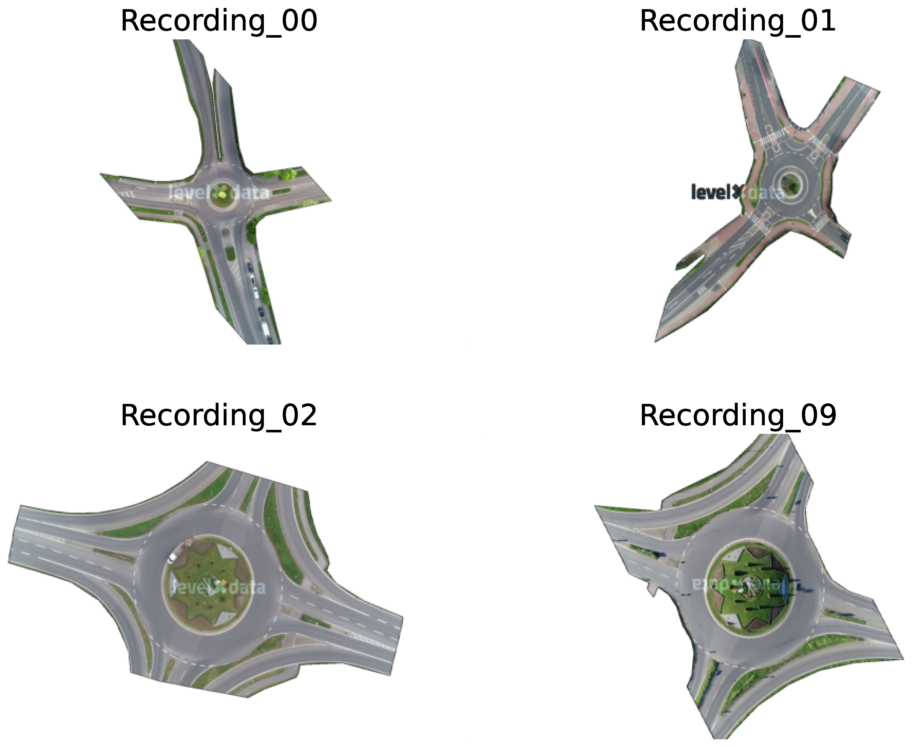
Figure 2.
Class distribution among all recordings
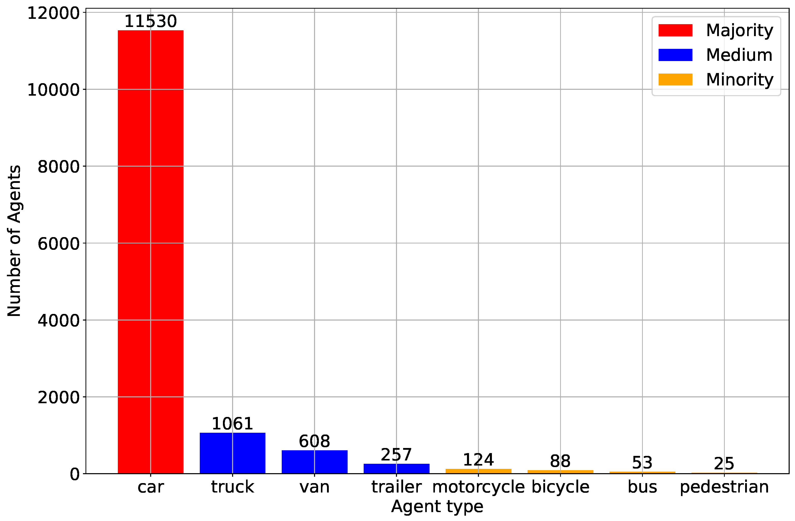
Figure 3.
Distribution Of Time Distribution
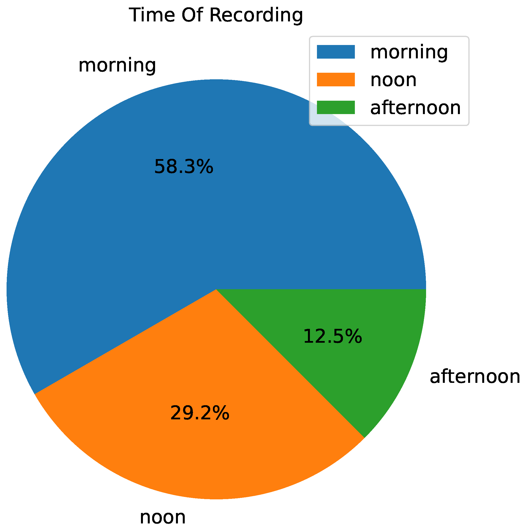
Figure 4.
Distribution of vehicles’ velocity and acceleration for morning and afternoon recordings.

Figure 5.
Distribution of Velocity and Acceleration according to different road agent groups on the whole dataset.
Figure 5.
Distribution of Velocity and Acceleration according to different road agent groups on the whole dataset.
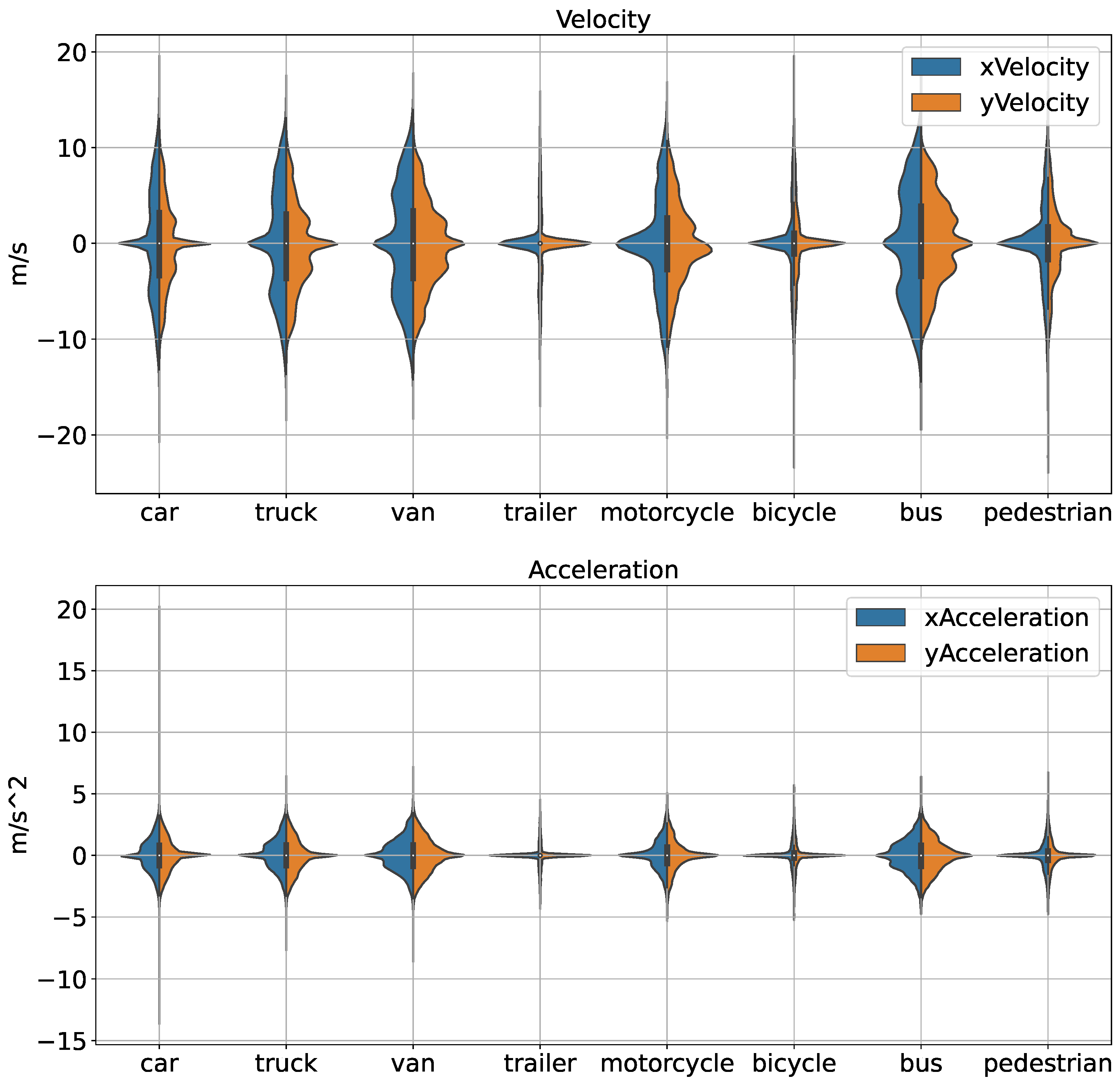
Figure 6.
Heatmap for all attributes on RounD dataset.
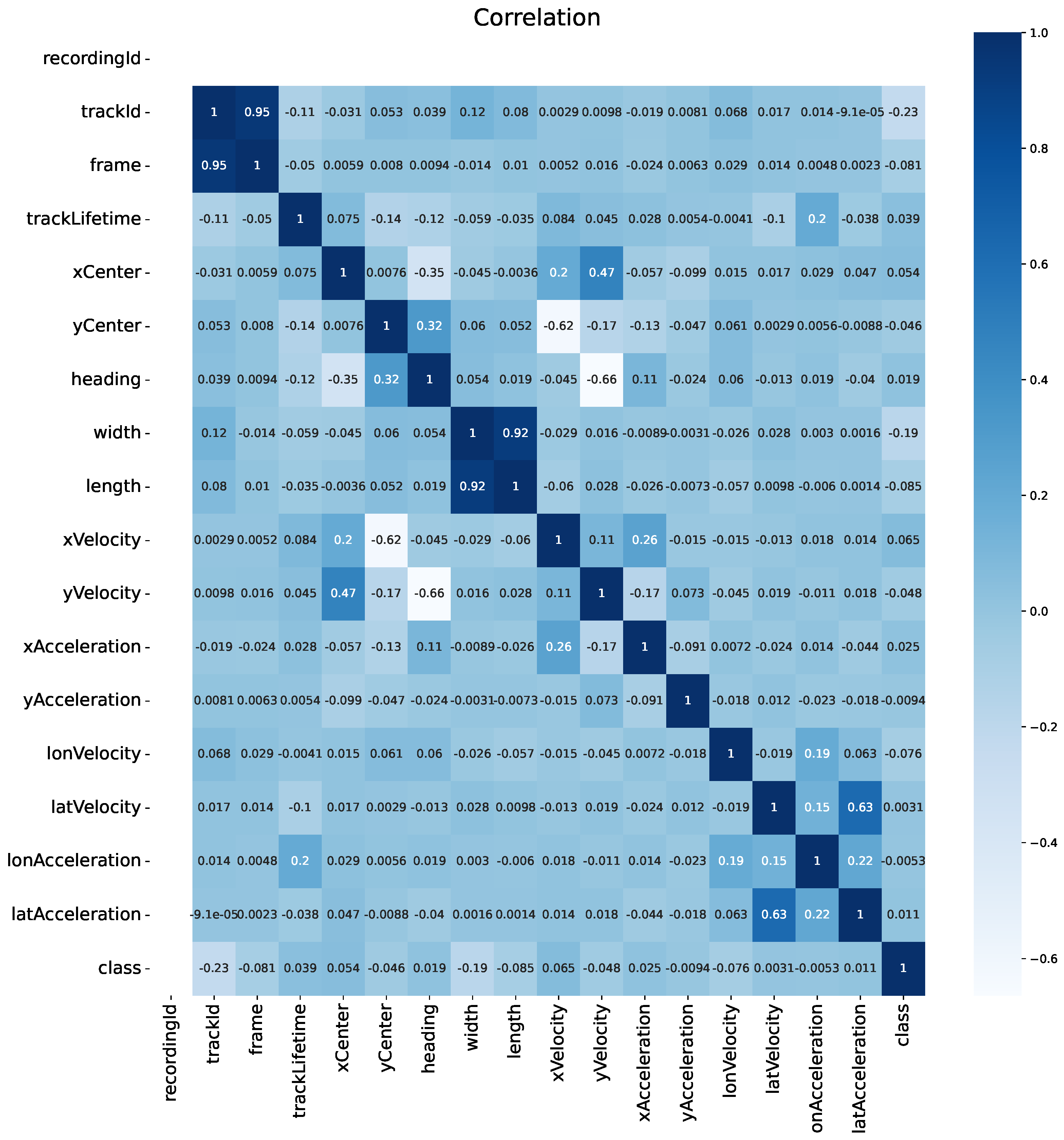
Figure 7.
Comparison of class distribution.
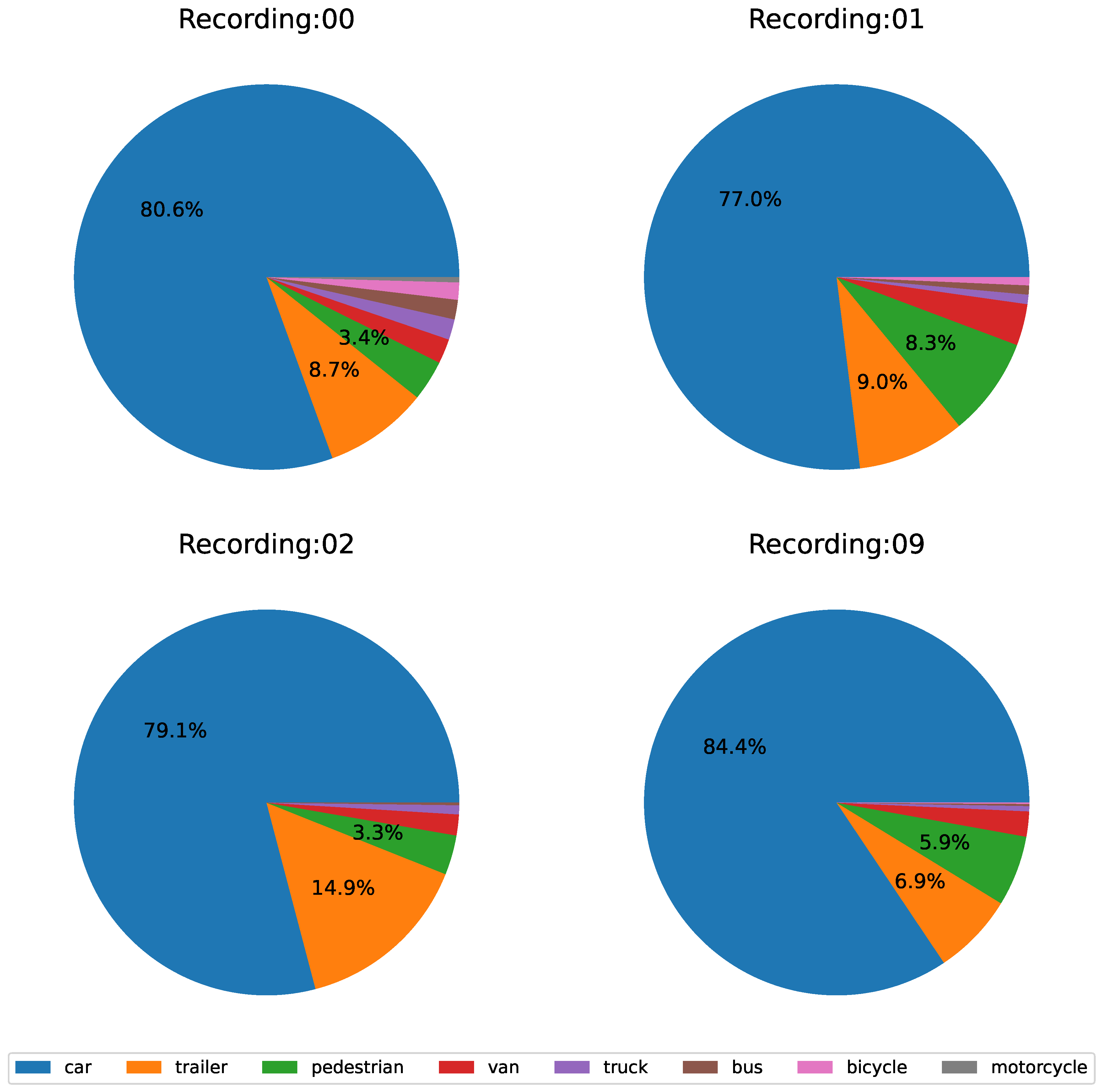
Figure 8.
Distribution of acceleration-deceleration behaviors for road agents in two separate recordings.
Figure 8.
Distribution of acceleration-deceleration behaviors for road agents in two separate recordings.
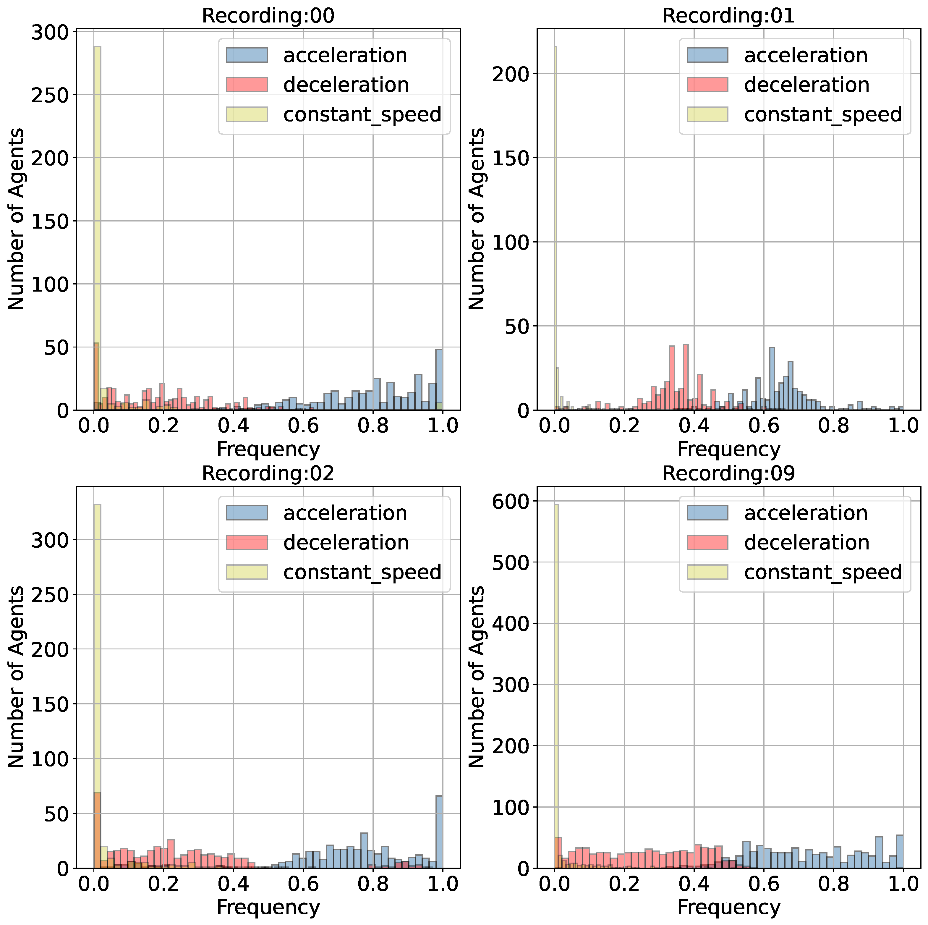
Figure 9.
Overall architecture of the backbone trajectory prediction model used in our paper.
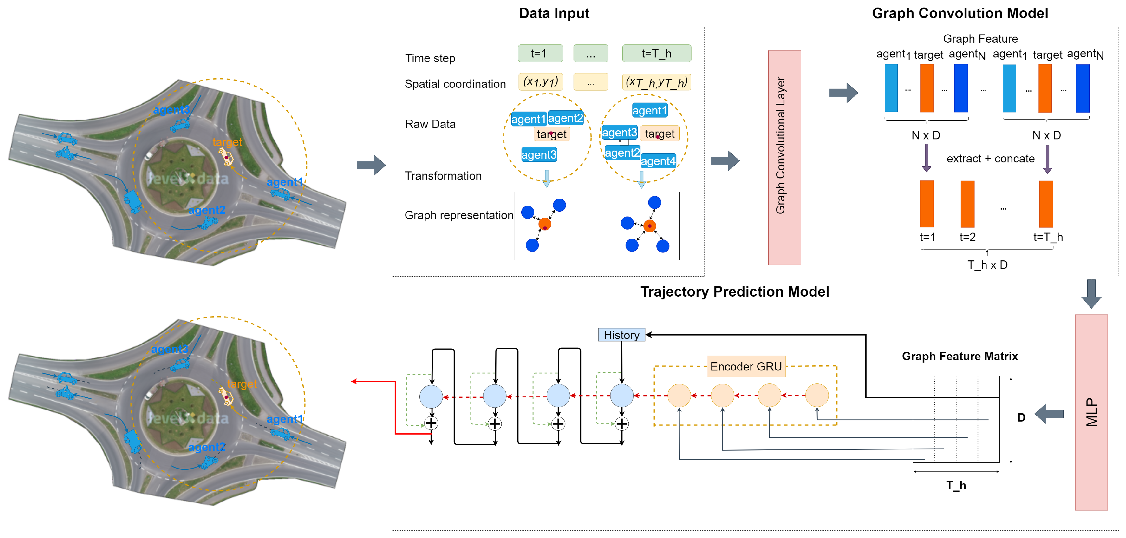
Figure 10.
Visualized Prediction Results. Target vehicle is colored in orange and all other agents are colored in blue. Blue and yellow points are the trajectory history and labels of all the road-agents. Black triangles are the predicted trajectories of the target agent in model 0. Red crosses represents model 1, green pluses and pink points are model 2 and model 9 seperately.


Table 1.
This table shows the ADE and FDE metrics calculated from all the types of recordings in all the trained models.
Table 1.
This table shows the ADE and FDE metrics calculated from all the types of recordings in all the trained models.
| training | |||||
| ADE \FDE | 0 | 1 | 2 | 9 | |
| testing | 0 | 0.81 \1.06 | 1.08 \1.24 | 1.34 \1.69 | 1.12 \1.42 |
| 1 | 0.88 \1.14 | 0.87 \1.34 | 1.23 \1.43 | 0.93 \1.43 | |
| 2 | 0.99 \1.05 | 1.29 \1.96 | 0.28 \0.49 | 0.57 \0.62 | |
| 9 | 1.09 \1.34 | 1.46 \1.78 | 0.79 \0.82 | 0.16 \0.31 | |
Disclaimer/Publisher’s Note: The statements, opinions and data contained in all publications are solely those of the individual author(s) and contributor(s) and not of MDPI and/or the editor(s). MDPI and/or the editor(s) disclaim responsibility for any injury to people or property resulting from any ideas, methods, instructions or products referred to in the content. |
© 2024 by the authors. Licensee MDPI, Basel, Switzerland. This article is an open access article distributed under the terms and conditions of the Creative Commons Attribution (CC BY) license (http://creativecommons.org/licenses/by/4.0/).
Copyright: This open access article is published under a Creative Commons CC BY 4.0 license, which permit the free download, distribution, and reuse, provided that the author and preprint are cited in any reuse.


