Instrument Selection in Panel Data Models with Endogeneity: A Bayesian Approach

Preprint

Article

Instrument Selection in Panel Data Models with Endogeneity: A Bayesian Approach

This version is not peer-reviewed.

Álvaro Herce Postigo^*

Manuel Salvador

Álvaro Herce Postigo^*

Manuel Salvador

This version is not peer-reviewed.

Altmetrics

Downloads

Views

Comments

Submitted:

31 October 2024

Posted:

01 November 2024

You are already at the latest version

A peer-reviewed article of this preprint also exists.

Abstract

This paper proposes the use of Bayesian inference techniques to search for and obtain valid instruments in dynamic panel data models where endogenous variables may exist. The use of Principal Component Analysis (PCA) allows for obtaining a reduced number of instruments in comparison to the high number of instruments commonly used in the literature, and Monte Carlo Markov Chain (MCMC) methods enable efficient exploration of the instrument space, deriving accurate point estimates of the elements of interest. The proposed methodology is illustrated in a simulated case and in an empirical application, where the partial effect of a series of determinants on the attraction of international bank flows is quantified. The results highlight the importance of promoting and developing the private sector in these economies, as well as the importance of maintaining good levels of credit worthiness.

Keywords:

Subject:

Business, Economics and Management - Econometrics and Statistics

1. Introduction

Endogeneity is a common issue in economic research that can lead to biased and inconsistent estimates if not properly addressed. Instrumental variables are typically employed to mitigate this problem. These variables must satisfy two key conditions: they must be uncorrelated with the error term of the regression model (exogeneity condition) and correlated with the endogenous variables (relevance condition). By using these instruments as regressors instead of the endogenous variables, it is possible to obtain asymptotically unbiased estimates of the regression coefficients.

In panel data modelling, estimation techniques based on the Generalized Method of Moments (GMM) are commonly used (Arellano & Bond, 1991; Arellano & Bover, 1995). To apply GMM, a system of equations is specified. The first equation captures the relationship between the dependent variable and a set of explanatory variables, which may include both strictly exogenous and endogenous variables. The remaining equations describe the interdependencies between the endogenous variables and a set of regressors or instrumental variables. These instruments are intended to maximize the information about the endogenous variables (relevance condition) while ensuring they do not introduce bias into the estimation of the first equation due to their orthogonality with the error term (exogeneity condition).

Under certain regularity conditions, the GMM estimation procedure is asymptotically unbiased and efficient (Roodman, 2009b). However, this method faces several limitations. One significant challenge is the high dimensionality of the instrument set. As GMM methodology constructs instruments based on orthogonality conditions between the idiosyncratic error and the instruments, the number of instruments increases quadratically with the length of the time series, leading to a trade-off between efficiency gains from incorporating additional moments and the loss of degrees of freedom. Moreover, while the orthogonality conditions generally ensure the exogeneity of instruments, they do not guarantee the relevance condition, which is a critical issue addressed in this study.

To reduce the number of instruments, Roodman (2009 a, b) proposed collapsing the instrument matrix. While effective in many cases, this approach can still result in high-dimensional matrices, particularly in contexts with a large number of time observations, and it does not differentiate between relevant and irrelevant instruments. Nevertheless, the approach of constructing instrumental matrices using lags of the endogenous variables, combined with dimensional reduction through matrix collapsing, provides a useful starting point for applying GMM in panel models, including non-dynamic ones, where suitable instruments may be scarce.

Building upon the methodology introduced in this paper, we propose leveraging Principal Component Analysis (PCA) in conjunction with Bayesian methods to select a reduced set of valid instruments, thereby enhancing estimation efficiency without compromising precision in the parameters of interest. Initially, we apply PCA to the instrument matrix to mitigate multicollinearity among the instruments and to extract the most informative components. Next, we model each endogenous variable as a function of these transformed, orthogonal instruments. The estimation of these relationships is conducted using Gibbs Sampling with non-informative priors on the parameters, allowing for flexible and robust inference. This Bayesian approach enables us to identify the most relevant instruments that are significant at a minimum credibility level of 90%. By incorporating Bayesian techniques, we achieve a parsimonious instrument set that maintains the model’s goodness of fit, effectively balancing complexity and estimation accuracy. For a more comprehensive exposition on the application of Bayesian methods in panel data contexts, interested readers are referred to (Chib, 2008).

The proposed methodology is illustrated by applying it to simulated cases and to an empirical study focuses on understanding the influence of economic, financial, and governance indicators on international bank inflows in emerging economies, drawing on the work of (Kim & Wu, 2008). By examining 50 countries over a 26-year period, this study highlights the role of the public sector in fostering capital inflows and evaluates which indicators act as significant pull factors for bank capital, versus those that might deter such inflows. It addresses the methodological challenges of endogeneity within governance indicators by implementing a forward orthogonal deviation transformation and utilizing a fixed effects instrumental variable approach. The results reveal that economic and financial variables, such as GDP per capita and credit ratings, are prominent attractors, while governance indicators like government effectiveness can present a latent effect undiscovered by endogeneity on data, shaping the policy implications for emerging markets.

The remainder of the paper is organized as follows. Section 2 introduces the problem, assuming the presence of an endogenous regressor. Section 3 outlines the process of identifying valid instruments that satisfy the relevance and exogeneity conditions while minimizing their number. Section 4 details the posterior inference procedure for the model parameters following the identification of the necessary instruments. In Section 5, we evaluate the performance of the proposed methodology using a simulated example. Section 6 presents the empirical study, where we analyse the partial effects of governance indicators on bank capital inflows. Section 7 concludes the paper. Supplementary material includes three appendices: Appendix A provides a detailed mathematical derivation of key results, Appendix B offers a description of the variables, and Appendix C presents additional supporting information.

2. Setting-Up the problem

Let

\{y_{i t}, \{x_{j i t}, j = 1,2, . . . ., K_{x}\}, \{w_{j i t}, j = 1,2, . . ., K_{w}\}; i = 1, . . ., N; t = 1, . . ., T\}

be a balanced panel dataset corresponding to N individual units and T periods, where y is the dependent variable,

X = (X_{1}, \dots, X_{K_{x}})

are explanatory strictly exogenous variables and

W = (W_{1}, \dots, W_{K_{w}})

are endogenous explanatory variables. Without loss of generality, we assume that

K_{w} = 1

, with an extension to the case of

K_{w} > 1

being straightforward (see Section 4.4 below).

Let us assume a dynamic panel model with individual effects given by:

y_{i t} = β_{0} y_{i, t - 1} + \underset{j = 1}{\sum^{K_{x}}} x_{j i t} β_{1 j} + w_{i t} β_{2} + α_{i} + u_{i t}

(2.1)

which describes the evolution of the variable of interest

y

, where

\{α_{i}, i = 1,2, . . ., N\}

are individual fixed effects and

\{u_{i t}; i = 1, \dots, N; t = 1, \dots, T\}

are i.i.d. homoscedastic random normal disturbances, with

u_{i t} \sim N (0, σ_{u}^{2})

. The main concern is the estimation of

β_{2}

, the direct effect of W on y.

To eliminate bias in the estimation of

β_{2}

, we consider a set of KZ instrumental variables

Z = (Z_{1}, \dots, Z_{K_{z}})

with observed values

\{z_{j i t}, j = 1,2, . . ., K_{z}; t = 1, \dots, T; i = 1, \dots, N\}

, which are assumed to be related to the variable

W

(relevance condition) by means of the linear regression:

w_{i t} = \underset{j = 1}{\sum^{K_{Z}}} z_{j i t} ϕ_{j} + ϵ_{i t}

(2.2)

with

\{ϵ_{i t} \sim N (0, σ_{ϵ}^{2}); t = 1, \dots, T; i = 1, \dots, N\}

. The instrumental variables Z are supposed to be uncorrelated with the random disturbances

\{u_{i t}; t = 1, \dots, T; i = 1, \dots, N\}

in such a way that

cov (z_{j i t}, u_{i t}) = 0, \forall i, t

(exogeneity condition), and it is possible to consider including those variables that are marked as strictly exogenous in the model. In the best-case scenario, the use of instrumental variables that meet the aforementioned conditions and are available to the researcher is considered. However, in reality, these variables are often unknown and not externally accessible, making it necessary to use the available sample information to generate them. In addition, it is assumed that:

\begin{matrix} cov (u_{i t}, x_{j i t}) = cov (ε_{i t}, z_{j i t}) = cov (ε_{i t}, x_{j i t}) = 0 \forall i, j, t \\ cov ((u_{i t}, ε_{i t}), (u_{j t}, ε_{j t})) = 0 \forall i \neq j \\ (u_{i t}, ε_{i t}) \sim N ([\begin{matrix} 0 \\ 0 \end{matrix}], [\begin{matrix} σ_{u}^{2} & σ_{u, ε} \\ σ_{u, ε} & σ_{ε}^{2} \end{matrix}]) \end{matrix}

(2.3)

where

σ_{u, ε} = cov (u_{i t}, ε_{i t})

. The endogeneity problem arises when

σ_{u, ε} = cov (u_{i t}, ε_{i t}) \neq 0

, which lead to bias in the inference about the parameter

β_{2}

, which does not disappear asymptotically. This bias can be overcome using instrumental variables that verify the conditions of relevance

(\exists j \in \{1, . . ., K_{z}\} : ϕ_{j} \neq 0)

, and exogeneity

(cov (z_{j i t}, u_{i t}) = 0); \forall j

. However, it is usual to choose the instrumental variables Z using doubtful ad hoc subjective value judgements. Commonly used procedures, even those proposed by (Roodman, 2009 a, b), can generate a large number of instruments, increasing the computational complexity of the procedure, as well as the existence of multicollinearity problems between the instruments, reducing the precision of the inferences.

In this paper, we propose a Bayesian methodology to estimate

β_{2}

providing, on one hand, a general methodology to obtain valid instruments generated from sample information, using relevant moment conditions and, on the other hand, a procedure to reduce the size of the generated matrix of instruments by mitigating the likelihood of quasi-multicollinearity among instruments.

3. Methodology

3.1. General Setting and Forward Orthogonal Deviations

We present a general methodology for dealing with endogenous variables using only one endogenous regressor. Application to more than one endogenous regressor is straightforward, and general guidelines are provided below (see Section 4.4). The starting point is the equation system defined by:

\begin{matrix} y_{i t} = β_{0} y_{i, t - 1} + \sum_{j = 1}^{K_{x}} x_{j i t} β_{1 j} + w_{i t} β_{2} + α_{i} + u_{i t} \\ w_{i t} = \sum_{j = 1}^{K_{z}} z_{j i t} ϕ_{j} + ε_{i t} \end{matrix}

(3.1)

In panel data settings, a source of potential endogeneity is the value of

cov (y_{i, t - 1}, α_{i})

, but one can apply some of the common transformations to eliminate individual effects while retaining sample information. Our proposal is to employ a forward orthogonal deviations (FOD) transformation (Arellano & Bover, 1995). For each element included in the model, the transformation is given by:

\begin{matrix} {\tilde{y}}_{i t} = {[\frac{T - t}{T - t + 1}]}^{\frac{1}{2}} [y_{i t} - \frac{1}{T - t} \underset{s = t + 1}{\overset{T}{\sum y_{i s}}}] \\ {\tilde{x}}_{j i t} = {[\frac{T - t}{T - t + 1}]}^{\frac{1}{2}} [x_{j i t} - \frac{1}{T - t} \underset{s = t + 1}{\overset{T}{\sum x_{j i s}}}] \\ \begin{matrix} {\tilde{z}}_{j i t} = {[\frac{T - t}{T - t + 1}]}^{\frac{1}{2}} [z_{j i t} - \frac{1}{T - t} \underset{s = t + 1}{\overset{T}{\sum z_{j i s}}}] \\ {\tilde{w}}_{i t} = {[\frac{T - t}{T - t + 1}]}^{\frac{1}{2}} [w_{i t} - \frac{1}{T - t} \underset{s = t + 1}{\overset{T}{\sum w_{i s}}}] \\ \begin{matrix} {\tilde{u}}_{i t} = {[\frac{T - t}{T - t + 1}]}^{\frac{1}{2}} [u_{i t} - \frac{1}{T - t} \underset{s = t + 1}{\overset{T}{\sum u_{i s}}}] \\ {\tilde{ε}}_{i t} = {[\frac{T - t}{T - t + 1}]}^{\frac{1}{2}} [ε_{i t} - \frac{1}{T - t} \underset{s = t + 1}{\overset{T}{\sum ε_{i s}}}] \end{matrix} \end{matrix} \end{matrix}

(3.2)

which, applied to the system (3.1) resulting in:

\begin{matrix} {\tilde{y}}_{i t} = β_{0} {\tilde{y}}_{i, t - 1} + \underset{j = 1}{\sum^{K_{x}}} {\tilde{x}}_{j i t} β_{1 j} + {\tilde{w}}_{i t} β_{2} + {\tilde{u}}_{i t} \\ {\tilde{w}}_{i t} = \underset{j = 1}{\sum^{K_{z}}} {\tilde{z}}_{j i t} ϕ_{j} + {\tilde{ε}}_{i t} \end{matrix}

(3.3)

Thus, the fixed effects

α_{i}

are removed from (3.1). When dealing with an unbalanced panel, as pointed out by (Roodman, 2009b), the Forward Orthogonal Deviation Transformation fills the gaps with the average of all future available observations of a variable, minimizing data loss. Practically, this is equivalent to replace the missing value as a zero value.

This approach offers the advantage that, provided the original errors are homoscedastic and uncorrelated, these properties are preserved unchanged after transformation. Prior plausible alternative transformations include the Within transformation and the first-difference (FD) transformation. However, the Within transformation must be excluded in a dynamic context because it incorporates time-specific realizations, leading to correlation with each lag of the variable. With respect to the first-difference transformation, although is straightforward to implement, it presents significant drawbacks compared to the orthogonal deviations transformation. Specifically, the first observation for each individual in the sample must be omitted, it induces autocorrelation between consecutive errors, and the first lag of the endogenous variable is lost as an instrumental variable. For a more comprehensive discussion see (Croissant & Millo, 2019; Mátyás & Sevestre, 2008).

3.2. Over-Dimensionality Problems

From a frequentist perspective, the Generalized Method of Moments (GMM) approach has usually been considered for the inference process because of its flexibility and because it requires adopting very few assumptions about the data-generating process. In addition, most proposed versions provide estimates that prevent the well-known (Nickell, 1981) bias from appearing. However, this method has some shortcomings. The main one is the way the instrumental variables are introduced. Using the approach of (Holtz-Eakin et al., 1988), the number of valid instruments is

N T \times \frac{T (T - 1)}{2}

, which can cause problems in the finite samples. One of problems is the dimension of the resultant variance matrix of the moments, which is a quadratic function of T, as the number of instruments increases. This ultimately leads to the matrix of instruments becoming singular, and it is necessary to perform GMM. In a Bayesian framework, given that the inference is exact or based on Monte Carlo methods, this is not problematic. However, the second problem is that a large instrument collection can overfit the endogenous variables in equation (2.2). Unfortunately, Bayesian procedures can have a similar problem, but in a lesser way, because of their tendency to select parsimonious models.

A first proposal to establish a valid methodology to reduce the number of instruments was proposed by Roodman (2009 a, b), which is based on collapsing the resultant instrumental matrix. Although this construction implies a significant reduction in the number of instruments to be incorporated, this perspective still preserves some relevant aspects to be corrected. On the one hand, in panels where the size of period T is high, the loss of degrees of freedom, even in collapsed matrices, will be relevant in frequentist cases. From a Bayesian inference perspective, working with a collapsed matrix with a large T may mean incorporating correlated elements in the instrument matrix, which could decrease the precision of posterior inferences. However, and highly related to the above, there is a possibility of adding instruments that are not very relevant in the inference process and can cause potential multicollinearity problems. Thus, the optimal procedure would be to introduce only those instruments relevant to the explanation of endogenous variables. Our proposal allows us to reduce the number of instruments incorporated while guaranteeing the absence of multicollinearity among the valid instruments selected.

3.3. Instrumental Matrices

As previously mentioned, the validity of instrumental variables must be demonstrated based on their relevance and exogeneity. Regarding relevance, our proposal addresses this issue in a later section. Exogeneity is ensured as long as the initial assumptions of the model are satisfied. Specifically, as long as the autoregressive structure of the target variable is maintained, the orthogonality condition between moments of order higher than one (under a Forward Orthogonal Deviations transformation) guarantees compliance with the exogeneity restriction. This condition is expressed as follows:

E [Z_{j i}^{’} u_{i}] = 0; i = 1, \dots, N, j = 1,2, \dots, K_{z}

where

u_{i} = {(u_{i 1}, \dots, u_{i T})}^{’}

and

Z_{j i} = {(z_{j i 1}, . . ., z_{j i T})}^{’}

. In our case we take the collapsed form proposed by Roodman (2009 a, b), after applying Forward Orthogonal Deviations (3.2), and we create the collapsed instrumental matrix for endogenous variable

W

\tilde{Z} = [\begin{matrix} {\tilde{Z}}_{1} \\ ⋮ \\ {\tilde{Z}}_{N} \end{matrix}]

where

{\tilde{Z}}_{i} = [\begin{matrix} {\tilde{x}}_{1 i 1} & \dots & {\tilde{x}}_{K_{x} i 1} & 0 & 0 & \dots & 0 \\ {\tilde{x}}_{1 i 2} & \dots & {\tilde{x}}_{K_{x} i 2} & {\tilde{w}}_{i 1} & 0 & \dots & 0 \\ {\tilde{x}}_{1 i 3} & \dots & {\tilde{x}}_{K_{x} i 3} & {\tilde{w}}_{i 2} & {\tilde{w}}_{i 1} & \dots & 0 \\ ⋮ & ⋱ & ⋮ & ⋮ & ⋮ & ⋱ & ⋮ \\ {\tilde{x}}_{1 i T} & \dots & {\tilde{x}}_{K_{x} i T} & {\tilde{w}}_{i T - 1} & {\tilde{w}}_{i T - 2} & \dots & {\tilde{w}}_{i 1} \end{matrix}]; i = 1, \dots, N

Once the instrumental matrix

\tilde{Z}

is established, our proposal consists of carrying out a principal component analysis on

\tilde{Z}

, to select the components with better explanatory power of. Let the matrix form of the endogenous component be defined as:

\tilde{w} = \tilde{Z} ϕ + \tilde{ε}

where

\tilde{w} \in R^{N T} \times 1

\tilde{Z} \in R^{N T} \times R^{K_{\tilde{Z}}}

ϕ \in R^{K_{\tilde{z}} \times 1}

\tilde{ε} \in R^{N T} \times 1

and

K_{\tilde{Z}} = K_{x} + T - 1

. Note that in the general equation (3.3), the dimension of the instrumental variables would be now

K_{Z} = K_{\tilde{Z}} = K_{X} + T - 1

, in accordance with the methodology.

Our approach to selecting a reduced set of valid instruments for

\tilde{w}

is based on extracting the principal components of

\tilde{Z}

that are most relevant for explaining

\tilde{w}

. By reformulating the instrumental equation in terms of the principal component scores of

\tilde{Z}

\{{\tilde{s}}_{1 i t}, . . ., {\tilde{s}}_{K_{\tilde{Z}} i t}\}

for

i, t

we have that:

{\tilde{w}}_{i t} = {\tilde{s}}_{1 i t} δ_{1} + {\tilde{s}}_{2 it} δ_{2} + \dots + {\tilde{s}}_{K_{\tilde{Z}} i t} δ_{K_{\tilde{Z}}} + {\tilde{v}}_{i t}

with

{\tilde{v}}_{i t} \sim N (0, σ_{\tilde{v}}^{2}) \forall i, t

, or, in matrix terms:

\tilde{w} = \tilde{S} δ + \tilde{v}

(3.4)

To identify valid instruments, we employed Bayesian procedures, specifically proposing a search for relevant instruments using a non-informative Jeffrey’s prior on the parameters of interest. Due to the orthogonality of the principal components, a relationship can be established between the endogenous variable and each instrument, enabling an individualized analysis of each instrument’s representativeness. Additionally, this process can be conducted in parallel across all available instruments to enhance computational efficiency. This type of prior is designed to represent prior ignorance regarding the parameters, as it remains invariant under reparameterizations. (Jeffreys, 1961).

3.4. Search for Valid Instruments

As highlighted in (Hadi & Ling, 1998; Jolliffe, 1982), component selection methods that retain components explaining the highest proportion of variance do not necessarily identify those that contribute most significantly to the explanation of the target variable. For this reason, it is essential to develop a component selection mechanism that accurately identifies those components that genuinely play a significant role in explaining the endogenous variable. The likelihood function is based on the distribution:

\tilde{w} | \tilde{S}, δ, σ_{\tilde{v}}^{2} ~ N_{N T} (\tilde{S} δ, σ_{\tilde{v}}^{2} I_{N T})

(3.5)

with a non-informative Jeffrey’s prior given by:

π (σ_{\tilde{v}}^{2}, δ) \propto (\frac{1}{σ_{\tilde{v}}^{2}}) I_{(0, \infty)} (σ_{\tilde{v}}^{2})

(3.6)

The posterior kernel, that is, the posterior distribution up to a normalizing constant, is given then by:

p (δ, σ_{\tilde{v}}^{2} | \tilde{w}) \propto {(σ_{\tilde{v}}^{2})}^{- (\frac{N T}{2} + 1)} \exp \{- \frac{1}{2 σ_{\tilde{v}}^{2}} {(\tilde{w} - \tilde{S} δ)}^{’} (\tilde{w} - \tilde{S} δ)\} I_{(0, \infty)} (σ_{\tilde{v}}^{2})

(3.7)

This posterior kernel leads to the following posterior conditional distributions:

\begin{matrix} σ_{\tilde{v}}^{2} | δ, \tilde{w} ~ I G (a_{1}, b_{1}); a_{1} = \frac{N T}{2}, b_{1} = \frac{{(\tilde{w} - \tilde{S} δ)}^{’} (\tilde{w} - \tilde{S} δ)}{2} \\ δ | σ_{\tilde{v}}^{2}, \tilde{w} ~ N_{K_{\tilde{Z}}} (\hat{δ}, V_{1}); \hat{δ} = {({\tilde{S}}^{’} \tilde{S})}^{- 1} {\tilde{S}}^{’} \tilde{w}, V_{1} = σ_{\tilde{v}}^{2} {({\tilde{S}}^{’} \tilde{S})}^{- 1} \end{matrix}

(3.8)

We use these posterior conditional distributions in a Gibbs Sampling scheme (Geman & Geman, 1984) to obtain point estimates and credible intervals for each instruments. After an initial burning period, we discarded the initial part of the simulated chain, and we took the remaining iterations as an approximate dependent sample from this distribution. This sample was used to make posterior inferences regarding the model parameters. We select those instruments that are significant at a credibility level of at least 90%. The details about the mathematical derivation of the full conditional distribution employed are shown in Appendix A of the Supplementary Material.

4. Estimation of the Equation System

Once we have selected the instruments, we infer the parameters of Model (3.3). Again, we used the Bayesian approach. In this case, the likelihood function and prior distribution of parameters are described as in (Greenberg, 2012).

4.1. Likelihood Function

The equation system will be given by:

\begin{matrix} \underset{N T \times 1}{\tilde{y}} = \underset{N T \times 1}{{\tilde{y}}_{- 1}} β_{0} + \underset{N T \times K_{x}}{\tilde{X}} \underset{K_{x} \times 1}{β_{1}} + \underset{N T \times 1}{\tilde{w}} β_{2} + \frac{σ_{\tilde{u}, \tilde{v}}}{{σ_{\tilde{v}}}^{2}} \tilde{v} + \underset{N T \times 1}{\tilde{u}} - \frac{σ_{\tilde{u}, \tilde{v}}}{{σ_{\tilde{v}}}^{2}} \tilde{v} \\ \underset{N T \times 1}{\tilde{w}} = \underset{N T \times K_{{\tilde{Z}}_{w}}}{\tilde{S}} \underset{{\tilde{Z}}_{w} \times 1}{δ} + \underset{N T \times 1}{\tilde{v}} \end{matrix}

i.e.,

\begin{matrix} \tilde{y} = {\tilde{y}}_{- 1} β_{0} + \tilde{X} β_{1} + \tilde{w} β_{2} + \tilde{v} β_{3} + \hat{u} \\ \tilde{w} = \tilde{S} δ + \tilde{v} \end{matrix}

(4.1)

where

β_{3} = \frac{σ_{\tilde{u}, \tilde{v}}}{σ_{\tilde{v}}^{2}}

\hat{u} = \tilde{u} - \frac{σ_{\tilde{u}, \tilde{v}}}{σ_{\tilde{v}}^{2}} \tilde{v}

and

(\begin{matrix} {\hat{u}}_{i t} \\ {\tilde{v}}_{i t} \end{matrix}) \sim N_{2} ([\begin{matrix} 0 \\ 0 \end{matrix}], Σ = [\begin{matrix} ω_{11} & 0 \\ 0 & σ_{\tilde{v}}^{2} \end{matrix}])

with

ω_{11} = {σ_{\hat{u}}}^{2} = {σ_{\tilde{u}}}^{2} - \frac{σ_{\tilde{u}, \tilde{v}}^{2}}{σ_{\tilde{v}}^{2}}

are independent

\forall i, t

. The joint likelihood of the model (4.1) is given by:

p (\tilde{y}, \tilde{w} | {\tilde{y}}_{_1}, \tilde{X}, \tilde{S}, δ, β_{0}, β_{1}, β_{2}, β_{3}, σ_{\tilde{v}}^{2}, ω_{11}) = p (\tilde{w} | \tilde{S}, δ, σ_{\tilde{v}}^{2}) \prod_{t = 2}^{T} p ({\tilde{y}}_{_t} | {\tilde{y}}_{_(t - 1)}, {\tilde{X}}_{t}, {\tilde{w}}_{t}, {\tilde{S}}_{t}, δ, β_{0}, β_{1}, β_{2}, β_{3}, ω_{11})

where

{\tilde{y}}_{_t} = {({\tilde{y}}_{1 t}, . . ., {\tilde{y}}_{N t})}^{’}

{\tilde{X}}_{t} = (\begin{matrix} {\tilde{x}}_{1 t}^{’} \\ \dots \\ {\tilde{x}}_{N t}^{’} \end{matrix}), {\tilde{w}}_{t} = (\begin{matrix} {\tilde{w}}_{1 t} \\ \dots \\ {\tilde{w}}_{N t} \end{matrix}), {\tilde{S}}_{t} = (\begin{matrix} {\tilde{s}}_{1 t}^{’} \\ \dots \\ {\tilde{s}}_{N t}^{’} \end{matrix})

so that:

\begin{matrix} \tilde{w} | \tilde{S,} δ, σ_{\tilde{v}}^{2} \sim N_{N T} (\tilde{S} δ, {σ_{\tilde{v}}}^{2} I_{N T}) \\ {\tilde{y}}_{_t} | {\tilde{y}}_{_(t - 1)}, {\tilde{X}}_{t}, {\tilde{w}}_{t}, {\tilde{S}}_{t}, δ, β_{0}, β_{1}, β_{2}, β_{3}, ω_{11} \sim N_{N} ({\tilde{y}}_{_(t - 1)} β_{0} + {\tilde{X}}_{t} β_{1} + {\tilde{w}}_{t} β_{2} + {\tilde{v}}_{t} β_{3}, ω_{11} I_{N}) \end{matrix}

(4.2)

Therefore, the joint density function of

(\tilde{y}, \tilde{w})

is given by:

\begin{matrix} \begin{matrix} p (\tilde{y}, \tilde{w} | {\tilde{y}}_{_1}, \tilde{X}, \tilde{S}, δ, β_{0}, β_{1}, β_{2}, β_{3}, σ_{\tilde{v}}^{2}, ω_{11}) \propto {(σ_{\tilde{v}}^{2})}^{- (N T / 2)} \times \\ \exp \{\frac{1}{2 σ_{\tilde{v}}^{2}} \{{(\tilde{w} - \tilde{S} δ)}^{’} (\tilde{w} - \tilde{S} δ)\}\} I_{(0, \infty)} (σ_{\tilde{v}}^{2}) \times {(ω_{11})}^{- (N T / 2)} \times \end{matrix} \\ \exp \{\frac{1}{2 ω_{11}} \{{(\tilde{y} - {\tilde{y}}_{- 1} β_{0} + \tilde{X} β_{1} - \tilde{w} β_{2} - \tilde{v} β_{3})}^{’} (\tilde{y} - {\tilde{y}}_{- 1} β_{0} + \tilde{X} β_{1} - \tilde{w} β_{2} - \tilde{v} β_{3})\}\} I_{(0, \infty)} (ω_{11}) \end{matrix}

(4.3)

4.2. Prior Distribution

The prior distributions of regression coefficients

δ, β_{0}, β_{1}, β_{2}, β_{3}

are the usual conjugates, which are given by:

\begin{matrix} \begin{matrix} δ \sim N_{K_{S}} (δ_{0}, V_{0}) \\ β_{0} ~ N ({β_{0}}_{0}, σ_{β_{0}}^{2}) \end{matrix} \\ β_{1} \sim N_{K_{x}} ({β_{0}}_{1}, V_{0 β_{1}}) \\ \begin{matrix} β_{2} \sim N ({β_{0}}_{2}, V_{0 β_{2}}) \\ β_{3} \sim N ({β_{0}}_{3}, V_{0 β_{3}}) \end{matrix} \end{matrix}

(4.4)

while, employing the same conjugates distributions, the prior distributions for variance components are given by:

\begin{matrix} σ_{\tilde{v}}^{2} \sim I G (\frac{a_{0}}{2}, \frac{b_{0}}{2}) \\ ω_{11} \sim I G (\frac{μ_{0}}{2}, \frac{c_{0}}{2}) \end{matrix}

(4.6)

Therefore, the full prior distribution is specified as:

\begin{matrix} \begin{matrix} \begin{matrix} \begin{matrix} π (δ, β_{0}, β_{1}, β_{2}, β_{3}, σ_{\tilde{v}}^{2}, ω_{11}) = π (δ) π (β_{0}) π (β_{1}) π (β_{2}) π (β_{3}) π (σ_{\tilde{v}}^{2}) π (ω_{11}) \\ \propto \exp \{- \frac{1}{2} \{{(δ - δ_{0})}^{’} V_{0}^{- 1} (δ - δ_{0})\}\} \times \exp \{- \frac{1}{2} \{{(β_{0} - β_{00})}^{’} V_{0 β_{0}}^{- 1} (β_{0} - β_{00})\}\} \times \end{matrix} \\ \exp \{- \frac{1}{2} \{{(β_{1} - β_{01})}^{’} V_{0 β_{1}}^{- 1} (β_{1} - β_{01})\}\} \times \exp \{- \frac{1}{2} \{{(β_{2} - β_{02})}^{’} V_{0 β_{2}}^{- 1} (β_{1} - β_{02})\}\} \end{matrix} \\ \times \exp \{- \frac{1}{2} \{{(β_{3} - β_{03})}^{’} V_{0 β_{3}}^{- 1} (β_{3} - β_{03})\}\} \times {(σ_{\tilde{ν}}^{2})}^{- (\frac{a_{0}}{2} + 1)} \exp \{- \frac{b_{0}}{2 σ_{\tilde{ν}}^{2}}\} I_{(0, \infty)} (σ_{\tilde{ν}}^{2}) \end{matrix} \\ \times {(ω_{11})}^{- (\frac{μ_{0}}{2} + 1)} \exp \{- \frac{c_{0}}{2 ω_{11}}\} I_{(0, \infty)} (ω_{11}) \end{matrix}

(4.6)

4.3. Posterior Distribution

Applying Bayes’ Theorem, the posterior distribution is given by:

\begin{matrix} \begin{matrix} \begin{matrix} p (δ, β_{0}, β_{1}, β_{2}, β_{3}, σ_{\tilde{v}}^{2}, ω_{11} | \tilde{y}, {\tilde{y}}_{- 1}, \tilde{X}, \tilde{w}, \tilde{S}) \propto p (\tilde{w} | \tilde{S}, δ, σ_{\tilde{v}}^{2}) p (\tilde{y} | {\tilde{y}}_{- 1}, \tilde{X}, \tilde{w}, \tilde{S}, δ, β_{0}, β_{1}, β_{2}, β_{3}, σ_{\tilde{v}}^{2}, ω_{11}) \times \\ π (δ, β_{0}, β_{1}, β_{2}, β_{3}, σ_{\tilde{v}}^{2}, ω_{11}) \propto {(σ_{\tilde{v}}^{2})}^{- (N T / 2)} \exp \{\frac{1}{2 σ_{\tilde{v}}^{2}} \{{(\tilde{w} - \tilde{S} δ)}^{’} (\tilde{w} - \tilde{S} δ)\}\} I_{(0, \infty)} (σ_{\tilde{v}}^{2}) \times \\ {(ω_{11})}^{- (N T / 2)} \exp \{\frac{1}{2 ω_{11}} \{{(\tilde{y} - {\tilde{y}}_{- 1} β_{0} + \tilde{X} β_{1} - \tilde{w} β_{2} - \tilde{v} β_{3})}^{’} (\tilde{y} - {\tilde{y}}_{- 1} β_{0} + \tilde{X} β_{1} - \tilde{w} β_{2} - \tilde{v} β_{3})\}\} I_{(0, \infty)} (ω_{11}) \times \end{matrix} \\ \exp \{- \frac{1}{2} \{{(δ - δ_{0})}^{’} V_{0}^{- 1} (δ - δ_{0})\}\} \times \exp \{- \frac{1}{2} \{{(β_{0} - β_{00})}^{’} V_{0 β_{0}}^{- 1} (β_{0} - β_{00})\}\} \times \\ \exp \{- \frac{1}{2} \{{(β_{1} - β_{01})}^{’} V_{0 β_{1}}^{- 1} (β_{1} - β_{01})\}\} \times \exp \{- \frac{1}{2} \{{(β_{2} - β_{02})}^{’} V_{0 β_{2}}^{- 1} (β_{2} - β_{02})\}\} \times \end{matrix} \\ {(σ_{\tilde{ν}}^{2})}^{- (\frac{a_{0}}{2} + 1)} \exp \{- \frac{b_{0}}{2 σ_{\tilde{ν}}^{2}}\} I_{(0, \infty)} (σ_{\tilde{ν}}^{2}) \times {(ω_{11})}^{- (\frac{μ_{0}}{2} + 1)} \exp \{- \frac{c_{0}}{2 ω_{11}}\} I_{(0, \infty)} (ω_{11}) \end{matrix}

(4.7)

This distribution (4.7) is not analytically tractable, and for this reason, we employ MCMC methods to obtain valuable information about it. Specifically, we use the No-U-Turn sampler algorithm introduced by (Hoffman & Gelman, 2014) in its version modified by the STAN probabilistic programming language (Carpenter et al., 2017). The main advantage of this algorithm with respect to Gibbs or Metropolis-Hastings is its ability to generate iterations capable of exploring the state space more efficiently, a virtue enhanced in high-dimensional parametric spaces, as may be the case for models with dynamic panel data or with endogeneity problems.

4.4. Extension to Several Endogenous Regressors

This procedure can be extended to consider the existence of two or more endogenous variables. In this case, we set up an instrumental regression model (3.1) for each endogenous variable and separately apply the stochastic search of valid instruments for each variable. The selected instruments will be incorporated in the equation system (4.1) from which inferences about the regression coefficients

β_{2 j}; j = 1, \dots, K_{w}

of each endogenous variables in the regression model:

y_{i t} = α_{i} + β_{0} y_{i, t - 1} + \underset{j = 1}{\sum^{K_{x}}} x_{j i t} β_{1 j} + \underset{j = 1}{\sum^{K_{w}}} w_{j i t} β_{2 j} + u_{i t}

can be obtained using an adaptation of the algorithm described in Section 4.3. An example can be found in the empirical example of Section 7.

5. Simulated Data

To illustrate the functioning of our proposal, we have designed a simulation study in which we subject the methodology to different definitions and changes in the relevant parameters. In the main scenario, we employ a generic sample of N = 50 individual observations and T = 10 temporal observations. We consider this to be a representative sample of the type of panel structure addressed in this work. To assess the sensitivity to the definition of the prior distributions, we have chosen to analyze each case using both an informative specification and a strongly non-informative one. The simulated model is given by:

\begin{matrix} y_{i t} = β_{0} y_{i, t - 1} + β_{1} x_{i t} + β_{2} w_{i t} + α_{i} + u_{i t} \\ w_{i t} = ϕ_{1} w_{i, t - 1} + ϕ_{2} z_{i t} + ε_{i t} \end{matrix}

(5.1)

where

K_{X} = K_{W} = 1

and

K_{Z} = 2

. Based on this model, we establish a scenario where

ρ = 0

, that is, considering a complete absence of correlation between the endogenous variable and the random disturbance; another where

ρ = 0.5

, representing a moderate correlation; and an extreme case where

ρ = 0.99

. Regarding

β_{0}

, a value of 0.5 is set for the case of stationarity and a value of 0.99 to evaluate performance in the context of a unit root in the lagged term. For the remaining parameters, we assign the following value:

β_{1} = 3, β_{2} = 2, ϕ_{1} = 0.5, ϕ_{2} = 1.5

The desired correlation between the endogenous variable and the random disturbance is achieved through taking random samples from a Multivariate Normal as:

\begin{matrix} (\begin{matrix} u_{i t} \\ w_{i t} \end{matrix}) ~ N ([\begin{matrix} μ_{u} \\ μ_{w} \end{matrix}], Σ_{u, w}); \forall i, t \\ Σ_{u, w} = [\begin{matrix} σ_{u} & 0 \\ 0 & σ_{w} \end{matrix}] [\begin{matrix} 1 & ρ \\ ρ & 1 \end{matrix}] [\begin{matrix} σ_{u} & 0 \\ 0 & σ_{w} \end{matrix}] \end{matrix}

(5.2)

where:

\begin{matrix} μ_{u} = 0, μ_{w} = ϕ_{1} w_{i, t - 1} + ϕ_{2} z_{i t}; \forall i, t; \\ σ_{u} ~ {(U (2,5))}^{\frac{1}{2}}, σ_{w} ~ {(U (1,4))}^{\frac{1}{2}} \end{matrix}

(5.3)

We also randomly select values for the remaining components

ε ~ N_{N T} (0, σ_{w}^{2} I_{N T}); α_{i} ~ U (- 1,1)

. For variables

x

and

z

, we take random samples from

x_{i j} ~ N (0,1); \forall i, j

z_{i j} ~ N (0,1); \forall i, j

We denote a model without a specific endogeneity treatment as Fixed Effect (FE) model, while a model that incorporates our proposal is denote as Instrumental Variable Fixed Effect (IVFE). The statistics used to report the results include the posterior mean (Mean), the posterior standard deviation (SD), the 2.5th percentile (Q. 2.5), the median or 50th percentile (Q. 50), and the 97.5th percentile (Q. 97.5). Additionally, the convergence measures, ESS and

\overset{̑}{R}

, are used to evaluate the convergence of the chains and the quality of the results. Mean Squared Error (SE) was used to compare the point estimates with real values. Notice that

\overset{̑}{R}

represents the potential scale reduction factor, and ESS the Effective Sample Size, which are both defined in (Gelman et al., 2014).

To search for relevant instruments, we take the following prior values to start the Gibbs sampling:

\begin{matrix} ({\tilde{w}}_{i t} | {\tilde{s}}_{j i t}) ~ N (\sum_{j = 1}^{K_{\tilde{Z}}} {\tilde{s}}_{j i t} δ_{j}, σ_{\tilde{v}}^{2}); j = 1, . . ., K_{\tilde{Z}} \\ \begin{matrix} {σ_{\tilde{v}}^{2}}^{(0)} ~ I G (\frac{a_{0}}{2} = 2, \frac{b_{0}}{2} = 2) \\ δ^{(0)} ~ N_{K_{\tilde{z}}} (0,1) \end{matrix} \end{matrix}

(5.4)

We launched four chains of 10,000 iterations each, using the previous Gibbs Sampling scheme, discarding the first 20% of the sample as burning. Posterior results obtained in the Principal Component search stage for each model under study (the six models considered, regardless of the prior type established for the regression parameters) are located in Appendix C. Non-Informative prior and likelihood setting for a model without endogeneity treatment is given by:

\begin{matrix} \begin{matrix} ({\tilde{y}}_{i t} | {\tilde{y}}_{i, t - 1}, {\tilde{x}}_{i t}, {\tilde{w}}_{i t}) ~ N (β_{0} {\tilde{y}}_{i, t - 1} + β_{1} {\tilde{x}}_{i t} + β_{2} {\tilde{w}}_{i t}, σ_{\tilde{u}}^{2}); \forall i, t \\ (β_{0}^{(0)}, β_{1}^{(0)}, β_{2}^{(0)}) ~ N (0, 0.000001) \end{matrix} \\ σ_{\tilde{v}}^{2 (0)} ~ I G (0.001,0.001) \end{matrix}

(5.5)

The Informative case is set as:

\begin{matrix} \begin{matrix} ({\tilde{y}}_{i t} | {\tilde{y}}_{i, t - 1}, {\tilde{x}}_{i t}, {\tilde{w}}_{i t}) ~ N (β_{0} {\tilde{y}}_{i, t - 1} + β_{1} {\tilde{x}}_{i t} + β_{2} {\tilde{w}}_{i t}, σ_{\tilde{u}}^{2}); \forall i, t \\ (β_{0}^{(0)}, β_{1}^{(0)}, β_{2}^{(0)}) ~ N (0, 1) \end{matrix} \\ σ_{\tilde{v}}^{2 (0)} ~ I G (2,2) \end{matrix}

(5.6)

For modelling with endogeneity treatment, the following specification for a non-informative prior has been chosen:

\begin{matrix} ({\tilde{w}}_{i t} | {\tilde{s}}_{j i t}) ~ N (\sum_{j = 1}^{K_{\tilde{Z}}} {\tilde{s}}_{j i t} δ_{j}, σ_{\tilde{v}}^{2}); \forall i, t; j = 1, \dots, K_{\tilde{Z}} \\ \begin{matrix} \begin{matrix} \begin{matrix} ({\tilde{y}}_{i t} | {\tilde{y}}_{i, t - 1}, {\tilde{x}}_{i t}, {\tilde{w}}_{i t}, {\tilde{v}}_{i t}) ~ N (β_{0} {\tilde{y}}_{i, t - 1} + β_{1} {\tilde{x}}_{i t} + β_{2} {\tilde{w}}_{i t} + β_{3} {\tilde{v}}_{i t}, ω_{11}); \forall i, t \\ {\tilde{v}}_{i t} = {\tilde{w}}_{i t} - \sum_{j = 1}^{K_{\tilde{Z}}} {\tilde{s}}_{j i t} δ_{j} \end{matrix} \\ (β_{0}^{(0)}, β_{1}^{(0)}, β_{2}^{(0)}, β_{3}^{(0)}) ~ N (0, 0.000001) \end{matrix} \\ \begin{matrix} σ_{\tilde{v}}^{2 (0)} ~ I G (0.001,0.001) \\ ω_{11}^{(0)} ~ I G (0.001,0.001) \end{matrix} \end{matrix} \end{matrix}

(5.7)

Eventually, the model with endogeneity treatment and Informative prior is established as:

\begin{matrix} ({\tilde{w}}_{i t} | {\tilde{s}}_{j i t}) ~ N (\sum_{j = 1}^{K_{\tilde{Z}}} {\tilde{s}}_{j i t} δ_{j}, σ_{\tilde{v}}^{2}); \forall i, t; j = 1, \dots, K_{\tilde{Z}} \\ \begin{matrix} \begin{matrix} \begin{matrix} ({\tilde{y}}_{i t} | {\tilde{y}}_{i, t - 1}, {\tilde{x}}_{i t}, {\tilde{w}}_{i t}, {\tilde{v}}_{i t}) ~ N (β_{0} {\tilde{y}}_{i, t - 1} + β_{1} {\tilde{x}}_{i t} + β_{2} {\tilde{w}}_{i t} + β_{3} {\tilde{v}}_{i t}, ω_{11}); \forall i, t \\ {\tilde{v}}_{i t} = {\tilde{w}}_{i t} - \sum_{j = 1}^{K_{\tilde{Z}}} {\tilde{s}}_{j i t} δ_{j} \end{matrix} \\ (β_{0}^{(0)}, β_{1}^{(0)}, β_{2}^{(0)}, β_{3}^{(0)}) ~ N (0, 1) \end{matrix} \\ \begin{matrix} σ_{\tilde{v}}^{2 (0)} ~ I G (2,2) \\ ω_{11}^{(0)} ~ I G (2,2) \end{matrix} \end{matrix} \end{matrix}

(5.8)

We also launched four chains of 10,000 iterations each, using the NUTS algorithm in STAN, discarding the first 20% of the sample as burning. Our main goal is to demonstrate that proposed methodology can provide better, and more accurate estimations of parameters affected by endogeneity problems than simple Fixed Effects models. Results are showed in Table 1, Table 2, Table 3, Table 4, Table 5, Table 6, Table 7, Table 8, Table 9, Table 10, Table 11 and Table 12.

The simulation was performed under both non-informative and informative prior settings. Across all scenarios, the posterior means of β₀, β₁, and especially β₂ closely aligned with their true values, indicating that the methodology reliably recovers the underlying parameters regardless of prior informativeness. The posterior means for β₂ exhibited slight deviations from the true value of 2, particularly under higher correlations (ρ = 0.5 and ρ = 0.99). However, the Mean Squared Errors (SE) remained low across all settings, with β₂ consistently demonstrating minimal estimation bias relative to models lacking endogeneity treatment. The incorporation of informative priors did not substantially alter the posterior means for β₂ compared to non-informative priors. This stability across prior types suggests that the methodology is robust to prior specification, maintaining accurate parameter recovery for β₂ even when informative priors are employed.

Comparing results according to correlation levels and stationarity, results reveal several noteworthy patterns. When correlation is low (ρ = 0), estimates for β₂ in the IVFE model were highly accurate with minimal bias (e.g., β₂ = 2: Mean ≈ 2.0273 with SE ≈ 0.0007 under non-informative priors). When correlation is higher (ρ = 0.5), estimates for β₂ in the IVFE model remained reasonably accurate but exhibited increased variability compared to the ρ = 0 scenario (e.g., β₂ = 2: Mean ≈ 2.2107 with SE ≈ 0.0444 with informative prior). However, we always observe a lower point estimate compared to the FE counterpart, underscoring the value of our approach. The extreme case where ρ = 0.99, estimates for β₂ remained robust, though with marginally higher SE and interval widths compared to lower correlation settings (e.g., β₂ = 2: Mean ≈ 2.1566 with SE ≈ 0.0245 under non-informative priors and IVFE). Nonetheless, our method outperformed models without endogeneity correction, which exhibited significantly larger biases and SE for β₂.

Credible intervals for β₂ provide insights into the uncertainty surrounding parameter estimates. We assessed coverage probability, interval width, and alignment with true parameter values across different settings. Across all scenarios, the 95% credible intervals for β₂ generally contained the true parameter value of 2, indicating appropriate coverage. Both non-informative and informative priors achieved robust interval coverage, even under high ρ. Besides, as ρ increased from 0 to 0.99, credible intervals for β₂ widened significantly, reflecting greater uncertainty. Narrower credible intervals were observed for β₂ with informative priors, demonstrating the methodology’s ability to improve estimation precision through prior information, although is also true that differences are less notorious than those occurred when comparing models with and without endogeneity treatment. On this comparison, models without endogeneity correction showed weaker alignment with the true value of β₂.

Convergence diagnostics, represented by

\hat{R}

values and ESS, consistently indicated satisfactory convergence for β₂ across all scenarios. the Effective Sample Size (ESS) and Potential Scale Reduction Factor (

\hat{R}

) indicated excellent convergence for β₂, confirming the reliability of the Markov Chain Monte Carlo (MCMC) sampling process. Specifically,

\hat{R}

values were effectively 1.000 in most cases, and ESS values were sufficiently large, ensuring the reliability of posterior estimates. The Widely Applicable Information Criterion (WAIC) and Bayesian Information Criterion (BIC) generally increased with higher correlation (ρ = 0.5 and ρ = 0.99), reflecting the increased complexity associated with higher ρ values. Our methodology achieved better WAIC and BIC scores compared to models ignoring endogeneity, especially in scenarios with high ρ, where these models tended toward overfitting and showed higher error rates for β₂.

The simulation study robustly demonstrates that our proposed methodology effectively estimates β₂ across varying degrees of correlation and stationarity. The consistent performance under both informative and non-informative priors, coupled with strong convergence diagnostics and accurate parameter recovery for β₂, underscores the reliability and versatility of the approach. Importantly, our methodology outperforms models that do not address endogeneity, excelling in point estimates, credible intervals, and model selection criteria specifically for β₂. These findings affirm the suitability of our methodology for panel data structures with endogeneity problems encountered in econometric and statistical analyses, where accurate estimation of β₂ and uncertainty quantification are essential for informed decision-making and theoretical advancements.

5.1. Modifying Sample Size

The following analysis examines the performance of the proposed model when modifying certain elements of the sample. First, a model is estimated with N = 100 and T = 10, consistent with previous cases. Second, a model with N = 50 (as in the first case) but with T = 50 is estimated. In all cases, the approach of estimating a model with non-informative priors and informative priors has been maintained. Additionally, the exercise was conducted under a scenario of non-stationarity (

β_{0} = 0.99)

and extreme correlation (ρ = 0.99) to enhance the robustness of the conclusions. The results are presented in Table 13, Table 14, Table 15 and Table 16. In Appendix C we have included results for Principal Component search stage.

The results in Table 13, Table 14, Table 15 and Table 16 underscore the robustness of the IVFE model, which accounts for endogeneity, showing consistent improvements over the FE model, especially in estimating the parameter β₂. Across all configurations—including both non-informative and informative priors, as well as varying sample sizes (N = 100, T = 10 and N = 50, T = 50)—the IVFE model provides estimates of β₂ that are notably closer to the true value of 2, with lower standard errors compared to the FE model. Notice that posterior estimation when N = 50, T = 50 is the same independently of prior specification. This accuracy enhancement is particularly marked in the IVFE model’s more precise credible intervals, indicating the model’s reliability in capturing the parameter’s credible range.

For instance, in Table 13 (non-informative prior with N = 100 and T = 10), the IVFE estimate for β₂ is 2.0466, which closely aligns with the true value and contrasts with the FE model’s less accurate estimate of 2.4895. The IVFE credible interval for it also includes the true parameter value. The convergence diagnostics are also successful on this framework.

Performance indicators such as WAIC and BIC consistently favor the IVFE model, with lower values across all configurations, emphasizing superior model fit. This improved fit, alongside the precision of credible intervals and robust convergence diagnostics, illustrates the substantial advantage of the IVFE methodology in addressing endogeneity. The model’s ability to isolate the partial effect of β₂ offers a valuable econometric tool, enhancing parameter estimation accuracy and inference credibility, thereby making the IVFE approach highly suitable for econometric applications where endogeneity is prevalent.

5.2. Comparing the Approach with GMM Estimates

Finally, we subject our proposal to a comparative analysis with the most widely accepted estimation methods in the frequentist community, namely, the Difference GMM (Arellano & Bond, 1991) and System GMM (Blundell & Bond, 1998) methods. In this comparison, we jointly analyze the values obtained under each scenario for both non-informative and informative priors in our proposal alongside the point estimates derived from the GMM methods. Additionally, the 95% two-tailed credible interval is provided for our model, as well as the corresponding confidence interval for GMM estimates. The Mean Squared Error (SE) is employed as the comparative statistic. Results are presented in Table 17.

The results in Table 17 highlight the robust performance of our proposed methodology across diverse scenarios, consistently outperforming the Difference GMM and System GMM methods in terms of precision, stability, and reliability of interval estimates for β₂. Our model demonstrates a lower Standard Error (SE) in almost every configuration, indicating enhanced accuracy in point estimates for β₂ under both non-informative and informative prior settings. This lower SE is particularly evident in scenarios with high persistence (e.g., ρ = 0.99) and varying baseline values for

β_{0}

, where the proposed model consistently provides estimates with reduced variance compared to the GMM approaches. Notably, the credible intervals provided by our approach tend to be narrower and more stable than the confidence intervals produced by GMM methods, suggesting that our model captures the underlying distribution of β₂ with greater precision. For instance, under the setting N = 50, T = 10, and ρ = 0, both the non-informative and informative priors yield an SE of 0.00075 and 0.00023, respectively, compared to the SE of 0.00200 and 0.02155 for Difference and System GMM respectively. This pattern holds in high-correlation scenarios as well (e.g., ρ = 0.99), where the SE remains low in our model, providing consistently precise interval estimates that are well-concentrated around the true. Furthermore, even as sample sizes increase, our approach maintains its advantage, as seen in the consistently lower SE and narrower intervals, offering a reliable estimation framework across different sample configurations. In addition, our method appears particularly effective in scenarios of high persistence, where the Difference GMM and System GMM methods exhibit greater variability and wider confidence intervals.

In summary, these findings indicate that our proposal is highly robust and adaptable to diverse data structures, offering a significant advantage over traditional GMM methods in terms of interval stability and precision in point estimates. The ability of our model to build credible intervals with low SE across various scenarios highlights its suitability for econometric applications discussed in this paper.

6. Empirical Study: World Governance Indicators and Bank Capital Flows

In this example, we are interested in quantifying the partial effect of a set of economic, financial, and governance indicators on the International Bank Inflows received by a set of emerging economies, motivated by the work of Kim & Wu (2008). We mainly try to study the role played by public sector as policy maker to favour international bank inflows. In general, it’s considered that some country risk indicators behave as a negative pull factor on banking flows, while others could be considered as positive. However, to guide economic policy, we should also attempt to discard the effects that actually present significant effects from those that do not, instead of considering the entire set of governance indicators as a homogeneous cluster. To this end, the possibility of an endogenous regressor among governance determinants is raised, motivated by the fact that there may be unobservable effects strongly correlated with indicators that affect the quality of internal development of the economy.

6.1. Variables and Data

Our dataset corresponds to N=50 economies considered as emerging economies in the original work and T=26 years, which ranges from 1996 to 2021. However, the panel contains missing values, around 30% of the initial sample, for some exogenous variables, so the number of observations was reduced to 915 once these values were discarded. The presence of missing data does not affect the implementation of the proposed methodology, as the forward orthogonal deviation transformation must be adapted to this setting. We consider three main groups of variables (see Appendix B for a description of the variables). On the one hand, TRADE and LGDPPC reflect the behaviour of the economic cycle. The second group corresponds to financial variables, such as SMCAPLISTED and PRIVCREDIT. The third group comprises a set of government indicators to quantify the institutional performance and socio-economic features of the countries analysed. These indicators were ACCOUNT, RULAW, REGQLTY, CORRUPTION, GOVEFF, and POLSTA. Finally, we included only the Foreign Currency Long Term Credit Rating (SPRATING), issued by the S&P agency, incorporated through a rating discretization process at each point in time, coupled with their perspective to change. According to the S&P scale, for long-term issues the ratings range from the highest investment grade (AAA) to the Default category (D or SD). The outlook for rating changes varies from a positive credit review outlook to a negative credit review outlook. To convert the ratings issued, a numerical value is assigned to each rating, ranging from 21 (AAA) to 1 (C), and a numerical value is added according to the outlook for change, ranging from 0.5 (watch positive) to -0.5 (negative watch). If there have been several issues in the same time period, the simple average of the quantifications of all of them is taken as the value. As an illustrative example, if a country has a rating of (BBB+) and a positive revision outlook, the value of the variable will be the sum of 13 and 0.25, according to the proposed scale.

The data set has been extracted from the World Bank’s World Development Indicators (WDI) and World Governance Indicators (WGI) databases, and from information provided by the credit rating agency Standar & Poors. Appendix B contains detailed information on the variables and the data used in this study. Furthermore, to maintain the spirit of the original proposal, the target variable is lagged one period.

The target variable, LCBLOAN, captures the total amount of bank capital inflows in logarithmic terms in the analysed economies, taking as a reference the flows reported by the Bank for International Settlement (BIS), issued by a set of banking institutions. We prefer this definition of the target variable mainly because we are interested in quantifying the effects on attract capital, rather than simply incorporating the net effect, as we consider that inflows and outflows could respond to different economic and political incentives.

6.2. Model Specification

Based on the above, the model under study is as follows:

\begin{matrix} L C B L O A N_{i t} = α_{i} + β_{10} L C B L O A N_{i, t - 1} + β_{11} T R A D E_{i t} + β_{12} L G D P P C_{i t} \\ \begin{matrix} \begin{matrix} + β_{13} S M C A P L I S T E D_{i t} + β_{14} P R I V C R E D_{i t} + β_{15} S P R A T I N G \\ + β_{16} A C C O U N T_{i t} + β_{17} R U L A W_{i t} + β_{18} P O L S T_{i t} + \end{matrix} \\ β_{21} R E G Q L T Y_{i t} + β_{22} C O R R U P T I O N_{i t} + β_{23} G O V E F F_{i t} + u_{i t} \end{matrix} \end{matrix}

(6.1)

In line with what has been established throughout the paper, the model perturbations are assumed to be homoscedastic, independent and normally distributed, so that

u_{i t} \sim N (0, σ_{u}^{2}), i = 1,2, . . ., 50, t \in T_{i} \subseteq \{1,2, . . ., 26\}

. The endogenous variables considered were REGQLTY, CORRUPTION, and GOVEFF, while the rest were considered strictly exogenous.

We consider these variables to be endogenous primarily because they represent key aspects of government performance that directly influence the promotion and development of the private sector. The variable REGQLTY measures citizen perceptions regarding the effectiveness of government efforts to foster private sector growth. Similarly, the level of corruption, as captured by CORRUPTION, can be viewed as an indicator of the degree of extractive impunity exercised by the public sector over the private sector. This, in turn, reflects the public sector’s ability to generate revenue without engaging in productive activities. Additionally, the inclusion of GOVEFF is justified by the perception that public goods and services are provided efficiently and that public policies are well-designed and implemented. This efficiency in public sector performance reduces the need for private sector intervention. For example, if the public sector efficiently provides hospital infrastructure and health services, there will be limited private incentives to establish new facilities or offer additional services, leading private capital to be allocated to other areas of need. These variables, as a last resort, can be found to be related to latent aspects that affect the performance of our target variable, such as degree of liberalization of domestic markets, the competitiveness of the internal economy, or the degree of the shadow economy and, therefore, generate an endogeneity problem in the model. Therefore, according to the specifications, it is established that

K_{x} = 8

and

K_{w} = 3

6.3. Instruments Search

Once the Forward Orthogonal Deviation transformation has been applied, we stablish:

\begin{matrix} ({\tilde{w}}_{j i t} | {\tilde{s}}_{j l i t}) ~ N (\sum_{l = 1}^{33} {\tilde{s}}_{j l i t} δ_{j l}, σ_{{\tilde{v}}_{j}}^{2}); j = 1,3; l = 1, \dots; 33 \\ \begin{matrix} σ_{{\tilde{v}}_{j}}^{2} ~ I G (2,2); j = 1,2, 3 \\ δ_{j l} ~ N (0,1); \forall j, l \end{matrix} \end{matrix}

(6.2)

For ease of notation,

w_{j i t}; j = 1,2, 3

represents REGQLTY, CORRUPTION, and GOVEFF. The model employs 33 instruments since last component, the number 34, compound by the sum of 8 exogenous variables plus 26 lagged collapsed instruments, is discarded as it 0 in all values.

We ran, again, four parallel chains of 10,000 iterations each, discarding the 20% of the first sample as burning. Our proposal yields a total of sixteen components for REGQLTY, whose posterior significance is greater than 50%, a total of eight for CORRUPTION, and three for GOVEFF. Compared to Roodman’s matrix, which does not include exogenous variables, and collapsed the instrument matrix, we use only sixteen variables for posterior inference to the first endogenous variable, and eight and three for the second and third one respectively, against 26 of the main proposal. Not only do we include more information, but we also significantly reduce the number of variables to be employed without losing relevant information.

6.4. Posterior Inference on the full Model

We now estimate the model proposed using a simple fixed effects model with Forward Orthogonal Deviation transformation, which we call the Fixed Effects Model (FE), and the same proposal using the methodology proposed in this paper, called the instrumental variable fixed effect model (IVFE). For FE, we provide the following prior and likelihood specifications:

\begin{matrix} ({\tilde{y}}_{i t} | {\tilde{y}}_{i, t - 1}, {\tilde{x}}_{i t}^{’}, {\tilde{w}}_{i t}^{’}) ~ N (β_{10} {\tilde{y}}_{i, t - 1} + \sum_{j = 1}^{8} β_{1 j} {\tilde{x}}_{j i t} + \sum_{j = 1}^{3} β_{2 j} {\tilde{w}}_{j i t}, σ^{2}); \forall i, t \\ \begin{matrix} (β_{1 j}^{(0)}, β_{2 j}^{(0)}) ~ N (0,1); \forall j \\ σ^{2 (0)} ~ I G (2,2) \end{matrix} \end{matrix}

(6.3)

Notice that

y_{t - 1} = LCBLOAN_1

X^{’} = {[\begin{matrix} T R A D E, L G D P P C, S M C A P L I S T E D, P R I V C R E D, \\ S P R A T I N G, R U L A W, A C C O U N T \end{matrix}]}^{’}

W^{’} = {[REGQLTY, CORRUPTION, GOVEFF]}^{’}

. For the IVFE model, we stablish:

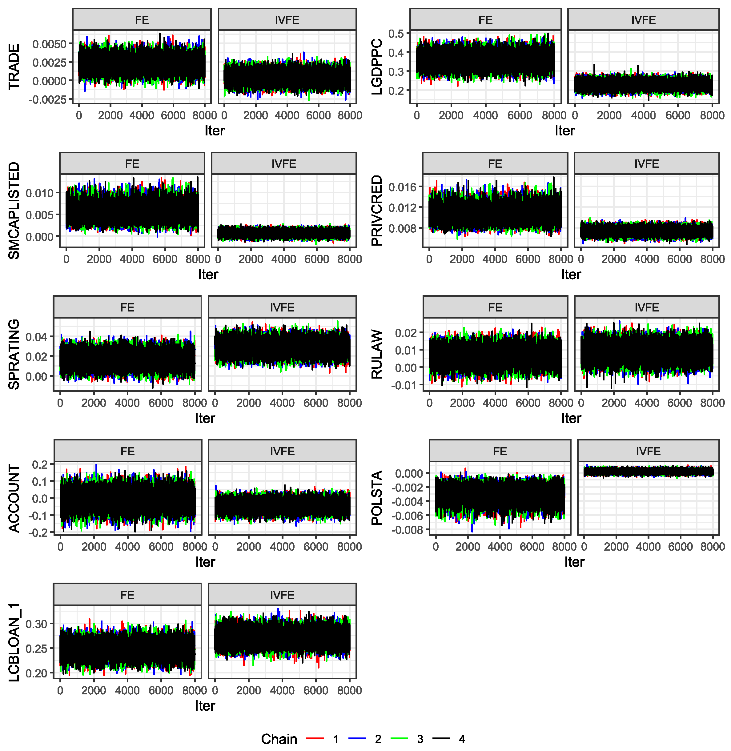
\begin{matrix} \begin{matrix} \begin{matrix} \begin{matrix} \begin{matrix} \begin{matrix} ({\tilde{w}}_{1 i t} | {\tilde{s}}_{1 i t}) ~ N (\sum_{j = 1}^{16} {\tilde{s}}_{1 i t} δ_{j}, σ_{1 \tilde{v}}^{2}); \forall i, t \\ \begin{matrix} ({\tilde{w}}_{2 i t} | {\tilde{s}}_{2 i t}) ~ N (\sum_{j = 1}^{8} {\tilde{s}}_{2 i t} δ_{j}, σ_{2 \tilde{v}}^{2}); \forall i, t \\ ({\tilde{w}}_{3 i t} | {\tilde{s}}_{3 i t}) ~ N (\sum_{j = 1}^{3} {\tilde{s}}_{3 i t} δ_{j}, σ_{3 \tilde{v}}^{2}); \forall i, t \end{matrix} \end{matrix} \\ ({\tilde{y}}_{i t} | {\tilde{y}}_{i, t - 1}, {\tilde{x}}_{i t}^{’}, {\tilde{w}}_{i t}^{’}) ~ N (β_{10} {\tilde{y}}_{i, t - 1} + \sum_{j = 1}^{8} β_{1 j} {\tilde{x}}_{j i t} + \sum_{j = 1}^{3} β_{2 j} {\tilde{w}}_{j i t} + \sum_{j = 1}^{3} β_{3 j} {\tilde{v}}_{j i t}, ω_{11}); \forall i, t \end{matrix} \\ {\tilde{v}}_{l i t} = {\tilde{w}}_{l i t} - \sum_{j} {\tilde{s}}_{l j i t} δ_{l j}; l = 1,2, 3 \end{matrix} \\ (β_{1 j}^{(0)}, β_{2 j}^{(0)}, β_{3 j}^{(0)}) ~ N (0,1); \forall j \end{matrix} \\ σ_{j \tilde{v}}^{2 (0)} ~ I G (2,2); j = 1,2, 3 \end{matrix} \\ ω_{11}^{(0)} ~ I G (2,2) \end{matrix}

(6.4)

We launched four chains of 10,000 iterations each using the NUTS algorithm in STAN, discarding 20% of the first samples as burning. The results are shown in Table 18. Posterior densities and Trace Plots are shown in the Appendix D. The convergence measure,

\hat{R}

, and ESS present reasonable values, and the Monte Carlo standard error (MCSE) is small enough to rely on the results. Results report favourable values for WAIC and BIC model selection criterion to our proposal, therefore, the IVFE model has a better goodness of fit to observed data. In both models, LGDPCC, PRIVCRED, SPRATING, and LCBLOAN_1 are significant variables at the 99% credible level. Variables TRADE and SPRATING was found significant at 95% credibility level in the IVFE model, and variables SMCAPLISTED, POLSTA and GOVEFF were found significant in the IVFE model at 99% credibility level.

Economically, results reported by IVFE model seem to be more consistent with our prior beliefs. TRADE and LGDPPC are both positive in FE and IVFE models, being also significant in the IVFE model, which means that economic cycle plays a positive and relevant partial effect on attracting international bank flows. Internal private credit (PRIVCRED) is significant and positive in both models; therefore, internal private indebtedness acts as a pull factor. In the same way, credit ratings reflect that better trustworthiness of debtors leads to receiving international bank flows. Market Capitalization plays also its positive role in attracting inflows. The main differences arise when comparing country-risk drivers.

Comparing our results with those obtained by Kim and Wu (2008), and accounting for the potential endogeneity in the aforementioned government components, certain observations stand out. In the original study, the variables ACCOUNT and GOVEFF were the only ones with positive signs, indicating that marginal increases in both indicators led to net positive inflows of external banking capital, although only ACCOUNT had a significant estimate. In our estimations, the FE model captures a partial positive effect in the variables RULAW, POLSTA, and GOVEFF, although none of these effects are significant. On the other hand, the IVFE model estimates a positive marginal effect, though not significant, only for the variable RULAW. This finding supports the argument made by (Koepke, 2019) that government indicators are deterrents in attracting external banking flows. Moreover, the IVFE model identifies significant estimates in the variables POLSTA and GOVEFF, effects that are not captured by the FE model. We consider these findings to be economically relevant because both indicators are similar in that they help identify the degree of political stability, its independence, and citizens’ perceptions of the public services provided. Our results also corroborate the idea that foreign banks use a lower perception of the internal development of the private economy to locate financing flows. In fact, the idea that in emerging economies, pressure on the private sector in the form of regulation generates business opportunities for the entry of external bank capital gains strength, in view of our results. Additionally, it’s relevant the fact that IVFE can isolate the relevant partial effect when using governance indicators from those that don’t provide useful added value. In summary, there is some evidence of the positive economic role played by the government sector in attracting foreign bank capital, mainly through the credit rating issued, although the model estimates that an internal capitalized economy is less dependent on foreign financial flows. The combination of good credit quality, along with a favorable development of the private sector of the economy, seems to be a determining factor in the attraction of external bank funds by the emerging economies analyzed.

7. Discussion

In this paper, we propose a general procedure to build instrumental matrices of reduced dimensions in a panel regression model with endogenous explanatory variables. The procedure is based on the collapsed version proposed by Roodman (2009 a, b) and the use of the principal components of instrumental variables, the number of which is selected according to our Bayesian proposal. Our method improves upon existing alternatives by allowing the selection of empirically relevant instruments, preventing issues of multicollinearity among these instruments from causing overfitting in the point estimates of the parameters of interest, while also facilitating the exploration of the sample space due to the orthogonality of the principal components. Once the instrumental matrix has been built, the No-U-Turn sampling algorithm by (Hoffman & Gelman, 2014) is used to make more accurate inferences about the regression coefficients of the endogenous variables. The strengths of our methodology lie in its ability to effectively address endogeneity without sacrificing the desirable statistical properties of the estimators.

Our simulation study robustly demonstrates the effectiveness of the proposed methodology across various scenarios characterized by different degrees of correlation between the endogenous variables and the error terms, as well as varying levels of stationarity. Notably, the results from Table 13, Table 14, Table 15 and Table 16 underscore the robustness of our Bayesian IVFE model in accounting for endogeneity, showing consistent improvements over the traditional fixed effects (FE) model. Across all configurations, including both non-informative and informative priors, and varying sample sizes, the IVFE model provides estimates that are notably closer to the true value, with lower standard errors compared to the FE model. This enhancement in accuracy is particularly evident in the IVFE model’s more precise credible intervals, indicating the model’s reliability in capturing the parameter’s credible range.

Furthermore, we subjected our proposal to a comparative analysis with the widely accepted Difference GMM and System GMM methods in the frequentist community. The results, presented in Table 17, highlight the robust performance of our proposed methodology across diverse scenarios, consistently outperforming the GMM approaches in terms of precision, stability, and reliability of interval estimates. Our model demonstrates a lower standard error in almost every configuration, indicating enhanced accuracy in point estimates under both non-informative and informative prior settings. These findings indicate that our proposal is highly robust and adaptable to diverse data structures, offering a significant advantage over traditional methods in terms of interval stability and precision in point estimates.

The empirical application to the analysis of international bank inflows in emerging economies further underscores the practical utility of our methodology. By accounting for the potential endogeneity of governance indicators, the model yields insights that are more consistent with economic theory and prior expectations. The results suggest that certain governance indicators, such as government effectiveness and political stability, have significant impacts on attracting foreign bank capital—effects that are not captured by models ignoring endogeneity.

While the proposed methodology offers significant improvements over existing approaches, there are avenues for further research that could extend its applicability and effectiveness. One potential direction is to relax some of the initial assumptions regarding the error term properties, such as homoscedasticity and lack of autocorrelation, to accommodate more complex error structures commonly encountered in empirical data. This extension would involve developing methods to handle heteroscedasticity and serial correlation within the Bayesian instrumental variables framework. Another promising area is the exploration of nonlinear relationships and interactions among variables. The assumption of linearity may not hold in all economic contexts, and allowing for nonlinear correlations could provide a more accurate representation of the underlying processes. Moreover, extending the methodology to accommodate high-dimensional data and variable selection techniques could enhance its utility in contemporary econometric applications where the number of potential instruments and regressors is large.

In conclusion, we consider that the proposed methodology represents a significant contribution to addressing endogeneity in dynamic panel data models, especially from a Bayesian perspective. Its robustness, flexibility, and superior performance relative to traditional methods make it a valuable tool for econometric analysis. Future research that expands upon this foundation by relaxing initial assumptions and exploring nonlinear correlations will further enhance its applicability and contribute to the development of more sophisticated econometric models capable of capturing the complexities of real-world data.

Author Contributions

Álvaro Herce (AH) and Manuel Salvador (MS) contributed equally to the development of this paper. AH, as part of his PhD studies, led the conception and design of the study, including the formulation of the Bayesian econometric model and the application of the Monte Carlo Markov Chain (MCMC) methods. He was also responsible for the simulation experiments and the empirical analysis regarding international bank flows. Manuel Salvador contributed to the methodological framework, particularly in the selection of instrumental variables using Principal Component Analysis (PCA). He also provided significant input into the interpretation of the results and the refinement of the final model. Both authors participated in writing and revising the manuscript and approved the final version.

Funding

Not Applicable.

Data Availability Statement

The datasets used and/or analysed during the current study are available from the corresponding author on reasonable request.

Acknowledgments

Not Applicable.

Conflicts of Interest

Declare conflicts of interest or state “The authors declare no conflicts of interest.” Authors must identify and declare any personal circumstances or interest that may be perceived as inappropriately influencing the representation or interpretation of reported research results. Any role of the funders in the design of the study; in the collection, analyses or interpretation of data; in the writing of the manuscript; or in the decision to publish the results must be declared in this section. If there is no role, please state “The funders had no role in the design of the study; in the collection, analyses, or interpretation of data; in the writing of the manuscript; or in the decision to publish the results”.

Appendix A. Deriving Full-Conditional Densities in the Selection of Principal Components

In obtaining the conditional densities used in the development of the Gibbs algorithm for the selection of principal components as valid instruments for instrumental regression, the following developments must be considered, starting from the following specifications:

\begin{matrix} \tilde{w} | \tilde{S}, δ, σ_{\tilde{v}}^{2} ~ N_{N T} (\tilde{S} δ, σ_{\tilde{v}}^{2} I_{N T}) \\ π (σ_{\tilde{v}}^{2}, δ) \propto (\frac{1}{σ_{\tilde{v}}^{2}}) I_{(0, \infty)} (σ_{\tilde{v}}^{2}) \\ p (δ, σ_{\tilde{v}}^{2} | \tilde{w}) \propto {(σ_{\tilde{v}}^{2})}^{- (\frac{N T}{2} + 1)} \exp \{- \frac{1}{2 σ_{\tilde{v}}^{2}} {(\tilde{w} - \tilde{S} δ)}^{’} (\tilde{w} - \tilde{S} δ)\} I_{(0, \infty)} (σ_{\tilde{v}}^{2}) \end{matrix}

Starting from the posterior distribution above, we obtain:

p (σ_{\tilde{v}}^{2} ∣ δ, \tilde{w}) \propto {(σ_{\tilde{v}}^{2})}^{- \{\frac{N T}{2} + 1\}} \exp \{- \frac{{(\tilde{w} - \tilde{S} δ)}^{’} (\tilde{w} - \tilde{S} δ)}{2 σ_{\tilde{v}}^{2}}\} I_{(0, \infty)} (σ_{\tilde{v}}^{2}) \propto {(σ_{\tilde{v}}^{2})}^{- \{a_{1} + 1\}} \exp \{- \frac{b_{1}}{σ_{\tilde{v}}^{2}}\} I_{(0, \infty)} (σ_{\tilde{v}}^{2})

where

\begin{matrix} a_{1} = \frac{N T}{2} \\ b_{1} = \frac{{(\tilde{w} - \tilde{S} δ)}^{’} (\tilde{w} - \tilde{S} δ)}{2} \end{matrix}

The conditional posterior density of the structural parameters

δ

would be:

p (δ ∣ \tilde{w}, σ_{\tilde{v}}^{2}) \propto \exp \{- \frac{1}{2 σ_{\tilde{v}}^{2}} [{(\tilde{w} - \tilde{S} δ)}^{’} (\tilde{w} - \tilde{S} δ)]\} I_{(0, \infty)} (σ_{\tilde{v}}^{2}) \propto \exp \{- \frac{1}{2 σ_{\tilde{v}}^{2}} [δ^{’} {\tilde{S}}^{’} \tilde{S} δ - 2 δ^{’} {\tilde{S}}^{’} \tilde{w}]\} I_{(0, \infty)} (σ_{\tilde{v}}^{2}) \propto \exp \{- \frac{1}{2} [δ^{’} (\frac{1}{σ_{\tilde{v}}^{2}} {\tilde{S}}^{’} \tilde{S}) δ - 2 δ^{’} (\frac{1}{σ_{\tilde{v}}^{2}} {\tilde{S}}^{’} \tilde{S}) σ_{\tilde{v}}^{2} {({\tilde{S}}^{’} \tilde{S})}^{- 1} {\tilde{S}}^{’} \tilde{w}]\} I_{(0, \infty)} (σ_{\tilde{v}}^{2}) \propto \exp \{- \frac{1}{2} [δ^{’} V_{1}^{- 1} δ - 2 δ^{’} V_{1}^{- 1} \hat{δ} + {\hat{δ}}^{’} V_{1}^{- 1} \hat{δ}]\} I_{(0, \infty)} (σ_{\tilde{v}}^{2}) \propto \exp \{- \frac{1}{2} [{(δ - \hat{δ})}^{’} V_{1}^{- 1} (δ - \hat{δ})]\} I_{(0, \infty)} (σ_{\tilde{v}}^{2})

where:

V_{1} = σ_{\tilde{v}}^{2} {({\tilde{S}}^{’} \tilde{S})}^{- 1} \hat{δ} = {({\tilde{S}}^{’} \tilde{S})}^{- 1} {\tilde{S}}^{’} \tilde{w}

This demonstrates that:

σ_{\tilde{v}}^{2} | δ, \tilde{w} ~ I G (a_{1}, b_{1}); a_{1} = \frac{N T}{2}, b_{1} = \frac{{(\tilde{w} - \tilde{S} δ)}^{’} (\tilde{w} - \tilde{S} δ)}{2} δ | σ_{\tilde{v}}^{2}, \tilde{w} ~ N_{K_{\tilde{Z}}} (\hat{δ}, V_{1}); \hat{δ} = {({\tilde{S}}^{’} \tilde{S})}^{- 1} {\tilde{S}}^{’} \tilde{w}, V_{1} = σ_{\tilde{v}}^{2} {({\tilde{S}}^{’} \tilde{S})}^{- 1}

Appendix B. Description of Countries and Applicable Variables

Variable	Description	Obs	Origin
LCBLOAN	Natural log of total loans of BSI reporting banks vis-à-vis individual surveyed countries (in billions of dollars)	1300	BIS, Locational Statistics
TRADE	Percentage of the economy’s GDP of the total value of commercial exchanges	1285	World Bank, WDI
LGDPPC	Natural log of GDP per Capita	1293	World Bank, WDI
SMCAPLISTED	Market capitalization of listed companies, taking the year-end value as a result (% of GDP)	830	World Bank, WDI
PRIVCREDIT	Percentage of credit granted to the private sector as a percentage of GDP	1208	World Bank, Global Financial Development
ACCOUNT	Degree of perception by which a country’s citizens participate in the election of governments, freedom of expression, freedom of association, and freedom of communication	1272	World Bank, Worldwide Governance Indicators
RULAW	Captures citizen’s perception of compliance with the law and social rules	1300	World Bank, Worldwide Governance Indicators
REGQLTY	Captures citizen’s perceptions of the government’s ability to enact and implement sound policies and regulations, to promote private sector development	1300	World Bank, Worldwide Governance Indicators
CORRUPTION	It captures the degree of perception of the power of the public sector to exert pressure on the private sector, including any form of corruption	1300	World Bank, Worldwide Governance Indicators
GOVEFF	Captures the perception of the quality of public services, the quality of civil services and the degree of their independence from public authorities, the quality of policy formulation and its implementation	1300	World Bank, Worldwide Governance Indicators
POLSTA	Measures the perception of the plausibility of political instability and/or political violence, including the possibility of terrorist acts	1300	World Bank, Worldwide Governance Indicators
SPRATING	Long-term credit quality indicator or rating, provided by Standard & Poor’s and denominated in foreign currency	1300	Standard & Poor’s

Appendix C. Posterior Results for Principal Component Search

Table A1. Model with

ρ = 0

and

β_{0} = 0.5 .

Table A1. Model with

ρ = 0

and

β_{0} = 0.5 .

Component	Mean	SD	Q. 2.5	Q. 50	Q. 97.5	ESS	$\hat{R}$
Comp. 1	0.1594***	0.0397	0.0814	0.1596	0.2377	42838	1.0001
Comp. 2	-0.2383***	0.0295	-0.2522	-0.1943	-0.1363	42313	1.0001
Comp. 3	-0.1887***	0.0345	-0.2534	-0.1857	-0.1186	42537	1.0000
Comp. 4	0.1827***	0.0389	-0.2959	-0.2200	-0.1448	42858	1.0001
Comp. 5	-0.1469*	0.0470	-0.3526	-0.2604	-0.1685	42673	1.0001
Comp. 6	-0.0048	0.0561	-0.2518	-0.1402	-0.0314	42701	1.0001
Comp. 7	-0.0037	0.0619	-0.1190	0.0021	0.1251	43031	1.0000
Comp. 8	0.1598	0.0663	-0.1159	0.0131	0.1436	42890	1.0001
Comp. 9	-0.1501	0.0723	-0.0795	0.0603	0.2033	41819	1.0000
*Coefficients marked with () represent significant variables at 90% credible level, () at 95% and () at 99%.*Mean denotes the marginal posterior mean, SE the Square Error, SD the Standard Deviation, Q. 2.5 the 2.5th percentile, Q. 50 the posterior median, and Q. 97.5 the 97.5th percentile. ESS the Effective Sample Size and $\hat{R}$ represents the potential scale reduction factor.

Table A2. Model with

ρ = 0

and

β_{0} = 0.99 .

Table A2. Model with

ρ = 0

and

β_{0} = 0.99 .

Component	Mean	SD	Q. 2.5	Q. 50	Q. 97.5	ESS	$\hat{R}$
Comp. 1	0.1595***	0.0392	0.0821	0.1597	0.2367	40678	1.0001
Comp. 2	-0.2376***	0.0471	-0.3307	-0.2378	-0.1452	42291	1.0000
Comp. 3	-0.1886***	0.0577	-0.3019	-0.1890	-0.0748	41836	1.0000
Comp. 4	0.1826***	0.0675	0.0494	0.1825	0.3155	42361	1.0000
Comp. 5	-0.1464*	0.0794	-0.3006	-0.1463	0.0108	42733	1.0000
Comp. 6	-0.0046	0.0960	-0.1916	-0.0041	0.1842	42562	1.0000
Comp. 7	-0.0048	0.1056	-0.2100	-0.0054	0.2026	42140	1.0000
Comp. 8	0.1613	0.1218	-0.0782	0.1613	0.3997	42528	1.0000
Comp. 9	-0.1517	0.1657	-0.4765	-0.1526	0.1723	42076	1.0001
*Coefficients marked with () represent significant variables at 90% credible level, () at 95% and () at 99%.*Mean denotes the marginal posterior mean, SE the Square Error, SD the Standard Deviation, Q. 2.5 the 2.5th percentile, Q. 50 the posterior median, and Q. 97.5 the 97.5th percentile. ESS the Effective Sample Size and $\hat{R}$ represents the potential scale reduction factor.

Table A3. Model with

ρ = 0.5

and

β_{0} = 0.5 .

Table A3. Model with

ρ = 0.5

and

β_{0} = 0.5 .

Component	Mean	SD	Q. 2.5	Q. 50	Q. 97.5	ESS	$\hat{R}$
Comp. 1	0.1853***	0.0374	0.1122	0.1852	0.2583	42587	1.0000
Comp. 2	-0.2737***	0.0459	-0.3635	-0.2737	-0.1840	42877	1.0000
Comp. 3	-0.2172***	0.0598	-0.3341	-0.2168	-0.1015	41669	1.0001
Comp. 4	-0.1413**	0.0699	-0.2789	-0.1413	-0.0058	42531	1.0000
Comp. 5	0.0496	0.0786	-0.1046	0.0493	0.2036	42408	1.0000
Comp. 6	-0.1665*	0.0939	-0.3485	-0.1671	0.0201	42695	1.0000
Comp. 7	0.1380	0.1113	-0.0791	0.1378	0.3562	42684	1.0000
Comp. 8	-0.1501	0.1234	-0.3924	-0.1499	0.0906	42045	1.0001
Comp. 9	-0.2519	0.1625	-0.5694	-0.2531	0.0670	43016	1.0001
*Coefficients marked with () represent significant variables at 90% credible level, () at 95% and () at 99%.*Mean denotes the marginal posterior mean, SE the Square Error, SD the Standard Deviation, Q. 2.5 the 2.5th percentile, Q. 50 the posterior median, and Q. 97.5 the 97.5th percentile. ESS the Effective Sample Size and $\hat{R}$ represents the potential scale reduction factor.

Table A4. Model with

ρ = 0.5

and

β_{0} = 0.99 .

Table A4. Model with

ρ = 0.5

and

β_{0} = 0.99 .

Component	Mean	SD	Q. 2.5	Q. 50	Q. 97.5	ESS	$\hat{R}$
Comp. 1	0.1854***	0.0377	0.1123	0.1853	0.2596	42417	1.0000
Comp. 2	-0.2741***	0.0457	-0.3639	-0.2741	-0.1845	42835	1.0000
Comp. 3	-0.2176***	0.0598	-0.3339	-0.2178	-0.0995	42007	1.0000
Comp. 4	-0.1417**	0.0701	-0.2799	-0.1413	-0.0039	42690	1.0000
Comp. 5	0.0507	0.0786	-0.1040	0.0505	0.2045	42532	1.0001
Comp. 6	-0.1656*	0.0933	-0.3497	-0.1656	0.0163	42871	1.0000
Comp. 7	0.1374	0.1109	-0.0799	0.1366	0.3544	42747	1.0001
Comp. 8	-0.1496	0.1242	-0.3956	-0.1486	0.0890	42264	1.0000
Comp. 9	-0.2530	0.1629	-0.5734	-0.2524	0.0675	42738	1.0000
*Coefficients marked with () represent significant variables at 90% credible level, () at 95% and () at 99%.*Mean denotes the marginal posterior mean, SE the Square Error, SD the Standard Deviation, Q. 2.5 the 2.5th percentile, Q. 50 the posterior median, and Q. 97.5 the 97.5th percentile. ESS the Effective Sample Size and $\hat{R}$ represents the potential scale reduction factor.

Table A5. Model with

ρ = 0.99

and

β_{0} = 0.5 .

Table A5. Model with

ρ = 0.99

and

β_{0} = 0.5 .

Component	Mean	SD	Q. 2.5	Q. 50	Q. 97.5	ESS	$\hat{R}$
Comp. 1	-0.1681***	0.0402	-0.2471	-0.1682	-0.0892	42439	1.0000
Comp. 2	0.2663***	0.0470	0.1738	0.2662	0.3584	42769	1.0000
Comp. 3	-0.1797***	0.0594	-0.2958	-0.1798	-0.0627	42974	1.0000
Comp. 4	-0.1719**	0.0687	-0.3074	-0.1718	-0.0366	42435	1.0000
Comp. 5	-0.1426*	0.0814	-0.3029	-0.1423	0.0173	42836	1.0000
Comp. 6	0.1588*	0.0897	-0.0159	0.1589	0.3335	42463	1.0000
Comp. 7	0.1228	0.0948	-0.0619	0.1232	0.3093	42454	1.0001
Comp. 8	0.1854*	0.1107	-0.0310	0.1851	0.4044	42945	1.0000
Comp. 9	-0.0186	0.1430	-0.2987	-0.0188	0.2622	42260	1.0000
*Coefficients marked with () represent significant variables at 90% credible level, () at 95% and () at 99%.*Mean denotes the marginal posterior mean, SE the Square Error, SD the Standard Deviation, Q. 2.5 the 2.5th percentile, Q. 50 the posterior median, and Q. 97.5 the 97.5th percentile. ESS the Effective Sample Size and $\hat{R}$ represents the potential scale reduction factor.

Table A6. Model with

ρ = 0.99

and

β_{0} = 0.99 .

Table A6. Model with

ρ = 0.99

and

β_{0} = 0.99 .

Component	Mean	SD	Q. 2.5	Q. 50	Q. 97.5	ESS	$\hat{R}$
Comp. 1	-0.1685***	0.0407	-0.2491	-0.1682	-0.0892	42671	1.0000
Comp. 2	0.2665***	0.0470	0.1745	0.2662	0.3589	42498	1.0000
Comp. 3	-0.1798***	0.0599	-0.2978	-0.1800	-0.0631	42633	1.0000
Comp. 4	-0.1718**	0.0691	-0.3078	-0.1712	-0.0372	42655	1.0000
Comp. 5	-0.1422*	0.0826	-0.3038	-0.1423	0.0202	42618	1.0001
Comp. 6	0.1570*	0.0909	-0.0223	0.1573	0.3331	42474	1.0000
Comp. 7	0.1227	0.0954	-0.0637	0.1227	0.3111	42662	1.0000
Comp. 8	0.1857*	0.1106	-0.0319	0.1858	0.4013	41986	1.0000
Comp. 9	-0.0166	0.1421	-0.2968	-0.0165	0.2618	42511	1.0000
*Coefficients marked with () represent significant variables at 90% credible level, () at 95% and () at 99%.*Mean denotes the marginal posterior mean, SE the Square Error, SD the Standard Deviation, Q. 2.5 the 2.5th percentile, Q. 50 the posterior median, and Q. 97.5 the 97.5th percentile. ESS the Effective Sample Size and $\hat{R}$ represents the potential scale reduction factor.

Table A7. Model with

ρ = 0.99

and

β_{0} = 0.99 . N = 100, T = 10 .

Table A7. Model with

ρ = 0.99

and

β_{0} = 0.99 . N = 100, T = 10 .

Component	Mean	SD	Q. 2.5	Q. 50	Q. 97.5	ESS	$\hat{R}$
Comp. 1	0.2015***	0.0269	0.1488	0.2015	0.2538	42783	1.0000
Comp. 2	0.2168***	0.0349	0.1482	0.2167	0.2856	42474	1.0000
Comp. 3	0.1714***	0.0416	0.0902	0.1713	0.2531	42558	1.0000
Comp. 4	0.1670***	0.0481	0.0729	0.1670	0.2616	42436	1.0001
Comp. 5	-0.0504	0.0545	-0.1568	-0.0505	0.0571	42434	1.0000
Comp. 6	-0.0969	0.0622	-0.2204	-0.0968	0.0244	42587	1.0001
Comp. 7	0.0237	0.0750	-0.1226	0.0234	0.1714	41743	1.0000
Comp. 8	0.1075	0.0802	-0.0500	0.1075	0.2654	42581	1.0001
Comp. 9	-0.0201	0.1041	-0.2231	-0.0196	0.1851	42837	1.0000
*Coefficients marked with () represent significant variables at 90% credible level, () at 95% and () at 99%.*Mean denotes the marginal posterior mean, SE the Square Error, SD the Standard Deviation, Q. 2.5 the 2.5th percentile, Q. 50 the posterior median, and Q. 97.5 the 97.5th percentile. ESS the Effective Sample Size and $\hat{R}$ represents the potential scale reduction factor.

Table A8. Model with

ρ = 0.99

and

β_{0} = 0.99 .

Table A8. Model with

ρ = 0.99

and

β_{0} = 0.99 .

Component	Mean	SD	Q. 2.5	Q. 50	Q. 97.5	ESS	$\hat{R}$
Comp. 1	0.0773***	0.0132	0.0518	0.0772	0.1031	42815	1.0000
Comp. 2	-0.1061***	0.0139	-0.1331	-0.1061	-0.0788	42809	1.0000
Comp. 3	-0.1126***	0.0149	-0.1416	-0.1126	-0.0835	42855	1.0001
Comp. 4	0.0983***	0.0163	0.0664	0.0984	0.1302	42667	1.0000
Comp. 5	0.1215***	0.0168	0.0886	0.1215	0.1544	42537	1.0001
Comp. 6	-0.1205***	0.0182	-0.1564	-0.1204	-0.0850	42783	1.0000
Comp. 7	-0.1076***	0.0191	-0.1450	-0.1076	-0.0699	42173	1.0000
Comp. 8	0.0996***	0.0202	0.0601	0.0996	0.1387	42720	1.0000
Comp. 9	-0.1163***	0.0211	-0.1579	-0.1162	-0.0749	43017	1.0001
Comp. 10	-0.0933***	0.0218	-0.1360	-0.0932	-0.0506	41787	1.0000
Comp. 11	-0.1647***	0.0226	-0.2090	-0.1647	-0.1208	42981	1.0000
Comp. 12	0.1213***	0.0246	0.0730	0.1213	0.1697	42540	1.0000
Comp. 13	-0.1038***	0.0261	-0.1540	-0.1036	-0.0525	43004	1.0000
Comp. 14	0.0812***	0.0267	0.0292	0.0814	0.1334	42698	1.0000
Comp. 15	-0.0992***	0.0275	-0.1536	-0.0992	-0.0456	42744	1.0000
Comp. 16	-0.0798***	0.0284	-0.1351	-0.0800	-0.0238	42945	1.0000
Comp. 17	0.0860***	0.0293	0.0285	0.0860	0.1438	42221	1.0000
Comp. 18	0.0960***	0.0302	0.0374	0.0960	0.1555	42496	1.0000
Comp. 19	0.0597*	0.0310	-0.0004	0.0595	0.1205	42585	1.0000
Comp. 20	-0.0660**	0.0317	-0.1280	-0.0660	-0.0036	42719	1.0000
Comp. 21	-0.0574*	0.0326	-0.1222	-0.0573	0.0066	42727	1.0001
Comp. 22	0.0055	0.0339	-0.0604	0.0055	0.0721	42128	1.0000
Comp. 23	0.0256	0.0341	-0.0413	0.0256	0.0925	42648	1.0000
Comp. 24	0.0815**	0.0346	0.0138	0.0819	0.1492	42722	1.0000
Comp. 25	0.0385	0.0361	-0.0326	0.0387	0.1088	42547	1.0000
Comp. 26	-0.0475	0.0366	-0.1195	-0.0475	0.0244	42903	1.0000
Comp. 27	-0.0694*	0.0373	-0.1422	-0.0697	0.0041	42860	1.0000
Comp. 28	-0.0255	0.0388	-0.1004	-0.0255	0.0508	42599	1.0001
Comp. 29	0.0171	0.0395	-0.0601	0.0173	0.0945	42527	1.0000
Comp. 30	-0.0574	0.0413	-0.1384	-0.0573	0.0249	42748	1.0001
Comp. 31	0.0194	0.0431	-0.0655	0.0197	0.1028	42750	1.0001
Comp. 32	-0.0029	0.0440	-0.0894	-0.0029	0.0834	42679	1.0000
Comp. 33	0.0641	0.0463	-0.0251	0.0643	0.1543	42526	1.0000
Comp. 34	0.0347	0.0476	-0.0588	0.0350	0.1276	42283	1.0001
Comp. 35	0.0206	0.0496	-0.0767	0.0202	0.1183	42961	1.0000
Comp. 36	0.0452	0.0504	-0.0533	0.0453	0.1442	42786	1.0000
Comp. 37	-0.0651	0.0522	-0.1671	-0.0651	0.0373	42393	1.0000
Comp. 38	-0.0375	0.0541	-0.1438	-0.0372	0.0687	42655	1.0000
Comp. 39	0.0049	0.0562	-0.1052	0.0048	0.1148	42356	1.0001
Comp. 40	0.0177	0.0598	-0.0988	0.0177	0.1342	42650	1.0000
Comp. 41	-0.0511	0.0621	-0.1723	-0.0509	0.0716	42645	1.0000
Comp. 42	-0.0112	0.0649	-0.1387	-0.0110	0.1174	42532	1.0000
Comp. 43	-0.0978	0.0698	-0.2350	-0.0981	0.0394	42450	1.0001
Comp. 44	-0.0860	0.0744	-0.2304	-0.0859	0.0591	42417	1.0001
Comp. 45	0.0164	0.0821	-0.1446	0.0169	0.1768	42635	1.0000
Comp. 46	-0.0517	0.0893	-0.2259	-0.0515	0.1235	42123	1.0001
Comp. 47	0.1067	0.1011	-0.0912	0.1071	0.3031	42533	1.0000
Comp. 48	0.0029	0.1276	-0.2461	0.0024	0.2512	42300	1.0000
Comp. 49	-0.0830	0.1631	-0.4009	-0.0833	0.2363	42471	1.0001
*Coefficients marked with () represent significant variables at 90% credible level, () at 95% and () at 99%.*Mean denotes the marginal posterior mean, SE the Square Error, SD the Standard Deviation, Q. 2.5 the 2.5th percentile, Q. 50 the posterior median, and Q. 97.5 the 97.5th percentile. ESS the Effective Sample Size and $\hat{R}$ represents the potential scale reduction factor.

Appendix D. Posterior Densities and Trace Plots for the Parameters of the Empirical Application

Figure A1. Posterior densities for endogenous variables.

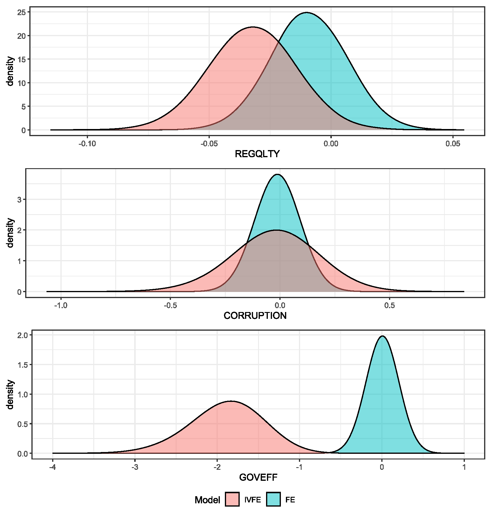
Figure A2. Posterior densities for endogenous variables.

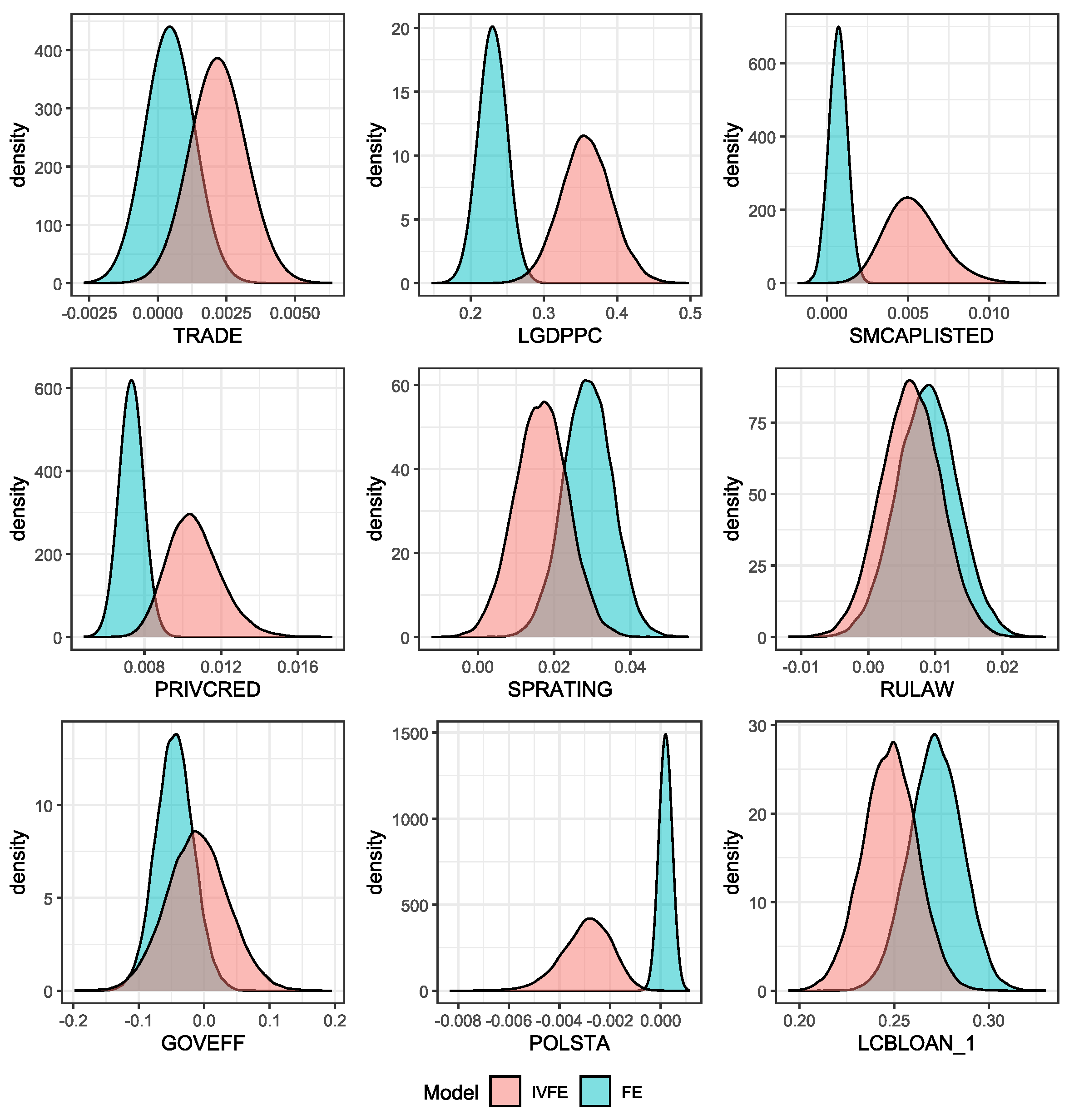
Figure A3. Trace plot for endogenous variables.

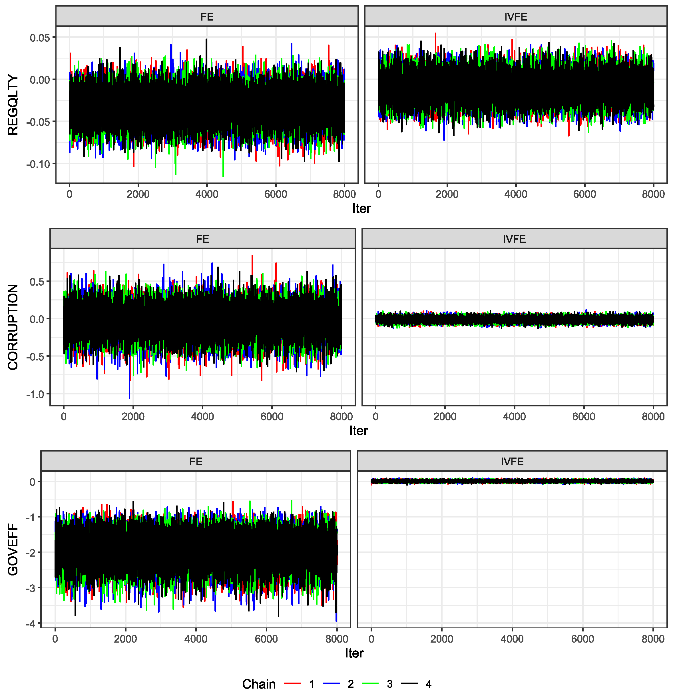
Figure A4. Trace plot for exogenous variables.

References

Arellano, M., & Bond, S. (1991). Some tests of specification for panel data: Monte Carlo evidence and an application to employment equations. The Review of Economic Studies, 58(2), 277–297. [CrossRef]
Arellano, M., & Bover, O. (1995). Another look at the instrumental variable estimation of error-components models. Journal of Econometrics, 68(1), 29–51. [CrossRef]
Blundell, R., & Bond, S. (1998). Initial conditions and moment restrictions in dynamic panel data models. Journal of Econometrics, 87(1), 115–143. [CrossRef]
Carpenter, B., Gelman, A., Hoffman, M. D., Lee, D., Goodrich, B., Betancourt, M., Brubaker, M. A., Guo, J., Li, P., & Riddell, A. (2017). Stan: A probabilistic programming language. Journal of Statistical Software, 76. [CrossRef]
Chib, S. (2008). Panel data modeling and inference: A Bayesian primer. In The econometrics of panel data: Fundamentals and recent developments in theory and practice (pp. 479–515). Springer. [CrossRef]
Croissant, Y., & Millo, G. (2019). Panel data econometrics with R. Wiley Online Library.
Gelman, A., Carlin, J. B., Stern, H. S., & Rubin, D. B. (2014). Bayesian data analysis. Chapman and Hall/CRC.
Geman, S., & Geman, D. (1984). Stochastic relaxation, Gibbs distributions, and the Bayesian restoration of images. IEEE Transactions on Pattern Analysis and Machine Intelligence, 6, 721–741. [CrossRef]
Greenberg, E. (2012). Introduction to Bayesian econometrics. Cambridge University Press.
Hadi, A. S., & Ling, R. F. (1998). Some cautionary notes on the use of principal components regression. The American Statistician, 52(1), 15–19. [CrossRef]
Hoffman, M. D., & Gelman, A. (2014). The No-U-Turn sampler: Adaptively setting path lengths in Hamiltonian Monte Carlo. J. Mach. Learn. Res., 15(1), 1593–1623.
Holtz-Eakin, D., Newey, W., & Rosen, H. S. (1988). Estimating vector autoregressions with panel data. Econometrica: Journal of the Econometric Society, 1371–1395. [CrossRef]
Jeffreys, H. (1961). The theory of probability (3rd ed.). Clarendon Press, Oxford.
Jolliffe, I. T. (1982). A note on the use of principal components in regression. Journal of the Royal Statistical Society Series C: Applied Statistics, 31(3), 300–303. [CrossRef]
Kim, S.-J., & Wu, E. (2008). Sovereign credit ratings, capital flows and financial sector development in emerging markets. Emerging Markets Review, 9(1), 17–39. [CrossRef]
Koepke, R. (2019). What Drives Capital Flows to Emerging Markets? A Survey of the Empirical Literature. Journal of Economic Surveys, 33(2), 516–540. [CrossRef]
Mátyás, L., & Sevestre, P. (2008). The econometrics of panel data: Fundamentals and recent developments in theory and practice.
Nickell, S. (1981). Biases in dynamic models with fixed effects. Econometrica: Journal of the Econometric Society, 1417–1426. [CrossRef]
Roodman, D. (2009a). A Note on the Theme of Too Many Instruments. Oxford Bulletin of Economics and Statistics, 71(1), 135–158. [CrossRef]
Roodman, D. (2009b). How to do xtabond2: An introduction to difference and system GMM in Stata. The Stata Journal, 9(1), 86–136. [CrossRef]

Table 1. Non-Informative prior with

ρ = 0

and

β_{0}

= 0.5.

Table 1. Non-Informative prior with

ρ = 0

and

β_{0}

= 0.5.

Variable	Real	Mean		SE		SD		Q. 2.5		Q. 50		Q. 97.5		ESS		$\hat{R}$
		FE	IVFE	FE	IVFE	FE	IVFE	FE	IVFE	FE	IVFE	FE	IVFE	FE	IVFE	FE	IVFE
$β_{0}$	0.5	0.4784	0.4839	0.0005	0.0003	0.0154	0.0188	0.4482	0.4466	0.4784	0.4839	0.5085	0.5209	36307	19163	1.0000	1.0000
$β_{1}$	3	2.9865	2.9879	0.0002	0.0001	0.1008	0.1003	2.7893	2.7895	2.9861	2.9879	3.1834	3.1834	35749	34508	1.0000	1.0000
$β_{2}$	2	2.1054	2.0273	0.0111	0.0007	0.0452	0.1509	2.0172	1.7303	2.1053	2.0269	2.1948	2.3255	35779	12682	1.0000	1.0000
WAIC:		1949.40	1951.10
BIC:		1963.35	1963.96
Five Principal Components employed: PC1, PC2, PC3, PC4, PC5. We refer to FE as a model without endogeneity treatment, while IVFE denotes a model that incorporates our proposal. Mean denotes the marginal posterior mean, SE the Square Error, SD the Standard Deviation, Q. 2.5 the 2.5th percentile, Q. 50 the posterior median, and Q. 97.5 the 97.5th percentile. ESS the Effective Sample Size and R ̂ represents the potential scale reduction factor.

Table 2. Non-Informative prior with

ρ = 0

and

β_{0} = 0.99 .

Table 2. Non-Informative prior with

ρ = 0

and

β_{0} = 0.99 .

Variable	Real	Mean		SE		SD		Q. 2.5		Q. 50		Q. 97.5		ESS		$\hat{R}$
		FE	IVFE	FE	IVFE	FE	IVFE	FE	IVFE	FE	IVFE	FE	IVFE	FE	IVFE	FE	IVFE
$β_{0}$	0.99	0.9766	0.9787	0.0002	0.0001	0.0100	0.0102	0.9572	0.9588	0.9766	0.9786	0.9964	0.9985	34575	48222	1.0000	1.0000
$β_{1}$	3	2.9810	2.9810	0.0004	0.0004	0.1010	0.1014	2.7823	2.7809	2.9807	2.9813	3.1785	3.1804	34322	53894	1.0000	0.9999
$β_{2}$	2	2.0896	1.9738	0.0080	0.0007	0.0450	0.1268	2.0016	1.7166	2.0896	1.9761	2.1777	2.2180	32342	22718	1.0001	1.0000
WAIC:		1949.50	1950.60
BIC:		1963.51	1963.45
Five Principal Components employed: PC1, PC2, PC3, PC4, PC5. We refer to FE as a model without endogeneity treatment, while IVFE denotes a model that incorporates our proposal. Mean denotes the marginal posterior mean, SE the Square Error, SD the Standard Deviation, Q. 2.5 the 2.5th percentile, Q. 50 the posterior median, and Q. 97.5 the 97.5th percentile. ESS the Effective Sample Size and R ̂ represents the potential scale reduction factor.

Table 3. Non-Informative prior with

ρ = 0.5

and

β_{0} = 0.5 .

Table 3. Non-Informative prior with

ρ = 0.5

and

β_{0} = 0.5 .

Variable	Real	Mean		SE		SD		Q. 2.5		Q. 50		Q. 97.5		ESS		$\hat{R}$
		FE	IVFE	FE	IVFE	FE	IVFE	FE	IVFE	FE	IVFE	FE	IVFE	FE	IVFE	FE	IVFE
$β_{0}$	0.5	0.4342	0.4497	0.3089	0.2919	0.0140	0.0189	0.4069	0.4131	0.4342	0.4496	0.4619	0.4870	31700	19411	1.0000	1.0002
$β_{1}$	3	2.9732	2.9645	0.0007	0.0013	0.1024	0.1030	2.7710	2.7630	2.9734	2.9642	3.1745	3.1668	33821	40723	1.0000	1.0000
$β_{2}$	2	2.4325	2.2581	0.1871	0.0666	0.0455	0.1495	2.3442	1.9596	2.4320	2.2610	2.5217	2.5463	31605	14760	0.9999	1.0001
WAIC:		1973.60	1974.10
BIC:		1987.37	1986.77
Five Principal Components employed: PC1, PC2, PC3, PC4, PC6. We refer to FE as a model without endogeneity treatment, while IVFE denotes a model that incorporates our proposal. Mean denotes the marginal posterior mean, SE the Square Error, SD the Standard Deviation, Q. 2.5 the 2.5th percentile, Q. 50 the posterior median, and Q. 97.5 the 97.5th percentile. ESS the Effective Sample Size and R ̂ represents the potential scale reduction factor.

Table 4. Non-Informative prior with

ρ = 0.5

and

β_{0} = 0.99 .

Table 4. Non-Informative prior with

ρ = 0.5

and

β_{0} = 0.99 .

Variable	Real	Mean		SE		SD		Q. 2.5		Q. 50		Q. 97.5		ESS		$\hat{R}$
		FE	IVFE	FE	IVFE	FE	IVFE	FE	IVFE	FE	IVFE	FE	IVFE	FE	IVFE	FE	IVFE
$β_{0}$	0.99	0.9589	0.9673	0.0010	0.0005	0.0090	0.0094	0.9413	0.9489	0.9588	0.9673	0.9766	0.9858	40020	48536	0.9999	0.9999
$β_{1}$	3	2.9712	2.9474	0.0008	0.0028	0.1046	0.1035	2.7655	2.7457	2.9711	2.9477	3.1757	3.1511	40297	55340	1.0000	0.9999
$β_{2}$	2	2.3670	2.0433	0.1347	0.0019	0.0457	0.1190	2.2780	1.7982	2.3667	2.0474	2.4570	2.2646	37308	24002	0.9999	1.0000
WAIC:		1983.50	1975.50
BIC:		1997.44	1987.89
Five Principal Components employed: PC1, PC2, PC3, PC4, PC6. We refer to FE as a model without endogeneity treatment, while IVFE denotes a model that incorporates our proposal. Mean denotes the marginal posterior mean, SE the Square Error, SD the Standard Deviation, Q. 2.5 the 2.5th percentile, Q. 50 the posterior median, and Q. 97.5 the 97.5th percentile. ESS the Effective Sample Size and R ̂ represents the potential scale reduction factor.

Table 5. Non-Informative prior with

ρ = 0.99

and

β_{0} = 0.5 .

Table 5. Non-Informative prior with

ρ = 0.99

and

β_{0} = 0.5 .

Variable	Real	Mean		SE		SD		Q. 2.5		Q. 50		Q. 97.5		ESS		$\hat{R}$
		FE	IVFE	FE	IVFE	FE	IVFE	FE	IVFE	FE	IVFE	FE	IVFE	FE	IVFE	FE	IVFE
$β_{0}$	0.5	0.4203	0.4575	0.3246	0.2836	0.0088	0.0126	0.4030	0.4334	0.4202	0.4573	0.4376	0.4827	36504	20811	1.0000	1.0001
$β_{1}$	3	3.0558	3.1173	0.0031	0.0138	0.0590	0.0754	2.9386	2.9729	3.0561	3.1162	3.1710	3.2682	33615	23064	1.0000	1.0001
$β_{2}$	2	2.6731	2.1566	0.4531	0.0245	0.0315	0.1303	2.6115	1.8730	2.6731	2.1661	2.7346	2.3862	34020	13410	1.0000	1.0001
WAIC:		1499.80	1473.80
BIC:		1514.24	1485.11
Seven Principal Components employed: PC1, PC2, PC3, PC4, PC5, PC6, PC8. We refer to FE as a model without endogeneity treatment, while IVFE denotes a model that incorporates our proposal. Mean denotes the marginal posterior mean, SE the Square Error, SD the Standard Deviation, Q. 2.5 the 2.5th percentile, Q. 50 the posterior median, and Q. 97.5 the 97.5th percentile. ESS the Effective Sample Size and R ̂ represents the potential scale reduction factor.

Table 6. Non-Informative prior with

ρ = 0.99

and

β_{0} = 0.99 .

Table 6. Non-Informative prior with

ρ = 0.99

and

β_{0} = 0.99 .

Variable	Real	Mean		SE		SD		Q. 2.5		Q. 50		Q. 97.5		ESS		$\hat{R}$
		FE	IVFE	FE	IVFE	FE	IVFE	FE	IVFE	FE	IVFE	FE	IVFE	FE	IVFE	FE	IVFE
$β_{0}$	0.99	0.9516	0.9676	0.0015	0.0005	0.0065	0.0067	0.9389	0.9545	0.9516	0.9675	0.9644	0.9808	31519	27570	1.0000	1.0001
$β_{1}$	3	3.0394	3.1109	0.0016	0.0123	0.0628	0.0852	2.9157	2.9440	3.0395	3.1105	3.1625	3.2803	34416	17941	1.0000	1.0000
$β_{2}$	2	2.5922	1.9474	0.3507	0.0028	0.0329	0.1213	2.5280	1.6825	2.5922	1.9575	2.6560	2.1564	29012	9867	1.0000	1.0004
WAIC:		1541.90	1471.70
BIC:		1556.13	1482.12
Seven Principal Components employed: PC1, PC2, PC3, PC4, PC5, PC6, PC8. We refer to FE as a model without endogeneity treatment, while IVFE denotes a model that incorporates our proposal. Mean denotes the marginal posterior mean, SE the Square Error, SD the Standard Deviation, Q. 2.5 the 2.5th percentile, Q. 50 the posterior median, and Q. 97.5 the 97.5th percentile. ESS the Effective Sample Size and R ̂ represents the potential scale reduction factor.

Table 7. Informative prior with

ρ = 0

and

β_{0} = 0.5 .

Table 7. Informative prior with

ρ = 0

and

β_{0} = 0.5 .

Variable	Real	Mean		SE		SD		Q. 2.5		Q. 50		Q. 97.5		ESS		$\hat{R}$
		FE	IVFE	FE	IVFE	FE	IVFE	FE	IVFE	FE	IVFE	FE	IVFE	FE	IVFE	FE	IVFE
$β_{0}$	0.5	0.4781	0.4864	0.0005	0.0002	0.0153	0.0185	0.4481	0.4502	0.4781	0.4864	0.5080	0.5226	35334	21534	1.0000	1.0000
$β_{1}$	3	2.9578	2.9593	0.0018	0.0017	0.0994	0.0994	2.7613	2.7658	2.9577	2.9590	3.1521	3.1543	34792	39588	0.9999	1.0000
$β_{2}$	2	2.1017	1.9849	0.0103	0.0002	0.0450	0.1486	2.0136	1.6844	2.1018	1.9863	2.1912	2.2729	33335	14394	0.9999	1.0001
WAIC:		1949.50	1951.20
BIC:		1963.41	1964.02
Five Principal Components employed: PC1, PC2, PC3, PC4, PC5. We refer to FE as a model without endogeneity treatment, while IVFE denotes a model that incorporates our proposal. Mean denotes the marginal posterior mean, SE the Square Error, SD the Standard Deviation, Q. 2.5 the 2.5th percentile, Q. 50 the posterior median, and Q. 97.5 the 97.5th percentile. ESS the Effective Sample Size and R ̂ represents the potential scale reduction factor.

Table 8. Informative prior with

ρ = 0

and

β_{0} = 0.99 .

Table 8. Informative prior with

ρ = 0

and

β_{0} = 0.99 .

Variable	Real	Mean		SE		SD		Q. 2.5		Q. 50		Q. 97.5		ESS		$\hat{R}$
		FE	IVFE	FE	IVFE	FE	IVFE	FE	IVFE	FE	IVFE	FE	IVFE	FE	IVFE	FE	IVFE
$β_{0}$	0.99	0.9759	0.9786	0.0002	0.0001	0.0100	0.0104	0.9563	0.9581	0.9759	0.9786	0.9956	0.9987	35163	52038	1.0000	0.9999
$β_{1}$	3	2.9512	2.9513	0.0024	0.0024	0.1005	0.0986	2.7552	2.7583	2.9508	2.9513	3.1491	3.1459	36351	52844	1.0000	0.9999
$β_{2}$	2	2.0848	1.9468	0.0072	0.0028	0.0455	0.1245	1.9961	1.6936	2.0848	1.9497	2.1747	2.1873	33226	24286	1.0001	1.0001
WAIC:		1949.70	1950.50
BIC:		1963.61	1963.45
Five Principal Components employed: PC1, PC2, PC3, PC4, PC5. We refer to FE as a model without endogeneity treatment, while IVFE denotes a model that incorporates our proposal. Mean denotes the marginal posterior mean, SE the Square Error, SD the Standard Deviation, Q. 2.5 the 2.5th percentile, Q. 50 the posterior median, and Q. 97.5 the 97.5th percentile. ESS the Effective Sample Size and R ̂ represents the potential scale reduction factor.

Table 9. Informative prior with

ρ = 0.5

and

β_{0} = 0.5 .

Table 9. Informative prior with

ρ = 0.5

and

β_{0} = 0.5 .

Variable	Real	Mean		SE		SD		Q. 2.5		Q. 50		Q. 97.5		ESS		$\hat{R}$
		FE	IVFE	FE	IVFE	FE	IVFE	FE	IVFE	FE	IVFE	FE	IVFE	FE	IVFE	FE	IVFE
$β_{0}$	0.5	0.4341	0.4532	0.3090	0.2882	0.0139	0.0188	0.4066	0.4164	0.4341	0.4531	0.4613	0.4908	31337	17322	1.0000	1.0002
$β_{1}$	3	2.9420	2.9315	0.0034	0.0047	0.1014	0.1030	2.7430	2.7293	2.9422	2.9316	3.1412	3.1318	34179	35815	1.0000	1.0000
$β_{2}$	2	2.4281	2.2107	0.1833	0.0444	0.0450	0.1503	2.3407	1.9053	2.4279	2.2133	2.5165	2.4945	34175	13103	0.9999	1.0001
WAIC:		1973.60	1974.30
BIC:		1987.42	1986.90
Five Principal Components employed: PC1, PC2, PC3, PC4, PC6. We refer to FE as a model without endogeneity treatment, while IVFE denotes a model that incorporates our proposal. Mean denotes the marginal posterior mean, SE the Square Error, SD the Standard Deviation, Q. 2.5 the 2.5th percentile, Q. 50 the posterior median, and Q. 97.5 the 97.5th percentile. ESS the Effective Sample Size and R ̂ represents the potential scale reduction factor.

Table 10. Informative prior with

ρ = 0.5

and

β_{0} = 0.99 .

Table 10. Informative prior with

ρ = 0.5

and

β_{0} = 0.99 .

Variable	Real	Mean		SE		SD		Q. 2.5		Q. 50		Q. 97.5		ESS		$\hat{R}$
		FE	IVFE	FE	IVFE	FE	IVFE	FE	IVFE	FE	IVFE	FE	IVFE	FE	IVFE	FE	IVFE
$β_{0}$	0.99	0.9584	0.9672	0.0010	0.0005	0.0090	0.0093	0.9409	0.9489	0.9584	0.9672	0.9759	0.9854	33655	46481	0.9999	1.0000
$β_{1}$	3	2.9393	2.9143	0.0037	0.0073	0.1025	0.1032	2.7374	2.7120	2.9395	2.9141	3.1409	3.1153	34386	54883	1.0000	0.9999
$β_{2}$	2	2.3627	2.0180	0.1316	0.0003	0.0452	0.1193	2.2747	1.7698	2.3628	2.0222	2.4518	2.2417	31974	21565	0.9999	1.0001
WAIC:		1983.50	1975.50
BIC:		1997.48	1987.91
Five Principal Components employed: PC1, PC2, PC3, PC4, PC6. We refer to FE as a model without endogeneity treatment, while IVFE denotes a model that incorporates our proposal. Mean denotes the marginal posterior mean, SE the Square Error, SD the Standard Deviation, Q. 2.5 the 2.5th percentile, Q. 50 the posterior median, and Q. 97.5 the 97.5th percentile. ESS the Effective Sample Size and R ̂ represents the potential scale reduction factor.

Table 11. Informative prior with

ρ = 0.99

and

β_{0} = 0.5 .

Table 11. Informative prior with

ρ = 0.99

and

β_{0} = 0.5 .

Variable	Real	Mean		SE		SD		Q. 2.5		Q. 50		Q. 97.5		ESS		$\hat{R}$
		FE	IVFE	FE	IVFE	FE	IVFE	FE	IVFE	FE	IVFE	FE	IVFE	FE	IVFE	FE	IVFE
$β_{0}$	0.5	0.4201	0.4587	0.3248	0.2823	0.0088	0.0126	0.4026	0.4345	0.4200	0.4585	0.4373	0.4839	35365	16931	1.0000	1.0003
$β_{1}$	3	3.0454	3.1019	0.0021	0.0104	0.0590	0.0760	2.9296	2.9540	3.0456	3.1008	3.1617	3.2544	31727	21408	0.9999	0.9999
$β_{2}$	2	2.6710	2.1311	0.4502	0.0172	0.0315	0.1347	2.6092	1.8352	2.6711	2.1409	2.7332	2.3680	33320	10440	1.0001	1.0004
WAIC:		1499.80	1473.60
BIC:		1514.28	1484.84
Seven Principal Components employed: PC1, PC2, PC3, PC4, PC5, PC6, PC8. We refer to FE as a model without endogeneity treatment, while IVFE denotes a model that incorporates our proposal. Mean denotes the marginal posterior mean, SE the Square Error, SD the Standard Deviation, Q. 2.5 the 2.5th percentile, Q. 50 the posterior median, and Q. 97.5 the 97.5th percentile. ESS the Effective Sample Size and R ̂ represents the potential scale reduction factor.

Table 12. Informative prior with

ρ = 0.99

and

β_{0} = 0.99 .

Table 12. Informative prior with

ρ = 0.99

and

β_{0} = 0.99 .

Variable	Real	Mean		SE		SD		Q. 2.5		Q. 50		Q. 97.5		ESS		$\hat{R}$
		FE	IVFE	FE	IVFE	FE	IVFE	FE	IVFE	FE	IVFE	FE	IVFE	FE	IVFE	FE	IVFE
$β_{0}$	0.99	0.9511	0.9676	0.0015	0.0005	0.0066	0.0067	0.9381	0.9545	0.9512	0.9675	0.9639	0.9808	34135	27570	1.0001	1.0001
$β_{1}$	3	3.0268	3.1109	0.0007	0.0123	0.0620	0.0852	2.9051	2.9440	3.0266	3.1105	3.1495	3.2803	30983	17941	0.9999	1.0000
$β_{2}$	2	2.5893	1.9474	0.3473	0.0028	0.0334	0.1213	2.5243	1.6825	2.5893	1.9575	2.6551	2.1564	30185	9867	1.0001	1.0004
WAIC:		1541.90	1471.50
BIC:		1556.18	1481.97
Seven Principal Components employed: PC1, PC2, PC3, PC4, PC5, PC6, PC8. We refer to FE as a model without endogeneity treatment, while IVFE denotes a model that incorporates our proposal. Mean denotes the marginal posterior mean, SE the Square Error, SD the Standard Deviation, Q. 2.5 the 2.5th percentile, Q. 50 the posterior median, and Q. 97.5 the 97.5th percentile. ESS the Effective Sample Size and R ̂ represents the potential scale reduction factor.

Table 13. Non-Informative prior with

ρ = 0.99

and

β_{0} = 0.99

. N = 100, T = 10.

Table 13. Non-Informative prior with

ρ = 0.99

and

β_{0} = 0.99

. N = 100, T = 10.

Variable	Real	Mean		SE		SD		Q. 2.5		Q. 50		Q. 97.5		ESS		$\hat{R}$
		FE	IVFE	FE	IVFE	FE	IVFE	FE	IVFE	FE	IVFE	FE	IVFE	FE	IVFE	FE	IVFE
$β_{0}$	0.99	0.9704	0.9812	0.0004	0.0001	0.0038	0.0038	0.9630	0.9736	0.9704	0.9812	0.9779	0.9886	38016	39053	0.9999	1.0000
$β_{1}$	3	2.9992	3.0200	0.0000	0.0004	0.0461	0.0439	2.9098	2.9338	2.9990	3.0198	3.0893	3.1053	32305	32228	0.9999	0.9999
$β_{2}$	2	2.3827	1.9112	0.1465	0.0079	0.0193	0.0692	2.3449	1.7643	2.3826	1.9150	2.4207	2.0373	30176	10868	0.9999	1.0001
WAIC:		3114.40	3024.70
BIC:		3130.78	3038.99
Four Principal Components employed: PC1, PC2, PC3, PC4. We refer to FE as a model without endogeneity treatment, while IVFE denotes a model that incorporates our proposal. Mean denotes the marginal posterior mean, SE the Square Error, SD the Standard Deviation, Q. 2.5 the 2.5th percentile, Q. 50 the posterior median, and Q. 97.5 the 97.5th percentile. ESS the Effective Sample Size and R ̂ represents the potential scale reduction factor.

Table 14. Informative prior with

ρ = 0.99

and

β_{0} = 0.99

. N = 100, T = 10.

Table 14. Informative prior with

ρ = 0.99

and

β_{0} = 0.99

. N = 100, T = 10.

Variable	Real	Mean		SE		SD		Q. 2.5		Q. 50		Q. 97.5		ESS		$\hat{R}$
		FE	IVFE	FE	IVFE	FE	IVFE	FE	IVFE	FE	IVFE	FE	IVFE	FE	IVFE	FE	IVFE
$β_{0}$	0.99	0.9703	0.9811	0.0004	0.0001	0.0038	0.0038	0.9629	0.9736	0.9703	0.9812	0.9777	0.9887	39665	32669	1.0000	1.0000
$β_{1}$	3	2.9935	3.0147	0.0000	0.0002	0.0458	0.0438	2.9050	2.9295	2.9934	3.0143	3.0825	3.1014	33731	29637	0.9999	1.0000
$β_{2}$	2	2.3818	1.9044	0.1458	0.0091	0.0194	0.0706	2.3435	1.7534	2.3817	1.9084	2.4201	2.0317	32535	11914	1.0002	1.0001
WAIC:		3144.40	3024.90
BIC:		3130.80	3039.07
Four Principal Components employed: PC1, PC2, PC3, PC4. We refer to FE as a model without endogeneity treatment, while IVFE denotes a model that incorporates our proposal. Mean denotes the marginal posterior mean, SE the Square Error, SD the Standard Deviation, Q. 2.5 the 2.5th percentile, Q. 50 the posterior median, and Q. 97.5 the 97.5th percentile. ESS the Effective Sample Size and R ̂ represents the potential scale reduction factor.

Table 15. Non-Informative prior with

ρ = 0.99

and

β_{0} = 0.99

. N = 50, T = 50.

Table 15. Non-Informative prior with

ρ = 0.99

and

β_{0} = 0.99

. N = 50, T = 50.

Variable	Real	Mean		SE		SD		Q. 2.5		Q. 50		Q. 97.5		ESS		$\hat{R}$
		FE	IVFE	FE	IVFE	FE	IVFE	FE	IVFE	FE	IVFE	FE	IVFE	FE	IVFE	FE	IVFE
$β_{0}$	0.99	0.9817	0.9869	0.0001	0.0000	0.0013	0.0013	0.9791	0.9843	0.9817	0.9869	0.9842	0.9895	42535	37297	0.9999	1.0000
$β_{1}$	3	2.9681	2.9553	0.0010	0.0020	0.0315	0.0291	2.9063	2.8987	2.9682	2.9554	3.0298	3.0128	28576	73372	1.0000	0.9999
$β_{2}$	2	2.4895	2.0466	0.2396	0.0022	0.0129	0.0335	2.4643	1.9783	2.4895	2.0473	2.5147	2.1100	28485	19806	0.9999	1.0000
WAIC:		9117.70	8766.80
BIC:		9137.11	8775.98
Twenty-three Principal Components employed: PC1-PC21, PC24, PC27. We refer to FE as a model without endogeneity treatment, while IVFE denotes a model that incorporates our proposal. Mean denotes the marginal posterior mean, SE the Square Error, SD the Standard Deviation, Q. 2.5 the 2.5th percentile, Q. 50 the posterior median, and Q. 97.5 the 97.5th percentile. ESS the Effective Sample Size and R ̂ represents the potential scale reduction factor.

Table 16. Informative prior with

ρ = 0.99

and

β_{0} = 0.99

. N = 50, T = 50.

Table 16. Informative prior with

ρ = 0.99

and

β_{0} = 0.99

. N = 50, T = 50.

Variable	Real	Mean		SE		SD		Q. 2.5		Q. 50		Q. 97.5		ESS		$\hat{R}$
		FE	IVFE	FE	IVFE	FE	IVFE	FE	IVFE	FE	IVFE	FE	IVFE	FE	IVFE	FE	IVFE
$β_{0}$	0.99	0.9817	0.9869	0.0001	0.0000	0.0013	0.0013	0.9791	0.9843	0.9817	0.9869	0.9842	0.9895	42535	37297	0.9999	1.0000
$β_{1}$	3	2.9681	2.9553	0.0010	0.0020	0.0315	0.0291	2.9063	2.8987	2.9682	2.9554	3.0298	3.0128	28576	73372	1.0000	0.9999
$β_{2}$	2	2.4895	2.0466	0.2396	0.0022	0.0129	0.0335	2.4643	1.9783	2.4895	2.0473	2.5147	2.1100	28485	19806	0.9999	1.0000
WAIC:		9117.70	8766.80
BIC:		9137.11	8775.98
Twenty-three Principal Components employed: PC1-PC21, PC24, PC27. We refer to FE as a model without endogeneity treatment, while IVFE denotes a model that incorporates our proposal. Mean denotes the marginal posterior mean, SE the Square Error, SD the Standard Deviation, Q. 2.5 the 2.5th percentile, Q. 50 the posterior median, and Q. 97.5 the 97.5th percentile. ESS the Effective Sample Size and R ̂ represents the potential scale reduction factor.

Table 17. Point Estimates, credible intervals and confidence intervals for β_2.

		Non-Informative Mean	Informative Mean	GMM Differences	GMM System
N = 50, T = 10, ρ = 0, β₀ = 0.5	β₂	2.0273	1.9849	1.9553	2.1468
	Q. 2.5	1.7303	1.6844	1.3321	1.9056
	97.5	2.3255	2.2729	2.5785	2.3880
	SE	0.00075	0.00023	0.00200	0.02155
N = 50, T = 10, ρ = 0, β₀ = 0.99	β₂	1.9738	1.9468	1.7804	1.9715
	Q. 2.5	1.7166	1.6936	1.0665	1.7905
	97.5	2.2180	2.1873	2.4943	2.1525
	SE	0.0007	0.0028	0.0482	0.0008
N = 50, T = 10, ρ = 0.5, β₀ = 0.5	β₂	2.2581	2.2107	2.1136	1.9887
	Q. 2.5	1.9596	1.9053	1.6924	1.5844
	97.5	2.5463	2.4945	2.5347	2.3930
	SE	0.0666	0.0444	0.0129	0.0001
N = 50, T = 10, ρ = 0.5, β₀ = 0.99	β₂	2.0433	2.0180	2.1224	2.0157
	Q. 2.5	1.7982	1.7698	1.7736	1.8054
	97.5	2.2646	2.2417	2.4712	2.2261
	SE	0.0019	0.0003	0.0150	0.0002
N = 50, T = 10, ρ = 0.99, β₀ = 0.5	β₂	2.1566	2.1311	2.2433	2.2623
	Q. 2.5	1.8730	1.8352	1.9155	1.9779
	97.5	2.3862	2.3680	2.5711	2.5468
	SE	0.0245	0.0172	0.0592	0.0688
N = 50, T = 10, ρ = 0.99, β₀ = 0.99	β₂	1.9474	1.9474	1.9553	2.1468
	Q. 2.5	1.6825	1.6825	1.3321	1.9056
	97.5	2.1564	2.1564	2.5785	2.3880
	SE	0.0028	0.0028	0.0020	0.0215
N = 100, T = 10, ρ = 0.99, β₀ = 0.99	β₂	1.9112	1.9044	2.2241	2.0937
	Q. 2.5	1.7643	1.7534	1.7810	1.9920
	97.5	2.0373	2.0317	2.6672	2.1954
	SE	0.0079	0.0091	0.0502	0.0088
N = 50, T = 50, ρ = 0.99, β₀ = 0.99	β₂	2.0466	1.9044	2.0860	2.1254
	Q. 2.5	1.9783	1.7534	1.9879	2.0455
	97.5	2.1100	2.0317	2.1840	2.2053
	SE	0.0022	0.0091	0.0074	0.0157
Estimates with the lowest Square Error (SE) are highlighted in bold. β₂ represents the point estimate obtained, with Q. 2.5 and Q. 97.5 indicating the values for the 5% two-tailed credibility intervals (Bayesian case) or confidence intervals (frequentist case under a Normal asymptotic approximation). SE represents the Standard Error.

Table 18. Results for FE and IVFE Model.

Variable	Mean	SD	Q. 2.5	Q. 50	Q. 97.5	MCSE	ESS	$\hat{R}$	Mean	SD	Q. 2.5	Q. 50	Q. 97.5	MCSE	ESS	$\hat{R}$
	FE Model								IVFE Model
TRADE	0.0004	0.0008	-0.0011	0.0004	0.0019	0.0000	37541	1.0001	0.0022**	0.0009	0.0005	0.0022	0.0040	0.0000	25919	1.0001
LGDPPC	0.2301***	0.0193	0.1926	0.2301	0.2681	0.0001	24886	0.9999	0.3578***	0.0347	0.2902	0.3573	0.4273	0.0002	27661	0.9999
SMCAPLISTED	0.0007	0.0006	-0.0005	0.0007	0.0018	0.0000	32424	1.0002	0.0053***	0.0017	0.0024	0.0052	0.0091	0.0000	17254	1.0002
PRIVCRED	0.0073***	0.0006	0.0061	0.0073	0.0085	0.0000	32767	1.0001	0.0106***	0.0014	0.0082	0.0105	0.0136	0.0000	17701	1.0001
SPRATING	0.0289***	0.0063	0.0165	0.0289	0.0411	0.0000	28172	1.0001	0.0167**	0.0069	0.0031	0.0167	0.0302	0.0000	43398	1.0001
RULAW	0.0088	0.0044	0.0001	0.0088	0.0175	0.0000	33904	0.9999	0.0064	0.0044	-0.0023	0.0064	0.0151	0.0000	70333	0.9999
ACCOUNT	-0.0453	0.0285	-0.1010	-0.0455	0.0109	0.0002	26567	1.0001	-0.0102	0.0472	-0.1016	-0.0107	0.0839	0.0003	18431	1.0001
POLSTA	0.0002	0.0002	-0.0002	0.0002	0.0006	0.0000	31112	1.0000	-0.0029***	0.0010	-0.0050	-0.0029	-0.0012	0.0000	17485	1.0000
LCBLOAN_1	0.2721***	0.0138	0.2451	0.2721	0.2993	0.0001	26924	1.0000	0.2478***	0.0143	0.2195	0.2480	0.2757	0.0001	47862	1.0000
REGQLTY	-0.0094	0.0152	-0.0390	-0.0093	0.0205	0.0001	28274	0.9999	-0.0322	0.0176	-0.0668	-0.0322	0.0019	0.0001	34787	0.9999
CORRUPTION	-0.012	0.0312	-0.0732	-0.0122	0.0500	0.0002	26016	1.0001	-0.0244	0.1790	-0.3916	-0.0209	0.3184	0.0014	15343	1.0001
GOVEFF	0.0062	0.0236	-0.0403	0.0062	0.0520	0.0001	27062	1.0002	-1.8944***	0.4160	-2.7785	-1.8689	-1.1469	0.0037	12751	1.0002
Coefficients marked with () represent significant variables at 10% credible level, () at 5% and (**) at 1%
WAIC(FE) = 1133.9		BIC(FE) = 1181.35
WAIC(IVFE) = 1089.4		BIC(IVFE) = 1137.45
We refer to FE as a model without endogeneity treatment, while IVFE denotes a model that incorporates our proposal. Mean denotes the marginal posterior mean, SE the Square Error, SD the Standard Deviation, Q. 2.5 the 2.5th percentile, Q. 50 the posterior median, and Q. 97.5 the 97.5th percentile. ESS the Effective Sample Size and R ̂ represents the potential scale reduction factor.

Disclaimer/Publisher’s Note: The statements, opinions and data contained in all publications are solely those of the individual author(s) and contributor(s) and not of MDPI and/or the editor(s). MDPI and/or the editor(s) disclaim responsibility for any injury to people or property resulting from any ideas, methods, instructions or products referred to in the content.

© 2024 by the authors. Licensee MDPI, Basel, Switzerland. This article is an open access article distributed under the terms and conditions of the Creative Commons Attribution (CC BY) license (http://creativecommons.org/licenses/by/4.0/).

Copyright: This open access article is published under a Creative Commons CC BY 4.0 license, which permit the free download, distribution, and reuse, provided that the author and preprint are cited in any reuse.

Alerts

MDPI Initiatives

Important Links

Choose an area of interest and we will send you notifications of new preprints at your preferred frequency.

Disclaimer

Instrument Selection in Panel Data Models with Endogeneity: A Bayesian Approach

Abstract

Keywords:

Subject:

1. Introduction

2. Setting-Up the problem

3. Methodology

3.1. General Setting and Forward Orthogonal Deviations

3.2. Over-Dimensionality Problems

3.3. Instrumental Matrices

3.4. Search for Valid Instruments

4. Estimation of the Equation System

4.1. Likelihood Function

4.2. Prior Distribution

4.3. Posterior Distribution

4.4. Extension to Several Endogenous Regressors

5. Simulated Data

5.1. Modifying Sample Size

5.2. Comparing the Approach with GMM Estimates

6. Empirical Study: World Governance Indicators and Bank Capital Flows

6.1. Variables and Data

6.2. Model Specification

6.3. Instruments Search

6.4. Posterior Inference on the full Model

7. Discussion

Author Contributions

Funding

Data Availability Statement

Acknowledgments

Conflicts of Interest

Appendix A. Deriving Full-Conditional Densities in the Selection of Principal Components

Appendix B. Description of Countries and Applicable Variables

Appendix C. Posterior Results for Principal Component Search

Appendix D. Posterior Densities and Trace Plots for the Parameters of the Empirical Application

References

MDPI Initiatives

Important Links

Subscribe