
Submitted:
14 September 2024
Posted:
16 September 2024
You are already at the latest version
Abstract
Quaternion and biquaternion symmetry transformations have been applied to non-Cartesian reference systems of direct and reciprocal crystal lattices. The transformations performed directly in the sets of crystal reference axes simplify the calculations, eliminate the need for orthogonalization, permit the use of crystallographic vectors for defining the directions of rotations and perform the computations directly in the crystal coordinates. The applications of the general quaternion transformations are envisioned for physical, chemical, crystallographic and engineering applications. The general quaternion multiplication rules for any symmetry-unrestricted lattices have been derived for the triclinic crystallographic system and have been applied to the biquaternion representations of all point-group symmetry elements, including the crystallographic hexagonal system. Cayley multiplication matrices for point groups, based on the biquaternion symbols of proper and improper symmetry elements, have been exemplified.
Keywords:
rotations
; proper and improper symmetry
; general transformation
; non-Cartesian system
; crystal lattice
; quaternion
; biquaternion
; computations optimization
; Caylay table
1. Introduction
The inception of quaternions [1,2,3,4] significantly simplified the calculations in technical and scientific applications, particularly those involving rotations. Quaternions are suitable for constructing the algorithms of rotations and they considerably reduce the computing power required for real-time calculations for artificial intelligence and computer graphics. The main advantage of quaternions, compared to the transformations performed with matrices, is the simplicity and direct connection between the quaternion form explicitly derived from the rotation direction and angle. This simplicity contrasts with the matrix representation of rotations, requiring the elaborate decomposition of rotations into Eulerian angles. Consequently, the quaternion rotations are commonly used in algorithms designed for quick computations in autonomous cars, drones, geolocation, games, animations or demanding technical modelling (e.g. see References 5 and 6). Quaternions are applied in various fields of scientific research, too. In diffractometry and crystallography, the quaternions are occasionally used for orthogonal tasks, such as positioning diffractometer shafts [7,8] and for refining orientation matrices during diffraction measurements [9]. However, these diffractometric applications are performed exclusively in the Cartesian systems of the Eulerian cradle and laboratory reference system [10,11,12]. Likewise, for crystal-structure-related problems, such as the description of disorientations between crystal lattices [13,14], comparison of independent molecular fragments [15,16,17,18] and symmetry-operation representations [19,20], the computations in orthogonal reference systems were involved. Most recently, we have presented the quaternion representation of all point-group symmetry operations in traditional crystallographic triclinic, monoclinic, orthorhombic, tetragonal, and cubic systems, as well as for the trigonal system in the rhombohedral setting [21].
Presently, we describe the method of expanding the quaternion representations of symmetry operations to the hexagonal setting, which complements all point-group symmetry operations in seven traditional crystallographic systems. It has been achieved by deriving the quaternion multiplication rules for a general unrestricted reference system, corresponding to the crystallographic triclinic system. This general formalism extends the application of quaternions to non-symmetric operations in all crystallographic direct and reciprocal-lattice reference systems. We also show that the algebra of quaternions is insufficient for generally completing the multiplication tables involving all, proper and improper, symmetry operations. For all crystallographic systems, the symmetry operations can be obtained by combining the non-orthonormal quaternions with the old concept of biquaternions [22]. Such non-Cartesian biquaternions afford the general representation of point-symmetry groups. The crystallographic applications belong to the most demanding and, at the same time, most explored examples of non-Cartesian reference systems in Nature. On the other hand, no successful representation of quaternions for representing all point-symmetry operations has been reported so far. The presently reported generalized quaternion and biquaternion representations of transformations devised for non-Cartesian reference systems open new alleys for significantly increasing the efficiency of computations and modelling not only in solid-state physics, chemistry, and other materials sciences, but also in engineering and technological applications.
2. Discussion
2.1. Basic Algebra and Definitions
According to Hamilton [2], the quaternion is defined as q = s + ui + vj + wk, where s, u, v and w are real numbers, and imaginary versors i, j and k fulfil the conditions:
i2= j2 = k2 = i·j·k = ‒1
Equation 1 implies that the quaternion multiplication rules can be rewritten as:
ij=k; jk=i; ki=j
Generally, the quaternion can be written as q=s+v, where v is an imaginary 3-component vector v = ui + vj + wk. The multiplication between quaternions q1 and q2 is represented by equation:
where indices refer to quaternions q1 and q2, symbol ‘·’ indicates the scalar multiplication and ‘×’ the vector multiplication of vectors.
q1·q2 = s1·s2 – v1·v2 + s1·v2 + s2·v1 + v1×v2
It is apparent from Equation 3 that the quaternion multiplication rules (Equations 1-2) are valid only for the Cartesian reference systems, where all three reference axes are mutually orthogonal. When assuming a non-Cartesian system, Equations 1-2 are no longer valid and new appropriate products must be calculated according to Equation 3. The most general least-restricted reference system corresponds to the crystallographic triclinic system, where no relations binding unit-cell parameters a, b, c, α, β and γ are imposed by symmetry elements. In the triclinic setting, we request that unit quaternion vectors i, j and k be collinear with the unit-cell edges, so vector r = (i, j, k) runs along the unit-cell diagonal in the imaginary space; both scalars s1 and s2 are equal to zero (Equation 3). Thus, for the triclinic unit-cell parameters a ≠ b ≠ c ≠ a and angles α ≠ β ≠ γ ≠ α, all unrestricted to 90° or any other value, we get:
i2= -i∙i= -|i||i|= -|i|2 = -a2
j2= -j∙j= -|j||j|= -|j|2 = -b2
k2= -k∙k= -|k||k|= -|k|2 = -c2
ij = -ab cos γ + i×j, ji = -ab cos γ - i×j
jk = -bc cos α + j×k, kj = -bc cos α - j×k
ki = -ca cos β + k×i, ik = -ca cos β - k×i
It can be established that ij = (ji)*, jk = (kj)*, ki = (ik)*, where asterisks denote the conjugation. After some algebraic transformations (cf. Appendix), the multiplication rule for quaternions in any 3-axis coordinates can be written in the form:
where
Parameter is connected to the unit-cell volume (V) by the formula V = abc. For a normal Cartesian reference system, where a=b=c=1 and α = β = γ = 90°, all cosines are equal to 0, all sines are equal to 1, and = 1. Then, Equations 4 reduce to Equations 1-2, which define the quaternions in Cartesian coordinates. For a given lattice described by parameters a, b, c, α, β, and γ simplify to the form convenient for practical calculations, as illustrated in several examples below.
The crystallographic symmetry operations in the quaternion representations were recently presented for point groups of all crystallographic systems, except those in the hexagonal setting [21]. The quaternion formula for rotating imaginary vector r by angle φ about vector v is:
where quaternion q(φ,v) is
and n = v/|v| is the unit vector parallel to the rotation-axis vector v. Owing to the quaternion definition expanded to the non-Cartesian systems (Equations 4), Equation 6 is valid for any rotations, not only those connected to symmetry operations.
r' = q(φ,v)·r·q*(φ,v)
q(φ,v) = cos(φ/2) + n·sin(φ/2)
The normalization of vector v is mandatory. It is easy in the Cartesian systems, however, for the triclinic reference systems the length of vector v = [uvw] is:
where superscript T denotes transposition and G is the matrix tensor:
Noteworthy, there are non-Cartesian systems where the application of matrix G is required only for the transformations, either of the proper or improper rotations, the directions of which do not coincide with the symmetric directions of the system. In other words, two or three vector components involve versors, which are not symmetry-related. This does not apply to any crystallographic symmetry operations, because by definition their components must be symmetry-related. Owing to this feature, the quaternions representing symmetry operations have simple forms. For example, the inversion centre of the triclinic system is not connected with any direction but reverses the sign of all components; for the monoclinic system the 2-fold axis and the mirror plane are connected to the [y] direction only; in the orthorhombic system, the rotations are either about axes [x], [y] or [z]. The mixed components of the rotation vectors appear in the tetragonal system (diagonal directions [110] and ), hexagonal family (diagonals [120],[210] and [, and cubic system (six flat diagonals of type [110] and four space diagonals of type [111]), but the directions of these rotation axes run along diagonals of regular polygons and a regular polyhedron (only in the cubic system the space-diagonal is symmetric), so their edges are equal and the directions of the diagonals are fixed relative to the crystal reference system. The same applies to symmetric directions in the reciprocal space and to the relation between direct and reciprocal spaces. However, the vectors for non-symmetric directions of rotations require to be normalized using the G matrix.
2.2. Symmetry Operations in Hexagonal Lattice
For the symmetry operations in the hexagonal-family systems, Equations 4 can be simplified, by assuming that a = b = c = 1, α = β = 90° and γ = 120°, to the form:
Likewise, valid remain the improper rotations, performed according to transformation type:
r' = –q(φ,v)·r·q*(φ,v)
(leftward, due to the combination of the natural rotation with the inversion centre), analogous to improper-rotation symmetry elements m, , and [21].
2.3. Non-Symmetric Transformations
For non-symmetric general transformations in non-Cartesian systems, all lattice parameters should be substituted to Equations 4. Below, we exemplify the quaternion representation of such a non-symmetric rotation by an arbitrary angle about the [y] direction in the monoclinic system. Let’s rotate vector a by angle –β about the [y] direction in the monoclinic reference system, where we assume the following unit-cell parameters: a = b = 1, c= 2; α = γ = 90° ≠ β (Figure 1).
The substitution of these parameters into the quaternion multiplication rules, specified in Equations 4, gives:
The rotation of r to r’ is the leftward rotation, because the rotation angle is negative (–β), so transformation type r’ = q*rq can be applied [21]:
(for detailed numerical calculations cf. Example S1 in the Supplementary Materials). Thus, as expected for the assumed relation |a|=|c|/2, the rotation of vector a by angle –β around [y], we obtain vector r’ = [0 0 1/2], as shown in Figure 1.
The next example illustrates the use of reciprocal vectors for quaternion representations of any, not necessarily symmetric, rotations. Hereafter, we will denote the reciprocal vectors by superscript r (instead of the usually used asterisk, to avoid confusion with the conjugation of quaternions). It can be requested for the monoclinic lattice to rotate the a vector about the reciprocal vector cr. According to Ewald’s definition of reciprocal vectors
and for the monoclinic lattice . The crystal-lattice components of this reciprocal vector are:
and the unit vector parallel to is :
For the example described above (unit-cell parameters: a = b = 1, c = 2; α = γ = 90° ≠ β, as shown in Figure 1), . The quaternion for the rightward, 90° rotation around vector is:
The rotation of vector a by 90° around the axis is:
Thus, the rotation by 90° around cr superimposes the image of vector a with vector b along axis [y], as expected for the assumed unit-cell dimensions (Figure 1).
In the next examples below, we focus on illustrating the advantages of quaternion transformations easily performed in one step in crystallographic coordinates. First, let’s rotate vector r = [001] by an angle of 180° about direction [110] for an orthorhombic lattice with unit cell a=b/2=c=1 and α=β=γ=90°. The multiplication rules for quaternions (Equations 4) in this system are:
So, the quaternion for the requested rotation is: q(180°, [110]) = (i + j)/
and the rotated vector r’ can be calculated as
which corresponds to direct-space crystal-lattice coordinates r’ = [–3/5, 2/5, 0].
In order to illustrate the effects of skew lattices for the quaternion transformations, let’s consider the non-conventional unit-cell a = b/2 = c = 1, α = β = 90°, γ = 120° (cf. the previous example) and vector r = [100] is to be rotated by angle 180° about the direction [110]. The quaternion multiplication rules (Equations 4) for this system are:
The metric matrix G (Equation 8) is
According to Equation 7, the length of the vector v = [110] is
The quaternion for the rotation by angle 180° about direction [110] is
The rotation of vector r = [100] by angle 180° about direction [110] leads to (cf. Section S4 in the Supplementary Materials):
which corresponds to the crystal-lattice vector .
For the same lattice (unit-cell a = b/2 = c = 1, α = β = 90°, γ = 120°, cf. the previous example), let’s now rotate vector r = [100] by angle 180° about crystal direction . Hence:
The quaternion for the rotation by angle 180° about direction is
The rotation vector r = [100] by angle 180° about direction is
Thus, the rotation of vector r = [100] about direction by angle 180° results in vector r’=[–3/7, –4/7, 0]. The calculations are detailed in Section S5 in the Supplementary Materials).
For somewhat modified unit-cell dimensions a = b/2 = c = 1, α = β = 90°, γ = 120° (cf. the previous example) and vector r = [100] rotated by angle 180° about direction [110], the quaternion multiplication rules (Equations 4) are:
The metric matrix G (Equation 8) is
According to Equation 7, the length of the vector v = [110] is
The quaternion for the rotation by angle 180° about direction [110] is
The rotation of vector r = [100] by angle 180° about direction [110] leads to (cf. Section S4 in the Supplementary Materials):
corresponding to the crystal-lattice vector .
2.4. Trigonal System in Hexagonal Setting
All point-group symmetry elements for the crystallographic trigonal system in the hexagonal reference system are listed in Table 1. We have generally applied the Hermann-Mauguin notation of symmetry elements (1, 2, 3-fold natural axes and their improper analogues m, ), with the subscripts defining the directions parallel to the rotation axes and perpendicular to the mirror planes. The hexagonal unit-cell coordinates imply the quaternion multiplications defined in Equation 9. For generating the improper rotations, the combination of natural rotations (1, 2 and 3-fold axes) and the inversion centre have been used, which implies the leftward rotation. As shown previously for all point-group symmetry operations, two transformation types, qrq* and –qrq*, can be distinguished, which in some cases can be reduced to qr or qrq [21].
For example, the reflection of vector r = [1, –1, 0] in mirror plane m[100] can be represented as.
which corresponds to the transformed vector . For the same mirror plane m[100] and vector , gives the transformed vector .
2.5. Hexagonal System
All symmetry elements for the hexagonal point groups and the quaternion representations of the symmetry operations in the hexagonal reference system are listed in Table 2. The same notation as in the previous section has been applied.
For example, the rotations of the vector [100] around the 6-fold axis parallel to the [z] axis (Figure 2) can be performed by calculating r’ = q(60°,[z])·i·q(60°,[z]):
corresponding to vertex [110], as shown in Figure 2.
By continuing the same procedure, we obtain the quaternion coordinates of the remaining vertices:
These transformations can be applied for the D6h-symmetric molecule of benzene (C6H6), where the C-C aromatic bond length is 1.39 Å and C-H bond is 1.09 Å long. The hexagonal atomic coordinates (cf. Figure 2) can be easily obtained as:
C1 [1.39, 0, 0], H1 [2.48, 0, 0],
C2 [1.39, 1.39, 0], H2 [2.48, 2.48, 0],
C3 [0, 1.39, 0], H3 [0, 2.48, 0],
C4 [–1.39, 0, 0], H4 [–2.48, 0, 0],
C5 [–1.39, –1.39, 0], H5 [–2.48, –2.48, 0],
C6 [0, –1.39, 0], H6 [0, –2.48, 0].
2.6. Biquaternion for General Application of the Point Symmetry
So far we have discussed the potential application of quaternions for representing symmetry operations in point groups. Quaternions simplify the calculation and avoid the use of matrices. However, the different actions required for the proper and improper rotations, (inversion center), (mirror plane m), (3-fold inversion axis), , etc.), hinder the construction of uniform multiplication tables of symmetry operations for all point groups. The action for proper rotations is defined by Equation 5:
while for improper rotations the action is defined by semi-empirical Equation 10:
r’ = qrq*,
r’ =–qrq*
The presence of the minus sign in Equation 10 naturally arises from the definition of improper rotations as the combination of proper rotations followed by an inversion.
This problem of different actions can be solved by introducing the square root of –1 as a number, which leads to Hamilton’s less well-known biquaternion concept (Hamilton, 1853). This square root of –1 is considered as an imaginary number, not a quaternion field. Historically, to avoid confusion with i used in quaternions (Equations 1-2), Hamilton denoted it as h. As a number, commutativity of the scalar field h and quaternion q is assumed
Accordingly, now Equation 10 for improper rotations (r’ = –qrq*) can be rewritten by replacing –1 with h2:
and by using the commutativity of h, we obtain
As we treat h as a number, we can extend the concept of quaternion conjugate to biquaternion “biconjugate”. Given a biquaternion
with a, b, c, d is a complex number (f + gh), h as defined above, f, g are real numbers.
hq = qh.
r’ = h2qrq* = hhqrq*
r’ = (hq)r(hq*)
w = a +bi +cj +dk
The biconjugate of a biquaternion has exactly the same formula as the conjugate of a quaternion.
So, by using this new definition and noting that (hq) and (hq*) are biconjugate of each other, Equations 5 and 10 can be rewritten as:
Because a quaternion conjugate is a special case of a biquaternion biconjugate, this formula is true for both proper and improper rotations. However, compared to Equation 6, the proper and improper rotations are now differentiated as:
w*= a– bi– cj– dk
r’ = wrw*
wproper = cos(φ/2) + n⋅sin(φ/2)
wimproper = h·cos(φ/2) + n⋅h·sin(φ/2)
One of the simplest point groups involving improper symmetry elements is point group Ci () and its multiplication table of biquaternions (Equation 13) used in symmetry operations (Equation 12) is presented in Table 3. The two symmetry operations, identity and inversion centre, are represented by biquaternions 1 and h, respectively.
The multiplication table of biquaternions applied for the representation of symmetry operations in point group mm2 is presented in Table 4. The four symmetry elements, identity, two-fold axis 2 along [z] and two mirror planes perpendicular to [x] and [y], are represented by biquaternions 1, k, hi and hj, respectively.
In Table 3 and Table 4, some products of multiplied biquaternions are negative, because the biquaternions and quaternions for the identity operation are either 1 or –1. This follows the quaternion rotation definition (Equation 5), that q = cos(φ/2) + n sin(φ/2), which for φ = 0° gives q = 1, but for φ = 360° it gives q = –1. In the geometrical terms, although the final position identical as the original one is obtained, the positive and negative q sign indicate the even and odd numbers of full rotations of the object, respectively (rotations by 0·360°, 1·360°, 2·360°, 3·360°, 4·360° etc.). Interestingly, this parity relation applies to the identity composed of inversion centres (h·h = –1, h·h·h·h = (h·h)2= 1, (h·h)3 = –1, (h·h)4= 1, (h·h)5 = –1, etc.), but not to other improper rotations. For example, for the biquaternions for a combination of two mirror planes my (Table 4), hj·hj, owing to the commutativity can be rewritten as h·h·j·j = (–1)·(–1) = 1, hence any power of (hj·hj)n= 1. Likewise, all diagonal mirror planes (), and inversion axes , , , etc. can be generally encoded as (h·N)2n =1. Nonetheless, the transformation definition in Equation 12 eliminates these negative values for the identity operations and also it unequivocally defines the correspondence of the biquaternions and symmetry operations. Hence the substitution of biquaternions with the corresponding symmetry operations for point group mm2, yields the multiplication Cayley table (Table 5).
The multiplications of biquaternions applied for the representation of the cyclic point group in Table 6, composed of the powers wn of w=h (Table 3), display no sign changes of the multiplication products, neither for the identity operations nor for any powers wn, in accordance with the above discussion for the improper rotations. Hence the multiplication table of biquaternions can be straightforwardly rewritten into the Cayley multiplication table of symmetry operations of point group (Table 7).

Table 6.
Multiplication table of biquaternions for the symmetry operations in the cyclic point group (S3).
Table 6.
Multiplication table of biquaternions for the symmetry operations in the cyclic point group (S3).
| h | ||||||
| h |
Table 7.
Multiplication Caley table of the symmetry operations in point group (S3).
3. Conclusions
In this study, all symmetry operations in the hexagonal coordinates for the trigonal and hexagonal systems have been represented as quaternions. Consequently, quaternion representations of all point-symmetry transformations have been completed for crystallographic reference systems. The quaternion representations for the hexagonal setting require the general multiplication rules of quaternions, which in turn expand the capabilities of quaternion representations to non-symmetric rotations in non-Cartesian reference systems. Thus, any transformations can be performed directly in crystallographic coordinates, which eliminates the orthogonalization and reverse steps and significantly simplifies the numerical calculations. The use of crystallographic reference systems is also convenient for relating the rotation axes to the symbols of crystallographic directions in the direct and reciprocal space and to any vectors expressed in the crystal coordinates. Owing to the simple mathematical basis, quaternions are also convenient for illustrating and teaching symmetry, as an alternative to the matrix representation of symmetry operations. The quaternion representations of symmetry operations acquire a simple form, suitable for using them as symmetry-elements symbols. The quaternion representations of symmetric and non-symmetric transformations in the direct and reciprocal spaces open their possible further applications to diffractometric computations, spectroscopic analysis as well as other prospective fields in materials and computer sciences. Furthermore, the application of Hamilton’s biquaternions has successfully unified proper and improper symmetry operations, hence point symmetry groups can be conveniently described by biquaternions. They can be applied for the symmetric and asymmetric transformations directly in non-Cartesian reference systems.
Supplementary Materials
The Supplementary Materials contains the computational details and graphical illustrations for five examples of practical applications of quaternions presented in the article.
Author Contributions
Conceptualization AK; methodology, validation, writing, original draft preparation, writing—review and editing, visualization AK & HQL. All authors have read and agreed to the published version of the manuscript.
Funding
This research was funded by the Polish Ministry of Higher Education, through the statutory fund of the Adam Mickiewicz University in Poznań.
Acknowledgments
HQL is grateful to the European Education and Culture Executive Agency (EACEA) for financial support of his Master-of Science study (program Erasmus Mundus Joint Master Degree in Surface, Electro, Radiation and Photo-Chemistry – SERP+). We acknowledge the support from the Polish Ministry of Education statutory fund.
Conflicts of Interest
The authors declare no conflicts of interest. The funder had no role in the design of the study; in the collection, analyses, or interpretation of data; in the writing of the manuscript; or in the decision to publish the results.
Appendix A: On Deriving the General Quaternion Multiplication Rule
The general quaternion multiplication rules, which can be applied for multiplying the quaternions for all non-orthogonal reference systems, can be derived for the crystallographic triclinic system. In the triclinic system there are no restrictions for the unit-cell parameters a, b, c, α, β and γ. The unit versors of the triclinic lattice (a, b, c) can be converted from the crystal fractional coordinates to Cartesian coordinates in various ways [23], but the following upper-triangle orthogonalization matrix has been chosen:
is the unit-cell volume (Equation 4d).
This one of infinitely many possible orthogonalization matrices will be used for representing lattice vectors a, b and c, with the fractional crystal coordinates [100], [010] and [001], respectively, with a set of unit vectors e1, e2, e3 in a Cartesian system.
Put Equation 4d:
As a, b and c have the same role, by symmetry, we have:
Or if we replace a as i, b as j and c as k (for quaternion notation):
These equations substituted to the multiplication rule, yield the general rules for quaternions of any system.
References
- Rodrigues, O. Des lois géometriques qui regissent les déplacements d'un systéme solide dans l'espace, et de la variation des coordonnées provenant de ces déplacement considérées indépendant des causes qui peuvent les produire. J. Math. Pures Appl. 1840, 5, 380–440. [Google Scholar]
- Hamilton, W. R. Lectures on Quaternions, Hodges and Smith, Dublin, 1853.
- Altmann, S. L. Rotations, Quaternions, and Double Groups, Clarendon Press, Oxford, 1986. ISBN, 0198553722.
- Hanson, A. Visualizing Quaternions, Morgan-Kaufmann/Elsevier, New York 2006. ISBN 9780080474779.
- Yang, Q.; Qu, W.; Gao, J.; Wang, Y.; Song, X.; Guo, Y.; Ke, Y. Quaternion-based placement orientation trajectory smoothing method under the Domain of Admissible Orientation. Int. J. Adv. Manuf. Technol. 2023, 128, 491–510. [Google Scholar] [CrossRef]
- Barr, A.H.; Currin, B.; Gabriel, S.; Hughes, J.F. Smooth Interpolation of Orientations with Angular Velocity Constraints using Quaternions. Computer Graphics 1992, 26, 313–320. [Google Scholar] [CrossRef]
- Thomas, D. J. Modern equations of diffractometry. Goniometry. Acta Cryst. A 1990, 46, 321–343. [Google Scholar] [CrossRef]
- White, K. I.; Bugris, V.; McCarthy, A.; Ravelli, R.B.G.; Csankó, K.; Cassettaf, A.; Brockhauser, S. Calibration of rotation axes for multi-axis goniometers in macromolecular crystallography. J. Appl. Cryst. 2018, 51, 1421–1427. [Google Scholar] [CrossRef] [PubMed]
- Clegg, W. Orientation matrix refinement during four-circle diffractometer data collection. Acta Cryst. A 1984, 40, 703–704. [Google Scholar] [CrossRef]
- Busing, W. R.; Levy, H. A. . Angle calculations for 3- and 4-circle X-ray and neutron diffractometers. Acta Cryst. 1967, 22, 457–464. [Google Scholar] [CrossRef]
- Paciorek, W. A. , Meyer, M.; Chapuis, G. On the geometry of a modern imaging diffractometer. Acta Cryst. A 1999, 55, 543–557. [Google Scholar] [CrossRef] [PubMed]
- Dera, P.; Katrusiak, A. Towards general diffractometry. III. Beyond the normal-beam geometry. J. Appl. Cryst. 2001, 34, 27–32. [Google Scholar] [CrossRef]
- Grimmer, H. Disorientations and coincidence rotations for cubic lattices. Acta Cryst. A 1974, 30, 685–688. [Google Scholar] [CrossRef]
- Bonnet, R. Disorientation between any two lattices. Acta Cryst. A 1980, 36, 116–122. [Google Scholar] [CrossRef]
- Mackay, A. L. Quaternion transformation of molecular orientation. Acta Cryst. A 1984, 40, 165–166. [Google Scholar] [CrossRef]
- Diamond, R. A note on the rotational superposition problem. Acta Cryst. A 1988, 44, 211–216. [Google Scholar] [CrossRef]
- Theobald, D. L. Rapid calculation of RMSDs using a quaternion-based characteristic polynomial. Acta Cryst. A 2005, 61, 478–480. [Google Scholar] [CrossRef] [PubMed]
- Hanson, A. J. (2020). The quaternion-based spatial-coordinate and orientation-frame alignment problems. Acta Cryst. A 2020, 76, 432–457. [Google Scholar] [CrossRef] [PubMed]
- Bernal, J. D. The Analytic theory of Point Systems. 1923. Unpublished monograph. https://www.iucr.org/__data/assets/pdf_file/0008/25559/Bernal_monograph.pdf (accessed on 30 May, 2024).
- Fritzer, H. P. Molecular symmetry with quaternions, Spectrochim. Acta A 2001, 57, 1919–1930. [Google Scholar] [CrossRef] [PubMed]
- Katrusiak, A.; Llenga, S. Crystallographic quaternions. Symmetry 2024, 16, 818. [Google Scholar] [CrossRef]
- Hamilton, W. R. On Geometrical Interpretation of Some Results Obtained by Calculation with Biquaternions. Proceedings of the Royal Irish Academy (1836-1869), 5 (1850 - 1853), 388-390. https://www.jstor.org/stable/20489781?seq=1.
- Rollett, J.S. Computing Methods in Crystallography. Pergamon Press, London 1965. pp. 22-23.
Figure 1.
Figure 1 Monoclinic direct-lattice axes x, y, z (black) as well as the reciprocal axes (red, superscript ‘r’). The dimensions in this drawing correspond to the example described in the text: a=b=c/2=1 (in the crystal coordinates), hence ar=br=2cr.
Figure 1.
Figure 1 Monoclinic direct-lattice axes x, y, z (black) as well as the reciprocal axes (red, superscript ‘r’). The dimensions in this drawing correspond to the example described in the text: a=b=c/2=1 (in the crystal coordinates), hence ar=br=2cr.
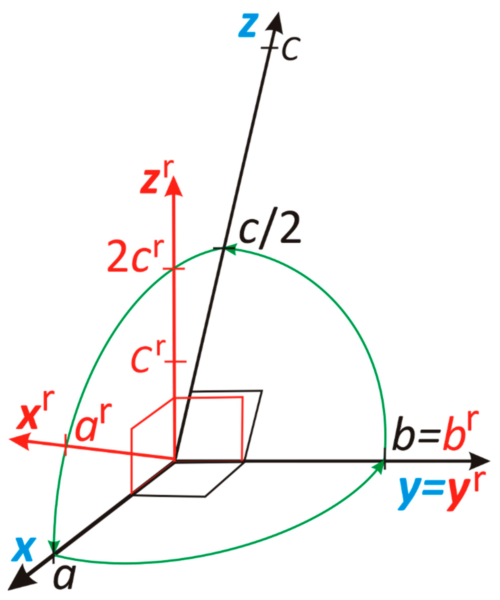
Figure 2.
A hexagonal lattice projected along [z], with hexagonal coordinates of nodes along directions[x], [y] and at z = 0.
Figure 2.
A hexagonal lattice projected along [z], with hexagonal coordinates of nodes along directions[x], [y] and at z = 0.
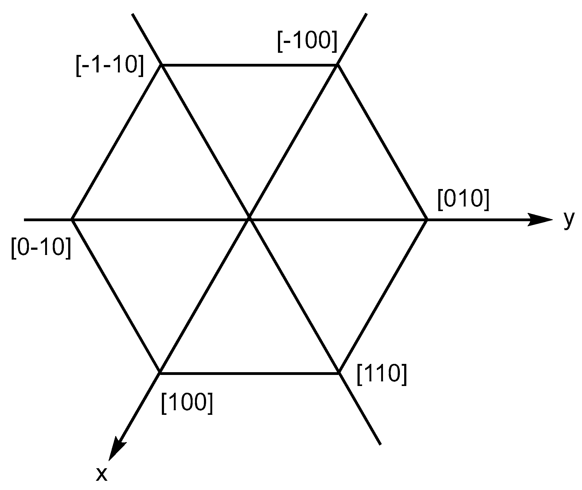
Table 1.
Symmetry elements for the trigonal system and their quaternion representations for the hexagonal reference axes (cf. Table 6 in Reference [21]).
| Symmetry element | Quaternion (q) | Quaternion action |
|---|---|---|
| 1 | 1 | qr |
| 1 | qr | |
| 2[100] | i | qrq* |
| 2[010] | j | qrq* |
| 2[110] | i+j | qrq* |
| 3[001] | qrq* | |
| –qrq* | ||
| m[100] | i | qrq |
| m[010] | j | qrq |
| m[110] | i+j | qrq |
Table 2.
Symmetry elements for the hexagonal system and the quaternion representations of symmetry operations in the crystal reference setting (cf. Table 1).
Table 2.
Symmetry elements for the hexagonal system and the quaternion representations of symmetry operations in the crystal reference setting (cf. Table 1).
| Symmetry operation | Quaternion (q) | Quaternion action |
|---|---|---|
| 1 | 1 | qr |
| 1 | qr | |
| qrq* | ||
| qrq* | ||
| qrq* | ||
| qrq* | ||
| qrq* | ||
| qrq* | ||
| qrq* | ||
| qrq* | ||
| qrq* | ||
| qrq* | ||
| qrq | ||
| qrq | ||
| qrq | ||
| qrq | ||
| qrq |
Table 3.
Multiplication table for biquaternions (Equation 13) in the representation of symmetry operations of the point group (Ci).
Table 3.
Multiplication table for biquaternions (Equation 13) in the representation of symmetry operations of the point group (Ci).
| 1 | h | |
| h | –1 |
Table 4.
Multiplication table of biquaternions (Equation 13) used in representing the symmetry operations in point group mm2 (C2v).
Table 4.
Multiplication table of biquaternions (Equation 13) used in representing the symmetry operations in point group mm2 (C2v).
| mm2 | 1 | 2 | mx | my |
| 1 | 1 | k | hi | hj |
| 2 | k | –1 | –hj | hi |
| mx | hi | hj | 1 | k |
| my | hj | –hi | –k | 1 |
Table 5.
Multiplication Cayley table of the symmetry operations in point group mm2 (C2v).
| mm2 | 1 | 2 | mx | my |
| 1 | 1 | 2 | mx | my |
| 2 | 2 | 1 | my | mx |
| mx | mx | my | 1 | 2 |
| my | my | mx | 2 | 1 |
Disclaimer/Publisher’s Note: The statements, opinions and data contained in all publications are solely those of the individual author(s) and contributor(s) and not of MDPI and/or the editor(s). MDPI and/or the editor(s) disclaim responsibility for any injury to people or property resulting from any ideas, methods, instructions or products referred to in the content. |
© 2024 by the authors. Licensee MDPI, Basel, Switzerland. This article is an open access article distributed under the terms and conditions of the Creative Commons Attribution (CC BY) license (http://creativecommons.org/licenses/by/4.0/).
Copyright: This open access article is published under a Creative Commons CC BY 4.0 license, which permit the free download, distribution, and reuse, provided that the author and preprint are cited in any reuse.


