Submitted:
04 September 2024
Posted:
04 September 2024
You are already at the latest version
Abstract
This paper examines the determinants of CO2 emissions in Oman from 1990 to 2022, focusing on the impacts of energy consumption, economic growth, urbanization, financial development, and foreign direct investment. Utilizing stepwise regression, robust least squares, Fully Modified Least Squares (FMOLS), Canonical Cointegrating Regression (CCR), and various cointegration tests including the Johansen cointegration test, Engle-Granger cointegration test, and Vector Error Correction (VEC) model, the study reveals several key findings. Energy use per capita (ENGY) and real GDP per capita (RGDPC) are consistently significant positive predictors of CO2 emissions. Urbanization (URB) also significantly contributes to higher emissions. Conversely, Financial Development Index (FDX) and foreign direct investment (FDI) do not show significant effects on CO2 levels. The high R-squared values across models indicate that these variables explain a substantial portion of the variation in emissions. Cointegration tests confirm long-term equilibrium relationships among the variables, with the Johansen test identifying two cointegrating equations and the Engle-Granger test showing significant tau-statistics for FDX, ENGY, and URB. The VEC model further highlights the short-term dynamics and adjustment mechanisms. These findings underscore the importance of energy policy, economic development, and urban planning in Oman's efforts towards sustainable development and decarbonization.
Keywords:
Decarbonization
; Energy Transition
; Oman
; Cointegration
1. Introduction
Oman, strategically located on the southeastern coast of the Arabian Peninsula, has experienced dramatic transformation over the past four decades, largely fueled by its oil and gas industry. This sector has not only driven economic growth and increased export revenue but also spurred extensive infrastructure and industrial development, shaping Oman into a modernized nation with elevated living standards. As described by researchers like [1,2], the oil and gas industry has been integral to Oman’s contemporary renaissance, making it difficult to imagine the country’s economy without it.
Despite these advancements, Oman now stands at a critical juncture. The global push towards sustainability and reduced carbon emissions presents a significant challenge, requiring a strategic decarbonization of its economic systems. This transition aims to preserve the high standard of living for its populace while minimizing adverse impacts on the social, economic, and political fabric of the country, as discussed by [3,4,5].
This paper delves into Oman’s efforts to navigate this complex transition. It examines the interplay between economic growth, governance, and sustainable practices within the context of Oman's unique geopolitical and socio-economic landscape. Through a comprehensive analysis using data from 1990 to 2022, this study employs econometric techniques to explore the long-term relationships between CO2 emissions, economic variables, and governance indicators. The findings not only highlight the significant variability and challenges in CO2 emissions but also demonstrate the critical long-term relationships essential for formulating effective policies. By exploring Oman’s ongoing commitment to energy diversification and technological innovation, this paper illuminates the pathways that could lead Oman towards a more sustainable and resilient future.
1.1. Background
Understanding the background is crucial for appreciating the significance of decarbonization and the energy transition process in the context of contemporary climate change challenges. Historically, hydrocarbons have been the cornerstone of the Omani economy, serving as its primary energy source and driving economic activities across various sectors. Research indicates that approximately 30% of Oman's primary energy supply is allocated to power generation, with the remaining portion distributed among industrial, residential, transportation, and commercial sectors [6]. This highlights the critical role of natural gas in Oman's energy landscape, underpinning its energy-intensive economy bolstered by the government's reinvestment of petroleum profits. However, this focus has resulted in minimal emphasis on energy efficiency [7].
Energy efficiency is crucial for extending the lifecycle of finite energy resources while maintaining quality of life. It involves using less energy to achieve the same output, which can significantly reduce operational costs and environmental impacts across various sectors, including residential, industrial, and energy-intensive industries like oil and gas [8]. The current approach in Oman, characterized by insufficient focus on energy efficiency, exacerbates the rate of hydrocarbon depletion, potentially accelerating the depletion of these essential resources. Such a scenario not only risks escalating energy prices across all sectors but also positions Oman on a precarious path towards becoming energy-dependent. If unaddressed, this could transition Oman from an energy-exporting to an energy-importing country, thereby straining the national economy which has been historically buoyed by energy exports [9,10,11].
In the long term, recognizing the interconnectedness of these factors—excessive hydrocarbon usage, low energy efficiency, environmental oversight, and rising energy costs—is essential for strategic planning. It necessitates a shift towards renewable energy resources, thereby aligning Oman's economic and environmental policies with global sustainability targets. This transition is critical not only for reducing the environmental footprint but also for ensuring economic stability and energy security in Oman.
1.2. Objectives and Motivation
The primary objective of this study, is to analyze the determinants of CO2 emissions in Oman from 1990 to 2022, focusing on the roles of energy consumption, economic growth, urbanization, domestic credit, and foreign direct investment. By employing advanced econometric techniques, including stepwise regression, robust least squares, Fully Modified Least Squares (FMOLS), Canonical Cointegrating Regression (CCR), and multiple cointegration tests, the study aims to provide a comprehensive understanding of the factors driving CO2 emissions in Oman. The motivation behind this research is to inform policy-makers about the critical areas requiring intervention to achieve sustainable development and decarbonization. Given Oman's commitment to the Paris Agreement and its national objectives for reducing carbon footprints, this study seeks to highlight the interplay between economic activities and environmental impacts. It underscores the necessity of developing energy policies, urban planning, and economic strategies that align with sustainability goals, ultimately contributing to Oman's green transition and long-term environmental resilience.
1.3. Research Problem
Oman's commitment to attaining net zero greenhouse gas emissions by 2050 represents a significant and complex challenge in light of its existing energy infrastructure. This ambitious target necessitates a profound transformation of the energy sector to achieve carbon neutrality. Thus, it is crucial to develop a comprehensive understanding of the potential pathways for transitioning to a sustainable energy system. The research problem centers on identifying and evaluating these optimal transition pathways, considering the economic implications and the necessary policy frameworks that could support this shift. It is imperative to analyze how various factors—such as economic growth, foreign direct investment, energy consumption, and urbanization—interact and influence the decarbonization process. This study will employ econometric techniques to explore these dynamics using panel data from 1990 to 2022, aiming to provide actionable insights that could guide policy formulation and sustainable development strategies in Oman.
2. Energy Transition and Decarbonization Initiatives in Oman
2.1. key developments and initiatives in Oman related to energy transition and decarbonization
Oman is making significant strides in its decarbonization and energy transition efforts, particularly through investments in renewable energy sources like solar and wind. The Miraah solar plant, with a capacity of 7 GW, is pivotal in producing green hydrogen, generating approximately 9.78 TWh annually, which aligns with Oman Vision 2040's sustainability goals [12]. Additionally, the Dhofar Wind Power Project contributes to this renewable energy landscape, enhancing the country's capacity to reduce greenhouse gas emissions [13].
Oman is classified among the top countries that enjoys high solar irradiation 7340.19 Wh/m2/day (See Figure 1). Also, Oman has tremendous amounts of wind recourses specially in the southern part. Wind has no pattern in variation during the year. Cut in/ cut out feature of wind turbines impacted the generation, (See Figure 2).
Improving energy efficiency remains a core component of Oman's strategy, with government policies encouraging sustainable practices across industries, transportation, and residential sectors to cut energy use and emissions. Additionally, Oman is exploring carbon capture and storage (CCS) technologies, led by the Oman Carbon Capture Company, which could significantly mitigate industrial emissions. The nation is also tapping into its geographical advantages and renewable resources to explore hydrogen production, conducting pilot projects to evaluate the feasibility of this alternative energy source for potential future export. Moreover, Oman is enhancing its sustainable transportation infrastructure, investing in electric vehicle charging stations and public transportation systems to curb emissions from its expanding transportation sector [14].
2.2. National Strategies and Policies
The Sultanate of Oman has embarked on a strategic pathway to a sustainable and economically prosperous future through a comprehensive decarbonization and energy transition strategy. Key national policies and strategic directives reflect a governmental vision focused on limiting future reliance on conventional resources and promoting sustainable development to ensure security and prosperity for future generations. The government is aiming for a renewable energy share of 10% by 2025, escalating to 30% by 2030, and reaching 50% by 2040. These targets are designed not only to reduce carbon emissions but also to drive economic growth through job creation, training, and research in the renewable energy sector [12].
Oman's Ministry of Energy and Minerals (MEMR) has outlined initiatives such as achieving up to 8% savings on natural gas and oil used in power generation, and setting an investment target of 22 billion in renewable energy by 2025 in collaboration with the private sector. These investments aim to stimulate energy transformation projects, fostering employment for skilled professionals, and ensuring energy reliability for the future. [16].
In addition, the Public Authority for Electricity and Water (PAEW) has implemented a 10% renewable purchase obligation, aiming to reduce energy intensity by 30% and gas utilization from 70% to 25% by 2040. This ambitious transition from a gas-based economy to a low carbon energy mix is critical but challenging, especially with the potential economic impacts of sustained low oil and gas prices. The regulatory framework needs to provide clear guidance and stability to encourage significant capital investments in renewable projects to meet these future energy mix quotas without imposing additional costs on consumers.
In the realm of renewable energy development, Oman has prioritized investments in solar energy technologies, including several initiatives for rural electrification and water pumping systems powered by photovoltaics (PV). A noteworthy project is the collaboration between the Ministry of Oil and Gas (MOG) and PDO to implement a 50MW solar-generated thermal enhanced oil recovery system in the Amal field, which is expected to reduce gas consumption and provide hands-on experience in Solar EOR techniques [17]. Chart 1 provides summary of these initiatives.
Overall, Oman's strategic approach to sustainability through decarbonization and energy transition is robust, aligning with global trends and regional imperatives to foster economic diversification and long-term environmental stewardship.
3. Literature Review
Oman is making efforts to achieve a sustainable future by navigating decarbonization and energy transition. The utilization of hybrid power systems, such as PV-wind-diesel systems, is being explored to reduce diesel fuel consumption and greenhouse gas emissions in rural areas [18]. The management of water and wastewater is also being addressed, with a focus on progressive reuse applications and the production of green hydrogen from treated effluent, [19]. Oman has set a target of achieving net zero emissions by 2050 and is implementing environmental measures to reach this goal [20]. The country's efforts align with global climate objectives and the transition to cleaner economies [21].
Oman's transition to a sustainable future and decarbonization is a topic explored in several empirical literature. The adverse impact of energy production from fossil fuels is recognized globally, and Oman aims to achieve the UN Sustainable Development Goals by adopting renewable and sustainable energy sources [22]. However, the political-economic structures of oil-producing Gulf Arab states, including Oman, have hindered the adoption of renewable energy, with a focus on protecting rents from oil exports rather than advancing low-carbon energy transition [23]. Oman has significant potential for wind energy, particularly in the Governorate of Dhofar, where wind farms are being developed to increase the country's wind energy output [24]. Waste management strategies in Oman, including waste-to-energy technologies, are also being explored to address environmental sustainability and increase power grid capability [25] These empirical studies provide insights into Oman's efforts to navigate decarbonization and energy transition towards a sustainable future.
The empirical literature on MENA's path to a sustainable future, navigating decarbonization and energy transition, highlights several key factors. High oil and gas prices have incentivized MENA hydrocarbon importers and exporters to accelerate their renewables build-outs, driven by global decarbonization targets and climatic advantages. Psychosocial research on sustainability emphasizes the importance of understanding psychosocial processes at different levels, including the individual, community, and socio-cultural levels, but also identifies biases and research gaps [26]. The MENA region faces challenges in retooling domestic hydrocarbon industries, introducing renewables, and diversifying economies, amidst falling resource rents and geopolitical shifts Robin, [27]. Energy transitions require a fundamental change in social relations and can be governed through inclusive multistakeholder dialogues [28]. Transition research analyzes concepts and roadmaps for transforming MENA's energy systems, identifying key drivers, barriers, and indicators for monitoring sustainability [29].
The empirical literature on the Gulf Cooperation Council (GCC) countries' path to a sustainable future, focusing on decarbonization and energy transition, highlights several key findings. Firstly, there is a serious need for the GCC countries to address the rising threat of climate change and its impact on the region's economy and environment [21] Secondly, the association between CO2 emissions and factors such as electricity consumption, economic growth, urbanization, and trade openness has been investigated using the wavelet coherence approach, providing valuable policy recommendations for environmental planning and sustainable energies in the Gulf region [30]. Thirdly, the geopolitical implications of the global energy transition towards low-carbon renewable energy sources in the Arab Gulf states have been examined, revealing inconsistencies and disagreements among studies and emphasizing the need for multi coherent frameworks to understand the nature of the geopolitical impact [31]. Lastly, the role of renewable energy sources in the GCC countries' energy policy, along with factors limiting their development, has been analyzed, highlighting the prospects for further energy policy development in the region [32].
4. Model, Data, and Econometric Strategy
4.1. Model
The objective of this study is to investigate the dynamic relationship between decarbonization, economic growth, and other relevant factors in Oman. The following model which is similar [33, 34], .to is used to examine this interconnected relationship:
Ln CO2 = α0 + α1Ln RGDPCit + α2Ln ENGYit + α3 Ln URBit +α4 FDIit+ α5 FDX it + εit
In the given model, you have specified a multiple regression equation with Ln CO2 (natural logarithm of carbon dioxide emissions) as the dependent variable. Let's delve into the independent variables and discuss their likely effects on Ln CO2, whether they are positive or negative, (See Section 3.2 and Table 1)
4.2. Data, Variable Description & Expected Sign of Parameters
- Ln RGDPCit (Per Capita GDP): The coefficient α1 represents the effect of per capita GDP on carbon emissions. Typically, as a country's per capita GDP increases, it indicates higher economic development. In this context, a positive relationship is often observed, meaning that as the economy grows, carbon emissions tend to increase due to increased industrialization, energy consumption, and transportation. Therefore, α1 is likely to be positive, α1 > 0
- ENGYit (Energy Use): The coefficient α2 represents the effect of energy use per capita on carbon emissions. Higher energy use is generally associated with higher carbon emissions, as most energy sources involve the combustion of fossil fuels. Hence, α2 is also likely to be positive. α2 > 0
- URBit (Urban Population Percentage): The coefficient α3 signifies the impact of the percentage of urban population on carbon emissions. Urbanization often leads to increased energy consumption and emissions due to factors like increased transportation and energy demand. Thus, α3 is likely to be positive. α3 > 0.
- FDIit (Foreign Direct Investment): The relationship between FDI and emissions can vary. FDI may lead to technology transfer and increased efficiency, potentially reducing emissions (negative effect). However, it can also drive industrialization and increased production, leading to higher emissions (positive effect). The actual direction of α4 will depend on the specific context, (α4 < 0 or α4 > 0)
- FDX it (Financial Development Index): A developed financial sector can promote green investments and sustainable practices, potentially reducing emissions (negative effect). Conversely, if financial development leads to increased industrial activity, it might raise emissions (positive effect). Like other variables, the direction of α6 will depend on specific circumstances. (α5 < 0 or α5 > 0)
- εit (Error Term): The error term εit captures unexplained variation in carbon emissions that is not accounted for by the independent variables in the model. It encompasses other factors and random variability.
3.2. Econometric Methodology
The core econometric methodologies at our disposal include the Fully Modified Least Squares (FMOLS), Stepwise Regression, Robust Least Squares, ML - ARCH (Marquardt) - Normal distribution, estimation method, the Johansen cointegration test, and the error correction model (ECM), Canonical Cointegrating Regression (CCR), Cointegration Test - Hansen Parameter Instability, Cointegration Test - Engle-Granger. These methodologies are well-suited for examining the long-term relationships, short-term dynamics, and causal linkages between CO2 and other variable in Oman.
3.2.1. Johansen cointegration test
For investigating potential cointegration among the variables in the model, we can employ the Johansen cointegration test, which is appropriate for multivariate time series analysis. The Johansen test allows us to determine the presence and rank of cointegration among the variables.
The cointegration model can be specified as follows:
ΔY = ΠYt−1+Γ1ΔYt−1+Γ2ΔYt−2+...+Γp−1ΔYt−(p−1) +ϵt
Where:
- Yt is a vector of the variables included in the model (e.g., CO2 emissions, per capita GDP, energy use per capita, etc.).
- Π is a matrix of cointegration parameters.
- Γi are coefficient matrices for the first differences of the variables up to lag p.
- ϵt is the error term.
3.2.2. Canonical Cointegrating Regression (CCR)
Canonical Cointegrating Regression (CCR) is a method used to estimate the long-run relationship between non-stationary time series variables that are cointegrated. This method, proposed by Peter C.B. Phillips, modifies the ordinary least squares (OLS) approach to account for the endogeneity and serial correlation that typically arise in cointegrated systems. By transforming the data, CCR produces consistent estimates of the cointegrating vectors.
Consider a set of time series variables Yt and Xt that are integrated of order one, I (1), and cointegrated. The canonical cointegrating regression can be specified as:
where:
Yt=β0+β1X1t+β2X2t+...+βkXkt+ϵt
- Yt is the dependent variable at time t.
- X1t, X2t,…,Xkt are the independent (cointegrating) variables at time t.
- β0 is the intercept term.
- β1,β2,…,βk are the cointegrating coefficients to be estimated.
- ϵt is the error term at time t, which is assumed to be stationary.
3.2.3. The error correction model (ECM)
The error correction model (ECM) is a framework used to analyze the short-term and long-term interactions between variables in a cointegrated relationship. The standard ECM equation takes the following form
The ECM can be specified as follows:
ΔYt=α(Yt−1−Βxt−1) +Γ1ΔYt−1+Γ2ΔYt−2+…+Γp−1ΔYt−(p−1) +ϵt
Where:
- Xt−1 represents the lagged values of the cointegrating variables.
- α is the coefficient of the error correction term, representing the speed of adjustment towards the long-run equilibrium.
- β is the coefficient matrix of the cointegrating vector(s).
- The remaining terms are as defined in the previous model.
Estimating the ECM allows us to examine both short-term dynamics and long-term equilibrium relationships among the variables in the model, providing valuable insights into the sustainability and economic development dynamics in Oman.
3.2.4. Stepwise Regression
Stepwise regression is a method of fitting regression models in which the choice of predictive variables is carried out by an automatic procedure. This process involves iteratively adding or removing predictors based on specific criteria, usually the Akaike Information Criterion (AIC), Bayesian Information Criterion (BIC), or p-values of the estimated coefficients. The goal is to find the most parsimonious model that explains the data well. The following is an example of an econometric equation:
Assume we have three potential predictors X1, X2, and X3.. The stepwise regression might proceed as follows:
- Start with no variables: Y=β0+ϵ
- Add the most significant variable (e.g., X1): Y=β0+β1X1+ϵ
- Evaluate and possibly add X2: Y=β0+β1X1+β2X2+ϵ
-
Check if X1 or X2 become insignificant and remove if necessary:
- ○
- If both are significant, keep both.
- ○
- If X1 becomes insignificant after adding X2: Y=β0+β2X2+ϵ
- Continue by evaluating X3: Y=β0+β1X1+β2X2+β3X3+ϵ
The final econometric model after stepwise regression might look like:
Y=β0 + β1X1 + β3X3 + ϵ
This represents a model where only X1 and X3 are retained as significant predictors of Y after the stepwise selection process.
3.2.5. Fully Modified Least Squares (FMOLS)
Fully Modified Least Squares (FMOLS) is an econometric technique used to estimate a regression model where the variables may be endogenous and exhibit potential serial correlation. It is particularly useful in addressing issues related to non-stationarity in time series data. The FMOLS regression equation generally takes the following form:
where:
Yt=β0+β1X1t+β2X2t+…+βkXkt+ϵt
- Yt is the dependent variable at time t.
- X1t, X2t,…,Xkt_ are the independent variables at time t.
- β0,β1,β2,…,βk are the coefficients to be estimated.
- ϵt is the error term assumed to be white noise,
In the context of FMOLS, additional adjustments are made to address potential endogeneity and non-stationarity in the variables. The estimator is designed to be robust to these issues, often involving the use of instrumental variables and correcting for the presence of unit roots (non-stationarity).
5. Results
5.1. Descriptive Statistics
Based on the summary statistics provided for the series CO2, FDX, ENGY, FDI, RGDPC, and URB, several observations can be made. The data suggests variability across the variables: CO2 emissions (mean = 12.58, SD = 3.58) show moderate spread with slight negative skewness and mild kurtosis, indicating a generally normal distribution. FDX (mean = 41.99, SD = 16.26) and ENGY (mean = 4691.03, SD = 1597.08) exhibit higher variability, with ENGY skewed slightly left and FDI (mean = 2.00, SD = 2.17) showing positive skewness. RGDPC (mean = 18599.18, SD = 1913.77) and URB (mean = 75.65, SD = 6.03) display relatively lower variation, with URB showing positive skewness.
The coefficients of variation (C.V) provide a standardized measure of dispersion relative to the mean for each variable. Higher values indicate greater relative variability, highlighting FDX as the most variable among the listed variables, followed by ENGY and CO2.
Following the descriptive analysis, Figure 3 illustrates the factors influencing CO2 variations over time. The graph provides a comprehensive view of CO2 levels over time, depicting both the concerning long-term rise in CO2 levels, likely attributed to human activities such as fossil fuel combustion, and the natural seasonal fluctuations stemming from biological and ecological processes.
5.2. Stepwise Regression
The regression results presented in Table 3 reveal several significant findings. Energy use (ENGY) has a positive and statistically significant coefficient (0.001207, t = 4.027), indicating that increased per capita energy consumption is associated with higher CO2 emissions, this result is similar to the result obtained by [36]. Real GDP per capita (RGDPC) also shows a positive and significant coefficient (0.000676, t = 4.266), suggesting that economic growth contributes to increased CO2 levels. Urbanization (URB) displays a positive coefficient (0.344981, t = 2.544), significant at the 5% level, implying that urban development impacts CO2 emissions. In contrast, domestic credit provided by the financial sector (FDX), and foreign direct investment (FDI), do not exhibit statistically significant relationships with CO2 levels, as indicated by their respective coefficients and t-statistics. The high R-squared value (0.923) suggests that the model explains a substantial portion of the variation in CO2 emissions, highlighting the robustness of the identified relationships.
5.3. Robust Check
The results from Table 4 using the Robust Least Squares method provide valuable insights into the factors influencing CO2 emissions. The model shows that ENGY (energy consumption) and RGDPC (real GDP per capita) are statistically significant predictors of CO2 emissions, with positive coefficients of 0.001320 and 0.000630, respectively, indicating that increases in energy consumption and GDP per capita lead to higher CO2 emissions. URB (urbanization) also has a positive and significant impact with a coefficient of 0.331275, suggesting that higher urbanization levels contribute to increased CO2 emissions. The variable FDX (Development Policy) and FDI (Foreign Direct Investment), however, show non-significant coefficients, implying they do not have a substantial effect on CO2 emissions in this model. The intercept (C) is significantly negative, indicating a baseline reduction in CO2 emissions when other factors are controlled. The model's R-squared and adjusted R-squared values (0.704947 and 0.650307, respectively) suggest a good fit, explaining around 65-70% of the variation in CO2 emissions. The robust R-squared (0.950575) indicates a high level of explanatory power when accounting for potential outliers and heteroscedasticity. Overall, the Robust Least Squares results highlight the critical roles of energy consumption, GDP per capita, and urbanization in driving CO2 emissions, underscoring the importance of these factors in environmental policy and sustainable development strategies.
5.4. Unit Root Test
Table 5 summarizes the results of the Augmented Dickey-Fuller (ADF) tests, illustrating the transformation of non-stationary variables into stationary ones through first differencing. Initially, all variables—CO2 emissions, real GDP per capita (RGDPC), energy consumption (ENGY), foreign direct investment (FDI), domestic credit provided by the financial sector (FDX), urban population (URB)—displayed non-stationary behavior in their original forms (I (0)), as evidenced by ADF test statistics above critical values and p-values exceeding 0.05. However, after applying first differencing, all variables exhibited significant improvements, with ADF test statistics falling below critical values and p-values decreasing substantially (all ≤ 0.01), confirming their transformation to stationarity (I(1)). This transformation is crucial for ensuring the reliability of time series analyses and forecasting models, underscoring the importance of preprocessing techniques in enhancing the accuracy and robustness of economic and financial research.
5.5. The Johansen cointegration test
The Johansen cointegration test results (Table 6), indicate significant long-term relationships among the variables CO2, FDX, ENGY, FDI, RGDPC, and URB. The test shows that there are two cointegrating equations at the 5% significance level, as evidenced by the rejection of the null hypothesis for models with up to 4 lags in first differences. This suggests that despite their individual short-term dynamics, these variables are linked by stable, long-run relationships that move together over time. The low p-values (Prob.**) associated with the trace statistics further support the rejection of the null hypothesis, confirming the existence of these cointegrating relationships. These findings are crucial for understanding how these economic and environmental factors interact and jointly influence CO2 emissions, providing a basis for modeling and policy analysis aimed at sustainable development and climate mitigation strategies.
5.6. The Canonical Cointegrating Regression (CCR)
The Canonical Cointegrating Regression (CCR) results (Table 7) indicate significant long-term relationships between CO2 emissions and the variables FDX, FDI, ENGY, RGDPC, and URB. Energy use per capita (ENGY) and real GDP per capita (RGDPC) show positive and statistically significant coefficients (ENGY: 0.001324, t = 4.431; RGDPC: 0.000698, t = 4.466), suggesting that higher energy consumption and economic output per capita are associated with increased CO2 emissions. Urbanization (URB) also exhibits a positive and significant coefficient (0.286755, t = 2.129) at the 5% level, indicating that urban development influences CO2 levels. Conversely, financial development index (FDX)) and foreign direct investment (FDI) do not show statistically significant relationships with CO2 emissions based on their respective coefficients and t-statistics. The model's high adjusted R-squared (0.896) indicates that a substantial portion of the variation in CO2 emissions is explained by the included variables, reinforcing the robustness of these long-run relationships. The findings underscore the importance of energy policy, economic development strategies, and urban planning in addressing and mitigating CO2 emissions in the context of sustainable development goals.
5.7. the Engle-Granger cointegration test
Based on the Engle-Granger cointegration test results (Table 8), FDX (Financial Sector Development Index), ENGY (Energy Use per capita), and URB (Urbanization Rate) exhibit tau-statistics with p-values below conventional significance levels, suggesting strong evidence against the null hypothesis that these variables are not cointegrated with CO2 emissions. Specifically, FDX, ENGY, and URB show tau-statistics of -4.102383, -3.970701, and -4.408060, respectively, with corresponding p-values of 0.2905, 0.3369, and 0.1949. These findings indicate that changes in FDX, ENGY, and URB are associated with long-term changes in CO2 emissions, highlighting their interconnectedness and potential roles in influencing environmental outcomes.
5.8. The Vector Error Correction (VEC)
The Vector Error Correction Estimates in Table 9 provide insights into the short-term dynamics and equilibrium relationships among the variables. The coefficients from the cointegrating equation CointEq1 indicate that FDX(-1), ENGY(-1), URB(-1), RGDPC(-1), and FDI(-1) have significant impacts on CO2 emissions over time. Notably, URB(-1) stands out with a coefficient of -5.785633 (t-statistic = -14.5139), suggesting a strong negative relationship between previous period urbanization rates and current CO2 emissions. This indicates that changes in urbanization levels exert a substantial short-term correction effect on CO2 emissions, highlighting the critical role of urban development policies in environmental sustainability efforts. The Error Correction terms further detail the adjustments towards equilibrium, underscoring the importance of these variables in modeling and forecasting CO2 emissions dynamics.
5.9. Fully Modified Least Squares (FMOLS)
The results from the Fully Modified Least Squares (FMOLS) estimation in Table 10 reveal several key insights into the relationship between CO2 emissions (the dependent variable) and various independent variables. The model indicates a high degree of explanatory power with an adjusted R-squared of 0.8996, suggesting that approximately 90% of the variation in CO2 emissions can be explained by the included variables.
Variables such as ENGY (related to energy), RGDPC (real GDP per capita), and URB (urbanization) show statistically significant coefficients with t-statistics indicating robustness. Specifically, ENGY and RGDPC exhibit positive coefficients (0.001340 and 0.000657, respectively), implying that increases in energy consumption and GDP per capita lead to higher CO2 emissions. On the other hand, the coefficient for URB is positive but marginally statistically significant (p = 0.0506), suggesting that urbanization also plays a role, albeit less decisively. The intercept (C) is negative and statistically significant, indicating a base level of CO2 emissions that decreases as other factors are controlled. However, variables like FDX (Development Policy) and FDI (Foreign Direct Investment) show coefficients that are not statistically significant, suggesting that their impact on CO2 emissions in this model is less clear. Overall, the FMOLS results provide a detailed understanding of how economic and demographic factors influence CO2 emissions over the long term, underscoring the complexity of sustainable development challenges.
6. Diagnostic Tests
The diagnostic results presented in Table 11 indicate that the model is robust and reliable. The Jarque-Bera test demonstrates that the residuals follow a normal distribution, which is crucial for the validity of standard statistical tests. The Breusch-Godfrey LM analysis reveals no evidence of serial correlation, suggesting that the error terms are independent. Likewise, the Breusch-Pagan-Godfrey test shows no heteroscedasticity, indicating that the variance of the errors is consistent across observations. The stability test confirms the model's stability over time, with no structural breaks. Furthermore, the Ramsey RESET analysis indicates that the model is correctly specified, with no significant evidence of omitted variable bias or incorrect functional form. Overall, the diagnostics affirm that the model is well-specified and reliable.
Furthermore, to verify model stability, the study employed the CUSUM and CUSUMSQ tests. These tests assess the stability of the model, and the corresponding charts at a 5% significance level are illustrated in Figure 4. In the charts, the residuals are outlined in blue, while the confidence intervals are represented by red lines. At the 5% significance level, it is evident that the residuals of the variables consistently remain within the confidence intervals, indicating that the model is stable
Figure 5 illustrates the inverse of the Autoregressive (AR) characteristic polynomial, which is fundamental in time series analysis for describing how past values influence the current value of a series. The inverse polynomial reveals the roots of the AR model and their implications for its behavior and stability. In Figure 5, if all inverse roots are within the unit circle, as observed, it indicates that the time series model is stable. This stability is crucial as it ensures the model can reliably generate consistent forecasts over time. Given our findings, where this stability criterion is satisfied, we can confidently proceed with using the model for forecasting and further analysis.
7. Discussion
The results of this study strongly demonstrate a significant connection between energy consumption, economic growth, and CO2 emissions in Oman, echoing findings from previous research on the environmental impacts of these factors. The analysis reveals that both energy consumption per capita and real GDP per capita are positively linked to CO2 emissions, which aligns with the environmental Kuznets curve (EKC) hypothesis. This theory suggests that environmental degradation increases during the early stages of economic growth but begins to decline once a certain income level is reached, as more resources are dedicated to environmental protection and the adoption of cleaner technologies [38, 39]). Such a pattern has been observed in various developing economies, especially those experiencing rapid industrialization and urbanization, similar to Oman [40]. The significant association between energy consumption, GDP, and CO2 emissions highlighted in this study underscores the urgent need for Oman to adopt cleaner energy technologies and enhance energy efficiency to reduce the environmental impact of its economic growth.
The study also emphasizes the critical role of urbanization as a key driver of CO2 emissions, a finding that is consistent with other research focusing on rapidly developing regions. As urban areas in Oman expand, the demand for energy in residential, industrial, and transportation sectors increases, leading to higher CO2 emissions [41]. This trend is particularly concerning given the fast pace of urban expansion, which puts additional pressure on the environment. The positive correlation between urbanization and emissions highlights the importance of incorporating sustainable urban planning practices into Oman’s development strategy. Steps like advancing energy-efficient building practices, enhancing public transportation systems, and boosting investments in renewable energy are crucial for tackling the environmental issues brought on by urbanization. By implementing these strategies, Oman can reduce the carbon footprint of its urban development and ensure its growth aligns with global sustainability goals.
Furthermore, the study reveals the complexity of the relationship between financial development, foreign direct investment (FDI), and CO2 emissions. While the results indicate that financial development and FDI do not have a significant direct impact on CO2 emissions in Oman, this does not mean these factors are unimportant for environmental outcomes. The environmental effects of financial development and FDI are often influenced by other factors such as the type of investments, the regulatory framework, and the overall economic structure [42]. For instance, FDI can either increase or decrease CO2 emissions depending on whether the investments are channeled into environmentally friendly projects or energy-intensive industries. Therefore, while financial development and FDI may not directly affect emissions, they have the potential to significantly contribute to a low-carbon economy if they are aligned with sustainable development objectives.
Finally, the policy implications of this study are particularly pertinent for Oman’s efforts to balance its environmental and economic goals. Policymakers should prioritize establishing a regulatory environment that encourages green investments and motivates the financial sector to support sustainable development initiatives. This could include offering tax incentives or subsidies for investments in renewable energy, energy-efficient technologies, and sustainable urban infrastructure. Additionally, Oman’s financial sector should be encouraged to create green financing products that facilitate the transition to a low-carbon economy. By leveraging financial development and FDI to promote sustainable practices, Oman can drive economic growth while minimizing environmental degradation [40]. Such a comprehensive approach is essential to ensure that Oman’s economic development is environmentally sustainable and resilient in the face of global environmental challenges.
8. Conclusion
This study provides a comprehensive analysis of the determinants of CO2 emissions in Oman over the period from 1990 to 2022, focusing on the roles of energy consumption, economic growth, urbanization, and foreign direct investment. By employing a range of econometric techniques including stepwise regression, robust least squares, Fully Modified Least Squares (FMOLS), Canonical Cointegrating Regression (CCR), Johansen cointegration test, Engle-Granger cointegration test, and Vector Error Correction (VEC) model, we have gained robust insights into the long-term and short-term dynamics influencing CO2 emissions in Oman.
The empirical findings consistently indicate that energy use per capita (ENGY) and real GDP per capita (RGDPC) are significant positive predictors of CO2 emissions. This underscores the critical role of energy consumption and economic growth in driving emissions, suggesting that increases in these areas lead to higher levels of CO2. Urbanization (URB) also emerges as a significant factor, contributing to higher emissions as urban areas expand and develop. Conversely, financial development index (FDX) and foreign direct investment (FDI) do not show significant impacts on CO2 emissions in most models, indicating that their roles in environmental outcomes may be more complex and indirect.
The high R-squared values across the different models, along with the robust cointegration relationships identified, confirm the reliability and stability of these findings. The Johansen cointegration test reveals two significant long-term equilibrium relationships among the variables, while the Engle-Granger test highlights the significance of FDX, ENGY, and URB in the long-term dynamics of CO2 emissions. The VEC model further elucidates the short-term adjustments and the pathways through which these variables influence emissions over time.
Policy Implications: The insights derived from this study have significant policy implications for Oman's efforts to achieve sustainable development and decarbonization. Given the positive relationship between energy consumption and CO2 emissions, it is imperative for policymakers to prioritize energy efficiency and promote the adoption of renewable energy sources. Economic growth strategies should be designed to balance development with environmental sustainability, ensuring that increases in GDP do not lead to proportional rises in emissions. Urban planning must incorporate sustainable practices, focusing on reducing the carbon footprint of cities through green infrastructure, efficient public transport systems, and smart city initiatives.
While financial development and foreign direct investment do not show direct impacts on emissions, financial policies should still encourage investments in green technologies and sustainable business practices. This includes providing incentives for businesses and industries to reduce their carbon footprint and supporting research and development in clean energy technologies.
In conclusion, a holistic and integrated policy framework that addresses the key drivers of CO2 emissions—energy use, economic growth, and urbanization—is essential for Oman to transition towards a sustainable and low-carbon economy. By leveraging these insights, Oman can develop and implement effective strategies that not only foster economic development but also safeguard.
Author Contributions
The conceptualization, methodology, and data analysis for the research paper were conducted by Sufian Abdel-Gadir., while the literature review and reference editing were handled by Mwahib Muhammed.The original draft was written by Sufian Abdel-Gadir. All authors have read and agreed to the published version of the manuscript.
Funding
This research received no external funding.
Institutional Review Board Statement
Not applicable.
Informed Consent Statement
Not applicable.
Data Availability Statement
The data presented in this study are available on request from the corresponding author.
Conflicts of Interest
The authors declare there is no conflict of interest.
References
- Alshubiri, F.N.; Tawfik, O.I.; Jamil, S.A. Impact of petroleum and non-petroleum indices on financial development in Oman. Financial Innov. 2020, 6, 1–22. [Google Scholar] [CrossRef]
- Al-Sarihi, A. (2020). Oman’s shift to a post-oil economy. In Economic Development in the Gulf Cooperation Council Countries: From Rentier States to Diversified Economies (pp. 125-140). Retrieved from [HTML].
- Charabi, Y.; Al Nasiri, N.; Al Awadhi, T.; Choudri, B.; Al Bimani, A. GHG emissions from the transport sector in Oman: Trends and potential decarbonization pathways. Energy Strat. Rev. 2020, 32, 100548. [Google Scholar] [CrossRef]
- Alatiq, A.; Aljedani, W.; Abussaud, A.; Algarni, O.; Pilorgé, H.; Wilcox, J. Assessment of the carbon abatement and removal opportunities of the Arabian Gulf Countries. Clean Energy 2021, 5, 340–353. [Google Scholar] [CrossRef]
- Gulvady, S. , & Jyotirmayee, V. (2023). BEHAVIOURAL ENGAGEMENT, CURRENT PRACTICES, AND FUTURE PROSPECTS OF INDUSTRIAL SECTORS TOWARDS ENVIRONMENTAL SUSTAINABILITY IN OMAN. Business Transformation-Accelerators for Sustainable Growth, 189.
- Javed, S.; Husain, U. An ARDL investigation on the nexus of oil factors and economic growth: A timeseries evidence from Sultanate of Oman. Cogent Econ. Finance 2020, 8. [Google Scholar] [CrossRef]
- Albadi, M.; Al-Badi, A.; Ghorbani, R.; Al-Hinai, A.; Al-Abri, R. Enhancing electricity supply mix in Oman with energy storage systems: a case study. Int. J. Sustain. Eng. 2020, 14, 487–496. [Google Scholar] [CrossRef]
- Kiranmai, N.; Kumari, N.A.; Kadari, S.R. Improved Energy Efficiency Technologies and Its Applications. Int. J. Adv. Res. Sci. Commun. Technol. 2024, 32–40. [Google Scholar] [CrossRef]
- Sotomayor, O.J. Can the minimum wage reduce poverty and inequality in the developing world? Evidence from Brazil. World Dev. 2020, 138, 105182. [Google Scholar] [CrossRef]
- Valeri, M. Economic Diversification and Energy Security in Oman: Natural Gas, the X Factor? J. Arab. Stud. 2020, 10, 159–174. [Google Scholar] [CrossRef]
- Umar, T.; Egbu, C.; Ofori, G.; Honnurvali, M.S.; Saidani, M.; Opoku, A. Challenges towards renewable energy: an exploratory study from the Arabian Gulf region. Proc. Inst. Civ. Eng. - Energy 2020, 173, 68–80. [Google Scholar] [CrossRef]
- Tian, M.; Zhong, S.; Al Ghassani, M.A.M.; Johanning, L.; Sucala, V.I. Simulation and feasibility assessment of a green hydrogen supply chain: a case study in Oman. Environ. Sci. Pollut. Res. 2024, 1–16. [Google Scholar] [CrossRef]
- Oxford Analytica (2024), "Oman will lead Middle East in green hydrogen progress", Expert Briefings. [CrossRef]
- Ninzo, T.; Mohammed, J.M.; Venkateswara, R.C. Enactment of NZEB by state of art techniques in sultanate of oman. i-manager’s J. Futur. Eng. Technol. 2023, 18. [Google Scholar] [CrossRef]
- Idris Al Siyabi (2023), “Impact of Storage solutions in the power generation for deep decarbonatization and net zero emission strategies. Unpublished conference paper.
- Annual Report (2023). Ministry of Energy and Minerals (MEM), Accessed on 17/08/2024. https://mem.gov.om/Portals/0/MEM%20Annual%20Report%202023%20-.pdf.
- Hussein, A. , Kazem., Ali, H.A., Al-Waeli., Miqdam, T., Chaichan., Kamaruzzaman, Sopian. (2024). (1) Design Considerations for BIPV Systems in Oman. Innovative renewable energy. [CrossRef]
- Al Abri, A.; Al Kaaf, A.; Allouyahi, M.; Al Wahaibi, A.; Ahshan, R.; Al Abri, R.S.; Al Abri, A. Techno-Economic and Environmental Analysis of Renewable Mix Hybrid Energy System for Sustainable Electrification of Al-Dhafrat Rural Area in Oman. Energies 2022, 16, 288. [Google Scholar] [CrossRef]
- Barghash, H.; Al Farsi, A.; Okedu, K.E.; Al-Wahaibi, B.M. Cost benefit analysis for green hydrogen production from treated effluent: The case study of Oman. Front. Bioeng. Biotechnol. 2022, 10, 1046556. [Google Scholar] [CrossRef]
- Alrawahi, I.; AP Bathmanathan, V.; Al Kaabi, S.; Alghalebi, S. Strategic Commitment by Sultanate of Oman towards 2050 Net-Zero Emission: Current Environmental Initiatives and Future Needs. Int. J. Membr. Sci. Technol. 2023, 10, 161–168. [Google Scholar] [CrossRef]
- Truby, J. Decarbonizing the GCC: sustainability and life after oil and in GCC countries. J. World Energy Law Bus. 2023, 16, 160–177. [Google Scholar] [CrossRef]
- Umar, T. Sustainable energy production from municipal solid waste in Oman. Proc. Inst. Civ. Eng. - Eng. Sustain. 2022, 175, 3–11. [Google Scholar] [CrossRef]
- Al-Sarihi, A.; Cherni, J.A. Political economy of renewable energy transition in rentier states: The case of Oman. Environ. Policy Gov. 2022, 33, 423–439. [Google Scholar] [CrossRef]
- Yinghui, Gao. (2023). Status and Future Prospects of Wind Energy in Oman. The handbook of environmental chemistry. [CrossRef]
- Okedu, K.E.; Barghash, H.F.; Al Nadabi, H.A. Sustainable Waste Management Strategies for Effective Energy Utilization in Oman: A Review. Front. Bioeng. Biotechnol. 2022, 10, 825728. [Google Scholar] [CrossRef]
- Biddau, F.; Brondi, S.; Cottone, P.F. Unpacking the Psychosocial Dimension of Decarbonization between Change and Stability: A Systematic Review in the Social Science Literature. Sustainability 2022, 14, 5308. [Google Scholar] [CrossRef]
- Robin, Mills. (2020). A Fine Balance: The Geopolitics of the Global Energy Transition in MENA. [CrossRef]
- M., Döring., B., Schinke., J., Klawitter., S., Far., Nadejda, Komendantova. (2018). Designing a conflict-sensitive and sustainable energy transition in the MENA region.
- Bernhard, Brand., Thomas, Fink. (2014). Renewable energy expansion in the MENA region : a review of concepts and indicators for a transition towards sustainable energy supply.
- Matar, A.; Fareed, Z.; Magazzino, C.; Al-Rdaydeh, M.; Schneider, N. Assessing the Co-movements Between Electricity Use and Carbon Emissions in the GCC Area: Evidence from a Wavelet Coherence Method. Environ. Model. Assess. 2023, 28, 407–428. [Google Scholar] [CrossRef]
- Marcus, Aßmus. (2023). The Geopolitics of The Global Energy Transition and its Implications on The Arab Gulf Region: A Review. [CrossRef]
- Prokopiev, P.S. Prospects of GCC energy policy. Vestnik Univ. 2023, 127–134. [Google Scholar] [CrossRef]
- Arcadi, A.; Morlacci, V.; Palombi, L. Synthesis of Nitrogen-Containing Heterocyclic Scaffolds through Sequential Reactions of Aminoalkynes with Carbonyls. Molecules 2023, 28, 4725. [Google Scholar] [CrossRef] [PubMed]
- Sufian Abdel-Gadir (2020), Energy Consumption, CO2 Emission and Economic Growth Nexus in Oman: Evidence from ARDL Approach to Cointegration and Causality Analysis, European Journal of Social Science, Volume 60 Issue 2.
- https://www.rug.nl/ggdc/ productivity/pwt/?lang=en accessed on 15 June 2024. ** World Bank, World development Indicators 23.
- Mohammed, M.; Abdel-Gadir, S. Unveiling the Environmental–Economic Nexus: Cointegration and Causality Analysis of Air Pollution and Growth in Oman. Sustainability 2023, 15, 16918. [Google Scholar] [CrossRef]
- MacKinnon, J.G.; Haug, A.A.; Michelis, L. (1999). Numerical Distribution Functions of Likelihood Ratio Tests for Cointegration. J. Appl. Econom. 1999, 14, 563–577. [Google Scholar] [CrossRef]
- Grossman, Gene M., and Alan B. Krueger. "Economic growth and the environment." The quarterly journal of economics 110, no. 2 (1995): 353-377.
- Stern, D.I. The Rise and Fall of the Environmental Kuznets Curve. World Dev. 2004, 32, 1419–1439. [Google Scholar] [CrossRef]
- Lin, B.; Zhu, J. Energy and carbon intensity in China during the urbanization and industrialization process: A panel VAR approach. J. Clean. Prod. 2017, 168, 780–790. [Google Scholar] [CrossRef]
- Martínez-Zarzoso, I.; Maruotti, A. The impact of urbanization on CO2 emissions: Evidence from developing countries. Ecol. Econ. 2011, 70, 1344–1353. [Google Scholar] [CrossRef]
- Sadorsky, P. The impact of financial development on energy consumption in emerging economies. Energy Policy 2010, 38, 2528–2535. [Google Scholar] [CrossRef]
Figure 1.
Solar Potential map in Oman and GHI variation. Source: Adapted from [15].
Figure 1.
Solar Potential map in Oman and GHI variation. Source: Adapted from [15].
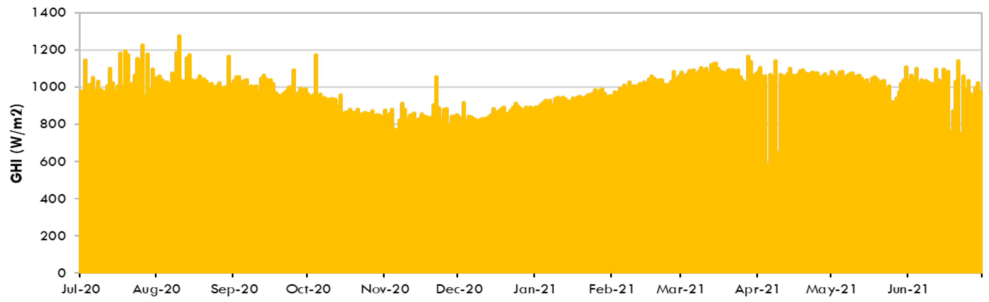
Figure 2.
Wind Potential map in Oman and wind avg. speed Source: Adapted from [15].
Figure 2.
Wind Potential map in Oman and wind avg. speed Source: Adapted from [15].
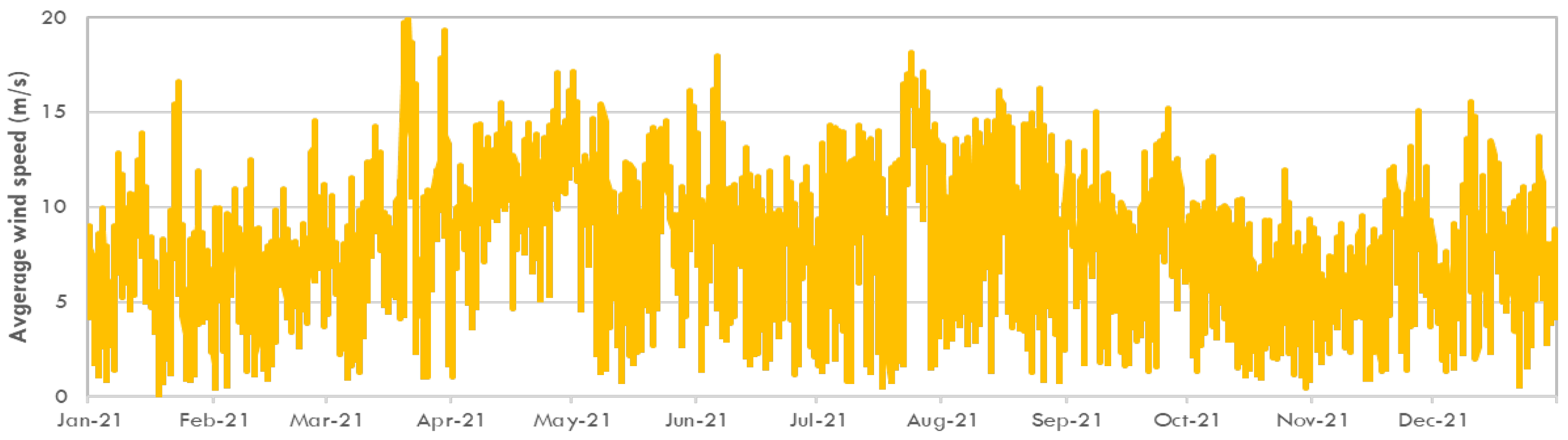
Chart 1.
Some key developments and initiatives in Oman related to energy transition and decarbonization Source: Author owns creation..
Chart 1.
Some key developments and initiatives in Oman related to energy transition and decarbonization Source: Author owns creation..
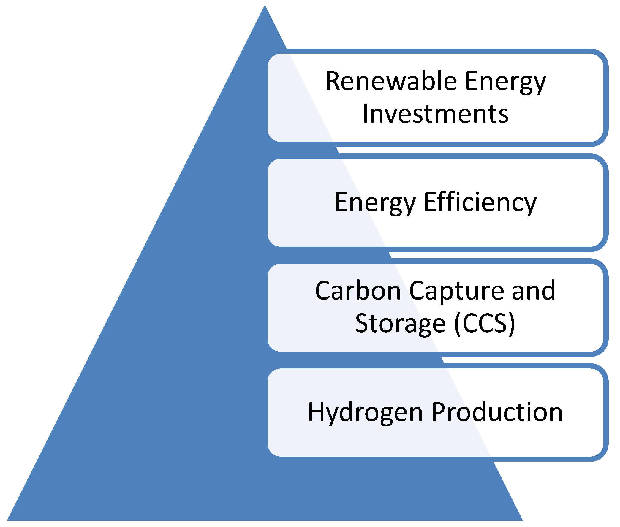
Figure 3.
Hodrick-Prescott Filter (Tambada = 100).
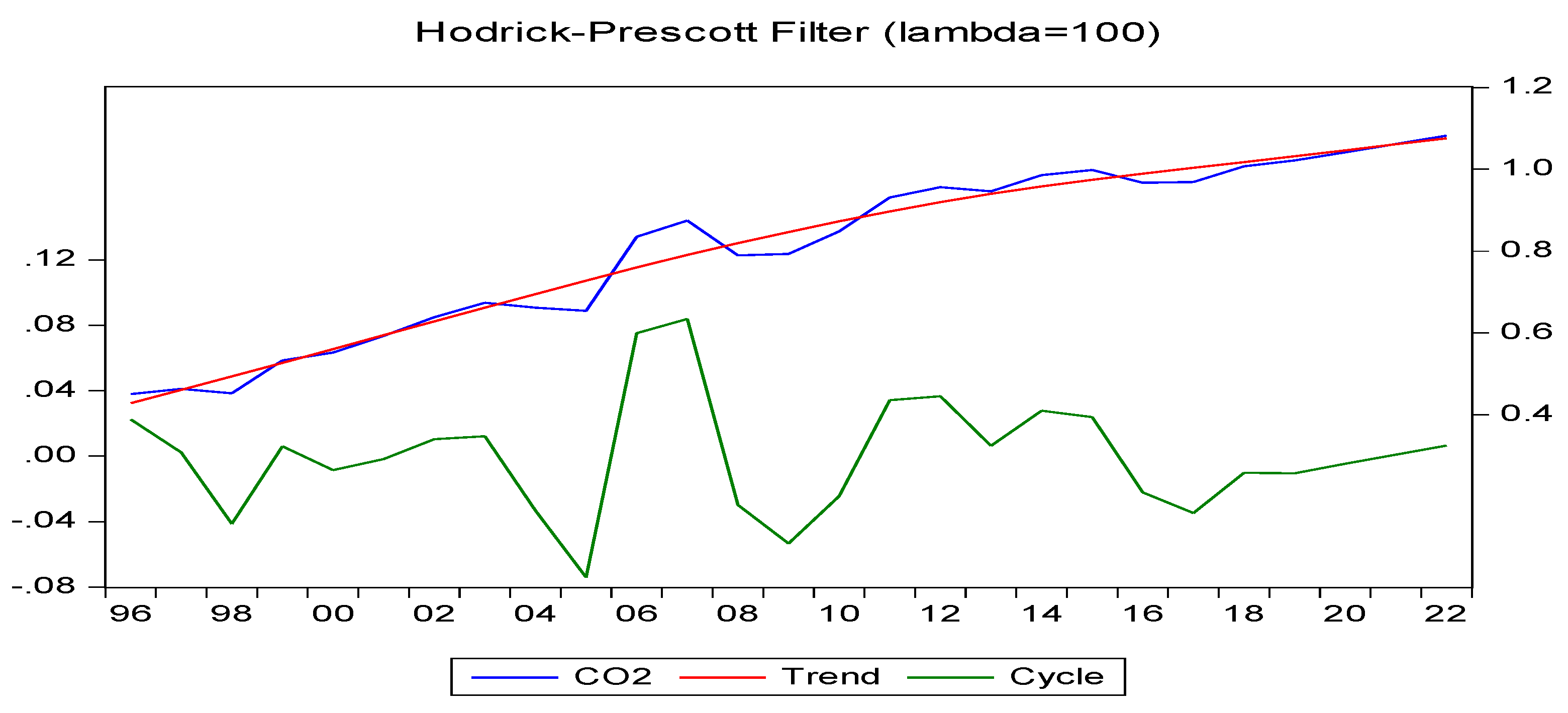
Figure 4.
Results of CUSUM and CUSUM square tests.
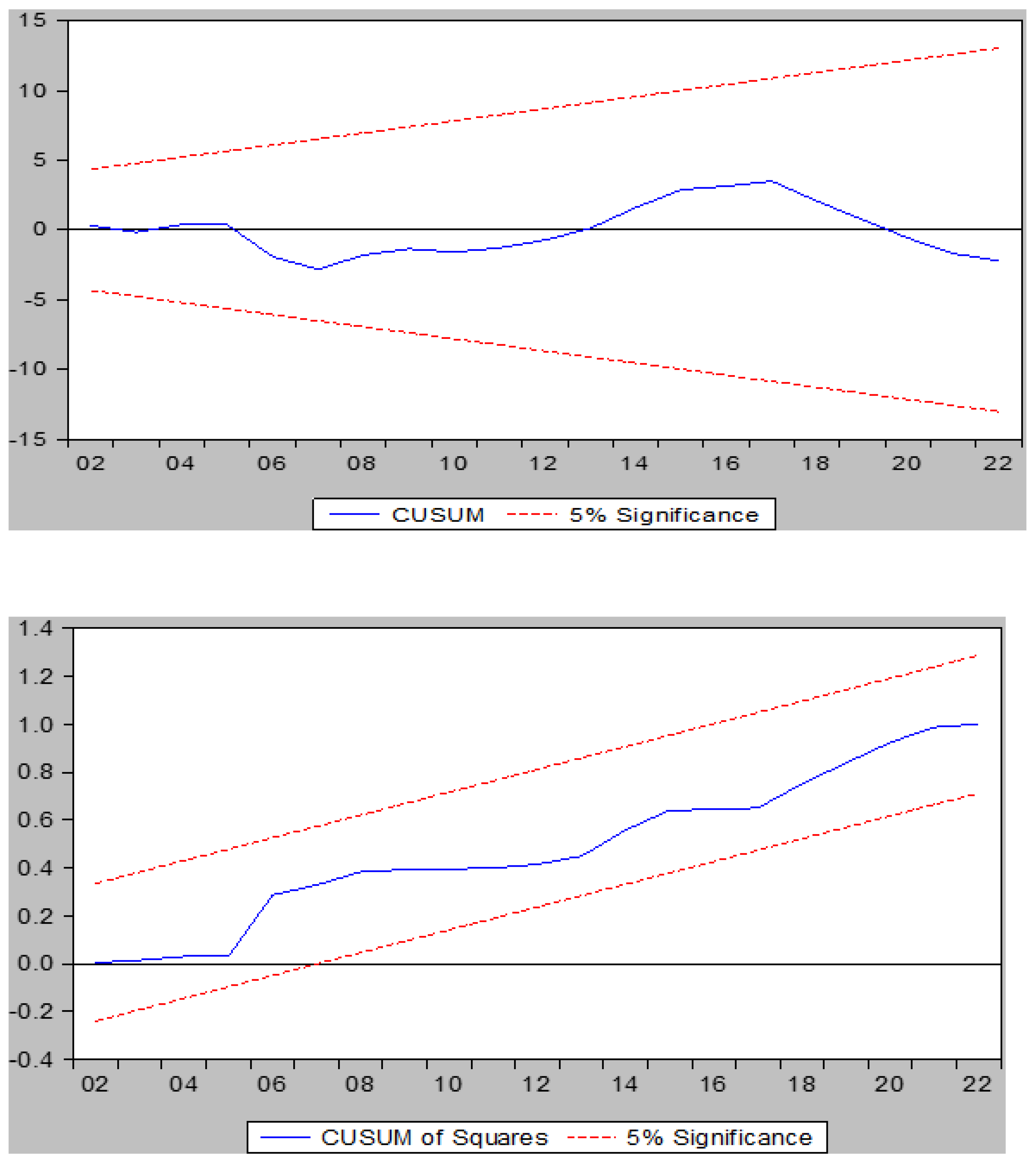
Figure 5.
Inverse of AR Characteristic Polynomial.
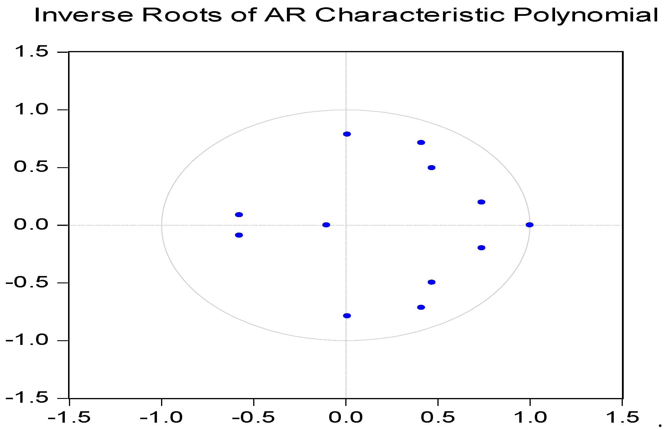

Table 1.
Variables’ description and data sources.
| Definition | Codes | Source | |
|---|---|---|---|
| Dependent variable | CO2 emissions (metric tons per capita) | CO2 | WDI, 2022 |
| Independent variables | Real GDP at constant 2011 national prices (Converted to the equivalent USD million, 2011) Energy use (kg of oil equivalent per capita) Urban Population |
RGDPCit ENGYit URBit |
PWT 10.0 WDI, 2022 WDI, 2022 |
| Control variables | Foreign Direct Investment (% of GDP) | FDIit | WDI, 2022 |
| Financial Development Index | FDX it | WDI, 2022 |
Source: [35]. The information was taken from PennWorld Table, 10.0, Available at: https://www.rug.nl/ggdc/ productivity/pwt/?lang=en accessed on 15 June 2024. ** World Bank, World development Indicators 23.
Table 2.
Summary of statistics for the model variables.
| Series | CO2 | FDX | ENGY | FDI | RGDPC | URB |
|---|---|---|---|---|---|---|
| Mean | 12.57616 | 41.99475 | 4691.028 | 2.002824 | 18599.18 | 75.64735 |
| Median | 13.28492 | 37.46007 | 5499.200 | 1.387658 | 18948.28 | 72.96700 |
| Maximum | 17.30974 | 77.32465 | 6771.205 | 7.917523 | 21458.39 | 87.91250 |
| Minimum | 6.566793 | 20.61221 | 2328.300 | -2.760018 | 13841.41 | 66.10200 |
| Std. Dev. | 3.583404 | 16.26026 | 1597.079 | 2.169683 | 1913.771 | 6.025801 |
| Skewness | -0.393347 | 0.701653 | -0.079602 | 0.737625 | -0.571905 | 0.700000 |
| Kurtosis | 1.600569 | 2.405329 | 1.214834 | 3.630601 | 2.672211 | 2.262357 |
| Probability | 0.170012 | 0.202504 | 0.109881 | 0.170394 | 0.377824 | 0.178783 |
| Sum | 415.0133 | 1385.827 | 154803.9 | 66.09319 | 613772.8 | 2496.363 |
| Sum Sq. Dev. | 410.9051 | 8460.676 | 81621140 | 150.6408 | 1.17E+08 | 1161.929 |
| C.V | 28.50% | 38.72% | 34.06% | 8.32% | 10.29% | 7.96% |
| Observations | 33 | 33 | 33 | 33 | 33 | 33 |
Table 3.
Stepwise Regression.
| Variable | Coefficient | Std. Error | t-Statistic | Prob. |
|---|---|---|---|---|
| FDX | -0.0203 | 0.0321 | -0.6326 | 0.5323 |
| ENGY | 0.0012 | 0.0003 | 4.0273 | 0.0004 |
| FDI | -0.0446 | 0.1053 | -0.4241 | 0.6749 |
| RGDPC | 0.0007 | 0.0002 | 4.2662 | 0.0002 |
| URB | 0.3449 | 0.135619 | 2.5438 | 0.017 |
| C | -30.823 | 10.3176 | -2.9874 | 0.0059 |
| R-squared | 0.9228 | Mean dependent var | 12.5762 | |
| Adjusted R-squared | 0.9086 | S.D. dependent var | 3.58340 | |
| S.E. of regression | 1.0836 | Akaike info criterion | 3.16147 | |
| Sum squared resid | 31.7048 | Schwarz criterion | 3.4336 | |
| Log likelihood | -46.1643 | Hannan-Quinn criter. | 3.2530 | |
| F-statistic | 64.5859 | Durbin-Watson stat | 2.0399 | |
Table 4.
Robust Least Squares.
| Variable | Coefficient | Std. Error | z-Statistic | Prob. |
|---|---|---|---|---|
| FDX | -0.021083 | 0.033512 | -0.629119 | 0.5293 |
| ENGY | 0.001320 | 0.000313 | 4.217142 | 0.0000 |
| FDI | -0.032617 | 0.109913 | -0.296754 | 0.7667 |
| RGDPC | 0.000630 | 0.000166 | 3.804982 | 0.0001 |
| URB | 0.331275 | 0.141597 | 2.339569 | 0.0193 |
| C | -29.55645 | 10.77239 | -2.743722 | 0.0061 |
| Robust Statistics | ||||
| R-squared | 0.704947 | Adjusted R-squared | 0.650307 | |
| Rw-squared | 0.950575 | Adjust Rw-squared | 0.950575 | |
| Akaike info criterion | 50.85702 | Schwarz criterion | 60.63514 | |
| Deviance | 25.15234 | Scale | 0.796405 | |
| Rn-squared statistic | 313.4801 | Prob(Rn-squared stat.) | 0.000000 | |
Table 5.
Unit root test (ADF) for the model variables.
| Variable | Level ADF Test Statistic | Level Critical Value (5%) | Level P-Value | Conclusion | First Difference ADF Test Statistic | First Difference Critical Value (5%) | First Difference P-Value | Conclusion |
|---|---|---|---|---|---|---|---|---|
| CO2 | -1.944 | -2.93 | 0.311 | I(0) | -5.23 | -2.93 | 0.0001 | I(1) |
| RGDPC | 0.66 | -2.93 | 0.859 | I(0) | -4.87 | -2.93 | 0.0002 | I(1) |
| ENGY | -1.387 | -2.93 | 0.589 | I(0) | -6.11 | -2.93 | 0.0000 | I(1) |
| FDI | -1.511 | -2.93 | 0.526 | I(0) | -3.74 | -2.93 | 0.0035 | I(1) |
| FDX | -0.239 | -2.93 | 0.931 | I(0) | -4.35 | -2.93 | 0.001 | I(1) |
| URB | 0.338 | -2.93 | 0.979 | I(0) | -3.27 | -2.93 | 0.0175 | I(1) |
Table 6.
Johansen cointegration test Output.
| Hypothesized | Trace | 0.05 | ||
| No. of CE(s) | Eigenvalue | Statistic | Critical Value | Prob.** |
| None * | 0.852152 | 141.5134 | 95.75366 | 0.0000 |
| At most 1 * | 0.697394 | 82.25467 | 69.81889 | 0.0037 |
| At most 2 | 0.412530 | 45.19960 | 47.85613 | 0.0870 |
| At most 3 | 0.345267 | 28.70978 | 29.79707 | 0.0663 |
| At most 4 * | 0.304168 | 15.58042 | 15.49471 | 0.0486 |
| At most 5 * | 0.130596 | 4.338355 | 3.841466 | 0.0373 |
Table 7.
Canonical Cointegrating Regression (CCR).
| Variable | Coefficient | Std. Error | t-Statistic | Prob. |
|---|---|---|---|---|
| FDX | -0.019669 | 0.031739 | -0.619717 | 0.5408 |
| FDI | -0.038942 | 0.113381 | -0.343464 | 0.734 |
| ENGY | 0.001324 | 0.000299 | 4.430817 | 0.0002 |
| RGDPC | 0.000698 | 0.000156 | 4.466309 | 0.0001 |
| URB | 0.286755 | 0.134713 | 2.128644 | 0.0429 |
| C | -27.48004 | 10.17604 | -2.700465 | 0.012 |
| R-squared | 0.912471 | Mean dependent var | 12.76395 | |
| Adjusted R-squared | 0.895639 | S.D. dependent var | 3.471841 | |
| S.E. of regression | 1.121577 | Sum squared resid | 32.70632 | |
| Durbin-Watson stat | 2.987638 | Long-run variance | 1.002499 | |
Table 8.
Engle -Granger Cointegration Test.
| Dependent | tau-statistic | Prob.* | z-statistic | Prob.* |
|---|---|---|---|---|
| CO2 | -3.428854 | 0.5736 | -24.59148 | 0.1746 |
| FDX | -4.102383 | 0.2905 | -36.11239 | 0.0043 |
| ENGY | -3.970701 | 0.3369 | -21.602 | 0.3232 |
| RGDPC | -3.454003 | 0.5621 | -21.81771 | 0.3021 |
| FDI | -3.498553 | 0.5404 | -18.35119 | 0.5185 |
| URB | -4.40806 | 0.1949 | -33.18668 | 0.0142 |
| *[37] p-values. | ||||
Table 9.
Vector Error Correction Estimates.
| Table 14: Vector Error Correction Estimates | |||||
| Cointegrating Eq: | CointEq1 | ||||
| FDX(-1) | 1.000000 | ||||
| ENGY(-1) | 0.012985 | ||||
| (0.00173) | |||||
| [ 7.51782] | |||||
| URB(-1) | -5.785633 | ||||
| (0.39863) | |||||
| [-14.5139] | |||||
| RGDPC(-1) | -0.006445 | ||||
| (0.00102) | |||||
| [-6.30697] | |||||
| FDI(-1) | -1.308321 | ||||
| (0.42086) | |||||
| [-3.10868] | |||||
| 458.9406 | |||||
| Error Correction: | D(FDX) | D(ENGY) | D(URB) | D(RGDPC) | D(FDI) |
| CointEq1 | -1.29361 | 1.558143 | 0.015515 | 10.58644 | 0.098716 |
| (0.30792) | (30.1303) | (0.01322) | (41.6090) | (0.12697) | |
| [-4.20118] | [ 0.05171] | [ 1.17334] | [ 0.25443] | [ 0.77750] |
Source: Author's Calculation.
Table 10.
Fully Modified Least Squares (FMOLS).
| Variable | Coefficient | Std. Error | t-Statistic | Prob. |
|---|---|---|---|---|
| FDX | -0.016306 | 0.030732 | -0.530564 | 0.6002 |
| ENGY | 0.001340 | 0.000292 | 4.587023 | 0.0001 |
| FDI | -0.056056 | 0.097270 | -0.576295 | 0.5694 |
| RGDPC | 0.000657 | 0.000170 | 3.869514 | 0.0007 |
| URB | 0.284912 | 0.139012 | 2.049551 | 0.0506 |
| C | -26.69682 | 10.96363 | -2.435035 | 0.0221 |
| R-squared | 0.915782 | Mean dependent var | 12.76395 | |
| Adjusted R-squared | 0.899586 | S.D. dependent var | 3.471841 | |
| S.E. of regression | 1.100165 | Sum squared resid | 31.46941 | |
| Durbin-Watson stat | 2.033042 | Long-run variance | 1.002499 | |
Table 11.
The results of diagnostic tests.
| Diagnostic probes | Coefficient | p-value | Conclusion |
|---|---|---|---|
| Jarque-Bera analysis | 0.0796 | 0.6214 | The residuals follow a normal distribution. |
| Breusch-Godfrey LM analysis | 1.3340 | 0.35428 | No serial correlation is present. |
| Breusch-Pagan-Godfrey analysis | 1.5601 | 0.4762 | Heteroscedasticity is absent. |
| Stability (CUSUMSQ) | Stable | Stable | The model is stable. |
| Ramsey RESET analysis | 1.3574 | 0.2259 | The model is accurately specified |
Disclaimer/Publisher’s Note: The statements, opinions and data contained in all publications are solely those of the individual author(s) and contributor(s) and not of MDPI and/or the editor(s). MDPI and/or the editor(s) disclaim responsibility for any injury to people or property resulting from any ideas, methods, instructions or products referred to in the content. |
© 2024 by the authors. Licensee MDPI, Basel, Switzerland. This article is an open access article distributed under the terms and conditions of the Creative Commons Attribution (CC BY) license (http://creativecommons.org/licenses/by/4.0/).
Copyright: This open access article is published under a Creative Commons CC BY 4.0 license, which permit the free download, distribution, and reuse, provided that the author and preprint are cited in any reuse.


