
Submitted:
02 September 2024
Posted:
03 September 2024
You are already at the latest version
Abstract
In this paper, we consider the synchronization of chaotic oscillators interconnected via a second order dynamic coupling. The design of the proposed coupling is inspired in the ancient synchronization experiment of synchronized pendulum clocks, as described by the Dutch scientist Christiaan Huygens more than three centuries ago. It is demonstrated that the coupled chaotic systems may exhibit not only complete synchronization, but also mixed synchronization—some states synchronize in anti-phase whereas other states synchronize in-phase. In fact, a transition from complete synchronization to mixed synchronization or viceversa can be induced by just changing a single parameter in the coupling. Additionally, the stability of the synchronous solution is investigated by using the Master Stability Function approach and the largest transverse Lyapunov exponent. The Lorenz system is considered as particular application example. Finally, the performance of the proposed synchronization scheme is illustrated with computer simulations and validated by means of experiments using electronic circuits.
Keywords:
Synchronization
; mixed-synchronization
; chaos
; Huygens’ coupling
; electronic circuit
1. Introduction
Synchronization—i.e. adjustment of rhythms to a certain pattern—is one of the most dominant behaviors in the universe. There are oscillating systems where synchronization occurs naturally, like for example biological systems, where it has been found that two or more cells, independently of their nature, or functioning, may synchronize by using signaling messengers (as for example light) as the coupling signal [1]. Furthermore, spontaneous synchronization may also emerge in inert systems. This is the case of, for example, pendulum clocks suspended from a common structure oscillating synchronously [2,3], metronomes placed on a wooden structure supported by soda cans moving in perfect synchrony [4], and in the arena of soft polymeric materials, liquid crystalline oscillators excited by light may exhibit in-phase and anti-phase motion [5].
In other cases, the synchronization phenomenon is artificially induced by, for instance, a control law. This kind of synchronization is called, for obvious reasons, controlled synchronization [6,7,8]. As an example, the reader may consider the coordination, formation and synchronization of robots and quadcopters [9,10,11,12,13], the synchronization of renewable energy-based hybrid micro-grids [14], or the synchronization of wireless network terminals, which are of vital importance in communication systems [15,16].
Synchronized behavior can also be observed in chaotic systems. Due to their sensitivity to initial conditions, these systems are not expected to synchronize in a natural way. However, it is possible to find suitable synchronizing schemes like drive-response configuration, bidirectional interconnection, or mutual coupling, such that two (or more) chaotic systems achieve synchronization [17].
Most of the existing synchronization schemes for chaotic systems are based on the so called-diffusive coupling, in which the oscillators interact through the weighted difference of (part of) their states [18,19]. This type of coupling can be further used in the context of networks for inducing different types of synchronous motion like, for example, cluster synchronization [20], explosive synchronization [21], generalized synchronization [22],chimera states [23], among others.
However, it has been observed that diffusive couplings may have some limitations like, for example, inducing synchronization only within a limited interval of coupling strength values, or even worst, this type of couplings may not suffice to synchronize the systems [24]. Therefore, some methodologies have been proposed in the literature in order to enhance the performance of this type of couplings. For example, it has been shown that the use of transient uncoupling, i.e., intermittent activation of the coupling each time the state of the system is within some region of the chaotic attractor, can enhance the synchronizability of the interconnected systems [25]. Another alternative to improve the performance of diffusive couplings is to add time delays to the interconnection, as shown in our previous work [26].
Likewise, an enhancement in the synchronizabilty of chaotic oscillators can be achieved by replacing the diffusive coupling by a dynamic interconnection—also referred to as environmental coupling in the literature—where the interaction between the oscillators is indirect via a dynamical system [27]. The power of dynamic coupling relies on the fact that it can be used for synchronizing chaotic and hyper-chaotic systems that are non synchronizable when using standard diffusive couplings, see. e.g. [28,29,30]. Also, for the case of networks, diffusive coupling may have a limitation in the maximum number of oscillators that can be synchronized. However, by using dynamic coupling, it is possible to synchronize a larger number of oscillators [31].
Consequently, in this paper, we further explore the use of dynamic couplings for synchronizing chaotic systems. Specifically, we consider a synchronization scheme, in which the systems do not interact directly (like in the classic master-slave configuration or bidirectional coupling), but rather through a linear second order dynamical system.
The design of the proposed coupling resembles the type of coupling used by Huygens for synchronizing his pendulum clocks, such that each chaotic system receives exactly the same coupling signal. Then, at first sight, it may not be intuitive to see why a common coupling signal can synchronize two chaotic systems, which are well-known to be extremely sensitive to initial conditions.
Through the analysis, we consider chaotic systems having a particular type of symmetry such that two types of synchronization are observed: complete synchronization and mixed synchronization, where part of the state variables synchronize in anti-phase whereas the rest of synchronize in-phase. In both cases, the stability of the synchronous solution is investigated by using the master stability function approach, and the obtained results are illustrated by means of computer simulations. Finally, an experimental study is conducted by using chaotic oscillators implemented in electronic circuits.
The outline of this paper is as follows. First, a brief description of the original Huygens’ coupling is presented in Section 2, whereas the proposed synchronization scheme and the corresponding problem description are presented in Section 3 . Next, the stability of the synchronous solutions in the coupled systems is investigated in Section 4, and an application example is presented in Section 5. Then, the obtained experimental results are summarized in Section 6. Finally, in Section 7, a discussion and some conclusions are provided.
2. Preliminaries: Huygens Coupling
One of the earliest scientific reports on spontaneous synchronization of inert systems dates back to the seventeen century, when the eminent scientist Christiaan Huygens observed—by serendipity—that two pendulum clocks were oscillating in harmony, at the same pace, but in opposite directions, a phenomenon baptized by Huygens as the symphaty of clocks. The peculiar experimental setup used by Huygens is shown in Figure 1(a). It consists of two pendulum clocks mounted on a wooden bar, which in turn is mounted on the top of two chairs. Through the years, several mathematical models have been derived in order to explain the synchronization phenomenon observed by Huygens [2,32,33,34].
For the modelling, most of the existing works consider the clocks as simple pendulums and the coupling structure is modelled as a rigid bar elastically attached to a fixed support, as shown in Figure Figure 1(b). Under these considerations, the mathematical model of Huygens experiment is given by the following set of equations:
where are the angular displacement of the pendulums, is the horizontal displacement of the coupling rigid bar, and are the mass, length and rotational damping of the pendulums, whereas are the mass, stiffness and damping coefficients, respectively, of the coupling bar. The external torques correspond to the escapement mechanism that is responsible of keeping the oscillations in the pendulum. It is the mechanism that produces the characteristic tic and toc in a mechanical clock.
Note that the coupling between the clocks, which is referred to as Huygens’ coupling in the literature, see e.g. [36], is a mass-spring-damper system described by a second order equation and thus it can be classified as a dynamic coupling. Another important observation is that both clocks are equally influenced by the coupling, i.e., the clocks receive the same signal , which corresponds to the acceleration of the coupling bar, as can be seen from the first two equations in (1).
Depending on the parameters of the coupling bar, the pendulums may synchronize in-phase or in anti-phase, among other limit solutions. In fact, in [37], the authors have shown that just by changing the mass of the coupling bar, it is possible to switch from in-phase synchronous motion to anti-phase synchronization and viceversa.
Inspired by this, in this work we want to address the following questions. Can we use Huygens’ coupling for synchronizing chaotic oscillators? If yes, would it be possible to switch between two different synchronous states by just changing a parameter in the coupling?
In what follows, we demonstrate that the answer to the aforementioned questions is affirmative.
3. Proposed Synchronization Scheme and Problem Description
The basic idea in this work is to apply Huygens’ coupling in the context of chaotic oscillators. Roughly speaking, we want to replace the pendulums in the schematic diagram of Figure 1(b) by chaotic oscillators, as shown in the block diagram of Figure 2, and to determine the possible synchronous behaviors.
Mathematically, the proposed coupling scheme is described by
where is the state vector of oscillator , is the state vector of the dynamic coupling, is the coupling strength, the matrices and determine, which variables of the oscillators and the dynamic coupling are used for the interconnection, is a binary parameter, i.e., , such that, as we will show later in Section 4, for complete synchronization, whereas for mixed synchronization. Furthermore, is a nonlinear function describing the intrinsic dynamics of the oscillators and matrix is given by
where are the dimensionless damping and natural frequency, respectively, of the dynamic coupling. It is well-known, see e.g. [38], that the dimensionless parameter determines the transient response of system (4) when : underdamped for , critically damped for , and overdamped for .
Through this work, we are interested in a particular class of chaotic oscillators namely, systems that have an especial axial symmetry such that the coupled systems not only achieve complete synchronization but also, the so called mixed synchronization, where part of the state variables synchronizes in anti-phase, whereas the rest of variables are fully synchronized. Our ultimate goal is to show that, by changing one single parameter in the proposed dynamic coupling, two different types of synchronous behavior can be observed, just as is the case in the original Huygens’ experiment of synchronized pendulum clocks.
Consequently, the state of the oscillators is partitioned as follows
where , , is the part of the state that can synchronize either in-phase or in anti-phase, whereas , contains the variables that only can synchronize in-phase.
According to the above state partition, the function and the coupling vectors and are also partitioned as follows
where , , , , , .
Then, the following assumption is required
- A1
- The uncoupled system, i.e., , is invariant under the transformation
Note that this assumption implies that the functions and satisfy
Furthermore, from the results presented in [39], it follows that assumption 1 guarantees the existence of the mixed synchronous solution.
Now, we are ready to provide the following definitions.
Definition 1
(Complete Synchronization). The coupled system (2)-(4) is said to achieve complete synchronization if
Definition 2
(Mixed Synchronization). The coupled system (2)-(4) is said to achieve mixed synchronization if
Note that in both definitions, it is required that the effect of the coupling signal vanishes, i.e., the coupling should be noninvasive in the sense that, its influence disappears once the oscillators are synchronized.
4. Stability Analysis
In this section we use the Master Stability Function approach in order to investigate the stability of the synchronous solutions (10) and (11).
4.1. Complete Synchronization
We start by analyzing the stability of the synchronous solution (10).
The first step is to linearize system (2)-(4) around the solution and , where is the solution of an isolated node, i.e., is the solution of the system . Furthermore, we consider .
This yields the following variational equation
where , , and is the Jacobian of function .
Next, we define the following errors for complete synchronization
Therefore, we obtain the following variational equation for the synchronization error
4.2. Mixed Synchronization
Next, we derive a variational equation for determining the local stability of the mixed synchronous solution (11). In this case, it is convenient to rewrite system (2)-(4) using the partitions (6)-(7), considering , and defining . Furthermore, we also assume that the coupling in Eq. (4) is only through the variables, i.e., we consider . Under these considerations, system (2)-(4) is rewritten as follows
Next, from Eq. (9) we have that and Taking this into account and linearizing the resulting system around the solution , and , where as before, corresponds to the solution of an isolated node, we obtain the following variational equation
where , , , , and the partial derivatives are given in Eqs. (A1)-(A8) in Appendix A.
Finally, the following errors for mixed synchronization are defined
Therefore, the resulting variational equation for the mixed synchronization solution is given by
where we have used the fact that ,
, , . Furthermore and are zero matrices.
5. Application Example
Now, we illustrate the performance of the proposed coupling scheme (2)-(4). To this end, we consider a pair of chaotic Lorenz systems.
For the sake of example, we choose the following coupling matrices
where . For this choice, the dynamic coupling will be applied to the first equation of each Lorenz oscillator.
Then, system (2)-(4) takes the following explicit form
where are the state variables of oscillator i, for , and the state variables of the Huygens’ coupling are given by .
Note that each uncoupled oscillator is invariant under the transformation , i.e., Assumption , see Eq. (8), is satisfied. Thus, it is expected that both complete and mixed synchronization exist in the coupled system (30)-(32).
Now, we investigate the stability of the synchronous solutions (10) and (11) in the coupled system (30)-(32). As a first step, we have found that, for this example, the variational equation (16) corresponding to complete synchronization and the variational equation (28) corresponding to the mixed synchronous solution, are equal, i.e.,
where and correspond to the trajectories of an isolated Lorenz system.
The next step is to compute the largest transverse Lyapunov exponent either from Eqs. (16)-(33) or from Eqs. (28)-(33). In this case it does not matter which equation we use for the stability analysis, since for this particular case both equations are identical as mentioned above. For the computation of , we use the Wolf algorithm [40] and the following parameter values: , which are the standard values for the Lorenz system, and, for the dynamic coupling, we take and . With this, the largest transverse Lyapunov exponent is computed as a function of the coupling strength k and parameter , both are varied in the interval in steps of 0.5. The obtained results are shown in Figure 3(a), where the green colors indicates the areas where is negative and therefore, in that region of the ()-plane, the complete synchronous solution is locally stable for , whereas the mixed synchronization solution is locally stable for . Different green tones are used to indicate how negative is . On the other hand, in the red region, is positive and thus, for that combination of values of the synchronous solution, either complete synchronization or mixed synchronization, is unstable.
In order to validate the stability regions shown in Figure 3(a), we numerically integrate system (30)-(32) using the Runge Kutta method, with step size of 0.001, and the same parameter values used for generating Figure 3. The system response is studied as a function of the scaling factor and the coupling strength k. Again, is varied in the interval and is varied in the interval , both in steps of 0.25, and we set . Moreover, the initial conditions used in the analysis are . The obtained results are shown in Figure 3(b). The blue color indicates the region where the oscillators achieve complete synchronization, whereas the orange area indicates the region where the oscillators do not synchronize. Exactly the same graph is obtained if is changed to . However, in such case, the blue color will indicate the region of mixed synchronization and again the orange region will correspond to unsynchronized behavior.
We can see that there is a complete agreement between the predicted stability regions and the numerical simulations shown in Figure 3. The red region in panel (a), where corresponds to the orange region in panel (b), where the oscillators behave unsynchronized. Likewise, the green areas on panel (a), where coincide with the blue are on panel (b), where the oscillators achieve synchronization in the simulation.
Note that the results presented in Figure 3 correspond to a particular choice of and , which are parameters of the Huygens coupling, see Eq. (5). However, a natural question at this point is how the choice of these parameters affects the stability of the synchronous solution. To see this, we compute , as a function of the coupling strength and these parameters. First, from Figure 3(a), we chose a value of within the lemon green region, for example . Then, using the same parameter values as used in Figure 3, we compute from from Eqs. (16)-(33) as a function of k and . The obtained results are shown in Figure 4(a). We can see that is more negative around the interval .
Also, for large values of a larger coupling strength k is required for making stable the synchronous solution.
Next, we fix the value of in and we compute again but this time as a function of k and . The results are depicted in Figure 4(b). It can be seen that an optimal value of , for which the largest transverse Lyapunov exponent is more negative is .
Thus, in summary, from the results presented in Figures (Figure 3) and (Figure 4) we can conjecture that, for the coupled system (30)-(32) and the considered parameter values, an optimal choice (optimal in the sense that the resulting is more negative) of the parameters of the dynamic coupling is: and .
In a second numerical study, we analyze the case where the interaction between the Lorenz oscillators is via the third variable. Hence, the coupling matrices in are selected as follows
The variational equation for the case of complete synchronization, i.e., , is as given in Eq. (16) with
Remark 1.
Note that, in this particular example, it is possible to observe both complete and mixed synchronization,withoutchanging the value of β. The reason of this is because, the variational equation of the mixed and complete synchronous behavior, for , are the same.
Now, we compute the largest transverse Lyapunov exponent from Eq. (16)-(35), as a function of the coupling strength k and parameter . The parameter values of the Lorenz oscillators are the same as used in the studies above, whereas the parameter values of the coupling system are set to and .
The obtained results are shown in Figure 5, where it can be seen that there is a small region in the ()-plane (green are) where the is negative and consequently, the synchronous solution either complete synchronization or mixed synchronization is locally stable.
From Remark 1, it follows that without changing any parameter in the system, it may be possible to observe the so called multistability, i.e., different stable behaviors may be observed, depending on the initial conditions. To show this, we numerically integrate system (2)-(4) with the coupling vectors given in (34). The parameter values of the Lorenz system are the same used so far, i.e., , and . For the Huygens coupling the parameters are and and the coupling strength k and are chosen from the green region in the plane shown in Figure 5. We choose and . Furthermore, we use the Runge-Kutta method with step size of 0.001 and the initial conditions are varied in the interval in steps of 0.1 and the rest of initial conditions are all set to zero.
The obtained numerical results are shown in Figure 6, from which the multistability of solutions becomes evident. Specifically, from that figure we can distinguish three behaviors: complete synchronization (blue), mixed synchronization (yellow) and a nonhomogeneous equilibrium solution (red lines on the axes), where the oscillators converge to an unsynchronized equilibrium point.
6. Experimental Results
Finally, in this section, the performance of the proposed synchronization scheme based on Huygens’ coupling is experimentally demonstrated. To this end, system (30)-(32) is physically implemented with analog electronic circuits.
As a first step, system (30)-(32) is scaled by introducing an attenuation factor such that , , , , for .
Furthermore, the system is also scaled in time by introducing the transformation , where is a dimensionless time and .
As a next step in the design of the circuit, the parameters in the above system are rewritten in terms of resistors and capacitors.
This yields
This is the system of equations that we use for electronic implementation using analog circuits, including resistors, capacitors, multipliers and operational amplifiers.
The schematic diagram of the circuit is shown in Figure 7, whereas the circuit for the Huygens’ coupling is depicted in Figure 8. In these diagrams, switch 1 (SW1) has been added with the purpose of coupling or decoupling the systems, i.e. when SW1 is in position 2, the systems are coupled, otherwise the systems are uncoupled or isolated.
On the other hand, switch 2 (SW2) is indeed the parameter . For , i.e. mixed synchronization, switch SW2 in the diagram of Figure 7 should be in position 1, whereas the switch SW2 in Figure 8 should be in position 2. On the other hand, for , i.e., for complete synchronization, the positions of the switches SW2 mentioned before have to be reversed.
For the experiments, we consider the components and values that are summarized in Table 1. These parameter values correspond to the following parameter values in the scaled system (38)-(43): and . For these values, mixed and also complete synchronization are expected to be stable.
The obtained experimental results, for the case of mixed synchronization, are shown in Figure 9, Figure 10 and Figure 11. The time series are recorded using a Teledyne Lecroy oscilloscope. As can be seen, besides the unavoidable (small) differences in the components of the circuit, the variables (voltages) and are in anti-phase, see Figure 9, the variables and are also in anti-phase, as shown in Figure 10, whereas the and variables are in complete synchrony, see Figure 11. Thus, the circuit exhibits the desired mixed synchronization behavior according to Definition 2, see Eq. (11).
When is switched to , the circuit achieves complete synchrony (for the sake of brevity and length of the paper, these experiments are not included).
These experimental results are in good agreement with the numerical results presented in Section 5. Note, however, that due to the fact that in the physical implementation the systems are inherently non identical, what we really observe in the experiments is the so-called practical synchronization [41]. This can be seen, for instance, from the phase planes shown in the above figures, where we can observe that the diagonal line is a bit tick, indicating that perfect synchrony is not achieved but rather practical synchronization is achieved. Nevertheless, the experimental results are more than satisfactory and nicely illustrate and validate the performance of Huygens’ coupling.
7. Discussion and Conclusions
A novel coupling strategy for synchronizing a pair of chaotic systems has been presented, which is inspired in the old synchronization experiment of pendulum clocks reported by Huygens on the 17th century. Just as in Huygens experiment, we have demonstrated that if the chaotic systems satisfy a symmetry condition, it is possible to observe at least two types of synchronous motion namely, complete synchronization and mixed synchronization. Furthermore, we have evaluated the performance of the proposed coupling using electronic circuits. A remarkable characteristic of the proposed coupling is that both oscillators receive exactly the same coupling signal and that the interaction between the oscillators is indirect.
The numerical study conducted for the case of Lorenz systems has shown that for certain choice of coupling matrices, transitions from complete synchronization to mixed synchronization and viceversa may be achieved by just changing a parameter in the coupling, whereas for other choices, we may observe multistability, i.e., without any change in the coupling, the systems may exhibit different synchronous behavior by just changing the initial conditions.
Here, we have applied the proposed coupling scheme to chaotic systems. However, it is our believe that it can be applied to a more general class of systems. Also, it would be interesting to compare the performance of our coupling strategy to other coupling schemes, like schemes based on diffusive coupling in order to determine possible advantages or disadvantages. This, however, is the topic of our ongoing research.
Author Contributions
Conceptualization, J.P. and A.A.; methodology, J.P. and A.A. and H.J.E.; software, R.D.M. and H.J.E.; validation, J.P, A.A, R.D.M and H.J.E; formal analysis, J.P, A.A, R.D.M and H.J.E; resources, R.D.M. and H.J.E.; data curation, J.P, A.A, R.D.M and H.J.E; writing—original draft preparation, J.P, A.A, R.D.M and H.J.E; writing—review and editing, J.P, A.A, R.D.M and H.J.E; visualization, R.D.M. and H.J.E.; supervision, J.P. and A.A.; project administration, J.P. and A. A.; funding acquisition, J.P. and H.J.E. All authors have read and agreed to the published version of the manuscript.
Funding
This research was partly funded by CONAHCYT and by the University of Guanajuato.
Data Availability Statement
The raw data supporting the conclusions of this article will be made available by the authors on request.
Conflicts of Interest
The authors declare no conflicts of interest.
Appendix A
Appendix A.1
References
- Kim, J.R.; Shin, D.; Jung, S.H.; Heslop-Harrison, P.; Cho, K.H. A design principle underlying the synchronization of oscillations in cellular systems. Journal of Cell Science 2010, 123, 537–543. [CrossRef]
- Bennett, M.; Schatz, M.F.; Rockwood, H.; Wiesenfeld, K. Huygens’s clocks. Proceedings of the Royal Society of London. Series A: Mathematical, Physical and Engineering Sciences 2002, 458, 563–579. [CrossRef]
- Pena Ramirez, J.; Olvera, L.; Nijmeijer, H.; Alvarez, J. The sympathy of two pendulum clocks: beyond Huygens’ observations. Scientific Reports 2016, 6. doi:10.1038/srep23580. [CrossRef]
- Pantaleone, J. Synchronization of metronomes. American Journal of Physics 2002, 70, 992–1000. [CrossRef]
- Vantomme, G.; Elands, L.; Gelebart, A.; Meijer, E.; . Pogromsky, A.; Nijmeijer, H.; Broer, D. Coupled liquid crystalline oscillators in Huygens’ synchrony. Nature Materials 2021, 20, 1702–1706. [CrossRef]
- Nijmeijer, H. A dynamical control view on synchronization. Physica D: Nonlinear Phenomena 2001, 154, 219–228. [CrossRef]
- Blekhman, I.; Fradkov, A.; Tomchina, O.; Bogdanov, D. Self-synchronization and controlled synchronization: general definition and example design. Mathematics and Computers in Simulation 2002, 58, 367–384. [CrossRef]
- Zhou, Z.; Gao, J.; Zhang, L. Synchronization Control with Dynamics Compensation for Three-Axis Parallel Motion Platform. Actuators 2024, 13. [CrossRef]
- Pérez-Fuentevilla, J.G.; Morales-Díaz, A.B.; Rodríguez-Ángeles, A. Synchronization Control for a Mobile Manipulator Robot (MMR) System: A First Approach Using Trajectory Tracking Master–Slave Configuration. Machines 2023, 11. [CrossRef]
- Xia, Y.; Hu, Z.; Wei, D.; Chen, K.; Peng, Y.; Yang, M. Biomimetic Synchronization in Biciliated Robots. Phys. Rev. Lett. 2024, 133, 048302. [CrossRef]
- Dallard, A.; Benallegue, M.; Kanehiro, F.; Kheddar, A. Synchronized Human-Humanoid Motion Imitation. IEEE Robotics and Automation Letters 2023, 8, 4155–4162. [CrossRef]
- Gudeta, S.G.; Karimoddini, A.; Yahi, N. Consensus-Based Distributed Collective Motion of Swarm of Quadcopters. IEEE Internet of Things Journal 2024, 11, 5184–5199. [CrossRef]
- Gastelum-Juarez, D.; Martha López-Gutiérrez, R.; Arellano-Delgado, A.; Cruz-Hernández, C. Outer Synchronization and Formation of Two Complex Heterogeneous Robotic Networks with an Intermediary Dynamic System. 2023 XXV Robotics Mexican Congress (COMRob), 2023, pp. 80–86. [CrossRef]
- Sahoo, S.C.; Barik, A.K.; Das, D.C. Synchronized voltage-frequency regulation in sustainable microgrid using novel Green Leaf-hopper Flame optimization. Sustainable Energy Technologies and Assessments 2022, 52, 102349. [CrossRef]
- Romanov, A.M.; Gringoli, F.; Sikora, A. A Precise Synchronization Method for Future Wireless TSN Networks. IEEE Transactions on Industrial Informatics 2021, 17, 3682–3692. [CrossRef]
- Son, W.; Choi, J.; Park, S.; Lee, H.; Jung, B.C. A Time Synchronization Protocol for Barrage Relay Networks. Sensors 2023, 23. [CrossRef]
- Fujisaka, H.; Yamada, T. Stability Theory of Synchronized Motion in Coupled-Oscillator Systems: . Progress of Theoretical Physics 1983, 69, 32–47. [CrossRef]
- Pecora, L.M.; Carroll, T.L. Synchronization of chaotic systems. Chaos: An Interdisciplinary Journal of Nonlinear Science 2015, 25, 097611. [CrossRef]
- Zhao, L.h.; Wen, S.; Li, C.; Shi, K.; Huang, T. A Recent Survey on Control for Synchronization and Passivity of Complex Networks. IEEE Transactions on Network Science and Engineering 2022, 9, 4235–4254. [CrossRef]
- Wang, Y.; Wang, L.; Fan, H.; Wang, X. Cluster synchronization in networked nonidentical chaotic oscillators. Chaos: An Interdisciplinary Journal of Nonlinear Science 2019, 29, 093118. [CrossRef]
- Muthanna, Y.A.; Jafri, H.H. Explosive transitions in coupled Lorenz oscillators. Phys. Rev. E 2024, 109, 054206. [CrossRef]
- LIU, J.; CHEN, G.; ZHAO, X. Generalized Synchronization and parameters identification of different-dimensional chaotic systems in the complex field. Fractals 2021, 29, 2150081. [CrossRef]
- Khatun, A.A.; Jafri, H.H. Chimeras in multivariable coupled Rössler oscillators. Communications in Nonlinear Science and Numerical Simulation 2021, 95, 105661. [CrossRef]
- Huang, L.; Chen, Q.; Lai, Y.C.; Pecora, L.M. Generic behavior of master-stability functions in coupled nonlinear dynamical systems. Phys. Rev. E 2009, 80, 036204. [CrossRef]
- Schröder, M.; Mannattil, M.; Dutta, D.; Chakraborty, S.; Timme, M. Transient Uncoupling Induces Synchronization. Phys. Rev. Lett. 2015, 115, 054101. [CrossRef]
- Márquez-Martínez, L.; Cuesta-García, J.; Pena Ramirez, J. Boosting synchronization in chaotic systems: Combining past and present interactions. Chaos, Solitons & Fractals 2022, 155, 111691. [CrossRef]
- Katriel, G. Synchronization of oscillators coupled through an environment. Physica D: Nonlinear Phenomena 2008, 237, 2933–2944. [CrossRef]
- Pena Ramirez, J.; Arellano-Delgado, A.; Nijmeijer, H. Enhancing master-slave synchronization: The effect of using a dynamic coupling. Phys. Rev. E 2018, 98, 012208. [CrossRef]
- Buscarino, A.; Fortuna, L.; Patanè, L. Master-slave synchronization of hyperchaotic systems through a linear dynamic coupling. Phys. Rev. E 2019, 100, 032215. [CrossRef]
- Arena, P.; Buscarino, A.; Fortuna, L.; Patanè, L. Lyapunov approach to synchronization of chaotic systems with vanishing nonlinear perturbations: From static to dynamic couplings. Phys. Rev. E 2020, 102, 012211. [CrossRef]
- de Jonge, W.; Ramirez, J.P.; Nijmeijer, H. Dynamic coupling enhances network synchronization ⁎⁎Partially supported by CONACYT Mexico. IFAC-PapersOnLine 2019, 52, 610–615. [CrossRef]
- Kapitaniak, M.; Czolczynski, K.; Perlikowski, P.; Stefanski, A.; Kapitaniak, T. Synchronization of clocks. Physics Reports 2012, 517, 1–69. [CrossRef]
- Goldsztein, G.H.; Nadeau, A.N.; Strogatz, S.H. Synchronization of clocks and metronomes: A perturbation analysis based on multiple timescales. Chaos: An Interdisciplinary Journal of Nonlinear Science 2021, 31, 023109. [CrossRef]
- Willms, A.R.; Kitanov, P.M.; Langford, W.F. Huygens’ clocks revisited. Royal Society Open Science 2017, 4, 170777. [CrossRef]
- Pena Ramirez, J.; Fey, R.H.B.; Nijmeijer, H. Synchronization of weakly nonlinear oscillators with Huygens’ coupling. Chaos: An Interdisciplinary Journal of Nonlinear Science 2013, 23, 033118. [CrossRef]
- Pena Ramirez, J.; Fey, R.H.B.; Nijmeijer, H. Synchronization of weakly nonlinear oscillators with Huygens’ coupling. Chaos: An Interdisciplinary Journal of Nonlinear Science 2013, 23, 033118. [CrossRef] [PubMed]
- Oud, W.; Nijmeijer, H.; Pogromsky, A. Experimental results on Huygens synchronization. IFAC Proceedings Volumes 2006, 39, 113–118. [CrossRef]
- Belykh, V.N.; Belykh, I.V.; Hasler, M. Hierarchy and stability of partially synchronous oscillations of diffusively coupled dynamical systems. Phys. Rev. E 2000, 62, 6332–6345. [CrossRef]
- Belykh, V.N.; Belykh, I.V.; Hasler, M. Hierarchy and stability of partially synchronous oscillations of diffusively coupled dynamical systems. Phys. Rev. E 2000, 62, 6332–6345. [CrossRef]
- Wolf, A.; Swift, J.B.; Swinney, H.L.; Vastano, J.A. Determining Lyapunov exponents from a time series. Physica D: Nonlinear Phenomena 1985, 16, 285–317. [CrossRef]
- Panteley, E.; Loría, A.; Conteville, L. On practical synchronization of heterogeneous networks of nonlinear systems: application to chaotic systems. 2015 American Control Conference (ACC), 2015, pp. 5359–5364. [CrossRef]
Figure 1.
Huygens’ setup of pendulum clocks. (a) Original Huygens’ drawing as appears in his laboratory notebook [35]. (b) Schematic representation.
Figure 1.
Huygens’ setup of pendulum clocks. (a) Original Huygens’ drawing as appears in his laboratory notebook [35]. (b) Schematic representation.
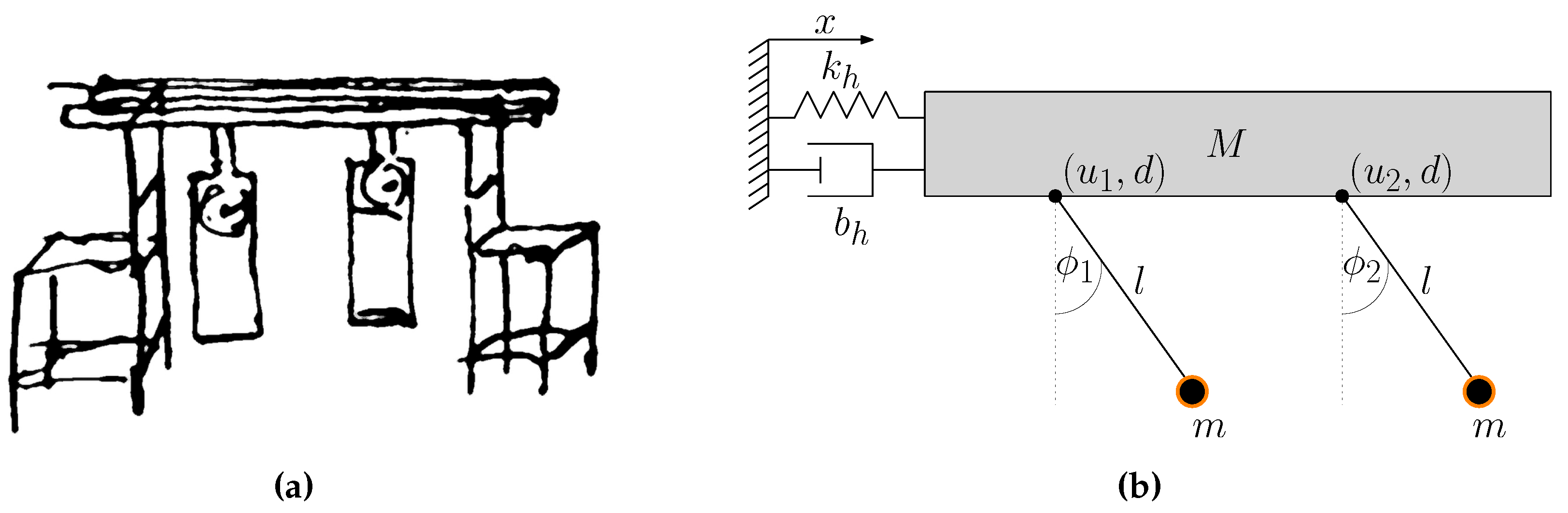
Figure 2.
Proposed synchronization scheme based on Huygens’ coupling.
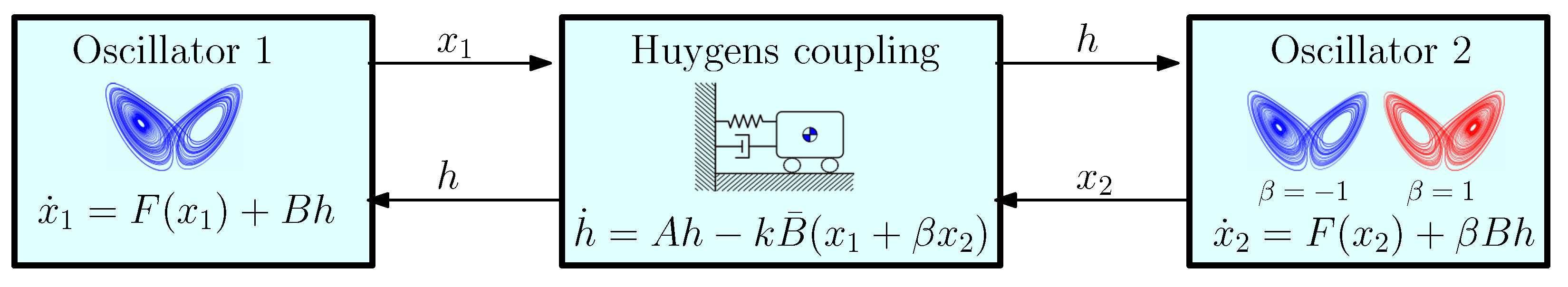
Figure 3.
The panel on the left is the stability chart, which shows the value of computed either from Eqs. (16)-(33) or from Eqs. (28)-(33). Green: and thus the corresponding synchronous solution is stable. Red: and consequently, the synchronous solution is unstable. In the lemon green area, is more negative and thus, it would be convenient to choose values of k and within this region. On the other hand, the panel on the left shows the simulation results obtained by numerical integration of Eqs. (30)-(32) for either (mixed synchronization) or (complete synchronization). Blue: Complete synchronization if or mixed synchronization if . Orange: Unstable behavior.Note that the red region in the left panel should be associated to the orange region in the right panel. Likewise, the green areas in the left panel should be compared to the blue are in the right panel. As can be seen, there is a clear agreement between the predicted stability regions (left) and the obtained numerical results (right).
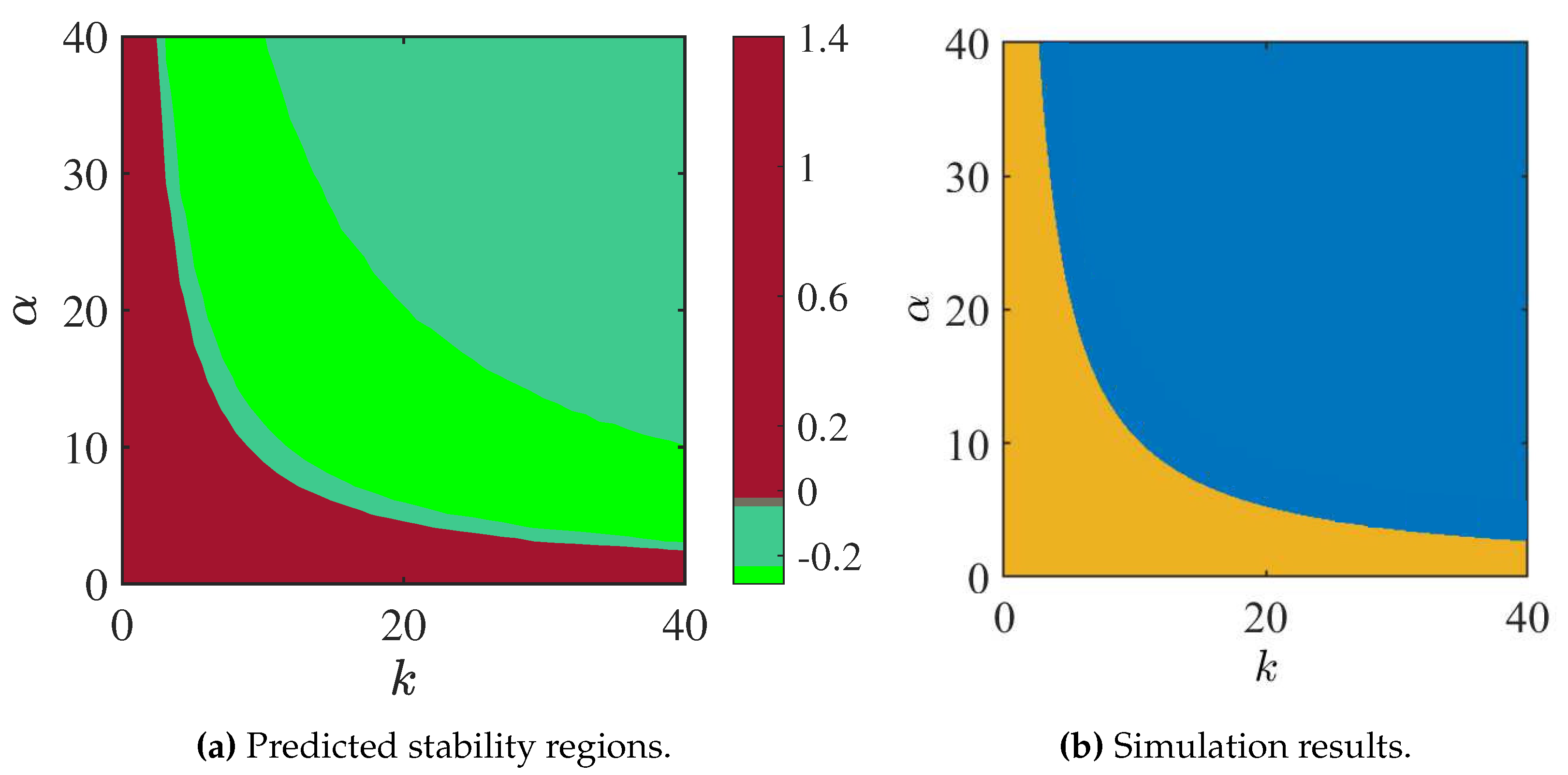
Figure 4.
Largest transverse Lyapunov exponent computed as a function of and . A possible ‘optimal’ choice is to take values of and k, for which is more negative.
Figure 4.
Largest transverse Lyapunov exponent computed as a function of and . A possible ‘optimal’ choice is to take values of and k, for which is more negative.
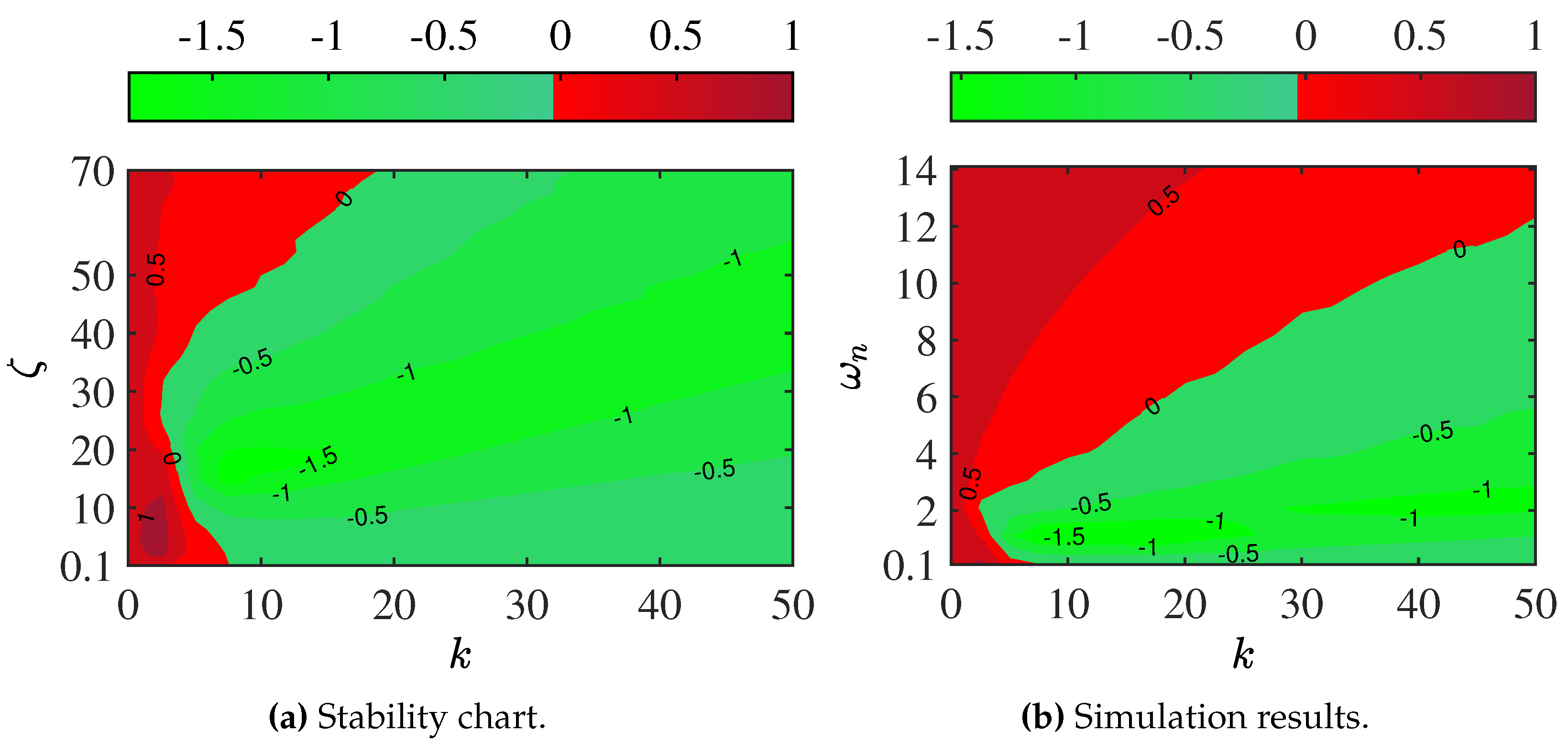
Figure 5.
Largest transverse Lyapunov exponent for system (6)-(35), as a function of the coupling strength k and parameter .
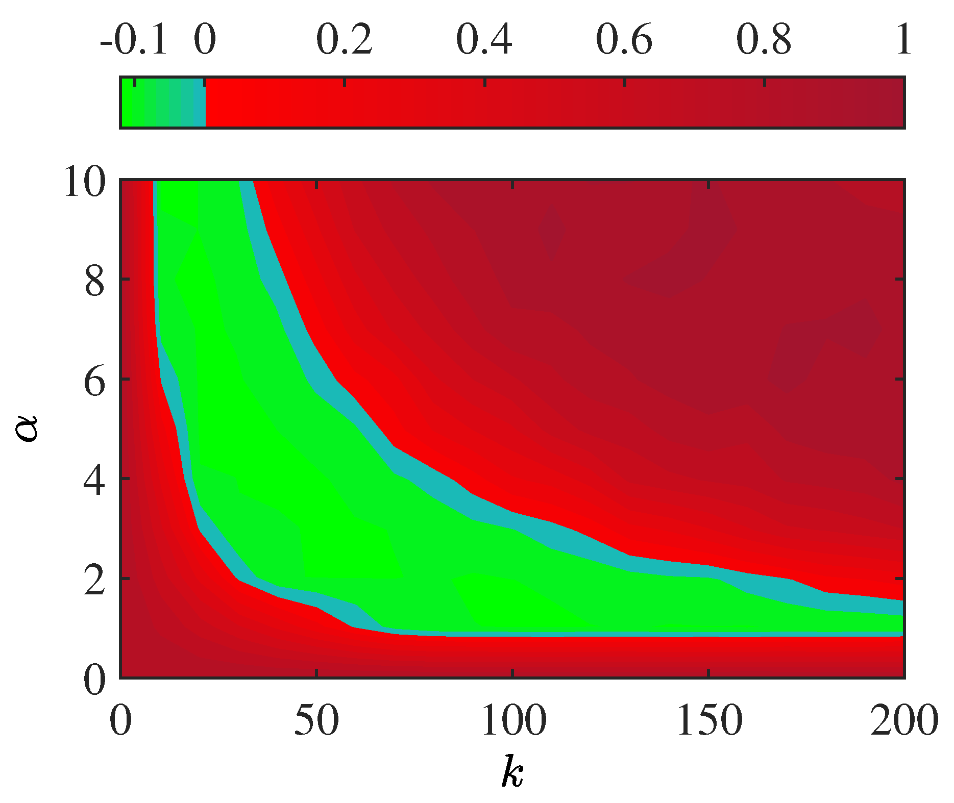
Figure 6.
Limit behavior of a pair of chaotic Lorenz systems, with the coupling vectors given in (34), as a function of the initial conditions and . Yellow: mixed synchronization. Blue: complete synchronization. Red: convergence to an unsynchronized equilibrium.
Figure 6.
Limit behavior of a pair of chaotic Lorenz systems, with the coupling vectors given in (34), as a function of the initial conditions and . Yellow: mixed synchronization. Blue: complete synchronization. Red: convergence to an unsynchronized equilibrium.
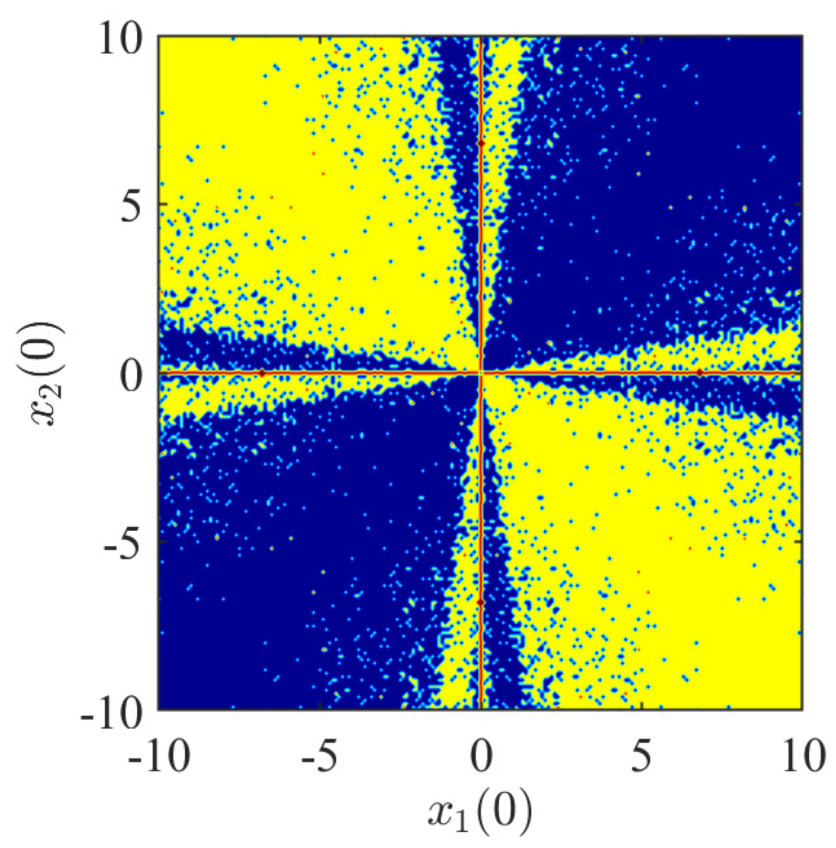
Figure 7.
Schematic diagram of the electronic circuit for implementing a pair of Lorenz systems from Eqs. (46)-(49).
Figure 7.
Schematic diagram of the electronic circuit for implementing a pair of Lorenz systems from Eqs. (46)-(49).
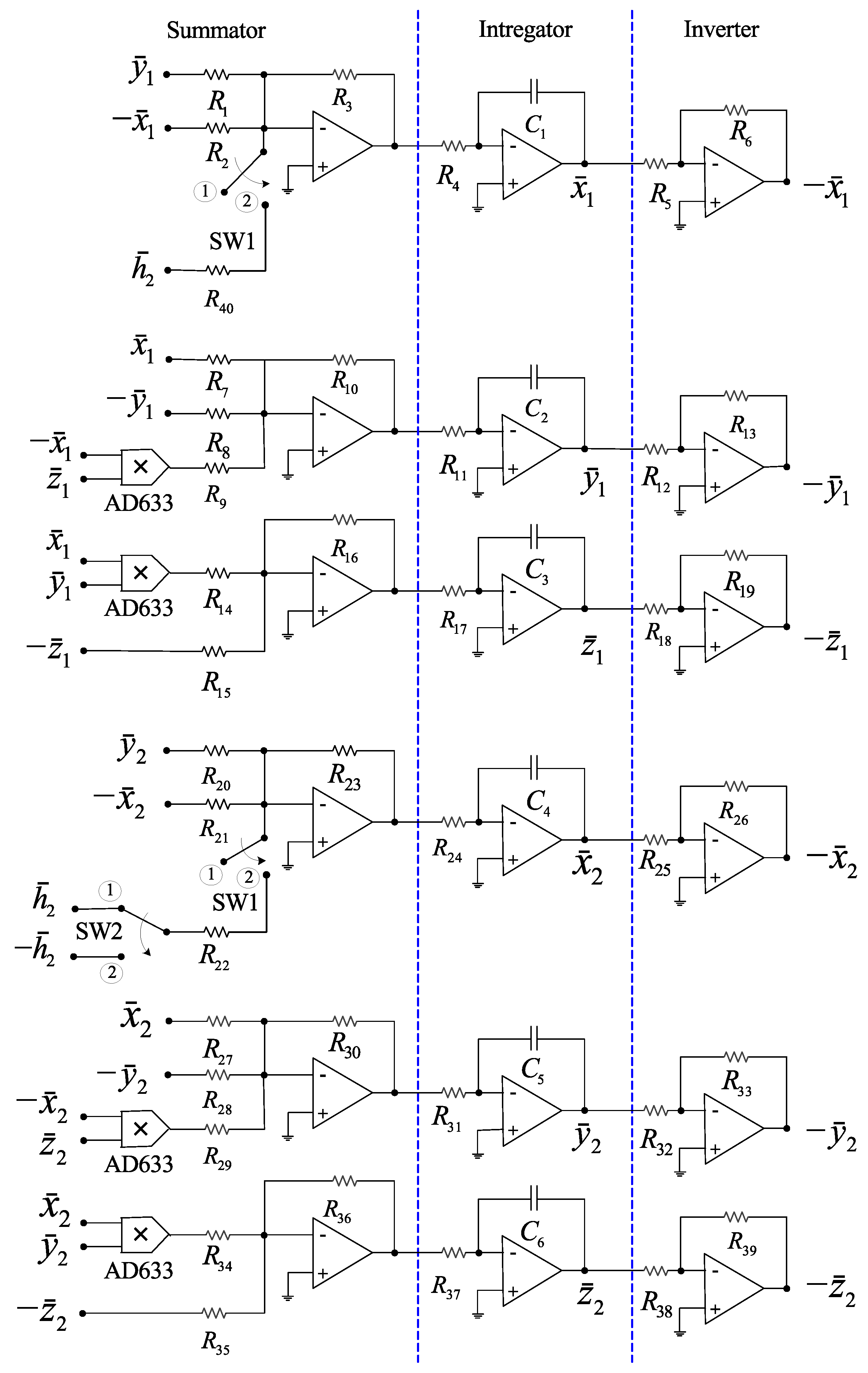
Figure 8.
Schematic diagram of the electronic circuit for implementing the Huygens’ coupling from Eq. (50)-(51).
Figure 8.
Schematic diagram of the electronic circuit for implementing the Huygens’ coupling from Eq. (50)-(51).
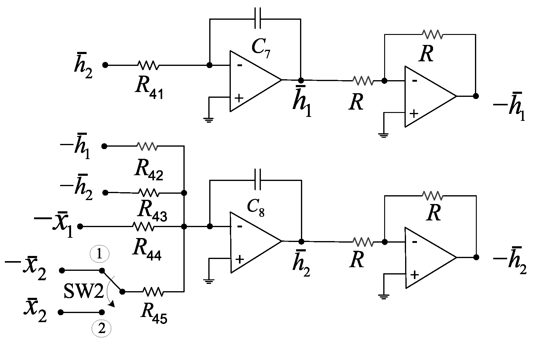
Figure 9.
Experimental results. Left: time series of the variables and . Right: phase plane for . Clearly, the variables are synchronized in anti-phase.
Figure 9.
Experimental results. Left: time series of the variables and . Right: phase plane for . Clearly, the variables are synchronized in anti-phase.
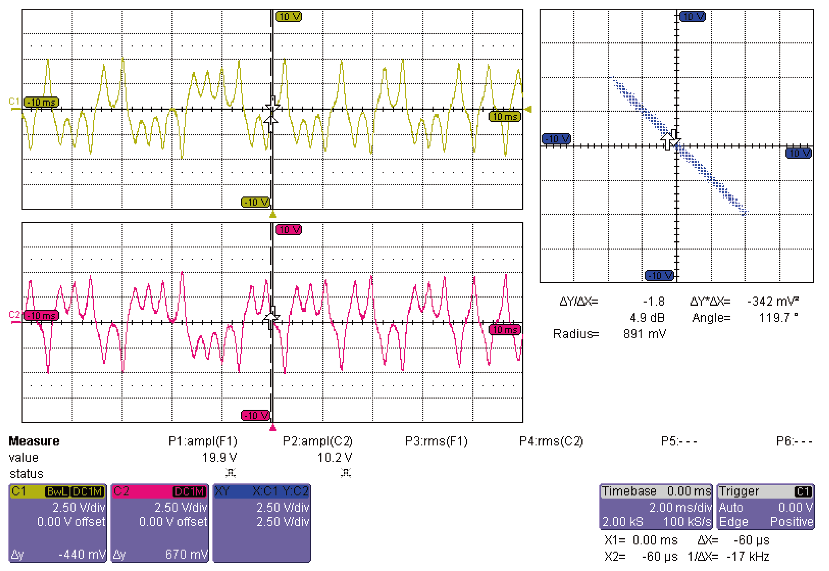
Figure 10.
Experimental results. Left: time series of the variables and . Right: phase plane for . The variables are synchronized in anti-phase.
Figure 10.
Experimental results. Left: time series of the variables and . Right: phase plane for . The variables are synchronized in anti-phase.
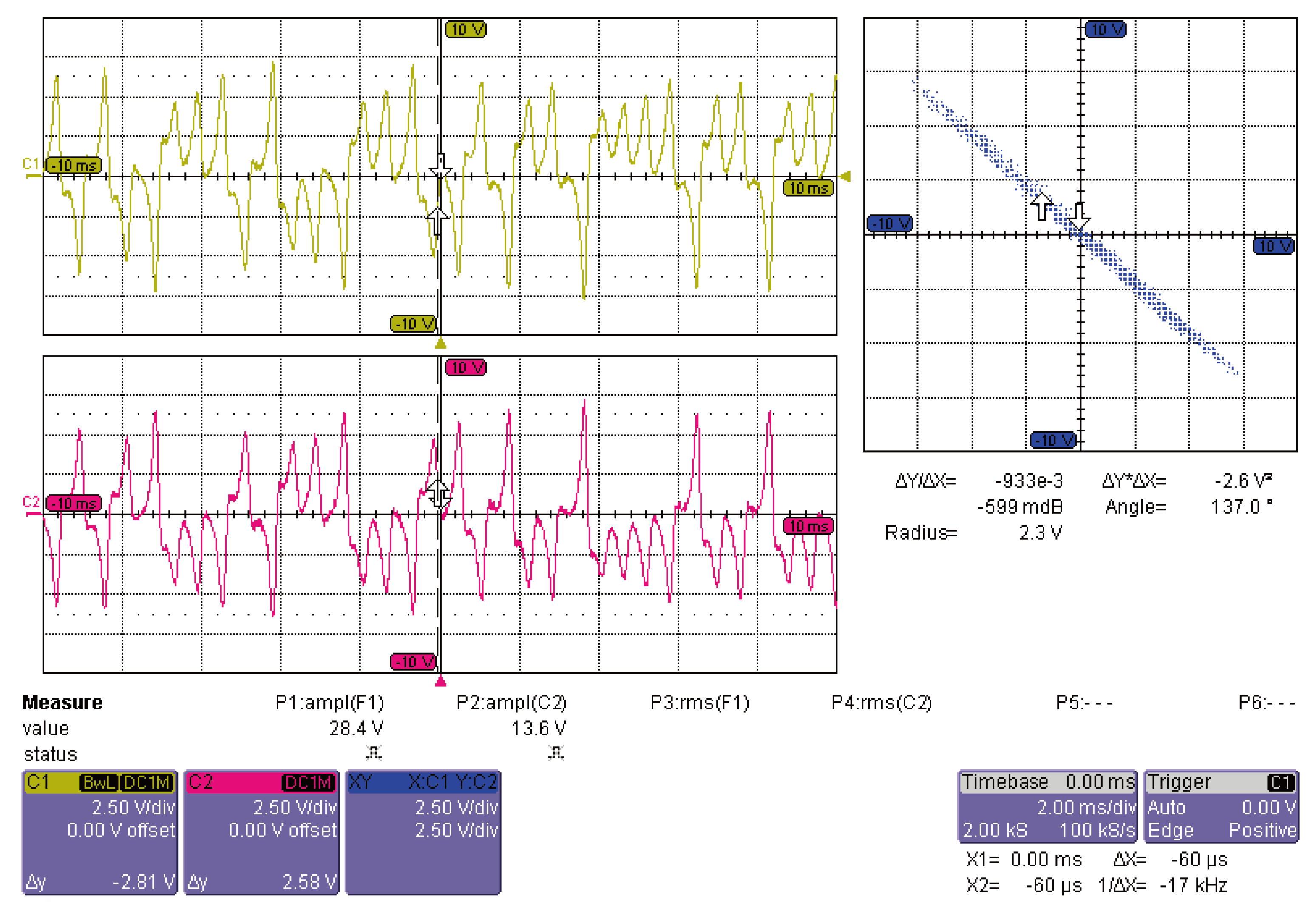
Figure 11.
Experimental results. Left: time series of the variables and . Right: phase plane for . Note that the variables achieve complete synchronization.
Figure 11.
Experimental results. Left: time series of the variables and . Right: phase plane for . Note that the variables achieve complete synchronization.
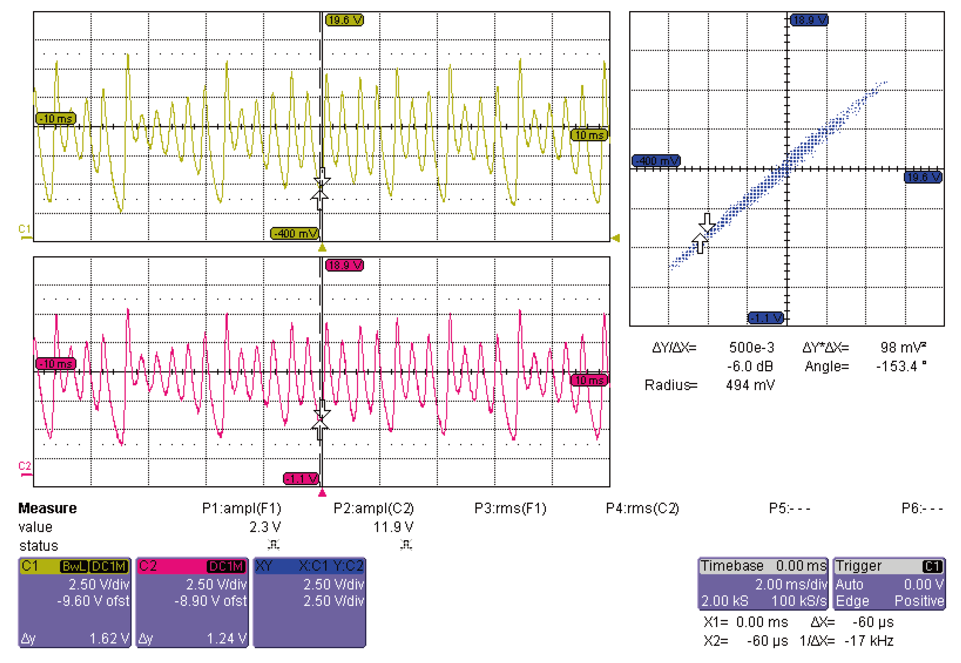

Table 1.
Parameter values of the electronic components.
| Component | Component number | Value |
|---|---|---|
| Resistances | 100k | |
| Resistances | 100k | |
| Resistances | 10k | |
| Resistances | 10k | |
| Resistances | 10k | |
| Resistances | 10k | |
| Resistances | 24k | |
| Resistances | 20k | |
| Resistances | 1M | |
| Resistances | 333k | |
| Resistance | 47k | |
| Resistance | 1000k | |
| Capacitors | 100pF | |
| Capacitors | 1000 pF | |
| Operational Amplifiers | TL084 | - |
| Multipliers | AD633 | - |
| Switch (two states) | SW1, SW2 | - |
Disclaimer/Publisher’s Note: The statements, opinions and data contained in all publications are solely those of the individual author(s) and contributor(s) and not of MDPI and/or the editor(s). MDPI and/or the editor(s) disclaim responsibility for any injury to people or property resulting from any ideas, methods, instructions or products referred to in the content. |
© 2024 by the authors. Licensee MDPI, Basel, Switzerland. This article is an open access article distributed under the terms and conditions of the Creative Commons Attribution (CC BY) license (http://creativecommons.org/licenses/by/4.0/).
Copyright: This open access article is published under a Creative Commons CC BY 4.0 license, which permit the free download, distribution, and reuse, provided that the author and preprint are cited in any reuse.


