Graph Neural Networks for Mesh Generation and Adaptation in Structural and Fluid Mechanics

Finite element discretizations of problems in computational physics often rely on hand-generated initial mesh and adaptive mesh refinement (AMR) to preferentially resolve regions containing important features during simulation. We propose Adaptnet, a Graph Neural Networks (GNNs) framework for learning mesh generation and adaptation. The model is composed of two GNNs: the first one, Meshnet, learns mesh parameters commonly used in open-source mesh generators, to generate an initial mesh from a Computer Aid Design (CAD) file; while the second one, Graphnet, learns mesh-based simulations to predict the components of an Hessian-based metric to perform anisotropic mesh adaptation. Our approach is tested on structural (Deforming plate - Linear elasticity) and fluid mechanics (Flow around cylinders - steady-state Stokes) problems. Our results show it can accurately predict the dynamics of the system and adapt the mesh accordingly. The adaptivity of the model supports learning resolution-independent dynamics and can scale to more complex state spaces at test time.

Keywords:

Subject: Computer Science and Mathematics - Computational Mathematics

1. Introduction

The generation of meshes constitutes a crucial stage in numerically simulating diverse problems within the domain of computational science [1]. Unstructured meshes find prevalent application, notably in fields like computational fluid dynamics (CFD) [2,3] and computational solid mechanics (CSM) [4,5], wherein the finite element (FE) method is employed to approximate solutions for general partial differential equations (PDE), particularly in domains featuring challenging geometries [6,7]. The accuracy of the FE solution is intricately linked to the quality of the associated mesh.

Mesh generation depends on a number of parameters, such as the local metrics at given points, but also, in the general case, the maximum and minimum sizes of cell elements, the Hausdorff coefficient, the acceptable gradation of the metric, and so on [8]. A set of parameters whose choice is far from trivial and whose poor choice can lead to meshes of poor quality, a generation process that is too long (because it is over-constrained), or even a generation failure.

A mesh can be adapted and refined to suit the physical problem being solved. The adaptation of unstructured meshes has proven very effective for stationary calculations in Fluid Mechanics and Solid Mechanics, with the aim of capturing the behaviour of physical phenomena while obtaining the desired accuracy for the numerical solution. In addition, this method considerably reduces the computational cost of the numerical solution by reducing the number of degrees of freedom. The a priori and a posteriori error estimators generally give an upper bound in the approximation error of the solved PDE. These estimates depend on the approximation space, the mesh size, the equation, the approximate solution in the case of a posteriori estimators and the exact solution in the case of a priori estimators.

Theoretical frameworks for anisotropic error estimation have been extensively developed, resulting in a degree of standardisation in the adaptation process. Various works [9,10,11], have contributed to the estimation of approximation and interpolation errors. Recent analyses of interpolation error [12,13,14,15,16] have refocused attention on metric-based mesh adaptation, particularly utilising a metric derived from a recovered Hessian. Notably, Hessian-based metric mesh adaptation offers several advantages, including a general computational framework, a relatively straightforward implementation, and, most importantly, robustness.

The use of Machine Learning (ML) or Deep Learning (DL) in the field of numerical simulation has until now focused mainly on the prediction of stationary or non-stationary fields as solutions to a given differential equation. This work has been motivated by the desire to reduce the calculation time of an approximate solution by relying on a neural network (NN) for the prediction task, rather than on a FE solver [17,18]. The field has benefited from the emergence of neural networks, and more specifically convolution neural networks (CNNs), which are generally used to extract local and global information from an image, represented as an array of pixels [19]. To reproduce this framework, the simulation domains are represented by Cartesian grids, onto which the geometry and certain initial conditions are projected [20,21,22,23,24,25]. This operation results in the loss of the information carried by the initial unstructured mesh, and produces regular meshes that can contain many more points, resulting in higher computation costs.

To address this constraint, a model can be formulated to perform convolutions on graph structures. The extension of CNNs to graphs holds significant importance, especially given that numerous solvers rely on FE methods utilising unstructured meshes for discretisation in both CFD and CSM.

Message passing neural networks (MPNNs) is a subclass of GNNs [26] that have gained prominence in the domain of mesh-based simulations, offering a framework for handling complex spatial data. The use of MPNNs in the context of mesh-based simulations represents a departure from traditional convolutional approaches, providing a more flexible methodology.

One notable instance of MPNN application is found in the work of Gilmer et al. (2017) [27], where a message-passing neural network is proposed for quantum chemistry simulations. This approach divides the convolution process into two stages: the aggregation of information from neighbouring nodes and edges into a hidden node state, followed by the use of this hidden state to update node features.

Battaglia et al. (2018) [28] introduce a slightly different approach known as graph network (GN). Messages are first transmitted from nodes to edges through an edge convolution kernel, leading to the update of edge features. Subsequently, updated edge features are aggregated to nodes using permutation-invariant operations, forming the edge messages. Finally, a node convolution kernel processes the original node features along with the edge messages to produce updated node features. This method proves to be particularly adept at capturing intricate relationships within graph-structured data.

Pfaff et al. (2021) [29] extended the application of graph networks to mesh-based simulations, focusing on scenarios such as incompressible flow around cylinders and compressible flow around airfoils. Their proposed neural network functions as an accurate incremental simulator with the added capability of adapting to the mesh structure. An intriguing feature of this approach is its ability to generalise well to mesh shapes and sizes not encountered during the training phase, emphasising its robustness in handling diverse simulation conditions.

Yet, this recent literature has not been applied to predict the complete process of AMR, from the initial geometry to the adapted mesh, in three dimensions. To this end, we propose Adaptnet, which is a framework for learning mesh parameters and tetrahedral mesh-based simulations using GNNs (Figure 1). This framework consists of two networks trained to generate unstructured meshes adapted to the physics under study:

Meshnet is trained to predict mesh parameters of a given geometry (CAD file) later used to generate an initial mesh.
Graphnet is trained to predict a metric field, either directly or indirectly by predicting the velocity field, later used to generate an anisotropic adapted mesh.

Both models are message passing graph neural networks that rely on the architecture of MeshGraphNets [29,30] that was further adapted to steady-state predictions. We will explain in detail material, methods and results for the case of the steady-state Stokes problem. The linear elasticity problem will be presented at the end to demonstrate the model’s ability to switch from one physics to another. We made use of open-source libraries to direct our work towards open-source solutions and to promote reproducibility.

The remainder of this paper is structured as follows:

Section 2: Materials and Methods - This section presents the problem statement, describes the dataset used, elaborates on the model architecture, and details the training configuration.
Section 3: Results - Here, we provide the results of our experiments, focusing on the performance of the proposed models Meshnet, Graphnet, and Adaptnet.
Section 4: Discussion - This section discusses the implications of our findings, in particular the generalization of our approach to unseen data and configurations.
Section 5: Conclusion - Finally, we summarize the key contributions of our work and suggest directions for future research.

2. Materials and Methods

2.1. Problem Statement

Both the Stokes flow and linear elasticity problems will be examined using the same geometric configuration. Specifically, each problem will be analyzed within a domain featuring a rectangular box with circular obstacles at its center, allowing for a consistent comparison of the effects of fluid flow and structural deformation on a shared geometry.

2.1.1. Stokes Problem

We consider the steady-state Stokes problem of a fluid flow around a cylinder. The domain

Ω

is a box of size

(L \times h \times 1)

with circular obstacles of radius r in the centre. The boundary

\partial Ω

is divided into four parts:

\partial Ω_{i n}

\partial Ω_{o u t}

\partial Ω_{w a l l}

and

\partial Ω_{o b s}

, corresponding to the boundaries of inlet, outlet, wall, and obstacles, respectively. The problem is defined as follows:

\{\begin{matrix} - ν Δ u + \nabla p = f & in Ω \\ \nabla \cdot u = 0 & in Ω \\ u = u_{i n} & on \partial Ω_{i n} \\ u = 0 & on \partial Ω_{o b s} \end{matrix}

(1)

where

u

is the velocity field, p is the pressure field,

f

is the body force,

ν

is the viscosity and

u_{i n}

is the inlet velocity. The inlet velocity is set to

u_{i n} = (1, 0, 0)

and the viscosity is set to

ν = 0.1

. The body force is set to

f = (0, 0, 0)

2.1.2. Linear Elasticity Problem

We consider the structural mechanics problem of an elastic plate, fixed on both sides, deformed by the action of two cylindrical actuators. The domain

Ω

is a plate of size

(L \times h \times 1)

. The boundary

\partial Ω

is divided into three parts:

\partial Ω_{l o a d}

\partial Ω_{w a l l s}

and

\partial Ω_{b o r d e r}

, corresponding to the loaded cylinders, the fixed walls and the rest of the borders of the plate . The problem is defined as follows:

\{\begin{matrix} - \nabla \cdot σ (u) = f & in Ω \\ σ (u) = λ tr (ϵ (u)) I + 2 μ ϵ (u) & in Ω \\ ϵ (u) = \frac{1}{2} (\nabla u + {(\nabla u)}^{T}) & in Ω \\ u = 0 & on \partial Ω_{w a l l s} \\ σ \cdot n = T & on \partial Ω_{l o a d} \end{matrix}

(2)

The load is set to

T = (0, - 10, 0)

, the Young modulus to

21.5 \times 10^{4} Pa

and the Poisson ratio to

0.29

. Body force is set to

f = (0, 0, 0)

2.2. Dataset

The data set is composed of 500 geometries of size

(L \times h \times 1)

with 2 circular obstacles of radius

(r_{1}, r_{2})

inside (Figure 2). The geometries are generated by randomly setting the box dimensions and the obstacles radius around control values.

The data sets are divided into 375 training samples, 75 validation samples, and 50 test samples. The training and validation samples are used to train the model, whereas the test samples are used to evaluate the model’s performance. Each sample is numbered from 0 to 499. Most illustrative figures will use sample 106 from the test set.

2.3. Mesh Parameters

CAD files are automatically generated under .geo_unrolled extension using a python script. In this work, the mesh parameters are limited to the mesh size defined at each point of the CAD file. Mesh size is set randomly around

0.1

at the circular obstacles while the one at the box extremities is set accordingly to their proximity to an obstacle, in order to test the network under real-case mesh parametrization, rather than a uniform one. Figure 3 highlights in red the 12 points representing each CAD file and labelled with a mesh size used to generate the initial mesh. Mesh generation is performed using Gmsh [31] software.

2.4. Mesh-Based Simulations

Mesh-based simulations are performed using the open-source FE library FreeFem++ [32]. For the Stokes problem, it outputs the velocity field

u

and the pressure field p on the mesh (Figure a). This library uses an Hessian-based metric to perform anisotropic mesh adaptation. Given a triangulation

Ω_{h}

, one can derive an upper bound of the approximation error using an interpolation error analysis. This upper bound is expressed thanks to the recovered Hessian of the approximated solution

u_{h}

[9]. In fact, using

P 1

linear elements, we usually cannot directly compute the Hessian of the solution. Instead, we compute an approximation called the recovered Hessian matrix

H_{R}

(

u_{h} (x)

) [10].

The recovered Hessian matrix is not a metric because it is not positive definite. Therefore, we define the following metric tensor:

M = R Λ R^{T}

(3)

where

R

is the orthogonal matrix built with the eigenvectors

(e_{1}, e_{2}, e_{3})

H_{R}

(

u_{h} (x)

) and

Λ = diag (| λ_{1} |, | λ_{2} |, | λ_{3} |)

is the diagonal matrix of absolute value of the eigenvalues of

H_{R}

(

u_{h} (x)

). By construction in FreeFem++ and Mmg[33], the prescribed size is the inverse of the square root of the metric eigenvalues, so

\frac{1}{λ_{1}^{2}}

is the size imposed in the first direction,

\frac{1}{λ_{2}^{2}}

, in the second direction, and

\frac{1}{λ_{3}^{2}}

in the third direction. Ultimately,

M

is symmetric positive definite and is characterised by only six components:

(m_{11}, m_{21}, m_{22}, m_{31}, m_{32}, m_{33})

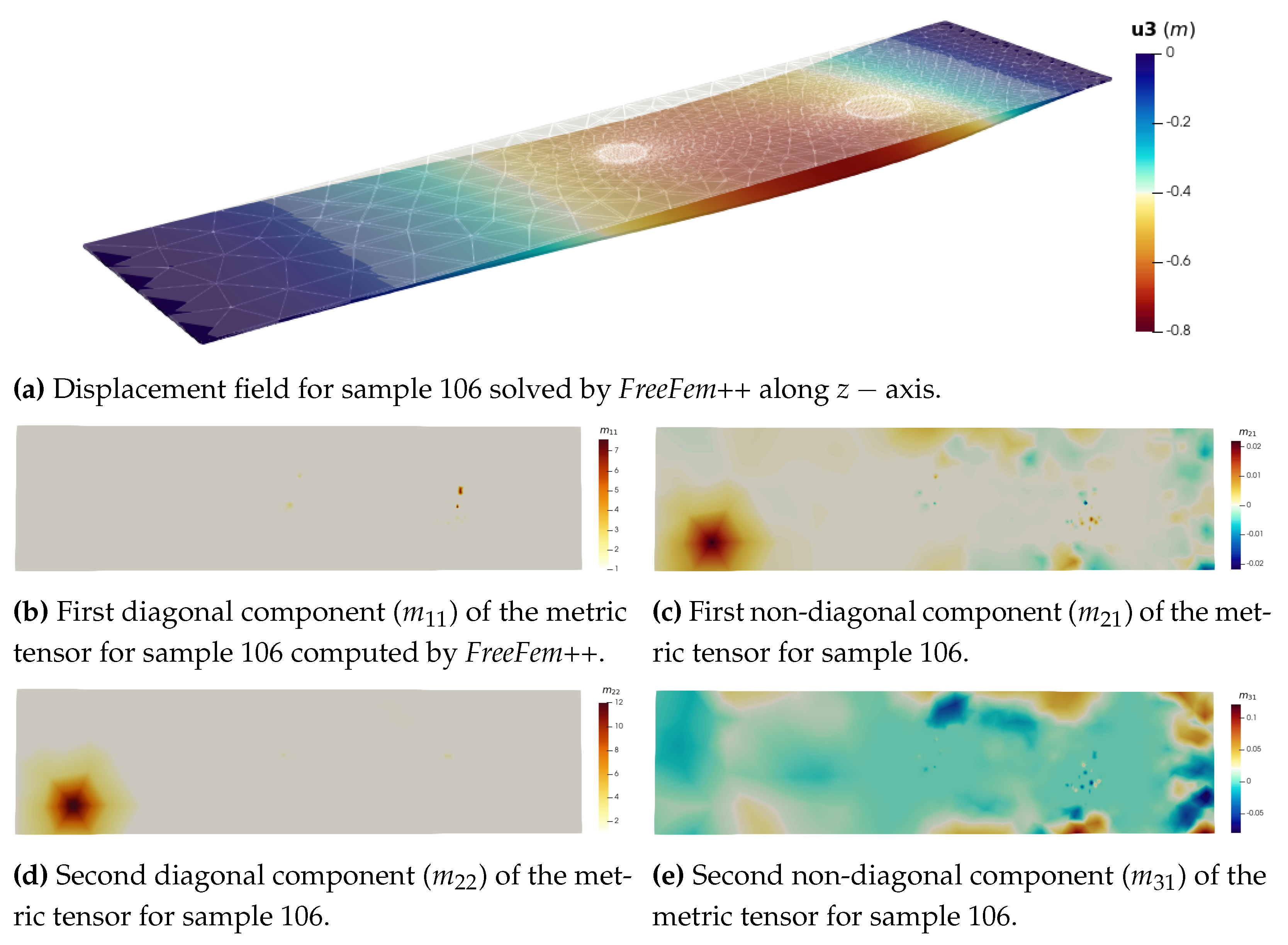
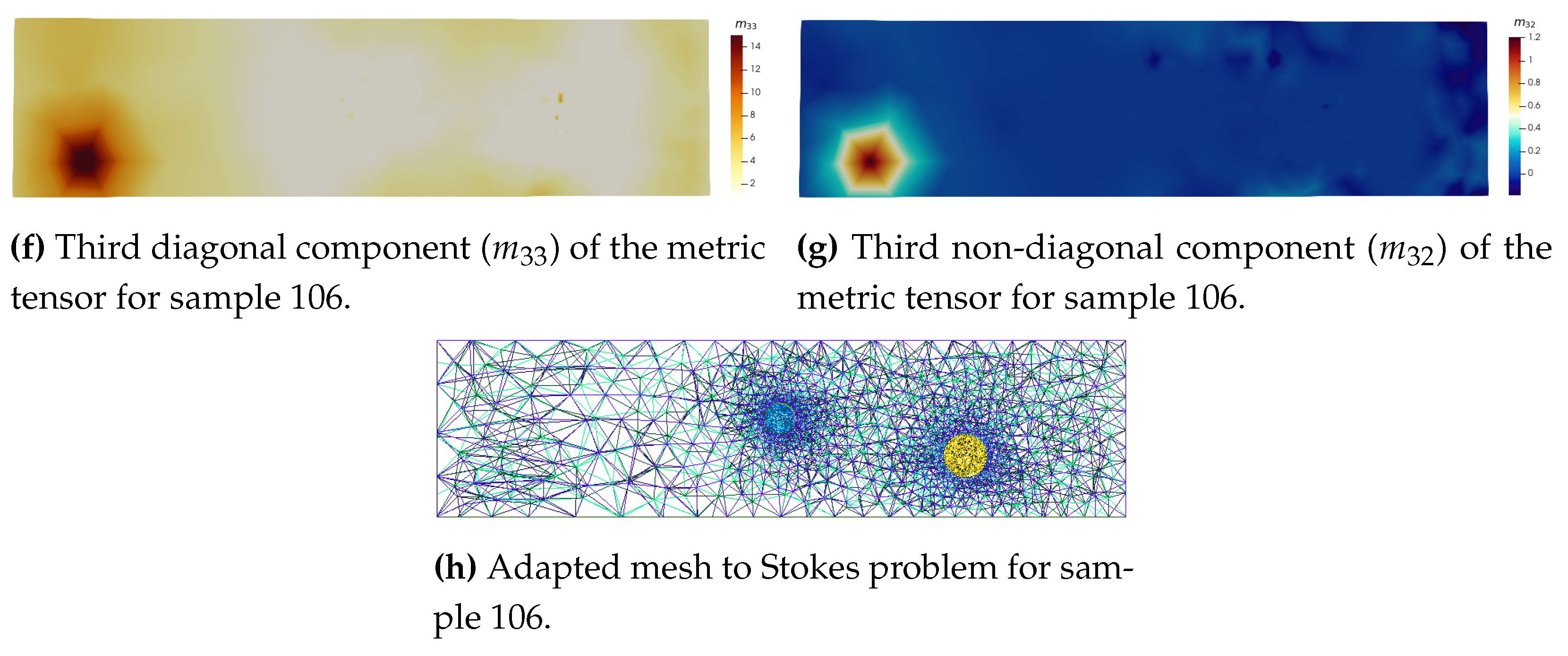
A similar set of figures can be found in Appendix A.1 for the linear elasticity problem.

2.5. Graph Representation

CAD files and unstructured meshes are essentially a list of points and edges. We can take advantage of this structure to encode these input data into graphs. Each node and edge of the graph will carry an initial information (based on coordinates, boundary conditions, and initial conditions) and the target to predict (either mesh size or physical field). For each data, we can access:

Geometry: 3D coordinates
Topology: node connections
Boundary Conditions (BC): inlet, outlet, walls, obstacles or fluid
Initial Conditions (IC): velocity and pressure field (mesh-based simulations only)

A graph is denoted by

G = (V, E)

where

V

and

E

are vertex and edge sets, respectively. Each node vertex i is represented by a graph vertex

i \in V

. Two nodes i and j connected are represented by two graph edges, with edge

(i, j) \in E

pointing to node j and edge

(j, i)

pointing to node i. In other words, the mesh nodes become graph vertices

V

, and mesh edges become bidirectional mesh-edges

E

in the graph. Properties associated with node i are termed as node feature,

x_{i}^{n} : V ⟶ R^{n_{N}}

. The properties corresponding to edge

(i, j)

are referred to as edge feature,

f (i, j) : E ⟶ R^{n_{E}}

For both networks, node features

x_{i}^{n}

consists of the belonging to a physical surface (BC)

n_{i}

, a one-hot vector of dimension 5, and, for Graphnet, the velocity field, a vector of dimension 3, such that the dimension of the node features is

n_{N}^{M e s h n e t} = 5

and

n_{N}^{G r a p h n e t} = 8

. The edge feature

f (i, j)

of edge

(i, j)

is constructed to enrich the graph connectivity information with the (signed) distance between nodes,

u_{j} - u_{i} \in R^{3}

, and its absolute value, such that

n_{E} = 4

. Figure 5 and Figure 6 illustrate this process for Meshnet and Graphnet, respectively.

2.6. Model

In both Meshnet and Graphnet, the behaviour of the targeted variables are captured by learning directly on the graph using latent node and edge features derived from the physical node and edge features reviewed in Section 2.5. We use a graph neural network model with an Encoder-Processer-Decoder architecture [29,34]. See Appendix A.2 for more details.

The architecture proposed by Pfaff et al. [29] is essentially designed to predict the dynamical states of a system over time. Since our test cases are steady-state predictions, we adapt this architecture following the work of Harsch et al. [35] to better capture local and global features.

2.6.1. Encoder

Using the graph representation of Section 2.5, we compute the initial latent feature vectors,

v_{i}^{0} \in R^{n_{H}}

and

e_{(i, j)}^{0} \in R^{n_{H}}

from the physical feature vectors,

x_{n}^{i}

and

f (i, j)

. The hyperparameter

n_{H}

denotes the size of the latent vectors. The computation of the latent vectors is done using the node and edge multilayer perceptrons (MLPs) (Table A1), denoted respectively by

{mlp}_{v}^{0}

and

{mlp}_{e}^{0}

, as follows:

\{\begin{matrix} v_{i}^{0} = {mlp}_{v}^{0} (x_{n}^{i}) \\ e_{(i, j)}^{0} = {mlp}_{e}^{0} (f (i, j)) \end{matrix}

(4)

2.6.2. Processor

The processor consists of m message-passing steps computed in sequence. At step

l \in {1, \dots, m}

in the sequence, each graph edge feature

e_{(i, j)}^{l}

is updated using its value at the previous message-passing step

l - 1

and the values of the adjacent node features at step

l - 1

, as follows

e_{(i, j)}^{l} = {mlp}_{e}^{l} ([e_{(i, j)}^{l - 1}, v_{i}^{l - 1}, v_{j}^{l - 1}]), l \in {1, \dots, m}

(5)

to obtain the updated value. In Equation (5), the operator

[\cdot]

concatenates the given arguments on the feature dimension. Then, each graph node

v_{i}^{l}

is updated using its value at the previous message-passing step,

l - 1

, and the aggregation of its incident edge features at step

l - 1

v_{i}^{l} = {mlp}_{v}^{l} ([v_{i}^{l - 1}, \sum_{j \in adj (i)} e_{(i, j)}^{l}]), l \in {1, \dots, m}

(6)

where

adj (i)

is the set of nodes connected to node i. Using Equations (5) and (6), the processor computes an updated set of node features.

The update of the edge-based messages,

e_{(i, j)}^{l}

, is the key to the accuracy of the flow predictions as it propagates information between neighbouring graph nodes (i.e., between neighbouring mesh cell elements). This design choice differentiates MeshGraphNets [29] from other classical GNN frameworks relying only on node features, such as GCN and GraphSAGE [36].

2.6.3. Decoder

After performing m steps of the previously described process, the decoder maps the updated graph nodes latent features

v_{i}^{l}

to the node-based properties in physical state using MLP as follows:

{\hat{y}}_{i} = {mlp}^{m + 1} (v_{i}^{l})

(7)

where m is the number of steps performed by the processor.

2.6.4. Local and Global Features

To increase the ability to extract local and global properties, we adopt the structure proposed by Wang et al. [37] for Dynamic Graph CNN and adapted by Harsch et al. [35]. This adaptation aggregates the information given by each message passing block to calculate a global feature vector. In that sense, the number of layers is reduced to 5, instead of 15 previously. To avoid potential overfitting, a pooling operation is added, and the result is concatenated with the previous local features. This adapted version is called Graphnet (Pool) (Figure 8).

2.7. Loss Function and Optimiser

We train both networks by minimising the error between the true node label and the predicted node label. We use the per-node root mean square error (RMSE) loss to quantify the data error for each simulation. The loss function reads:

L = \sqrt{\frac{1}{n_{B}} \sum_{i = 1}^{n_{B}} {∥ y_{i} - {\hat{y}}_{i} ∥}_{2}^{2}}

(8)

where

n_{B}

denotes the number of nodes in a batch of training meshes,

y_{i}

denotes the true output in the data set,

{\hat{y}}_{i}

is the output predicted by the network, as formalised in Equation (7).

ADAM optimiser is used and the learning rate is constant, equal to

0.001

. With the data set and a fixed set of hyper-parameters at hand, each epoch takes

30 s

on two NVIDIA A100 GPUs. The value of specific training hyperparameters is given in Table A3.

3. Results

3.1. Meshnet

3.1.1. Fine Tuning Input Data for Message-Passing GNN

Meshnet was trained to learn to predict the mesh size at each point of a given geometry. These mesh sizes are then used to generate a first mesh using Gmsh [31]. The loss curve highlights the message-passing nature of this GNN. However, when we first trained the network, the case did not converge, giving the blue cyan loss curve on Figure 9a. During the graph-encoding step (Figure 5), we pass to the network the distance of each edge of the geometry in the edge feature matrix. However, in our geometrical representation, the points of the box are not linked to the obstacles (Figure 9b). Thus, the network is blind and cannot learn this specific mapping. As a workaround, we manually added controlled edges so that the new edge feature will keep the distance between the points of the box and the obstacles (Figure 9b).

3.1.2. Evaluating Meshes Similarity and Quality

To evaluate the network, we are also interested in the mesh similarities between the mesh generated with the ground truth parameters, and the one generated by the predictions. The comparison of the number of points and tetrahedra between the ground truth and the prediction can only give us a small overview (Figure 10a).

We can take, for instance, the cases of simulations 106 and 130. The former shows a good similarity in terms of points and tetrahedra, while the latter has a prediction with twice as many points and tetrahedra than the ground truth. To better assess the quality of each mesh, we use "Glassmaier" parameter [38] defined as

Q_{G} = 1 + \frac{True Surf .}{Ideal Surf .} + \frac{True Vol .}{Ideal Vol .}

(9)

and takes on values between 1 and 3. It tends to describe the dimensionality of the figure, as listed in Table 1. The ideal volume and surface are calculated for a regular tetrahedron with a side length equal to the average of the 6 distances between the 4 points.

The distribution of this quality estimator among the ground truth and predicted meshes are very similar for both cases (Figure 10b), and the visual observation confirm this conclusion (Figure 11). In fact, the number of points and tetrahedra is greatly sensitive to the the mesh size defined on the obstacles, since it is the smallest one, thus giving the greatest number of points of tetrahedra. Thus, in the case of simulation 130, the ground truth and the prediction have a similar pattern of mesh, but one is finer at the obstacles.

3.2. Graphnet

3.2.1. Direct Predictions: Velocity and Anisotropic Metric Fields

Graphnet was trained to learn mesh-based simulations. First, we trained one network to predict the three components of the velocity field, in order to use it to compute an anisotropic metric from the Hessian of the velocity field (Figure 12a). Then, we decided to predict directly the metric field by training one network for each of the six components of the metric tensor(Figure 12b). Finally, we use the adapted architecture Graphnet (Section 2.6.4) to improve the training (Figure 12c).

The case of simulation 106 highlights that the velocity field, in addition to be a 3-component field, is a more complex learning task than the metric field. As expected, error is concentrated around the obstacles, where the gradients are higher and the boundary conditions changing (Figure 13). The metric field prediction still shows some error, but catches precisely the evolution of this variable across the simulation domain (Figure 14).

3.2.2. Mesh Adaptation

Ultimately, we are looking for the resulting adapted mesh generated through this metric field. We use Mmg software [33] to realise such adaptation in 3D. Again, generated meshes show great visual similarity (Figure 15), confirmed by quality analysis (Figure 16b). As expected, the number of points and tetrahedra has been divided by two through the AMR process, both for ground truth and prediction in the case of simulation 106.

This result can be extended to the remaining simulations of the test sets. The relative errors in number of points and tetrahedra (Figure 16a) show great improvement in comparison to Meshnet (Figure 10a), meaning that the gap in points an tetrahedra created by the prediction of the initial mesh has very little influence on the ultimate adapted mesh. Mesh quality is more important, as it is almost conserved through the AMR process (Figure 16b).

3.3. Adaptnet

Adaptnet is the framework combining Meshnet and Graphnet (Figure 1. Given an initial geometry, it will predict initial mesh sizes (Meshnet) to produce an initial mesh and predict on this mesh an metric field to adapt it to the Stokes problem. This process has already been illustrated through the example of the 3-hole geometry. First, we showed how Meshnet produces an initial mesh (Figure 17), and then, we use this mesh to predict the anisotropic metric tensor at each point of the simulation domain and adapt the mesh (Figure 18). By predicting directly the metric tensor, we are able to skip the calculation of the velocity field, unlike a FE solver, speeding up calculation time accordingly (Table 3). For Graphnet, we compare the prediction time of the six models (one for each component of the metric tensor) with the computation time of FreeFem++, on the 3-hole test case, using a single CPU. For Meshnet, the prediction time should be compared with the engineering time needed to choose the mesh parameters.

4. Discussion

4.1. Meshnet Generalisation

The architectural choice of using relative encoding on graphs has been shown to be very conducive to generalisation [34]. Our model generalises well, as can be seen when we want it to predict the mesh size at each point on a 3-hole geometry (Figure 17).

4.2. Graphnet Generalisation

The same observation can be made when we want to predict the adaptation metric in a 3-hole geometry (Figure 18).

Finally, we tested our model with a different geometry from those seen previously. This time, we chose a square (Figure 20). The point here is not to test our model with every possible shape but simply to highlight its ability to interpolate in a wide spectrum of graph structures.

4.3. Linear Elasticity Problem

The attempt to train the graph neural network (GNN) on the linear elasticity problem proved to be less successful than expected (Figure 22), highlighting the challenges inherent in this complex task. Despite meticulous parameter tuning and a comprehensive dataset, the network struggled to effectively capture and generalise the underlying patterns within the graph structures. The intricate interplay of nodes and edges posed a formidable challenge, and the model exhibited difficulties in discerning meaningful relationships and dependencies.

These results underscore the need for further investigation into refining GNN architectures and training methodologies, emphasising the intricate nature of graph-based data and the nuances associated with their representation in neural networks.

At first glance, the quality of the mesh produced may seem even better than the reference (Figure 23). But quantitative analysis highlights the poorer quality of prediction in this case (Figure 24). Still, it can be noticed that the plate is very thin along z - axis. As a consequence, the tetrahedra generated will necessarily be stretched in this direction, resulting in lower quality. But the overall quality distribution is more satisfactory, as the first visual impression suggested.

5. Conclusions

We propose a Graph Neural Network mesh-based method to model fluid dynamics and solid mechanics problems for an accurate and efficient prediction of anisotropic adaptation metric fields. We extended the approach of Pfaff et al. [29] to tetrahedral meshes in three dimensions. Following the work of Harsch et al. [35], we adapted the GNN architecture to better suit the prediction of steady states. Our method may allow for more efficient simulations than traditional simulators, and because it is differentiable, it could be used to retrieve the Hessian matrix directly, when traditional solvers have to compute a recovered Hessian matrix.

The experiments demonstrate the model’s strong understanding of the geometric structure. The method is independent of the structure of the simulation domain, being able to capture highly irregular meshes. We show that the model does not require any a priori domain information, e.g. inflow velocity or material parameters. Thus, the model can be used for any other systems represented as field data.

Training phase underlined the model’s strong understanding of the geometric structure of the unstructured meshes. It was shown that it can achieve effective prediction with the sole knowledge of connectivity and the belonging to a physical surface. It doesn’t rely on any prior information such as the inflow velocity or the material parameters. This, it can be easily adapted and scaled to other physical problems governed by PDEs. However, our test show that some specific tuning might be necessary to achieve correct predictions when adapting from a fluid problem to a solid one for instance.

The strength of this work lies in the tetrahedral mesh generation and adaptation pipeline. The emphasis was placed on producing work based on open source tools [31,32,33] to promote reproducibility and enable others to build on it. Future work in this area should address several topics. It could explore more complex geometries to prove its applicability to industrial problems. Alternative architectures could also be explored. Adding concatenation and pooling has been shown to improve performance, but other options could show even better improvements. Finally, this framework could be further improved by adding a specific physical constraints to the loss function, similar to Physics-Informed Neural Networks (PINNs) [39], which could enable learning on sparse datasets, reducing the need for generating hundreds of simulations.

Author Contributions

Conceptualization, Mesri Y. and Parret-Fréaud A.; methodology, Pelissier U. and Mesri Y.; software, Pelissier U.; validation, Mesri Y. and Parret-Fréaud A. and Bordeu F.; formal analysis, Pelissier U.; investigation, Pelissier U.; resources, Mesri Y. and Parret-Fréaud A. and Bordeu F.; data curation, Pelissier U.; writing—original draft preparation, Pelissier U.; writing—review and editing, Pelissier U. and Mesri Y. and Parret-Fréaud A. and Bordeu F.; visualization, Pelissier U.; supervision, Mesri Y. and Parret-Fréaud A. and Bordeu F.; project administration, Mesri Y. and Parret-Fréaud A.; funding acquisition, Mesri Y. and Parret-Fréaud A. All authors have read and agreed to the published version of the manuscript.

Funding

This research received no external funding.

Data Availability Statement

Data is publicly available at https://github.com/UgoPelissier/adaptnet.

Acknowledgments

This work has been supported by SafranTech.

Conflicts of Interest

The authors declare no conflict of interest.

Abbreviations

The following abbreviations are used in this manuscript:

AMR	Adaptive Mesh Refinement
ADAM	Adaptive Moment Estimation
BC	Boundary Conditions
CAD	Computer Aid Design
CFD	Computational Fluid Dynamics
CSM	Computational Solid Mechanics
CNN	Convolutional neural network
DL	Deep Learning
FE	Finite Element
GN	Graph Network
IC	Initial Conditions
ML	Machine Learning
NN	Neural Network
PINN	Physics-Informed Neural Networks
RMSE	Root Mean Square Error

Appendix A.

Appendix A.1. Linear elasticity problem

Figure A1. Finite Element solving of Elasticity problem and anisotropic metric computation for sample 106.

Appendix A.2. Model

The MLPs of the Encoder, Processor, and Decoder are ReLUactivated two-hidden-layer MLPs with layer and output size of 128, except for the Decoder MLP whose output size matches the prediction. All MLPs outputs except the Decoder one are normalized by a LayerNorm. All input and target features are normalised to zero mean unit variance, using dataset statistics.

Table A1. Details of node and edge encoders.

Node MLP ( ${mlp}_{v})$	Edge MLP ( ${mlp}_{e})$
Input: x	Input: x
$x = Linear (5 / 8, 128) (x)$	$x = Linear (3, 128) (x)$
$x = RELU (x)$	$x = RELU (x)$
$x = Linear (128, 128) (x)$	$x = Linear (128, 128) (x)$
$x = RELU (x)$	$x = RELU (x)$
$x = Linear (128, 128) (x)$	$x = Linear (128, 128) (x)$
$x = RELU (x)$	$x = RELU (x)$
$x = Linear (128, 128) (x)$	$x = Linear (128, 128) (x)$
$x = LayerNorm (128) (x)$	$x = LayerNorm (128) (x)$

Table A2. Hyperparameters used for processor.

Parameter name	Value
Number of GNN layer for the processor	15
Latent size for the processor	128
Activation	ReLu
Type of normalization	Layer normalization
Input feature size of Node MLP	256
Input feature size of Edge MLP	384

References

Zhang, Z.; Wang, Y.; Jimack, P.K.; Wang, H. MeshingNet: A New Mesh Generation Method based on Deep Learning, 2020, [arXiv:math.NA/2004.07016]. arXiv:math.NA/2004.07016].
Economon, T.D.; Palacios, F.; Copeland, S.R.; Lukaczyk, T.W.; Alonso, J.J. SU2: An Open-Source Suite for Multiphysics Simulation and Design. AIAA Journal 2016, 54, 828–846. [Google Scholar] [CrossRef]
Ramamurti, R.; Sandberg, W. Simulation of Flow About Flapping Airfoils Using Finite Element Incompressible Flow Solver. AIAA Journal 2001, 39, 253–260. [Google Scholar] [CrossRef]
Panthi, S.; Ramakrishnan, N.; Pathak, K.; Chouhan, J. An analysis of springback in sheet metal bending using finite element method (FEM). Journal of Materials Processing Technology 2007, 186, 120–124. [Google Scholar] [CrossRef]
Yazid, A.; Abdelkader, N.; Abdelmadjid, H. A state-of-the-art review of the X-FEM for computational fracture mechanics. Applied Mathematical Modelling 2009, 33, 4269–4282. [Google Scholar] [CrossRef]
Shewchuk, J. Delaunay refinement algorithms for triangular mesh generation. Computational Geometry 2002, 22, 21–74. [Google Scholar] [CrossRef]
Si, H.; Sadrehaghighi, I. Tetgen -A Delaunay-Based Quality Tetrahedral Mesh Generator. ACM Transactions on Mathematical Software 2022. [Google Scholar] [CrossRef]
Lei, N.; Li, Z.; Xu, Z.; Li, Y.; Gu, X. What’s the Situation with Intelligent Mesh Generation: A Survey and Perspectives, 2023, [arXiv:cs.AI/2211.06009].
Almeida, R.C.; Feijóo, R.A.; Galeao, A.C.; Padra, C.; Silva, R.S. Adaptive finite element computational fluid dynamics using an anisotropic error estimator. Computer Methods in Applied Mechanics and Engineering 2000, 182, 379–400. [Google Scholar] [CrossRef]
Mesri, Y.; Zerguine, W.; Digonnet, H.; Silva, L.; Coupez, T. , Dynamic Parallel Adaption for Three Dimensional Unstructured Meshes: Application to Interface Tracking; 2008; pp. 195–212. [CrossRef]
Mesri, Y.; Khalloufi, M.; Hachem, E. On optimal simplicial 3D meshes for minimizing the Hessian-based errors. Applied Numerical Mathematics 2016, 109, 235–249. [Google Scholar] [CrossRef]
Loseille, A.; Alauzet, F. Continuous mesh framework part I: well-posed continuous interpolation error. SIAM Journal on Numerical Analysis 2011, 49, 38–60. [Google Scholar] [CrossRef]
Agouzal, A.; Vassilevski, Y.V. Minimization of gradient errors of piecewise linear interpolation on simplicial meshes. Computer methods in applied mechanics and engineering 2010, 199, 2195–2203. [Google Scholar] [CrossRef]
Labbé, P.; Dompierre, J.; Vallet, M.G.; Guibault, F. Verification of three-dimensional anisotropic adaptive processes. International journal for numerical methods in engineering 2011, 88, 350–369. [Google Scholar] [CrossRef]
Mesri, Y.; Guillard, H.; Coupez, T. Automatic coarsening of three dimensional anisotropic unstructured meshes for multigrid applications. Applied Mathematics and Computation 2012, 218, 10500–10519. [Google Scholar] [CrossRef]
Kamenski, L.; Huang, W. How a nonconvergent recovered Hessian works in mesh adaptation. SIAM Journal on Numerical Analysis 2014, 52, 1692–1708. [Google Scholar] [CrossRef]
Ladický, L.; Jeong, S.; Solenthaler, B.; Pollefeys, M.; Gross, M. Data-driven fluid simulations using regression forests. 2015; 34. [Google Scholar] [CrossRef]
Wiewel, S.; Becher, M.; Thuerey, N. Latent-space Physics: Towards Learning the Temporal Evolution of Fluid Flow, 2019, [arXiv:cs.LG/1802.10123].
Lecun, Y.; Bengio, Y. Convolutional Networks for Images, Speech, and Time-Series. 1995.
Guo, X.; Li, W.; Iorio, F. Convolutional Neural Networks for Steady Flow Approximation. Proceedings of the 22nd ACM SIGKDD International Conference on Knowledge Discovery and Data Mining; Association for Computing Machinery: New York, NY, USA, 2016. [Google Scholar] [CrossRef]
Zhu, Y.; Zabaras, N. Bayesian deep convolutional encoder–decoder networks for surrogate modeling and uncertainty quantification. Journal of Computational Physics 2018, 366, 415–447. [Google Scholar] [CrossRef]
Jin, X.; Cheng, P.; Chen, W.L.; Li, H. Prediction model of velocity field around circular cylinder over various Reynolds numbers by fusion convolutional neural networks based on pressure on the cylinder. Physics of Fluids 2018, 30. [Google Scholar] [CrossRef]
Lee, S.; You, D. Data-driven prediction of unsteady flow over a circular cylinder using deep learning. Journal of Fluid Mechanics 2019, 879, 217–254. [Google Scholar] [CrossRef]
Thuerey, N.; Weißenow, K.; Prantl, L.; Hu, X. Deep Learning Methods for Reynolds-Averaged Navier–Stokes Simulations of Airfoil Flows. AIAA Journal 2020, 58, 25–36. [Google Scholar] [CrossRef]
Patil, A.; Viquerat, J.; Larcher, A.; El Haber, G.; Hachem, E. Robust deep learning for emulating turbulent viscosities. Physics of Fluids 2021, 33. [Google Scholar] [CrossRef]
Scarselli, F.; Gori, M.; Tsoi, A.C.; Hagenbuchner, M.; Monfardini, G. The Graph Neural Network Model. IEEE Transactions on Neural Networks 2009, 20, 61–80. [Google Scholar] [CrossRef]
Gilmer, J.; Schoenholz, S.S.; Riley, P.F.; Vinyals, O.; Dahl, G.E. Neural Message Passing for Quantum Chemistry, 2017, [arXiv:cs.LG/1704.01212]. arXiv:cs.LG/1704.01212].
Battaglia, P.W.; Hamrick, J.B.; Bapst, V.; Sanchez-Gonzalez, A.; Zambaldi, V.; Malinowski, M.; Tacchetti, A.; Raposo, D.; Santoro, A.; Faulkner, R.; Gulcehre, C.; Song, F.; Ballard, A.; Gilmer, J.; Dahl, G.; Vaswani, A.; Allen, K.; Nash, C.; Langston, V.; Dyer, C.; Heess, N.; Wierstra, D.; Kohli, P.; Botvinick, M.; Vinyals, O.; Li, Y.; Pascanu, R. Relational inductive biases, deep learning, and graph networks, 2018, [arXiv:cs.LG/1806.01261]. arXiv:cs.LG/1806.01261].
Pfaff, T.; Fortunato, M.; Sanchez-Gonzalez, A.; Battaglia, P.W. Learning Mesh-Based Simulation with Graph Networks. International Conference on Learning Representations, 2021.
Ju, X.; Hamon, F.P.; Wen, G.; Kanfar, R.; Araya-Polo, M.; Tchelepi, H.A. Learning CO₂ plume migration in faulted reservoirs with Graph Neural Networks, 2023, [arXiv:cs.LG/2306.09648]. arXiv:cs.LG/2306.09648].
Geuzaine, C.; Remacle, J.F. Gmsh: A 3-D finite element mesh generator with built-in pre- and post-processing facilities. International Journal for Numerical Methods in Engineering 2009, 79, 1309–1331. [Google Scholar] [CrossRef]
Hecht, F. New development in FreeFem++. J. Numer. Math. 2012, 20, 251–265. [Google Scholar] [CrossRef]
Dobrzynski, C. MMG3D: User Guide. Technical Report RT-0422, INRIA, 2012.
Sanchez-Gonzalez, A.; Godwin, J.; Pfaff, T.; Ying, R.; Leskovec, J.; Battaglia, P.W. Learning to Simulate Complex Physics with Graph Networks, 2020, [arXiv:cs.LG/2002.09405]. arXiv:cs.LG/2002.09405].
Harsch, L.; Riedelbauch, S. Direct Prediction of Steady-State Flow Fields in Meshed Domain with Graph Networks, 2021, [arXiv:physics.flu-dyn/2105.02575]. arXiv:physics.flu-dyn/2105.02575].
Zhou, J.; Cui, G.; Hu, S.; Zhang, Z.; Yang, C.; Liu, Z.; Wang, L.; Li, C.; Sun, M. Graph Neural Networks: A Review of Methods and Applications, 2021, [arXiv:cs.LG/1812.08434]. A: Neural Networks; arXiv:cs.LG/1812.08434].
Wang, Y.; Sun, Y.; Liu, Z.; Sarma, S.E.; Bronstein, M.M.; Solomon, J.M. Dynamic Graph CNN for Learning on Point Clouds, 2019, [arXiv:cs.CV/1801.07829]. arXiv:cs.CV/1801.07829].
vom Stein, R.; Glassmeier, K.H.; Dunlop, M. A Configuration Parameter for the Cluster Satellites., 1992.
Raissi, M.; Perdikaris, P.; Karniadakis, G.E. Physics-informed neural networks: A deep learning framework for solving forward and inverse problems involving nonlinear partial differential equations. Journal of Computational Physics 2019, 378, 686–707. [Google Scholar] [CrossRef]

Figure 1. Diagram of Adaptnet framework to predict a mesh adapted to some physics, given an initial geometry.

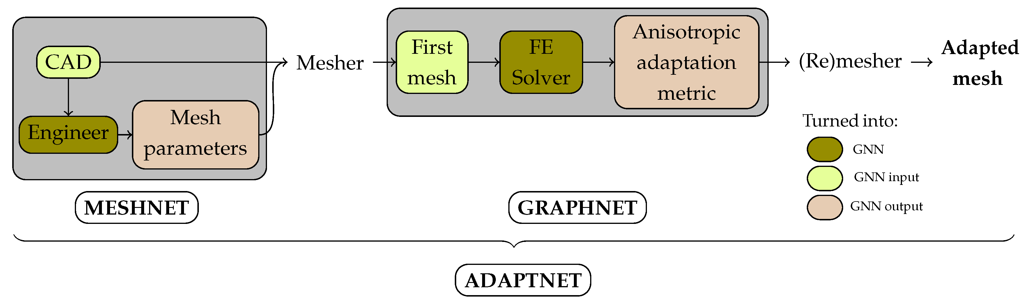
Figure 2. Labelled CAD from fluid and structural mechanics cases.

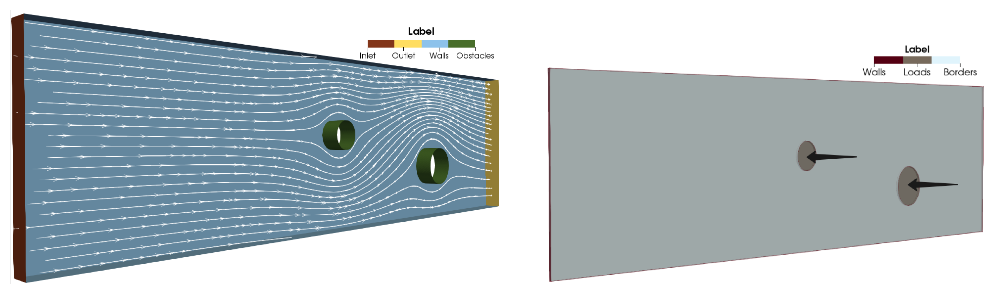
Figure 3. Generated 3D tetrahedral mesh for sample 106 using mesh size at geometry points highlighted in red. The mesh is generated using Gmsh [31].

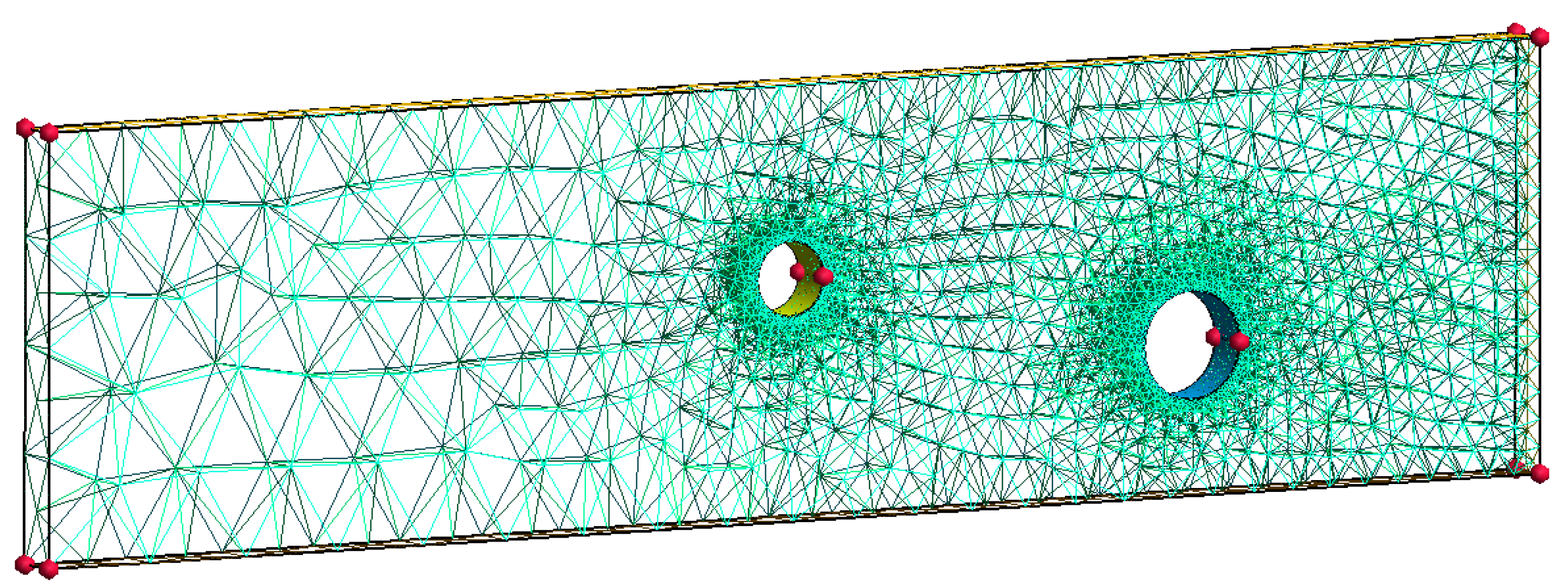
Figure 4. Finite Element solving of Stokes problem and anisotropic metric computation.

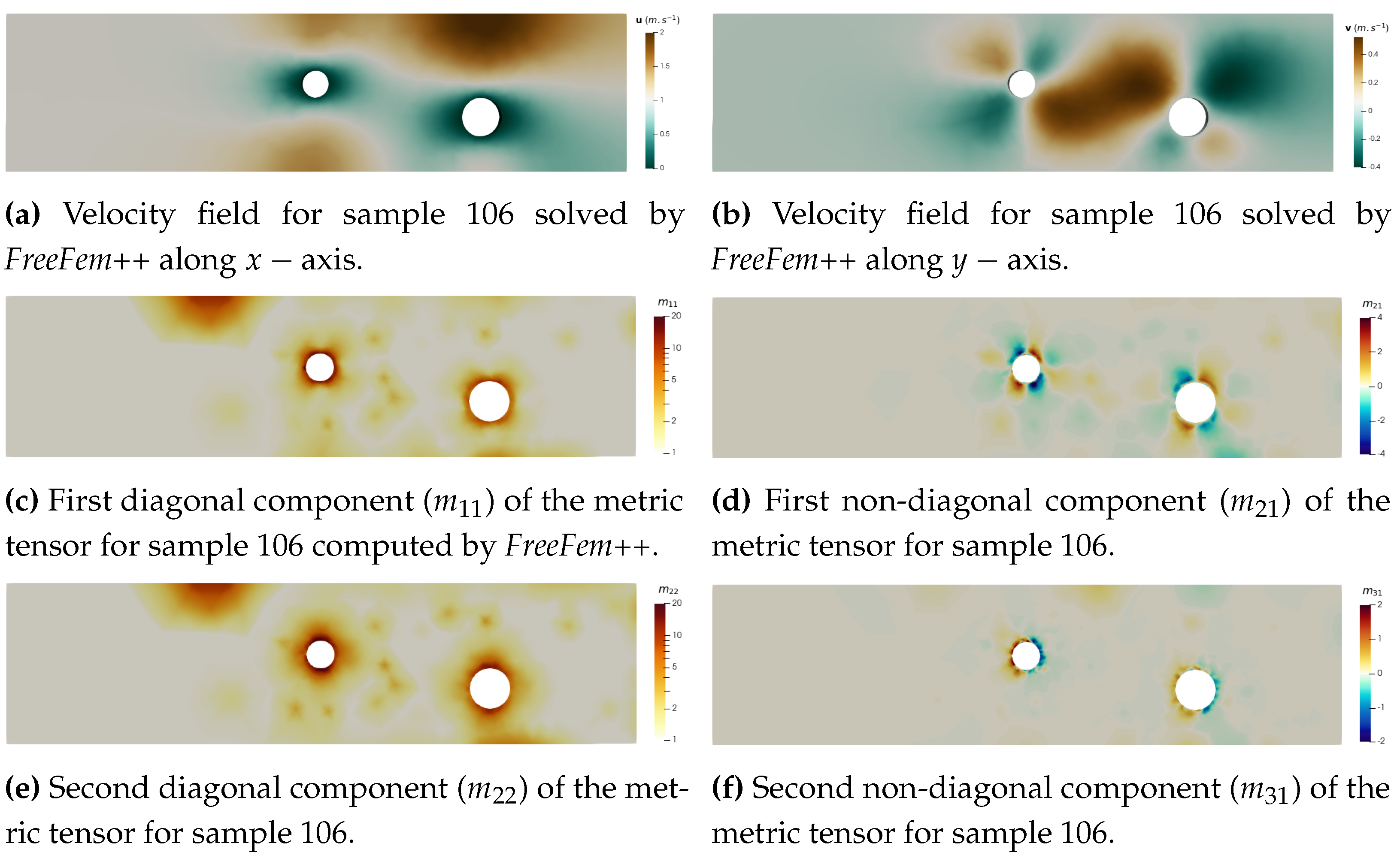
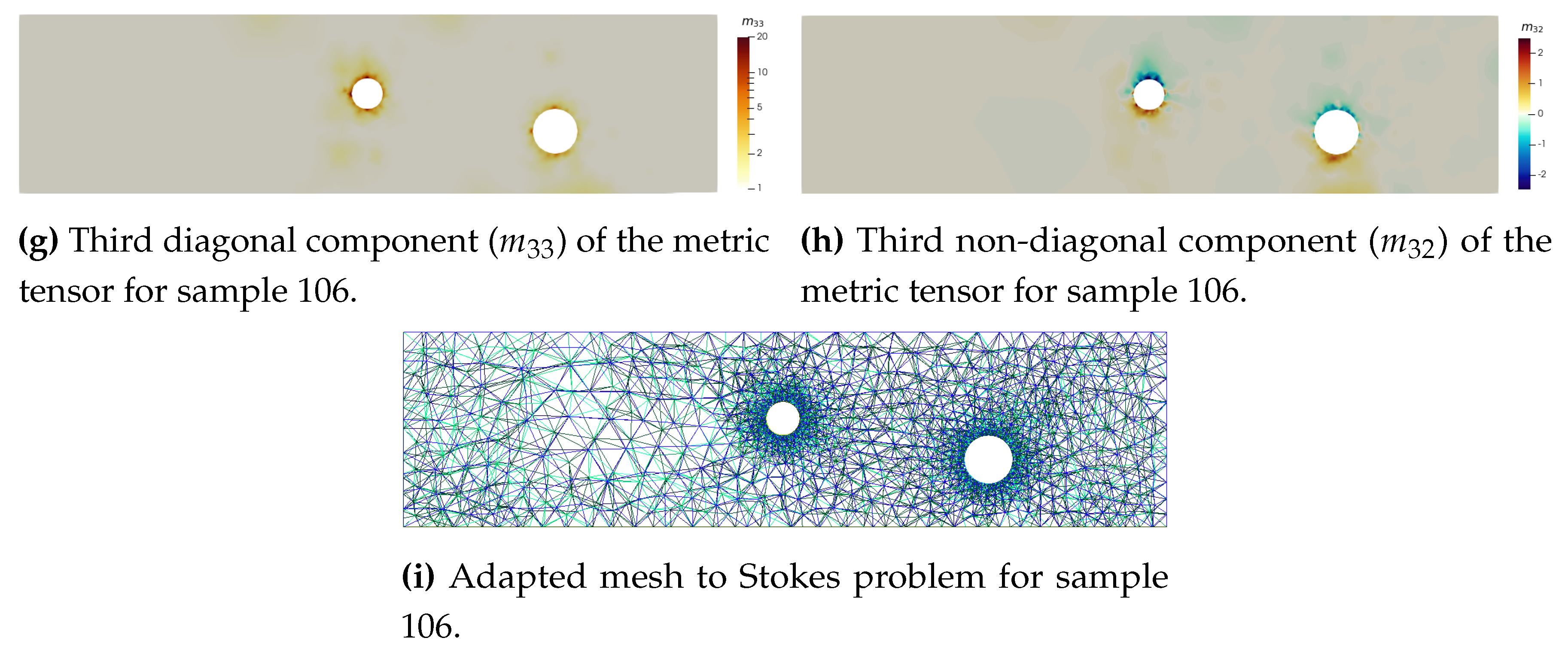
Figure 5. Meshnet encoding illustration. The encoder encodes the current mesh into a graph

G = (V, E)

. Mesh nodes become graph vertices

V

, and mesh edges become bidirectional mesh-edges in the graph

E

Figure 5. Meshnet encoding illustration. The encoder encodes the current mesh into a graph

G = (V, E)

. Mesh nodes become graph vertices

V

, and mesh edges become bidirectional mesh-edges in the graph

E

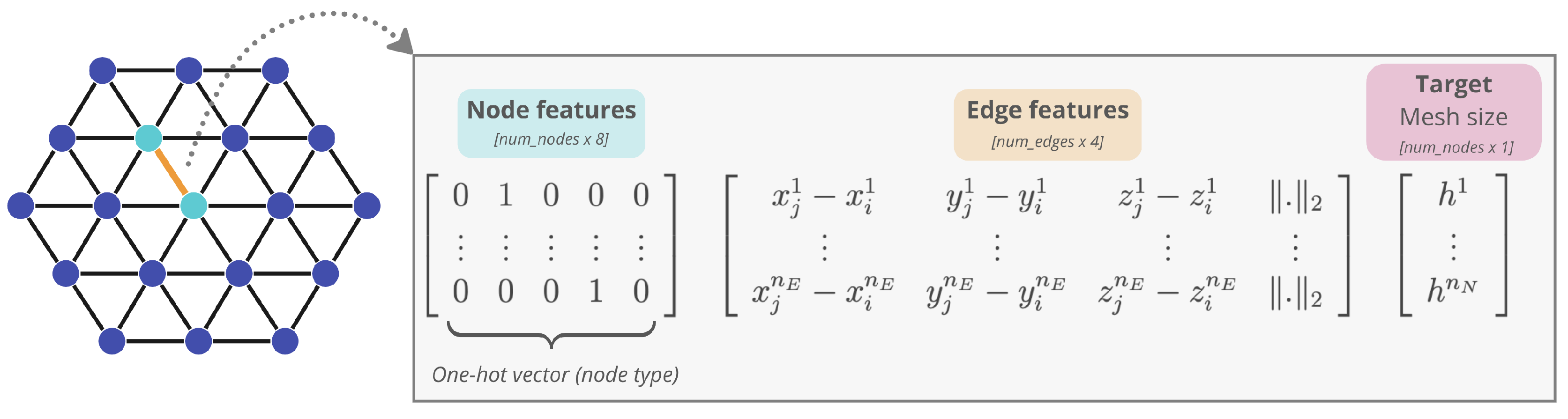
Figure 6. Graphnet encoding illustration.

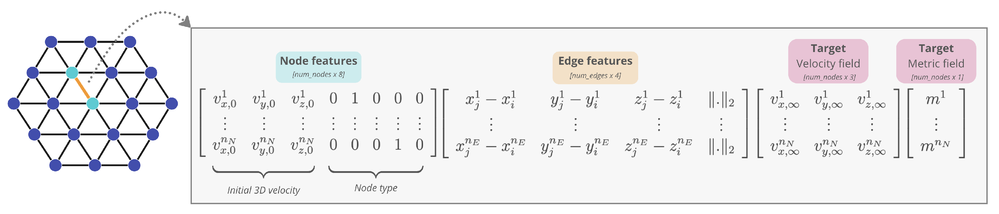
Figure 7. Diagram of Graphnet operating on Stokes problem. The model uses an Encoder-Processer-Decoder architecture. The encoder transforms the input mesh into a graph. The processor performs several rounds of message passing along mesh edges, updating all node and edge embeddings. The decoder returns the velocity or metric field for each node, which is then used to compute the Hessian and the metric field in order to trigger remeshing.

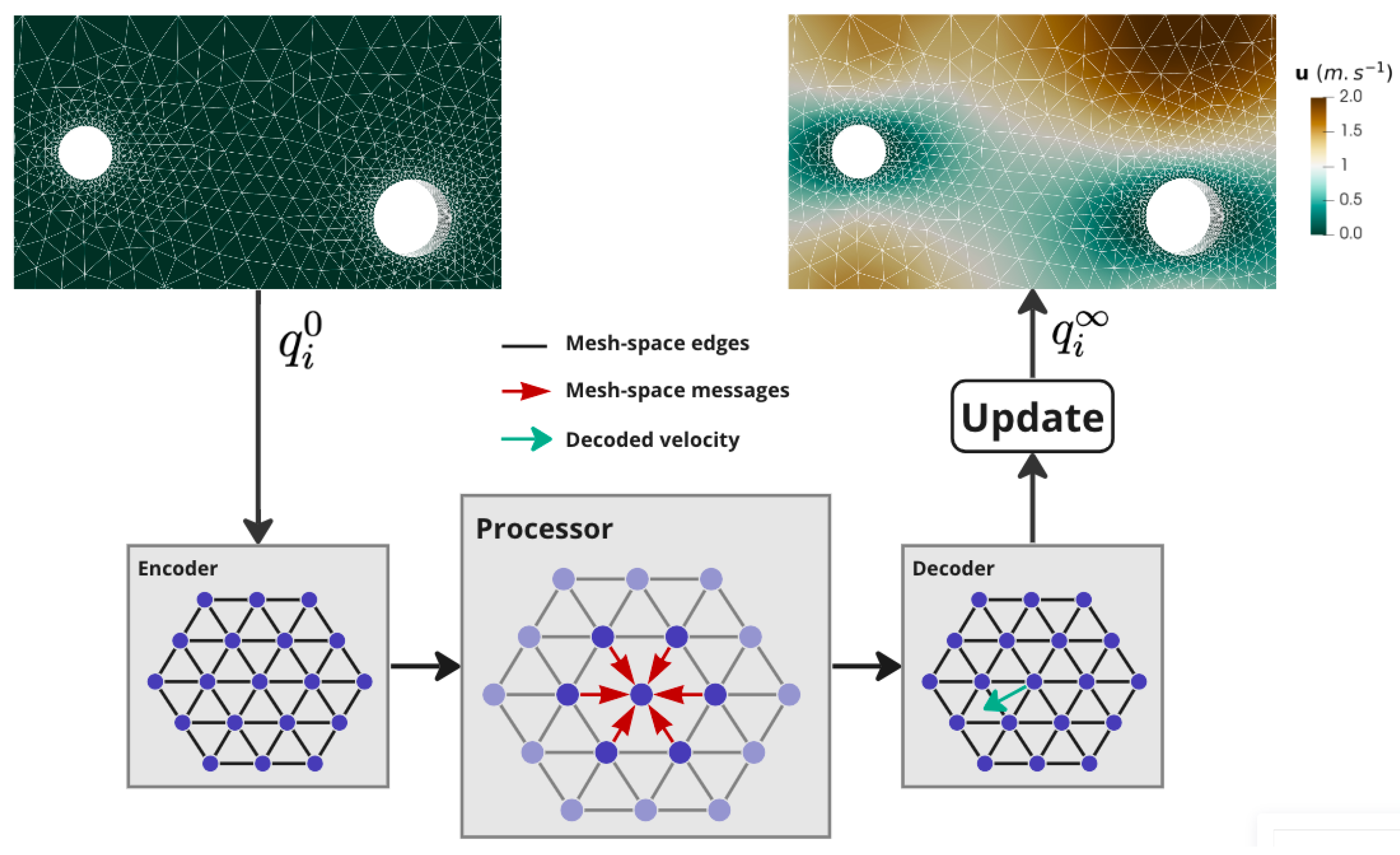
Figure 8. Adapted model architecture using message passing block with local and global descriptor [35] (operator ⊕ denotes the concatenation).

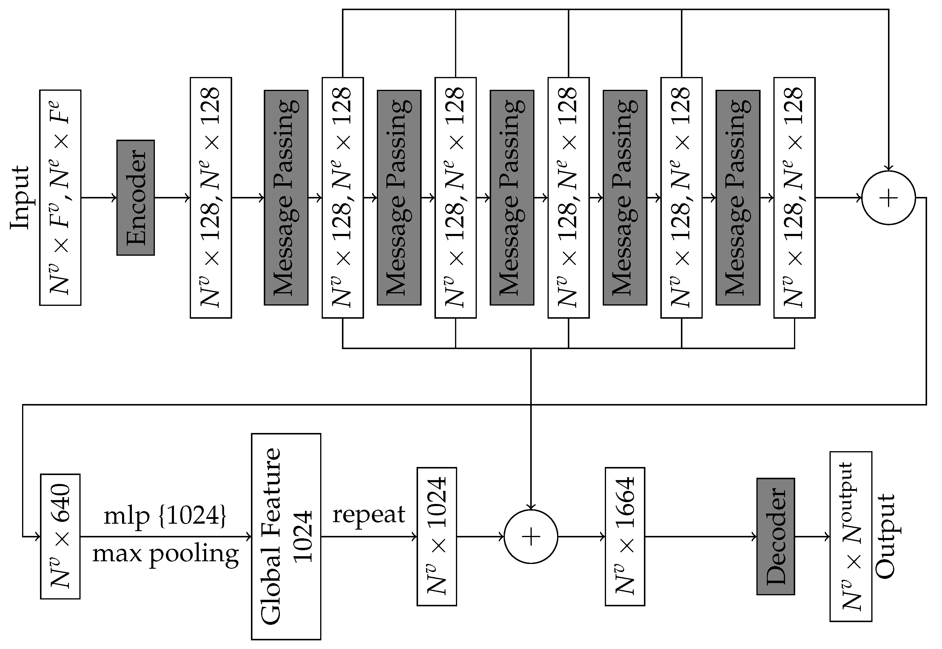
Figure 9. Influence of the controlled edges on Meshnet learning curve through message-passing.

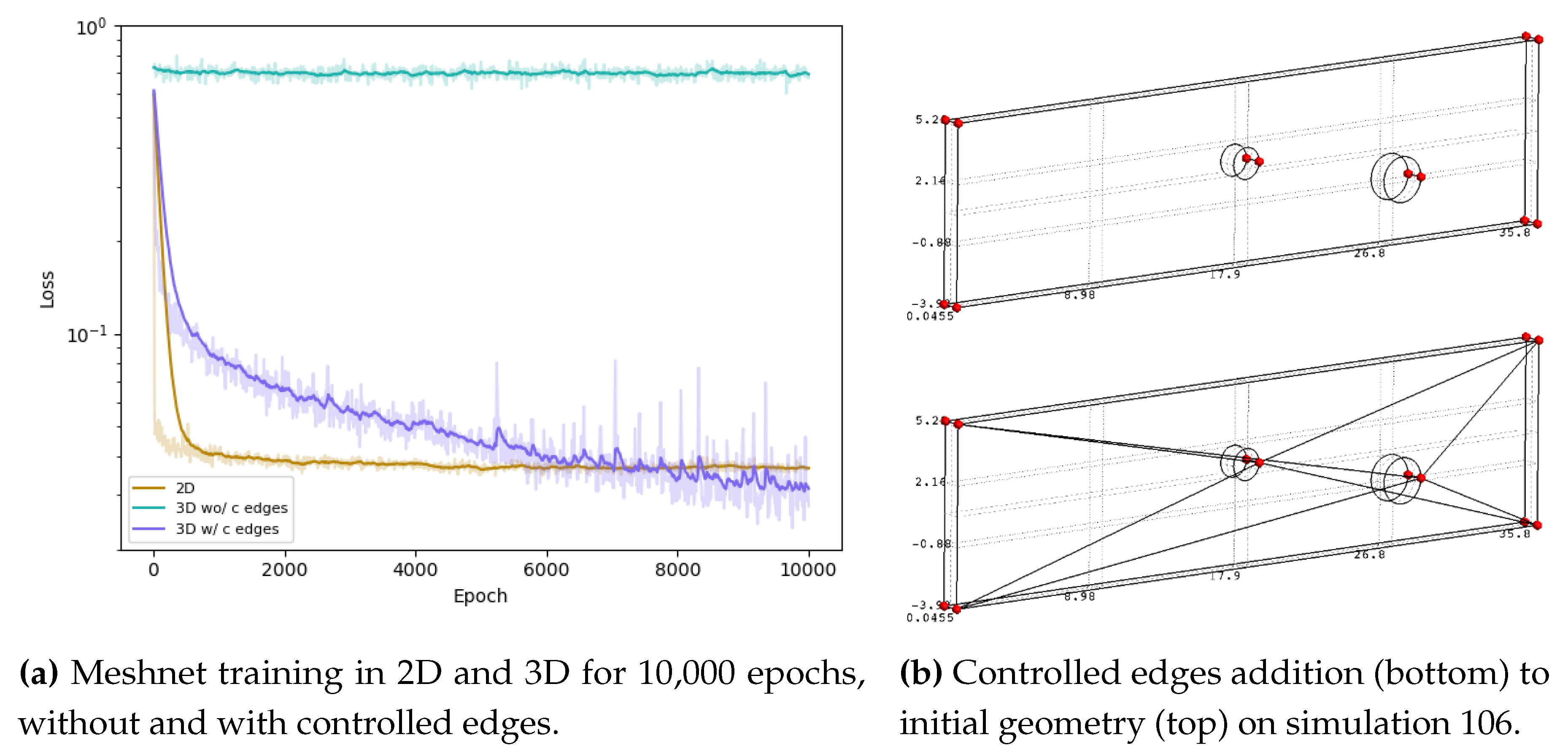
Figure 10. Quality of meshes predicted by Meshnet on simulations from the test set.

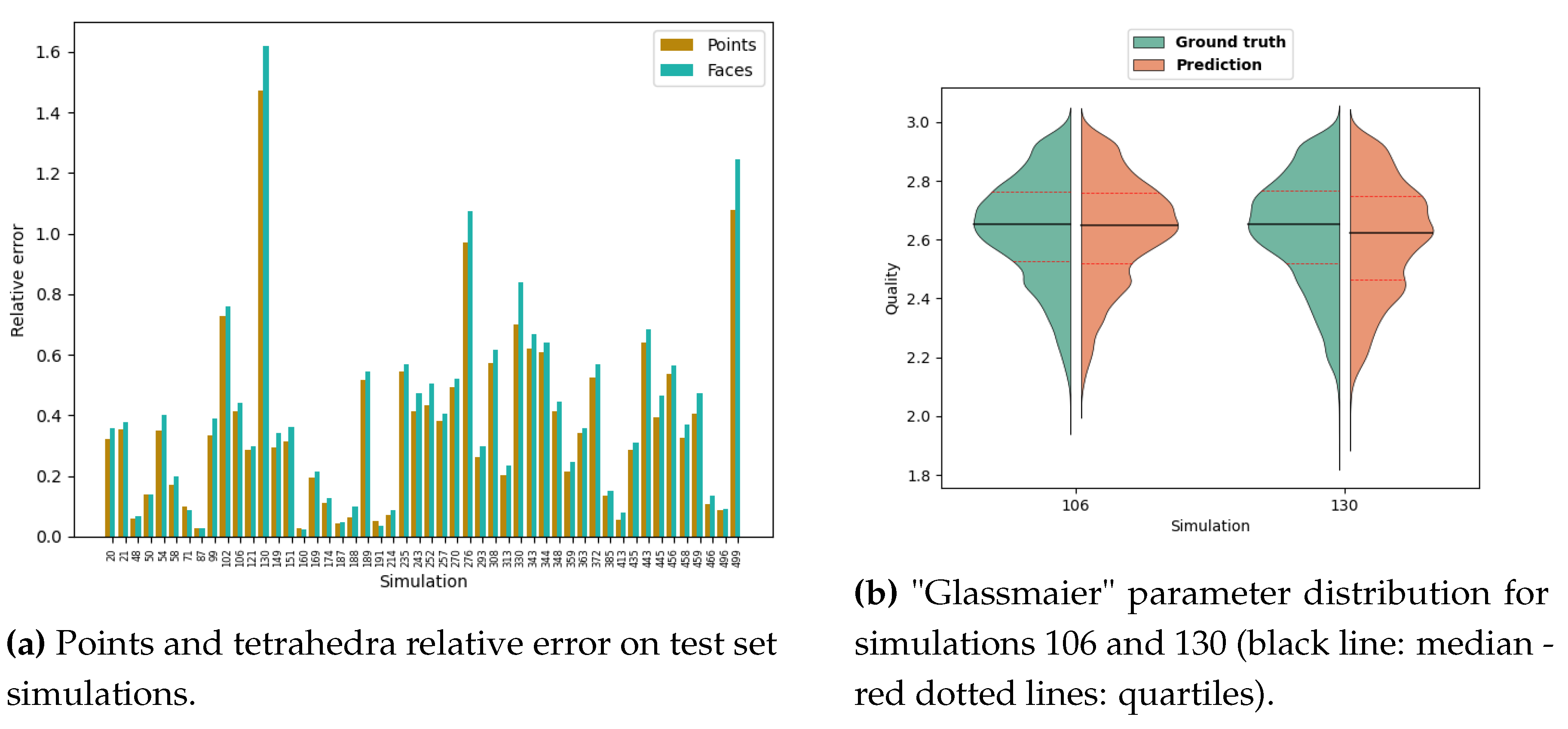
Figure 11. Mesh visualisation of simulations 106 and 130 using Gmsh [31].

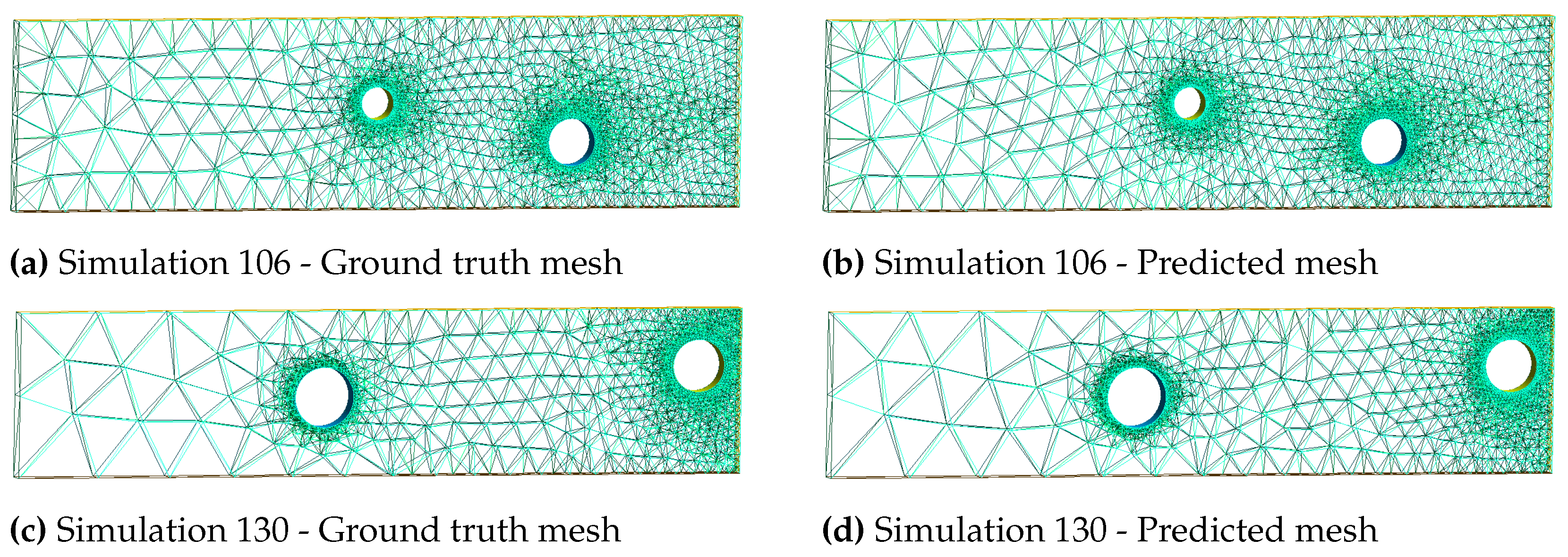
Figure 12. Graphnet training for 10,000 epochs.

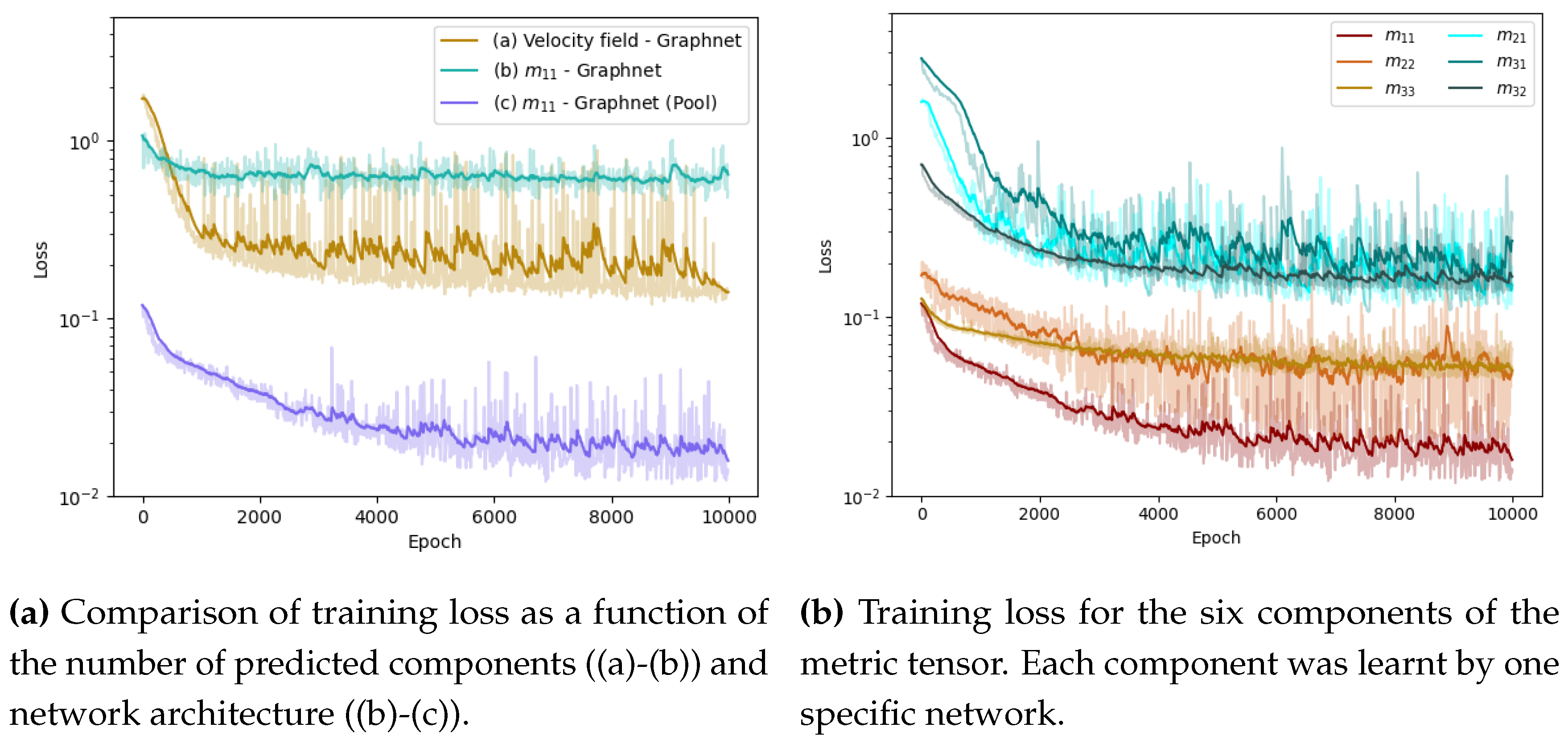
Figure 13. Graphnet training for 10,000 epochs.

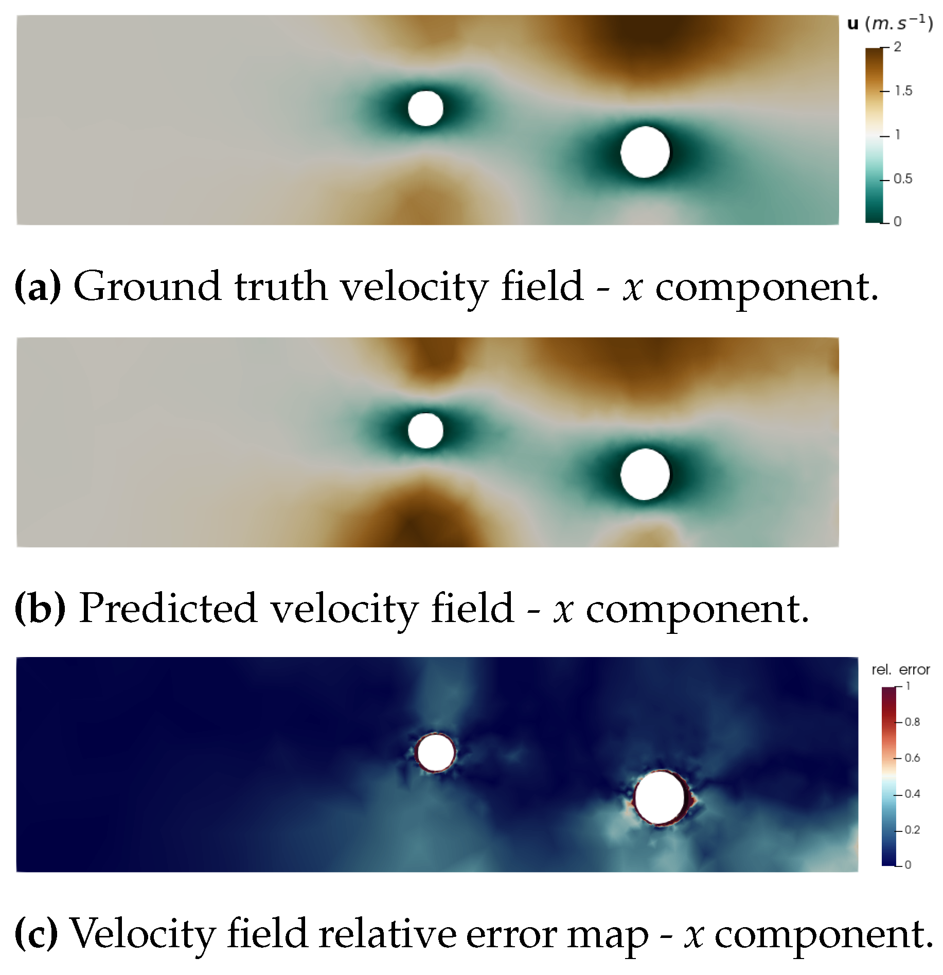
Figure 14. Graphnet training for 10,000 epochs.

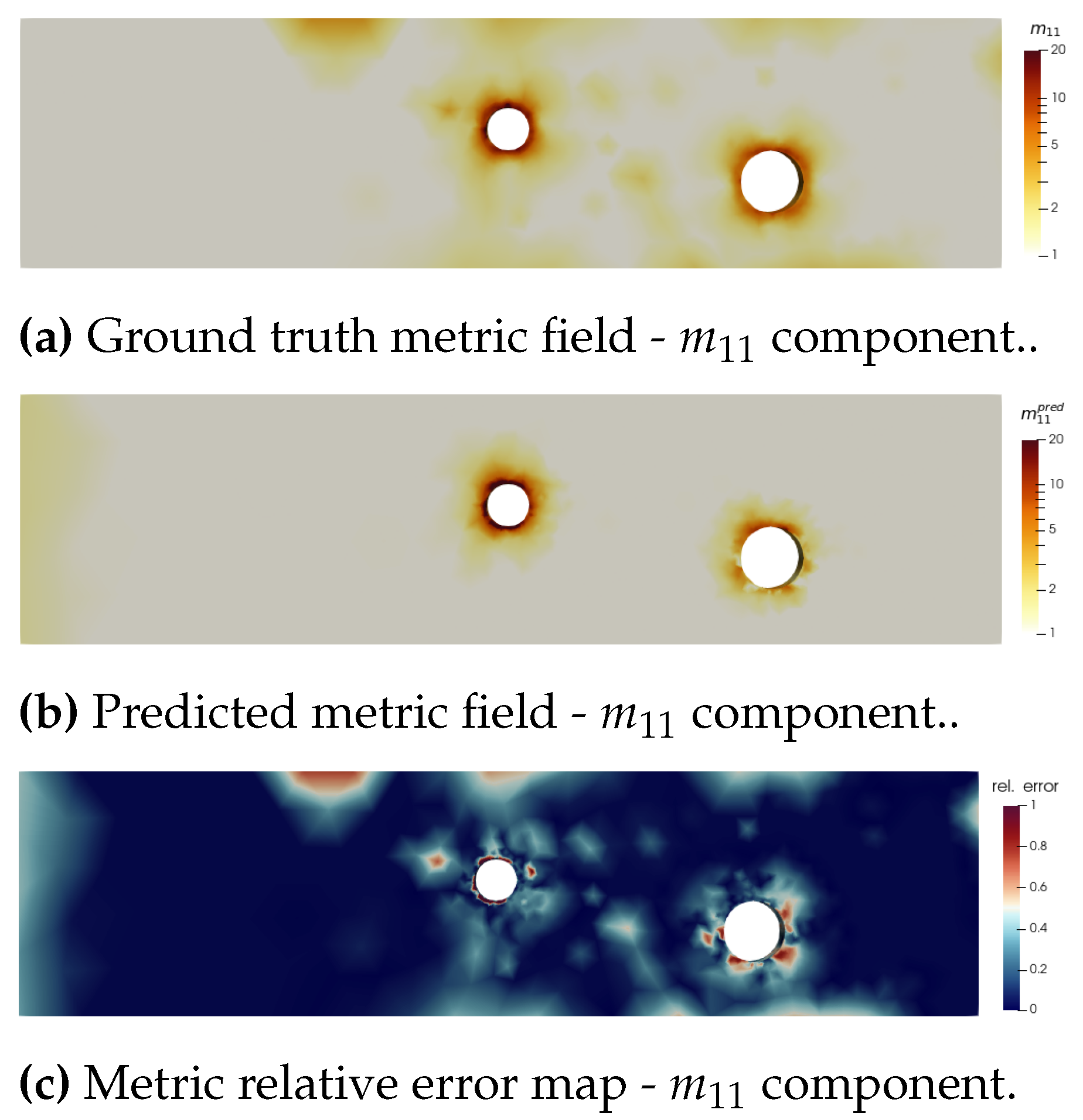
Figure 15. 3D mesh adaptation using Mmg for the ground truth metric field and the one predicted by Graphnet on simulation 106.

Figure 16. Quality of meshes predicted by Graphnet on simulations from the test set.

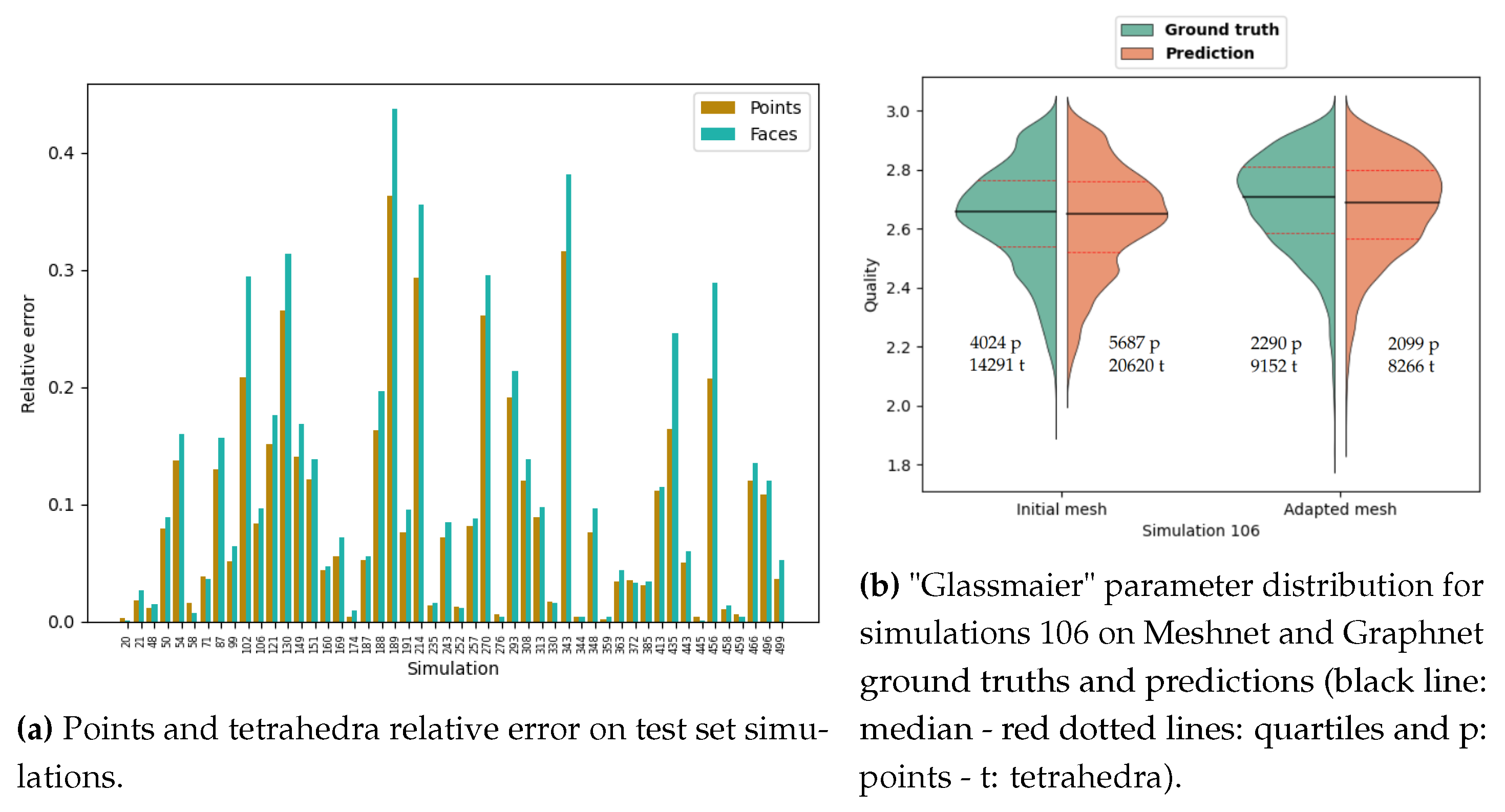
Figure 17. Generalisation of the Meshnet prediction for 3-hole geometry.

Figure 18. Generalisation of the Meshnet prediction for 3-hole geometry.

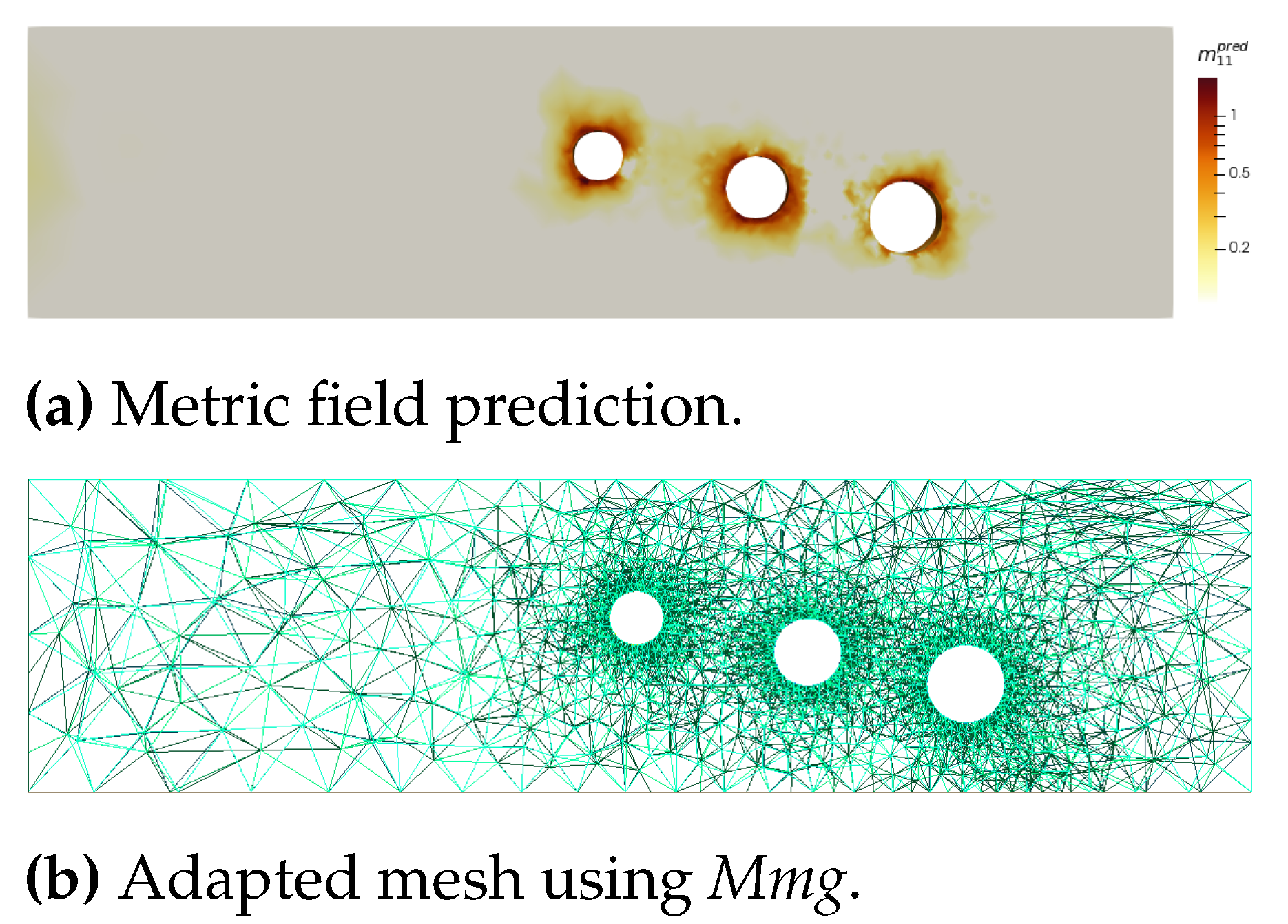
Figure 19. "Glassmaier" parameter distribution (black line: median - red dotted lines: quartiles) for Meshnet and Graphnet predictions.

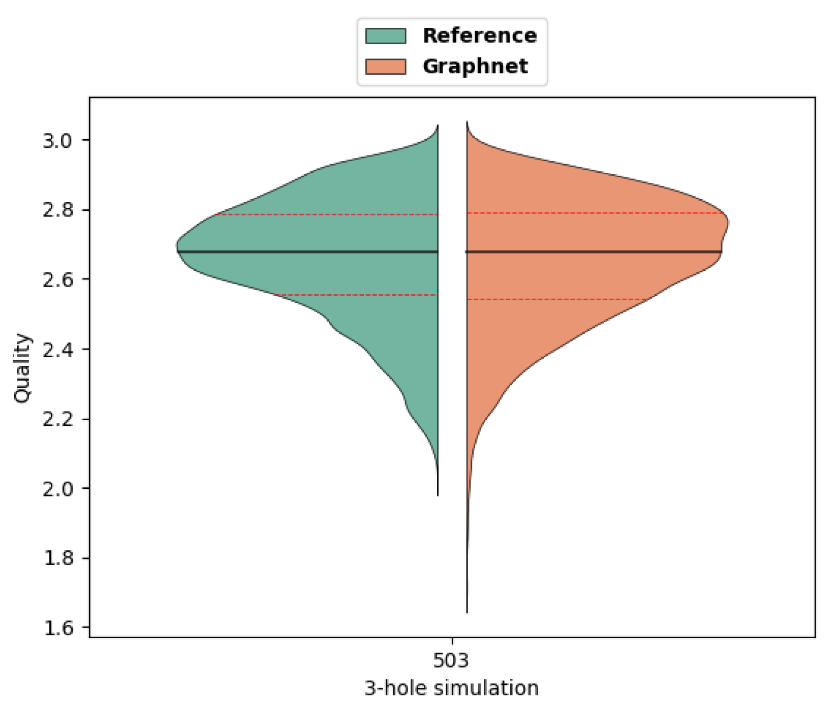
Figure 20. Generalisation of the Graphnet prediction for square geometry.

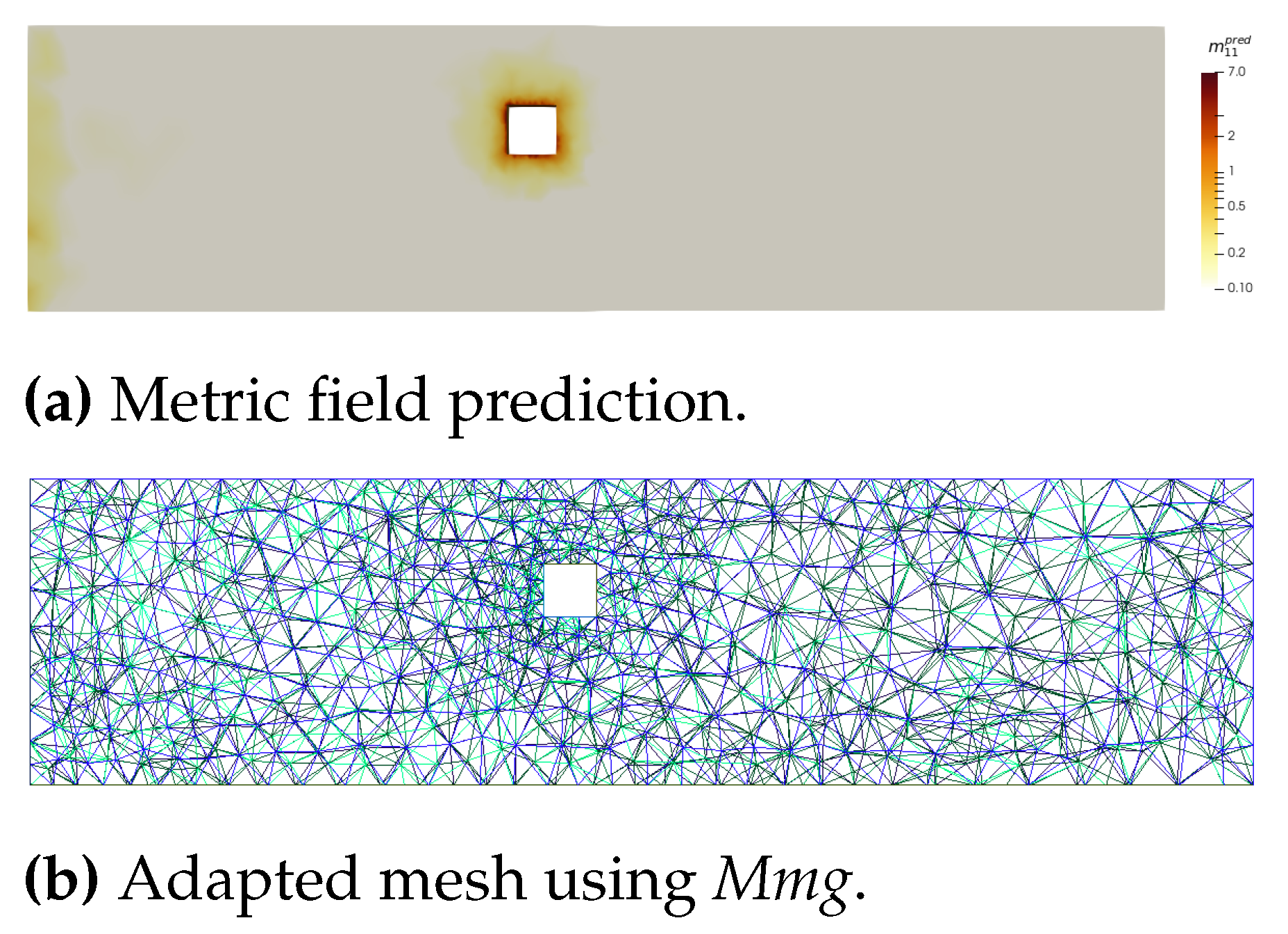
Figure 21. "Glassmaier" parameter distribution (black line: median - red dotted lines: quartiles) for Meshnet and Graphnet predictions.

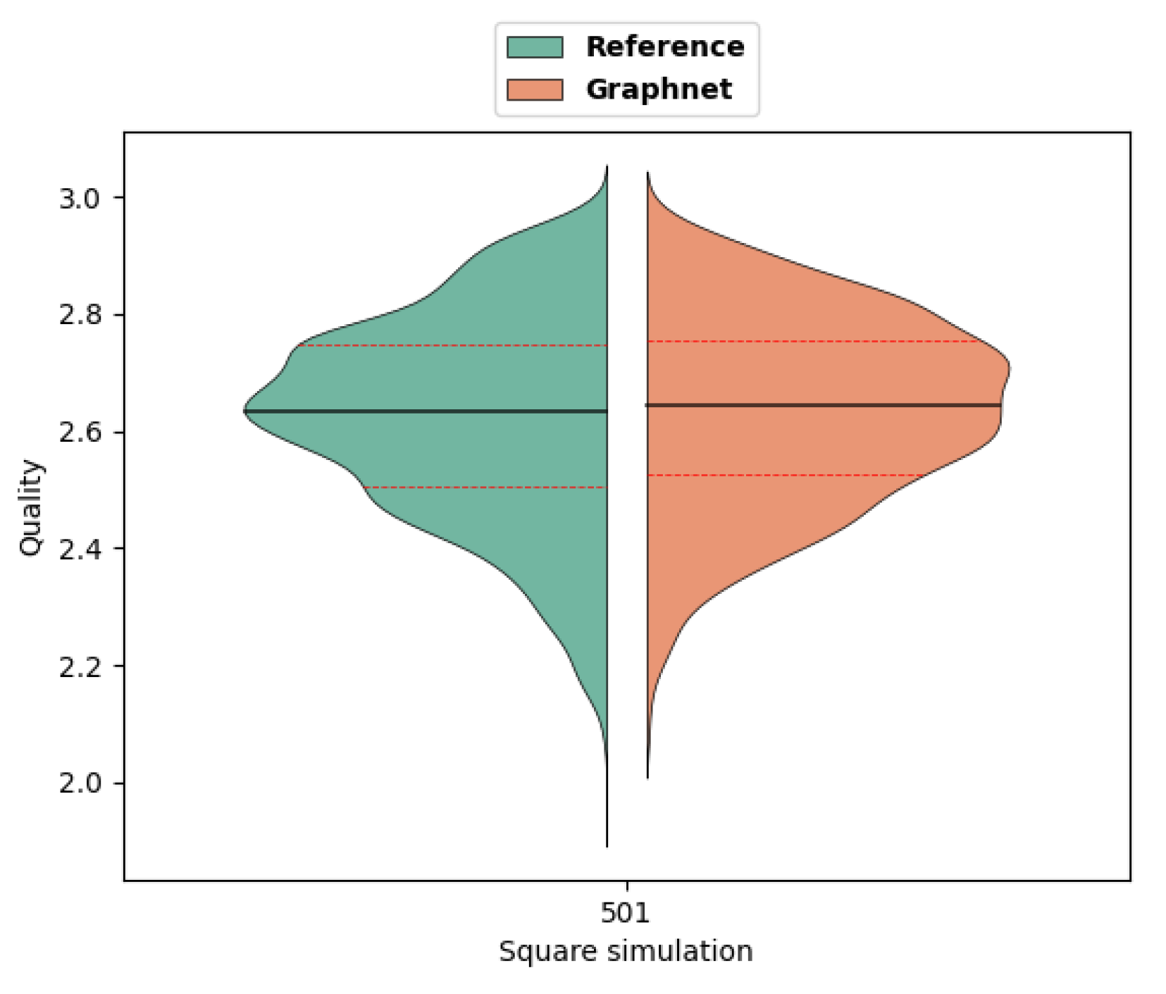
Figure 22. Training loss for the six components of the metric tensor. Each component was learnt independently by one specific network.

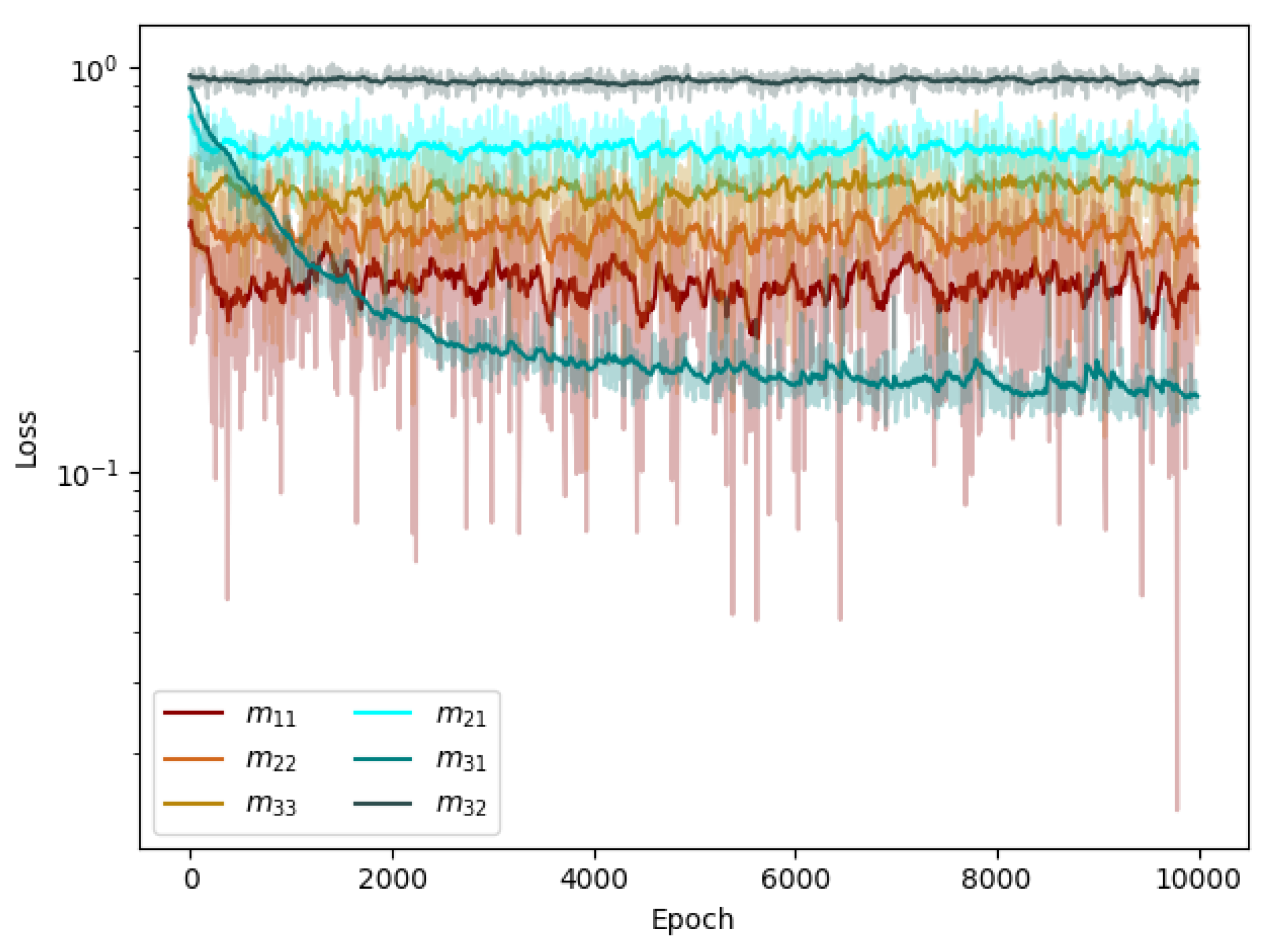
Figure 23. Graphnet prediction for 3-hole geometry.

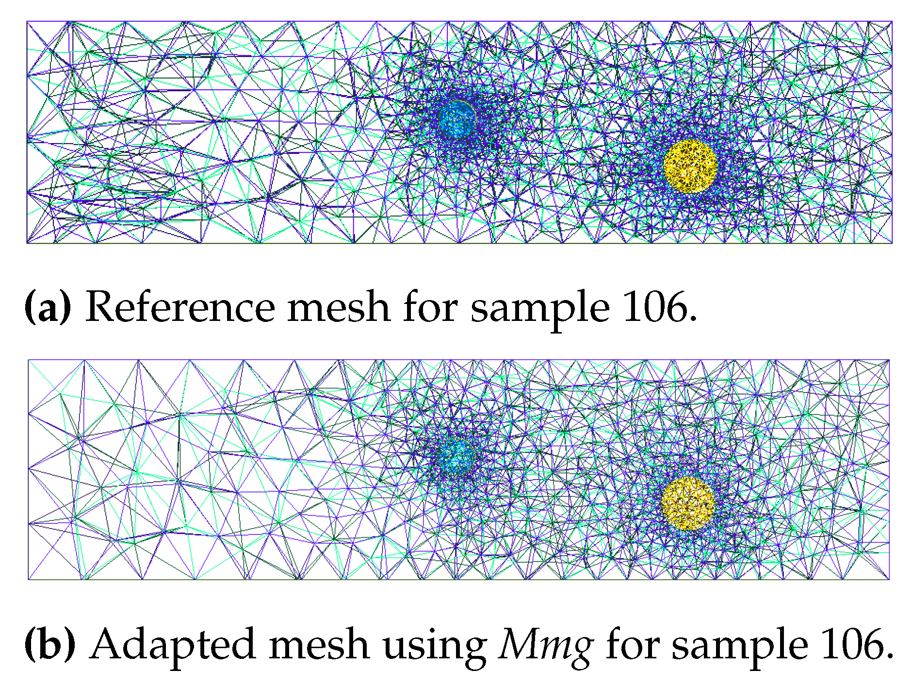
Figure 24. "Glassmaier" parameter distribution (black line: median - red dotted lines: quartiles) for Reference and Graphnet predictions.

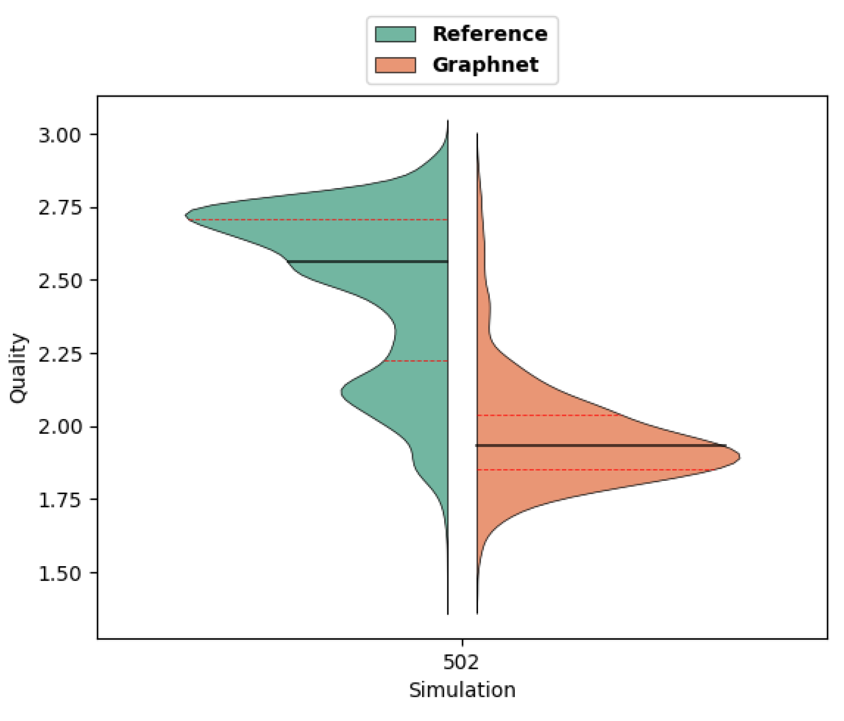
Table 1. Special values of the Glassmeier parameter.

$Q_{G}$	Meaning
$1.0$	The four points are colinear.
$2.0$	The four points all lie in a plane .
$3.0$	A regular tetrahedron is formed .

Table 2. Training duration for two different batch sizes.

Component	$m_{11}$	$m_{21}$	$m_{22}$	$m_{31}$	$m_{32}$	$m_{33}$
Duration (h)	$52.13$	$52.03$	$52.28$	$47.83$	$42.13$	$42.38$
Batch size	2	2	2	4	4	4

Table 3. CPU time comparison for computation and prediction of each phase.

Model	Meshnet	Graphnet
Computation	Engineer time	50.06s
Prediction	0.68s	0.79s
Speed-up	ND	63.4

Disclaimer/Publisher’s Note: The statements, opinions and data contained in all publications are solely those of the individual author(s) and contributor(s) and not of MDPI and/or the editor(s). MDPI and/or the editor(s) disclaim responsibility for any injury to people or property resulting from any ideas, methods, instructions or products referred to in the content.

© 2024 by the authors. Licensee MDPI, Basel, Switzerland. This article is an open access article distributed under the terms and conditions of the Creative Commons Attribution (CC BY) license (http://creativecommons.org/licenses/by/4.0/).

Copyright: This open access article is published under a Creative Commons CC BY 4.0 license, which permit the free download, distribution, and reuse, provided that the author and preprint are cited in any reuse.

MDPI Initiatives

Important Links

Choose an area of interest and we will send you notifications of new preprints at your preferred frequency.

Disclaimer

Graph Neural Networks for Mesh Generation and Adaptation in Structural and Fluid Mechanics

Abstract

1. Introduction

2. Materials and Methods

2.1. Problem Statement

2.1.1. Stokes Problem

2.1.2. Linear Elasticity Problem

2.2. Dataset

2.3. Mesh Parameters

2.4. Mesh-Based Simulations

2.5. Graph Representation

2.6. Model

2.6.1. Encoder

2.6.2. Processor

2.6.3. Decoder

2.6.4. Local and Global Features

2.7. Loss Function and Optimiser

3. Results

3.1. Meshnet

3.1.1. Fine Tuning Input Data for Message-Passing GNN

3.1.2. Evaluating Meshes Similarity and Quality

3.2. Graphnet

3.2.1. Direct Predictions: Velocity and Anisotropic Metric Fields

3.2.2. Mesh Adaptation

3.3. Adaptnet

4. Discussion

4.1. Meshnet Generalisation

4.2. Graphnet Generalisation

4.3. Linear Elasticity Problem

5. Conclusions

Author Contributions

Funding

Data Availability Statement

Acknowledgments

Conflicts of Interest

Abbreviations

Appendix A.

Appendix A.1. Linear elasticity problem

Appendix A.2. Model

References

MDPI Initiatives

Important Links

Subscribe