Submitted:
21 August 2024
Posted:
22 August 2024
You are already at the latest version
Abstract
Billions of euros are invested every year by professional football clubs for the recruitment of players. This article presents the latest advances in the statistical modelling of the factors that market actors take into consideration to determine the transfer prices of professional football players. It extends to a global scale the econometric approach previously developed by the authors to evaluate the transfer prices of players under contract with clubs from the five major European leagues. The statistical technique used to build the model is multiple linear regression (MLR), with fees paid by clubs as an independent variable. The sample comprises over 8000 transactions of players transferred for money from clubs worldwide during the period stretching from July 2014 to March 2024. This paper shows that a statistical model can explain almost 85% of the differences in the transfer fees paid for players. Despite the specific cases and other possible distortions mentioned in the discussion, the use of a statistical model to determine player transfer prices seems highly relevant.
Keywords:
football
; soccer
; transfer value
; transfer fees
; econometric model
; world
1. Introduction
This article presents the latest advances in the statistical modelling of the factors that market actors take into consideration to determine the transfer prices of professional football players. It extends to a global scale the econometric approach previously developed by the authors to evaluate the transfer prices of players under contract with clubs from the five major European leagues (Poli et al. 2022).
The new linear regression model implemented to account for the transfer values of professional football players is now based on 8,389 transactions, compared with 2,045 in the aforementioned article. The modification of certain variables and the inclusion of additional ones have enabled us to maintain an explanatory power equivalent to that previously achieved for far fewer observations, with a coefficient of determination of almost 85%.
This result confirms that price formation on the transfer market is more rational and statistically modellable than it is often thought by public opinion. Beyond the rumours spread by the media (Fürész and Rappai 2020; Herrero-Gutiérrez and Urchaga-Litago 2021; Runsewe et al. 2024) and players’ agents (Kelly and Chatziefstathiou 2017), our analysis confirms that it is possible to objectively identify the main factors involved in the transfer fee determination process.
While the weight of the various price determinants may vary from transaction to transaction, and non-modellable or quantifiable criteria may also play a role (Poli et al. 2022), as it will be further developed in the discussion, the rationales followed by transfer market actors are largely translatable into a statistical approach.
The pioneering publications on football players’ transfer values date back to the 1990s (Carmichael and Thomas 1993; Carmichael et al. 1999; Dobson and Gerrard 1999; Dobson et al. 2000). Many authors have then consolidated the existing literature, both before (notably Coates and Parshakov 2021; Garcia del Barrio and Pujol 2021; Majewski 2016; Müller et al. 2017; Ruijg and van Ophem 2015; Serna Rodríguez et al. 2018) and after (notably Campa 2022; Mc Hale and Holmes 2022; Franceschi et al. 2023a; Franceschi et al. 2023b) our own previous publication (Poli et al. 2022).
Academic interest in the statistical analysis of the determinants of professional football players’ transfer prices has grown in parallel with the increase in the sums involved. According to the official data published by FIFA TMS (2024) and those collected by the CIES Football Observatory research group, of which the authors are the founders, using the methodology presented in the aforementioned article (Poli et al. 2022), a new spending record was set in 2023.
2. Methodology
2.1. Sample
The sample from which the statistical model presented in this paper was built consists of 8,389 transfers having taken place between July 2014 and March 2024, involving 6,347 players. The number of transfers is greater than that of the footballers concerned as in 1,626 cases the latter experienced several fee-paying transfers included in the model, up to a maximum of seven for the Franco-Algerian striker Andy Delort.
The model’s dependent variable is the indemnity (fee) negotiated by the clubs at the time of the transfer, whether fixed or conditional (add-ons). Only transfers involving at least three quarters of the players’ economic rights were included, projected at 100% of the value. If transfers concerned less than three quarters of the economic rights, we considered that the price agreed was not necessarily thought of by market actors as a value proportional to the total value of the player at the time of the transfer, which justifies their exclusion from the sample.
Only permanent transfers have been taken into consideration. Transfers concluded after a loan period to the club with which the player was on loan were systematically excluded insofar as the amount of the compensation is in this case usually negotiated in advance by means of a clause. Similarly, paid transfers without a prior loan period concluded thanks to the retrieving of a buy-out clause in the player’s contract were not included in the sample.
By season, the number of transfers in the sample ranges from 539 in 2014/15 to 1,124 in 2023/24. The increase observed over the years, with the exception of the two seasons affected by the global health crisis (Poli et al. 2020), reflects both an increase in paying transactions, as illustrated in Figure 1, and an improvement in our own ability to collect the data needed to include transfers in the sample.
Figure 1.
Global transfer fee spending, € billion (2014-2023).
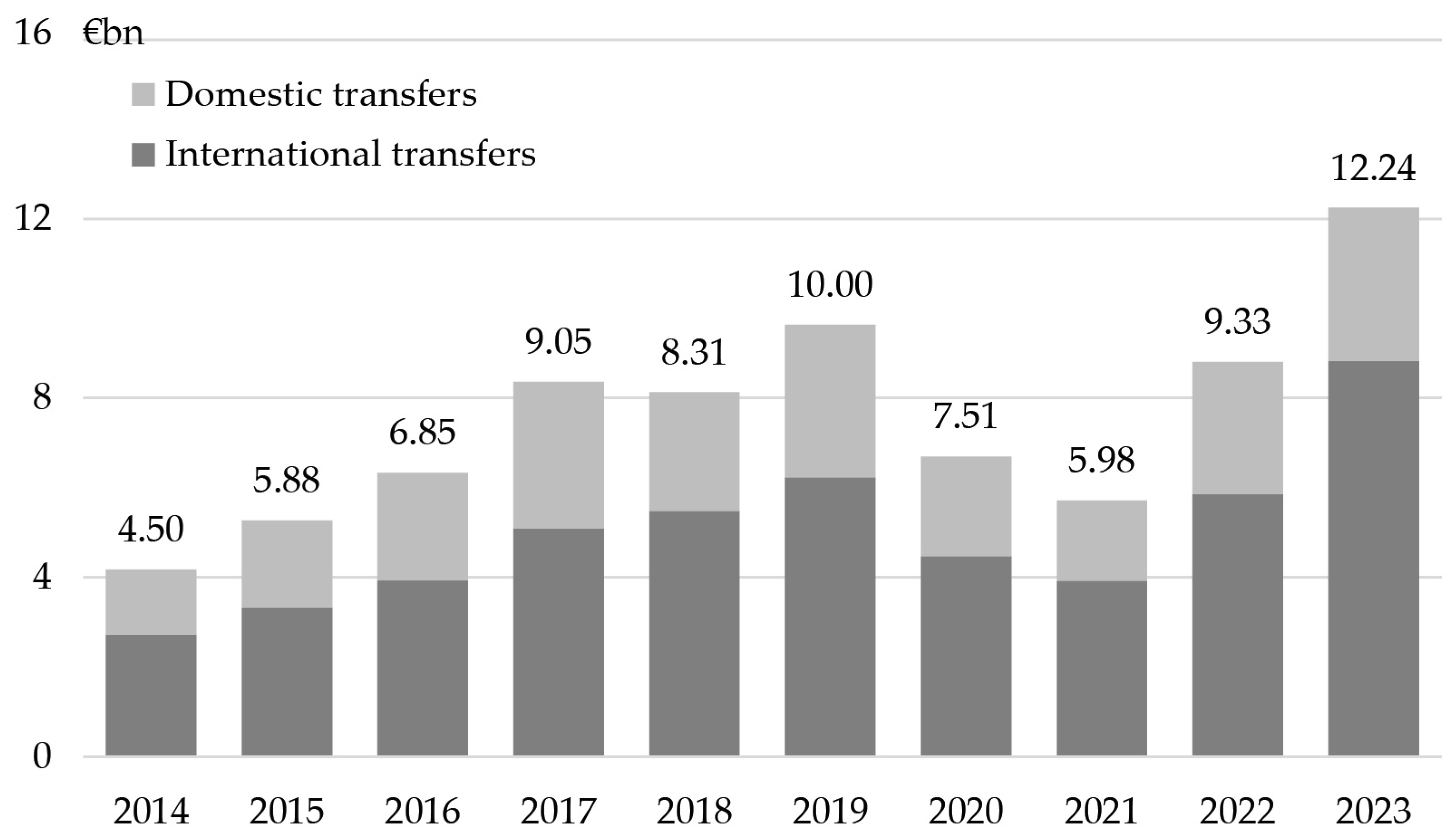

Table 1.
Sample per season of transfer.
| Year | Number |
|---|---|
| 2014 | 424 |
| 2015 | 622 |
| 2016 | 827 |
| 2017 | 897 |
| 2018 | 877 |
| 2019 | 904 |
| 2020 | 687 |
| 2021 | 662 |
| 2022 | 1019 |
| 2023 | 1168 |
| 2024 | 302 |
| 2014 | 424 |
| 2015 | 622 |
| 2016 | 827 |
| 2017 | 897 |
In terms of the number of transfers per association to which the releasing clubs belong, the countries with the richest leagues in the world (Frick et al. 2021) are in first place, namely England, France, Italy, Germany and Spain. National or international transfers from these associations account for 43% of the paid transactions in the sample, which reflects the centrality of these nations in the global football market. However, the sample includes transfers from no fewer than 54 national associations.
Table 2.
Sample per releasing association.
| Country | Number | Percentage |
|---|---|---|
| England | 895 | 10.7% |
| France | 750 | 8.9% |
| Italy | 732 | 8.7% |
| Germany | 718 | 8.6% |
| Spain | 509 | 6.1% |
| The Netherlands | 413 | 4.9% |
| Belgium | 357 | 4.3% |
| Argentina | 279 | 3.3% |
| Brazil | 278 | 3.3% |
| Portugal | 278 | 3.3% |
| 44 others | 3180 | 37.9% |
| Total | 8389 | 100.0% |
From the perspective of recruitment associations, the same countries mentioned above stand out. In this case, the over-representation of England is even more marked (16.7% of total incoming transfers compared to 10.7% of outcoming ones), reflecting the hold of English clubs over the global football players’ transfer market (FIFA TMS 2024). However, here too, the sample is fairly diversified, as it includes transactions to 61 different national associations.
Table 3.
Sample per recruiting association.
| Country | Number | Percentage |
|---|---|---|
| England | 1398 | 16.7% |
| Italy | 932 | 11.1% |
| Germany | 821 | 9.8% |
| France | 681 | 8.1% |
| Spain | 512 | 6.1% |
| Turkey | 362 | 4.3% |
| Belgium | 346 | 4.1% |
| The Netherlands | 242 | 2.9% |
| Russia | 241 | 2.9% |
| USA | 232 | 2.8% |
| 51 others | 2622 | 31.3% |
| Total | 8389 | 100.0% |
Almost half of the players whose transfers are included in the sample from which the multiple linear regression was developed are centre forwards (22.5%) or defensive/central midfielders (20.5%). In contrast, the proportion of goalkeepers is only 4.2%, reflecting the smaller number of players in this position in club squads. However, there are still enough goalkeepers (350) for the statistical model to take them into account.
Table 4.
Sample per player position.
| Country | Number | Percentage |
|---|---|---|
| Goalkeepers | 350 | 4.2% |
| Centre backs | 1449 | 17.3% |
| Full backs | 1014 | 12.1% |
| Defensive midfielders | 1719 | 20.5% |
| Attacking midfielders | 589 | 7.0% |
| Wingers | 1377 | 16.4% |
| Centre forwards | 1891 | 22.5% |
| Goalkeepers | 350 | 4.2% |
| Centre backs | 1449 | 17.3% |
| Total | 8389 | 100.0% |
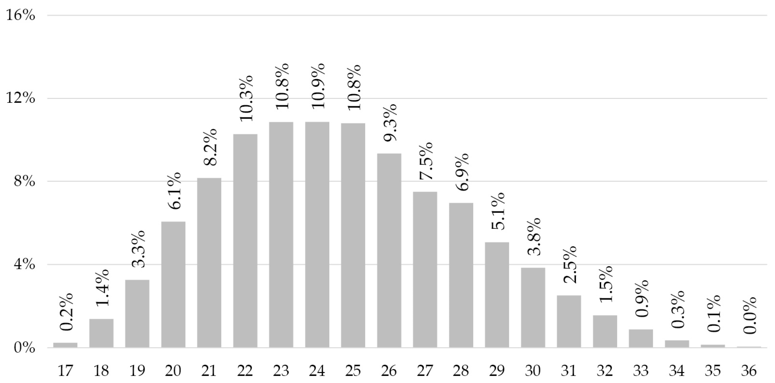
While the average age of players in the squads of professional football clubs worldwide is around 26.4 years (Poli et al. 2023b), the average for the footballers in the sample is 25.1 years. This discrepancy reflects the fact that younger players are more sought-after on the transfer market, and even more so when the transactions involve a financial compensation. Around 42% of the players in the sample were aged between 22 and 25 at the time of the transfer.
Figure 2.
Sample per age.
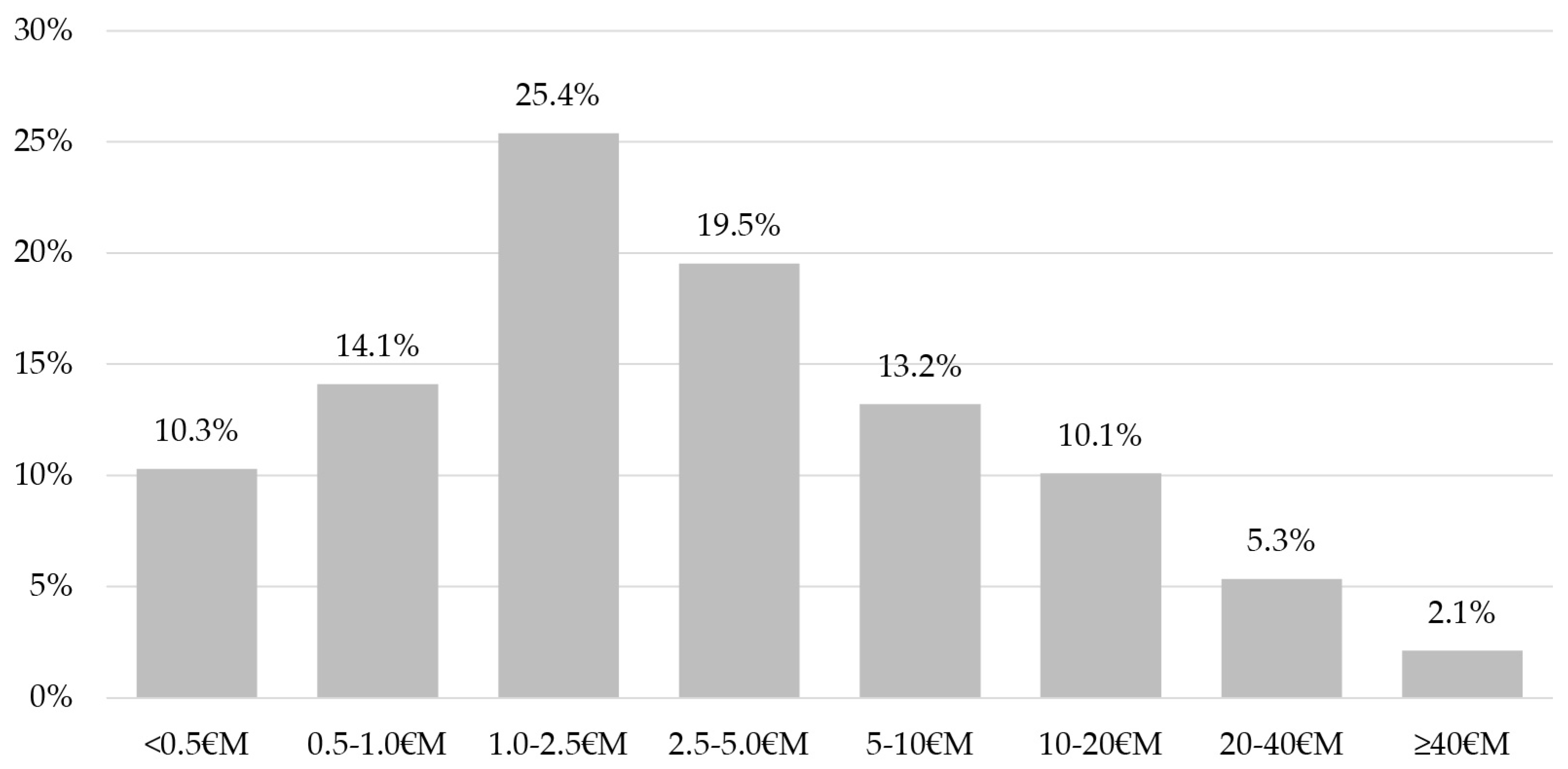
The vast majority of transfers on which the statistical model was built were concluded for a price of less than €20 million. Just over a quarter were negotiated for fees between €1 and €2.5 million (25.4%). Transactions for more than €20 million, on the other hand, are relatively infrequent, with a total of 626 observations, including only 178 for transfers in excess of €40 million. The asymmetry in the distribution of transfer indemnities implies their normalisation by a logarithmic transformation in order to explain them using a multiple linear regression.
Figure 3.
Sample per transfer fee category.
2.2. Variables
All the variables included in the model have a probability of error inferior to 5%. Numerous other variables were tested and ultimately not retained because they were either not significant (e.g. numerous technical gestures such as saves for goalkeepers, tackles, assists, etc.) or had too high a degree of collinearity with other variables.
Below, we introduce all the variables included in the multiple linear regression, explaining how they were calculated and the various issues that governed the choices made. Their relative weight in the formation of players’ prices is detailed in the following chapter.
Contract
Residual contract duration at the time of transfer, in days, maximum 1,825 days (i.e. 5 years). The value is transformed into a logarithm, which means that its impact on the transfer value increases as the end of the contract approaches (variable indicated by [contract] in the presentation of the statistical model in Table 5).
Age
Age of the player at the time of the transfer, without transformation, which implies that its impact on the transfer value is linear ([age] in Table 5).
Sporting level
Average sporting level of matches played by the footballer over the 365 days preceding the transfer ([level_s12] in Table 5) or between the 365th and 730th days preceding the transfer ([level_s34]). In order to calculate the sporting level of a match, for all players fielded, we compute all the games played in domestic leagues over the previous 365 days. Each minute played during this period is weighted by the sporting level of the corresponding league. The sporting level of a league is calculated on the basis of the sporting level of the corresponding national association, with a weighting according to the level of competition at domestic level (100% for the top division, 50% for the second, 25% for the third, etc.). Within a confederation, the sporting level of an association is calculated according to the results obtained by its representatives in international club competitions (Champions League, Copa Libertadores, etc.) over the last five years. In order to establish a single ranking worldwide, the highest-ranked association in each confederation is assigned the average sporting level of the best UEFA clubs to which players from the corresponding confederation were transferred in the last five years. The remaining associations are ranked according to the intra-confederation hierarchy.
Domestic minutes
Number of minutes played by the footballer in official national competition games (championships and cups) during the 365 days preceding the transfer ([mdom_s12] in Table 5) or between the 365th and 730th days preceding the transfer ([mdom_s34]).
International minutes
Number of minutes played by the footballer in official international competition games (clubs and A- or U21 national teams) in the 365 days preceding the transfer ([mint_s12] in Table 5) or between the 365th and 730th days preceding the transfer ([mint_s34]).
Goals
Number of goals scored by the footballer per 90 minutes played in club or national A- or U21 teams in the 365 days preceding the transfer ([goal_s12] in Table 5) or between the 365th and 730th days preceding the transfer ([goal_s34]).
Results
Average number of points obtained by the player’s teams (two points for a win, one for a draw and zero for a loss) in all official matches played by the footballer during the 365 days preceding the transfer ([ppm_s12] in Table 5) or between the 365th and 730th days preceding the transfer ([ppm_s34]).
Starting 11
Percentage of minutes played by the footballer as a starter in official club or national team matches (A- or U21) in the 365 days preceding the transfer ([start_s12] in Table 5).
Position
Position most occupied by the player in the six months preceding the transfer; binary variables (goalkeeper, centre back, full or wing back, central or defensive midfielder, attacking midfielder and winger), with centre forward as the reference value ([pos_gk], [pos_cb], [pos_fb], [pos_dm], [pos_am] and [pos_wi] in Table 5).
International status
Footballer who has played at least one match in his career for a national A-team at the time of the transfer ([inter] in Table 5).
Releasing club selling potential
Maximum income earned by the selling club over the last ten transfer periods adjusted to a reference value to capture the level of inflation at the time of the record income. The reference value is calculated on the basis of the average fee between the 10th and 100th most expensive transfers over the four years prior to the transfer window of the record income ([sel_club] in Table 5).
Releasing league selling potential
Average of the maximum income earned by each of the clubs from the selling league over the last ten transfer periods, adjusted to the reference value as above ([sel_leag] dans Table 5).
Destination club buying potential
Maximum expenditure of the buyer club over the last ten transfer periods, adjusted to the reference value as above ([buy_club] in Table 5).
Destination league buying potential
Average of the maximum expenditure of each of the clubs in the buying league over the last ten transfer periods, adjusted to the reference value as above ([buy_leag] in Table 5).
3. Results
3.1. Regression model
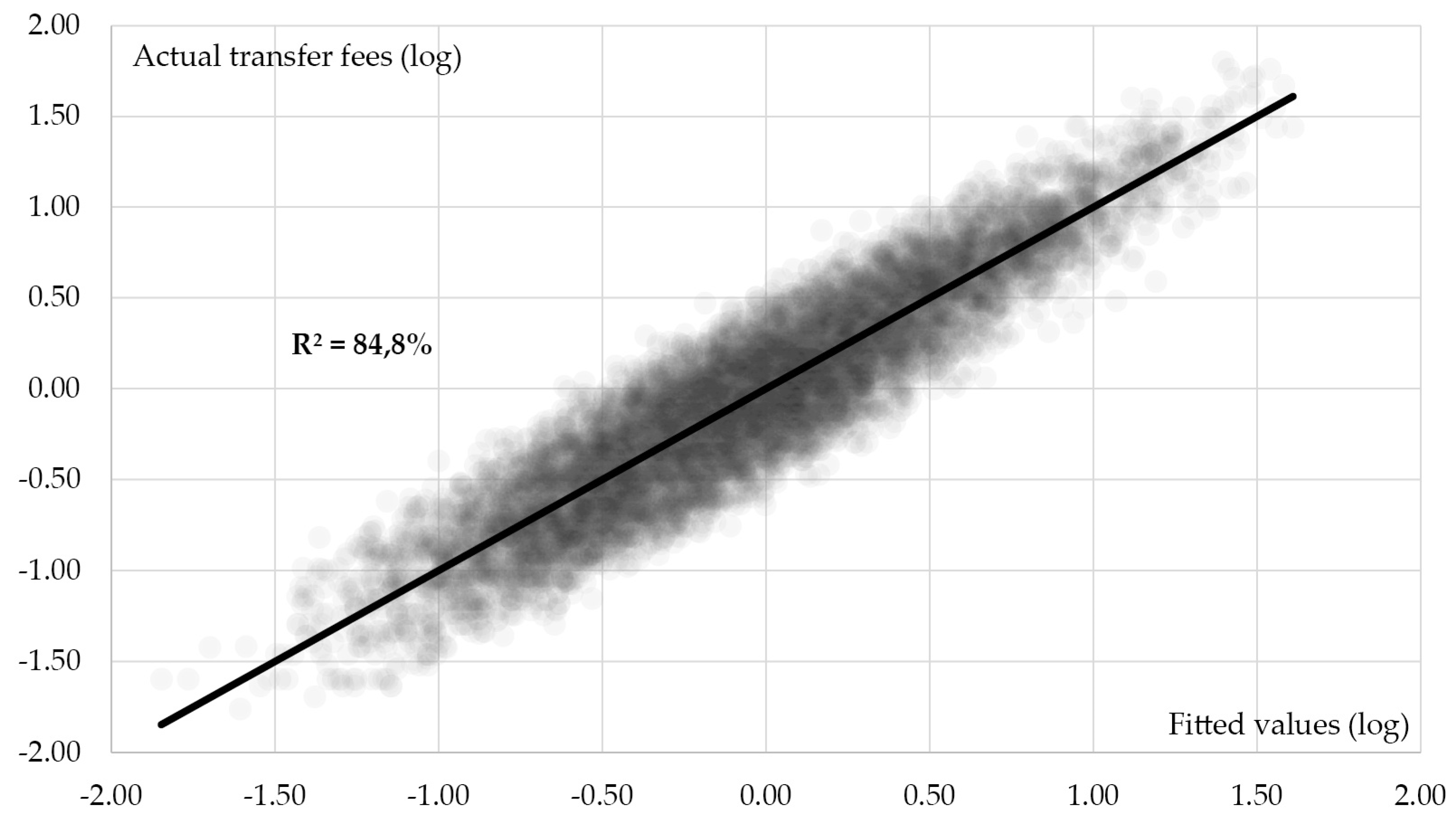
The regression model developed from the variables detailed above explains 84.8% of the differences in the fees paid for the 8,389 transfers included in the sample. As indicated, all the variables selected reach a level of significance greater than 95%. The t-value shows the relative weight of each variable in the determination of players’ prices.
With a t-value of 45.58, the remaining contract duration is an extremely important variable in the formation of players’ prices on the transfer market. It is transformed on a logarithmic scale, which implies that the shorter the remaining contract period, the greater its impact. As a matter of example, all other things being equal, when a player has four years remaining on his contract, one year less implies a 13% drop in his value, whereas the decrease is 29% if the footballer only had two years remaining on his contract.
The t-value is also very high for age, in this case with a negative sign (-51.09). Given their longer-term potential, younger players are comparatively better valued than older ones. The effect is linear, which means that a difference of five years will have the same impact (-44%) if we compare, for example, two players with identical profiles aged 18 and 23 years, or 28 and 33 years.
The variables that compare the position of players in relation to centre forwards all have negative coefficients, which indicates that centre forwards, all other things being equal, are the most valued. The most negative coefficient compared to centre forwards is recorded for full/wing backs, who have a value 16% lower than the reference category. On the other hand, the difference is very limited (not significant) for goalkeepers and attacking midfielders (on average around -3%).
Regarding all the variables referring to players’ performance, the most important is the sporting level of matches played, followed by the number of minutes played in the league, the number of goals scored and the tendency to be included in the starting 11s. In comparison, the results of matches played or the fact of playing international games, both for club or national teams, while also highly significant, are less important.
Whatever the variable, that referring to the most recent period (last 365 days) has systematically the highest t-value. This result indicates that the prices of players on the transfer market are formed essentially on the basis of their performances over the last year, with the previous year also playing a significant role, but to a much lesser extent. The tests carried out including previous years were all negative. International status, acquired once and for all, is another element that tends to increase the price paid for a footballer, by around a third, all other things being equal.
Finally, characteristics relating to the economic potential of both releasing and recruiting clubs form a last key group of factors. In this case, the variables referring to the destination club and league have a greater weight compared to those relating the club of departure. This finding reflects the overriding importance of the recruiters’ buying power in determining prices during negotiations.
Figure 4.
Fitted and actual transfer fees.
Correlation levels are also very high when observations are segmented according to different criteria. By period (Table 6), the coefficients of determination increase over time, suggesting a rationalisation of the market on the basis of the logics underlying the variables included in the statistical model. An improvement in the quality of the data gathered can also explain this development. The explanatory power of the model is relatively similar across all positions and age categories: between 83% and 87% (Table 7 and Table 8).
Table 6.
Coefficient of determination per period.
| Season | N | R2 |
|---|---|---|
| 2014/15-2015/16 | 1264 | 80.0% |
| 2016/17-2017/18 | 1741 | 83.7% |
| 2018/19-2019/20 | 1771 | 84.8% |
| 2020/21-2021/22 | 1418 | 84.5% |
| 2022/23-2023/24 | 2195 | 87.6% |
Table 7.
Coefficient of determination per player position.
| Country | N | R2 |
|---|---|---|
| Goalkeepers | 350 | 87.1% |
| Centre-backs | 1449 | 84.0% |
| Full-backs | 1014 | 85.2% |
| Defensive midfielders | 1719 | 85.2% |
| Attacking midfielders | 589 | 87.6% |
| Wingers | 1377 | 85.2% |
| Centre-forwards | 1891 | 83.1% |
Table 8.
Coefficient of determination per age category.
| Country | Number | Percentage |
|---|---|---|
| 21 years or less | 1599 | 83.4% |
| 22-25 years | 3587 | 85.6% |
| 26-29 years | 2419 | 84.2% |
| 30 years or more | 784 | 83.2% |
Cross-validation is another way of testing the quality and robustness of the model. To do this, the sample was randomly divided into five groups with the same number of individuals. Each time, a model was created with the transfers of four of these groups and the parameters were applied to predict the values of the fifth. The results obtained in terms of coefficients of determination are very stable (between 83% and 85%), both in terms of modelling and application.
Table 9.
5-fold cross-validation analysis for model to assess transfer fees.
| Training sample | Test sample | |||
|---|---|---|---|---|
| N | R2 adj | N | R2 adj | |
| Cross-validation 1 | 6712 | 84.70% | 1677 | 85.00% |
| Cross-validation 2 | 6711 | 84.81% | 1678 | 84.57% |
| Cross-validation 3 | 6711 | 84.71% | 1678 | 84.97% |
| Cross-validation 4 | 6711 | 85.05% | 1678 | 83.54% |
| Cross-validation 5 | 6711 | 84.59% | 1678 | 85.46% |
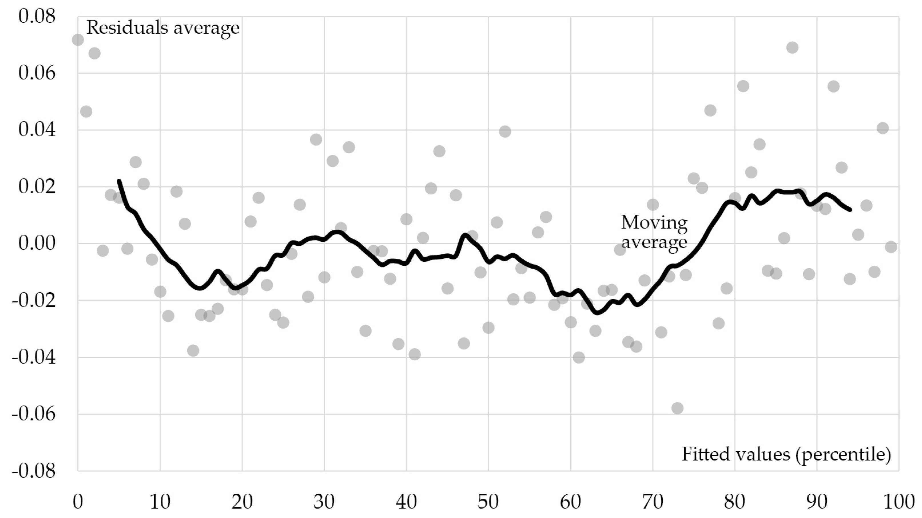
On a global scale, the scatter plot linking the model’s estimates and the residuals does not show any particular shape, which rules out any flagrant problem of heteroscedasticity. The application of statistical tests such as the White or Breusch-Pagan test does not validate the hypothesis of the homoscedasticity of the variance of the residuals. The model tends indeed to slightly underestimate the values in the most extreme spectra, while the values for certain intermediate segments are slightly overestimated.
Figure 5.
Estimates’ and residuals’ scatter plot.
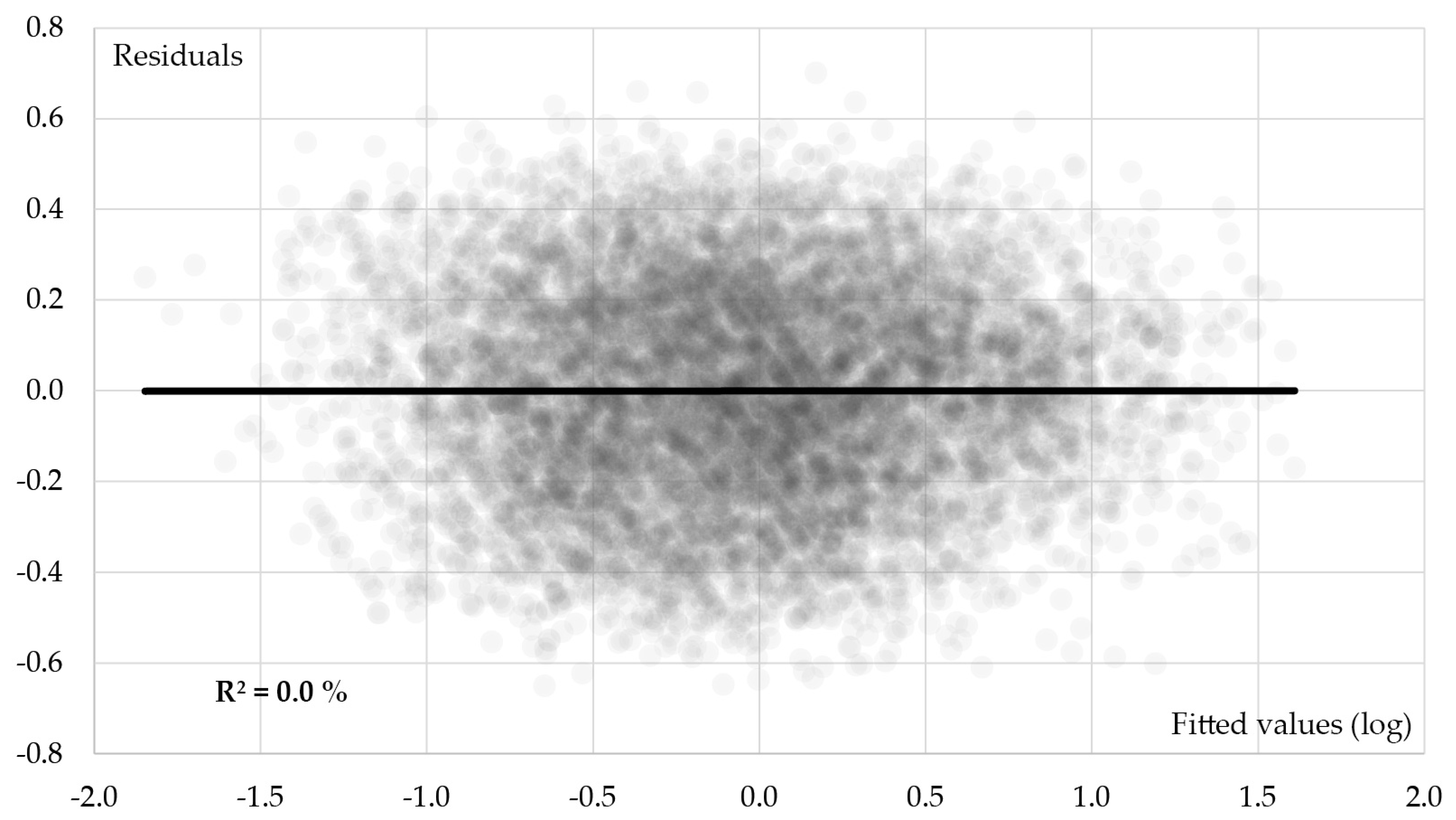
Figure 6.
Average residuals, as per estimate in percentile.
4. Discussion
Although our regression model for assessing the transfer price of professional football players is particularly robust and effective, some of the prices paid by clubs differ significantly from the estimated values. Below, we present some of the main discrepancies observed, which allows us to account for certain specific or statistically non-modellable criteria that may nevertheless have an impact on the price determination process.
The transfer of the Brazilian striker Hulk Givanildo from Zenit St. Petersburg to Shanghai Port in 2016 was negotiated at a price almost four times higher than that estimated by our statistical model. Part of the discrepancy can be explained by the fact that Chinese clubs had previously not been very active on the transfer market. Consequently, their economic potential as integrated into the model, calculated on the basis of past transactions, lagged behind.
In addition, as in the case of other countries or clubs stepping up their recruitment to acquire a more central role in the football economy, overpaying players and their former clubs is often an essential condition for transfers to go through. Finally, it cannot be ruled out that the very fact of paying large sums is valued by the emerging recruiting countries or clubs as a signal of their new status and ambition, which does not encourage them to negotiate prices downwards.
The transfer of Willem Geubbels from Olympique Lyonnais to Monaco in 2018 was also negotiated at a much higher price than estimated. Geubbels was a very young player who had already shone at youth level, so much so that he was considered to have similar potential to Kylian Mbappé, who is two and a half years older and was transferred by Monaco to PSG in the same transfer window for €180m including add-ons. However, Geubbels had played very little at professional level up to that point, which makes our model less suitable for evaluating him, insofar as the vast majority of the transactions on which he was built involved players with at least one-year experience at adult level.
An opposite case, where the value was overestimated, is for example that of the transfer of striker Mario Balotelli from Milan to Liverpool in 2014, negotiated at half the estimated value. The Italian’s disciplinary problems may explain this discrepancy, as they are for other players whose behaviour does not offer the best guarantees to recruiting clubs. This has a negative and non-modellable impact on the fees that clubs are willing to invest to sign them.
Other cases also involve aspects that are difficult to model. The financial difficulties of the clubs to which players belong can have a negative impact on transfer prices, as was notably the case in the summer of 2024 for Girondins de Bordeaux, a French club that went into administration. In such cases, deals can be heavily cut to generate money in the short term.
Financial accounting needs may also explain some of the discrepancies observed in certain transactions, in particular those carried out in a hurry before the annual accounts are closed. This can result either in transfers on the cheap (for example, Mohammed Salah’s transfer from Rome to Liverpool in June 2017) or, on the contrary, overpaid transfers and swap deals raising suspicions of accounting manipulation and collusion between clubs (in summer 2024, among other cases, Nottingham Forest and Olympique Lyonnais, Everton and Newcastle United, Aston Villa and Chelsea, etc.).
Other cases involve teams that have been relegated or have speculated on promotion but have failed to achieve it, and are therefore forced to drastically reduce their wage bill, sometimes at the cost of having to sell off players in order to balance their books and avoid spiralling into debt. From this point of view, if it was available on a large scale, the variable of the player’s salary would certainly provide an addition to the statistical model developed.
Despite these specific cases and other possible distortions, our approach shows that it is possible to use a statistical model to account for the way in which market actors determine player transfer prices. The various tests carried out by segmenting the sample by period show that these criteria are relatively stable over time, albeit with some changes.
Since the health crisis, for example, the age factor has become even more discretising, with an increasing number of clubs targeting their recruitment on young talent in order to make capital gains through their subsequent transfer, which has led to higher inflation for players under 23 than for older footballers (Poli et al. 2023a).
The approach presented is particularly effective for assessing the fair price of players after their transfer. From a predictive perspective, when the acquiring club is not known, in order to determine an expected amount, it is however necessary to develop another statistical model with the financial strength of the likely acquirer as the dependent variable. Various tests were also carried out for this purpose, which enabled us to achieve a coefficient of determination of around 65%, with certainly still room for improvement.
Author Contributions
Conceptualization, R.P.; Data curation, R.B. and L.R.; Formal analysis, R.B.; Investigation, R.P. and R.B.; Methodology, R.B.; Project administration, R.P.; Resources, L.R.; Supervision, L.R.; Validation, L.R.; Writing—original draft, R.P.; Writing—review & editing, R.P. and R.B. All authors have read and agreed to the published version of the manuscript.
Funding
This research received no external funding
Acknowledgments
The authors warmly thank the CIES direction and colleagues for their continuous support over the years.
Conflicts of Interest
The authors declare no conflict of interest.
References
- (Campa and Domenico 2022) Camp and Domenico 2022. Exploring the Market of Soccer Player Registrations: An Empirical Analysis of the Difference Between Transfer Fees and Estimated Players’ Inherent Value. Journal of Sports Economics. 23 (4): 1–28. [CrossRef]
- (Carmichael and Thomas 1993) Carmichael, Fiona, and Dennis Thomas. 1993. Bargaining in the Transfer Market: Theory and Evidence. Applied Economics 25: 1467–76. [CrossRef]
- (Carmichael et al. 1999) Carmichael, Fiona, David Forrest, and Robert Simmons. 1999. The Labour Market in Association Foot-ball: Who Gets Transferred and For How Much? Bulletin of Economic Research 51: 125–50. [CrossRef]
- (Coates and Parshakov 2021) Coates, Dennis, and Petr Parshakov. 2021. The wisdom of crowds and transfer market values. European Journal of Operational Research. 301 (2): 523–34. [CrossRef]
- (Dobson and Gerrard 1999) Dobson, Stephen, and Bill Gerrard. 1999. The determination of player transfer fees in English professional soccer. Journal of Sport Management 13: 259–79. [CrossRef]
- (Dobson et al. 2000) Dobson, Stephen, Bill Gerrard, and Simon Howe. 2000. The determination of transfer fees in English non-league football. Applied Economics 32: 1145–52. [CrossRef]
- (FIFA TMS 2024) FIFA TMS. 2024. Global Transfer Report 2023. Zurich: FIFA. Available online: https://digitalhub.fifa.com/m/114622e4e17cf6a8/original/FIFA-Global-Transfer-Report-2023.pdf (fifa.com) (accessed on 25.17.2024).
- (Franceschi et al. 2023) Franceschi, Maxence, Jean-François Brocard, Florian Follert, and Jean-Jacques Gouguet. 2023. Determinants of football players’ valuation. A systematic review. Journal of Economic Surveys 38 (3): 577–600. [CrossRef]
- (Franceschi et al. 2023b) Franceschi, Maxence, Jean-François Brocard, Florian Follert, and Jean-Jacques Gouguet. 2023. Football players in light of economic value theory: Critical review and conceptualisation. Managerial and Decision Economics 2: 896–920. [CrossRef]
- (Frick et al. 2021) Frick, Bernd, Tommy Kweku Quansah, and Markus Lang. 2023. Talent concentration and competitive imbalance in European soccer. Frontiers in Sports and Active Living 5: 1148122. [CrossRef]
- (Fürész and Rappai 2020) Fürész, Diána I., and Gábor Rappai. 2020. Information leakage in the football transfer market. European Sport Management Quarterly, 1–21. [CrossRef]
- (Garcia del Barrio and Pujol 2021) Garcia del Barrio, Pedro, and Francesc Pujol. 2021. Recruiting talent in a global sports market: Appraisals of soccer players’ transfer fees. Managerial Finance 47: 789–811. [CrossRef]
- (Herrero and Urchaga-Litago 2021) Herrero-Gutiérrez, Francisco-Javier, and José David Urchaga-Litago. 2021. The importance of rumours in the Spanish Sports Press: An Analysis of news about signings appearing in the newspapers Marca, As, Mundo Deportivo and Sport. Publications, 9 (1), 9. [CrossRef]
- (Kelly and Chatziefstathiou 2017) Kelly, Seamus, and Dikaia Chatziefstathiou. 2017. ‘Trust me I am a football agent’. the discursive practices of the players’ agents in (un)professional football. Sport in Society, 21(5): 800–814. [CrossRef]
- (Majewski 2016) Majewski, Sebastian. 2016. Identification of Factors Determining Market Value of the Most Valuable Football Players. Journal of Management and Business Administration 24: 91–104. [CrossRef]
- (McHale and Holmes 2022) McHale, Ian, and Benjamin Holmes. 2022. Estimating transfer fees of professional footballers using advanced performance metrics and machine learning. European Journal of Operational Research 306: 389–399. [CrossRef]
- (Müller et al. 2017) Müller, Oliver, Alexander Simons, and Alexander Weinmann. 2017. Beyond Crowd Judgments: Data-Driven Estimation of Market Value in Association Football European. European Journal of Operational Research 263: 611–24. [CrossRef]
- (Poli et al. 2020) Poli, Raffaele, Roger Besson, and Loïc Ravenel. 2020. The Real Impact of COVID on the Football Players’ Transfer market. Neuchâtel: CIES. Available online: https://football-observatory.com/IMG/sites/mr/mr58/en (accessed on 15.07.2024).
- (Poli et al. 2022) Poli, Raffaele, Roger Besson, and Loïc Ravenel. 2022. Econometric Approach to Assessing the Transfer Fees and Values of Professional Football Players. Economies 10, 4. [CrossRef]
- (Poli et al. 2023a) Poli, Raffaele, Roger Besson, and Loïc Ravenel. 2023. Inflation in the football players’ transfer market (2013/14-2022/23). Neuchâtel: CIES. Available online: https://football-observatory.com/IMG/sites/mr/mr82/en (accessed on 26.07.2024).
- (Poli et al. 2023b) Poli, Raffaele, Roger Besson, and Loïc Ravenel. 2023. Team demographics in 48 leagues worldwide. Neuchâtel: CIES. Available online: https://football-observatory.com/IMG/sites/mr/mr89/en (accessed on 26.07.2024).
- (Runsewe et al. 2024) Runsewe, Ife, Majid Latifi, Mominul Ahsan, and Julfikar Haider. 2024. Machine Learning for Predicting Key Factors to Identify Misinformation in Football Transfer News. Computers 13, 127. [CrossRef]
- (Ruijg and van Ophem 2015) Ruijg, Jeroen, and Hans van Ophem. 2015. Determinants of football transfers. Applied Economics Letter 22: 12–19. [CrossRef]
- (Serna Rodríguez et al. 2018) Serna Rodríguez, Maribel, Andrés Ramírez Hassan, and Alexander Coad. 2018. Uncovering Value Drivers of High Performance Soccer Players. Journal of Sports Economics 20: 1–31. [CrossRef]
Table 5.
Multiple linear regression to explain transfer fees.
| Country | b | t | prob | sign |
|---|---|---|---|---|
| [contrat] | 0.48 | 45.58 | 0.000 | *** |
| [age] | -0.05 | -51.09 | 0.000 | *** |
| [pos_gk] | -0.01 | -0.76 | 0.445 | ns |
| [pos_cb] | -0.03 | -2.28 | 0.023 | * |
| [pos_fb] | -0.08 | -5.89 | 0.000 | *** |
| [pos_dm] | -0.02 | -1.99 | 0.046 | * |
| [pos_am] | -0.01 | -1.08 | 0.281 | ns |
| [pos_wi] | -0.02 | -2.31 | 0.021 | * |
| [level_s12] | 1.51 | 33.53 | 0.000 | *** |
| [level_s34] | 0.41 | 12.44 | 0.000 | *** |
| [mindom_s12] | 0.01 | 22.93 | 0.000 | *** |
| [mindom_s34] | 0.00 | 5.18 | 0.000 | *** |
| [minint_s12] | 0.00 | 7.32 | 0.000 | *** |
| [minint_s34] | 0.00 | 5.27 | 0.000 | *** |
| [goal_s12] | 2.96 | 18.05 | 0.000 | *** |
| [goal_s34] | 0.82 | 5.37 | 0.000 | *** |
| [ppm_s12] | 0.21 | 8.90 | 0.000 | *** |
| [ppm_s34] | 0.05 | 2.55 | 0.011 | * |
| [start_s12] | 0.44 | 12.29 | 0.000 | *** |
| [inter] | 0.07 | 12.32 | 0.000 | *** |
| [selclub] | 0.13 | 10.18 | 0.000 | *** |
| [selleag] | 0.27 | 16.89 | 0.000 | *** |
| [buyclub] | 0.51 | 37.34 | 0.000 | *** |
| [buyleag] | 0.34 | 29.33 | 0.000 | *** |
| [cons] | -3.66 | -68.07 | 0.000 | *** |
Disclaimer/Publisher’s Note: The statements, opinions and data contained in all publications are solely those of the individual author(s) and contributor(s) and not of MDPI and/or the editor(s). MDPI and/or the editor(s) disclaim responsibility for any injury to people or property resulting from any ideas, methods, instructions or products referred to in the content. |
© 2024 by the authors. Licensee MDPI, Basel, Switzerland. This article is an open access article distributed under the terms and conditions of the Creative Commons Attribution (CC BY) license (http://creativecommons.org/licenses/by/4.0/).
Copyright: This open access article is published under a Creative Commons CC BY 4.0 license, which permit the free download, distribution, and reuse, provided that the author and preprint are cited in any reuse.


