
Submitted:
12 August 2024
Posted:
12 August 2024
You are already at the latest version
Abstract
Cascading landslides represent a dynamic and hazardous geological phenomenon, char-15 acterized by a sequential chain of slope failures triggered by various factors such as heavy rainfall, 16 seismic activity, or anthropogenic activities. These events can amplify the damage caused by the 17 initial trigger and propagate instability along a slope, often resulting in significant environmental 18 and societal impacts. The Morino-Rendinara cascading landslide, situated in the Ernici mountains 19 along the border of Abruzzo and Lazio region (Italy), serves as a notable example of the complexities 20 and devastating consequences associated with such events. In March 2021, a substantial debris flow 21 event in Morino obstructed the Liri River, marking the latest step in a series of landslide events 22 characterized by a complexity far beyond initial expectations. This study employs a multidiscipli-23 nary approach, combining conventional techniques and advanced technologies, to understand the 24 complexities of the Morino-Rendinara landslide. Field activities, UAV image acquisition, SAR inter-25 ferometry based on SENTINEL-1 images and pixel offset analysis based on high-resolution Google 26 Earth images, offer insights into the geological and hydrogeological setting of the unstable slope, 27 landslide geometry, mechanism and kinematics. To supplement the analysis a specific FEM slope 28 stability analyses is used to reconstruct the deep geometry of the system emphasizing the modula-29 tion action of groundwater flow to the slope stability
Keywords:
Cascading landslides
; Slope stability
; InSAR interferometry
; Pixel Offset
; Finite element 31 Analysis
; Numerical Modelling
1. Introduction
Cascading landslides can be described as series of landslides that occur sequentially in a chain reaction, typically initiated by a triggering event such as heavy rainfall, seismic activity, or anthropogenic activities such as excavation or blasting. This phenomenon starts when an initial landslide destabilizes the surrounding terrain, leading to sub-sequent landslides that may intensify the damage caused by the initial event or create a predisposed environment for subsequent slope failures [1]. These subsequent landslides can be triggered by slope overloading caused by debris generated by the initial event or changes in the terrain conditions resulting from an initial landslide [2]. As a result, cascading landslides can amplify the damage caused by the initial event and propagate the instability along a slope; common consequences of cascading landslides are landslide dams with consequent flooding [3]. Notable examples of this kind of process have been observed during the Nepal 2015 earthquake. On April 25th, 2015, in Lamjung (Nepal), a magnitude 7.8 earthquake triggered a series of landslides across large mountainous areas of the country, blocking rivers, causing floods, and resulting in considerable damage and human loss [4]. The scale and nature of the initial triggering event, as well as local geological conditions, the involved material and saturation condition, played a significant role in determining the velocity and impact of the cascading landslides. For example, heavy rainfall can saturate the soil, increasing its weight and reducing its stability, while seismic activity can lead to ground shaking, further destabilizing the slope. As predisposing factor wildfires can reduce the infiltration capacity of the slope and modify significant the trend and time of saturation capacity thus influencing the stability factor [5]. Mechanisms can include sliding, which occurs when a layer of soil moves along a sliding plane, often favoring clayey or highly saturated soils, and rolling, which involves the movement of larger debris, such as rocks or boulders, along the surface of the terrain. Bouncing is another mode that can occur, particularly with smaller or irregularly sized debris, where the de-bris bounces or hops along the surface of the terrain, propelled by the force of the flow [6]. During a cascading landslide, the debris and sediment generated by the initial landslide can be transported in different modes or flow regimes, depending on the characteristics of the terrain and the involved materials. Gravity-driven flow is a common mode of debris transport, where sediments move downslope under the influence of gravity. The velocity of the flow can vary, depending on factors such as the amount of water present in the de-bris and the slope of the terrain [7]. The transport of debris and sediment can significantly alter the shape and characteristics of the surrounding terrain. Debris accumulation can obstruct watercourses, roads, or inhabited areas, posing a threat to infrastructure and human populations. The movement of debris can also lead to erosion of the surrounding terrain, causing soil loss and changes in local topography. Additionally, cascading landslides can interact with existing infrastructure along their path, increasing the risk of damage and human loss. Buildings, bridges, roads, and other infrastructure can be impacted by subsequent landslides [8], resulting in structural damage or even destruction. Debris deposits can also block roads, railways, or watercourses, disrupting communication routes and hampering rescue and evacuation efforts [9]. The fast movement of debris and sediment poses a risk to human safety, as people along the path of cascading land-slides can be injured or killed [10]. The velocity of cascading landslides exhibits significant variability depending on the mechanisms involved in the slope failure process. Factors such as slope gradient, involved material (kind and volume), and triggering factor play crucial roles in determining the velocity of movement [11]. Landslides initiated by shallow translational sliding or surface erosion tend to move at slower velocities, typically ranging from centimeters to meters per year. In contrast, events triggered by rapid failure mechanisms such as rockfall, debris flow, or liquefaction can attain velocities exceeding 10 m/s. Moreover, the presence of water, either from precipitation or groundwater, can further in-fluence landslide velocity by increasing the weight of the sliding mass and reducing frictional resistance [8]. Notable examples highlight the destructive potential of cascading landslides are Kedarnath (Indian Himalayas); here in 2013, heavy rainfall caused a series of landslides and floods, destroying entire villages and thousands of deaths [12]. In 2017, Sierra Leone experienced a series of landslides triggered by heavy rainfall, causing a high number of casualties and widespread destruction of homes and infrastructure [13]. A further example is the Morino-Rendinara landslide [14]. This landslide develops along the Ernici mountains, near the border between Abruzzo and Lazio regions, in the Apennines Mountain range, typical environment where cascading landslides can be observed in Italy. The Morino-Rendinara cascading landslide (Figure 1) is one of the most significant examples of cascading landslide in terms of landslide mechanism differentiation, impact, and the involved surface. The study of the Morino-Rendinara landslide aims to comprehensively understand the kinematics of this cascading landslide, focusing on the mechanisms characterizing its components. The study of the Morino-Rendinara landslide aims to comprehensively understand the kinematics of this cascading landslide by focusing on the mechanisms characterizing its components. This is achieved through the integration of remote sensing techniques, the Finite Element Analysis (FEA) [15], and traditional techniques such as borehole logging, field activities, to reconstruct a subsurface model. By leveraging these methodologies, we aim to investigate the complex kinematics involved in the Morino-Rendinara landslide with high precision and accuracy, ultimately contributing to better risk assessment and mitigation strategies for similar landslide-prone areas.
The area is located in the upper sector of the Roveto Valley, near the borders of the Abruzzo and Lazio Apennine Mountains, on the eastern side of the Liri River Valley, in central Italy. It extends between the municipalities of Morino and San Vincenzo Valle Roveto, both of which were affected by the debris flow event of March 2021 (Figure 2).
The Liri River valley is composed primarily of Messinian siliciclastic deposits (Figure 3), which have been deformed by the active tectonics of the Apennines and the deformation caused by glaciation. Additionally, there are secondary components of polygenic breccias and puddingstones [17,18]. The March 2021 landslide affect also the Erinici Mountain range, which in association with Simbruini mountains forms an overtrusting ridge of Jurassic-Miocene carbonate units over the Messinian siliciclastic deposits of Liri River valley [19]. The Jurassic-Miocene carbonate units, particularly the Miocene sections, within the study area exhibit significant jointing due to active normal faults. These units override the siliciclastic deposits (composed of clay and sandstone) forming the base structure of the Liri River, with a tectonic contact characterized by a low angle (10°-20° with a W-SW dip component) [20]. This low-angle contact has been interpreted by various authors over the last decades as the result of differential north-eastward translation and anticlockwise rotation of the carbonate structure [18]. This rotation is characterized by greater shortening in the southern sector [21]. Along the main Mesozoic slope, the gradient transitions from 60° to an average of 18°. In areas with the least steep inclines, the presence of fractured slope materials has led to sediment accumulation, forming slope deposits [16,17,18,19,20,21]. Additionally, the region features Holocene fluvial deposits, illustrated in Figure 4, which include fluvial terraces and detrital cone formations. These deposits arise from the removal of debris by water along the slopes and the Liri River within the lower sectors of the valley [22]. Due to their distinct origins, these deposits exhibit heterogeneity, resulting in layers with varying permeability, which is further influenced by differences in grain size [17]. As a result of these deposits and an extremely fractured and permeable carbonate aquifer, when large volumes of water migrate from this aquifer to the Messinian deposits, sus-pended aquifers tend to form. These aquifers occasionally emerge as springs along the slope due to variations in grain sizes of the deposits and contrasts in permeability.
In the area, a significant amount of water emerges from the tectonically highly fractured aquifer. In some cases, when the detritus and marly formations obstruct natural watercourses, springs may form or water may accumulate within this layer, exacerbating local instability [14,23]. This was observed in the source area of the last debris flow reactivation in March 2021, where a high-flow spring emerged from the source zone of the debris flow characterized by the cover material (Figure 1c).
As part of the Civil Protection landslide risk assessment program, in the area some geognostic and geophysics survey were realized. In the upper sector, the stratigraphic shows the coverage layer composed by heterogeneous and low-cohesive deposits. While, in the middle sector of the slope the materials are more compact, as shown in the geological map. In this work, four borehole was considered to gain a comprehensive understanding of the geotechnical composition and sub-surface characteristics of the materials comprising the landslide and the surrounding area. The drilling data have been interpolated to reconstruct two representative sections of the landslide area (Figure 4).
According to the geological scientific literature, in the area [14,19], the local features exhibit an unstable accumulation of detritus covering two primary formations: Mesozoic limestone and Messinian marly formations. The thickness of the cover layer typically ranges between 12 and 22 meters, with materials varying in size and distribution. It is noted that all recorded materials contain limestone, suggesting that this cover material originates from fractured limestone formations, which constitute the steeper areas of the region affected by numerous rockfalls and avalanches [19,20].
2. Materials and Mz`ethods
This aims to provide insights into the geological and hydrogeological conditions contributing to slope instability (through specific FEM analyses), characterized by the tec-tonic contact overriding an arenaceous clayey (Messinian) less permeable aquifer. This aquifer is covered by an unstable and heterogeneous slope deposit originating from the rockfall deposits from Mesozoic carbonaceous rocks. These insights will be further enhanced by implementing advanced techniques such as interferometry by use of SENTI-NEL-1 from European Space Agency (ESA) images covering the period from 2020 to 2023, processed by the Subsidence software [24,25,26]. In addition, to supplement the kinematics analysis, pixel offset analysis based on simple correlation procedure applied on Google Eart high-resolution images have been carried out to estimate the cumulative displacement from 2016-2022, [27] covering the last debris flow reactivation. Finally, a slope stability analysis has been carried out to understand the role of underground water circulation better and estimate the Factor of Safety (FoS) along the slope through the combination of FEM (finite element methods and SRM (Strength Reduction Methods) application of the SRM offers several practical advantages [28,29]. Firstly, it provides a systematic approach to evaluate slope stability by simulating failure mechanisms in a controlled manner. Secondly, it allows engineers to assess the sensitivity of slope stability to changes in shear strength parameters, thus aiding in risk assessment and mitigation strategies. Moreover, the SRM facilitates the identification of critical failure surfaces and potential failure zones within the slope, enhancing the overall understanding of slope behavior under varying conditions [30]. Due to the complexity of the analyzed case study, a conceptual map of the main study phases has been produced and illustrated in Figure 5.
2.1. Field and Geomorphological Interpretation
To gain a deeper understanding of the landslide characteristics, drones equipped with high-resolution cameras were employed. Through the utilization of this cutting-edge technology, high-definition aerial images were captured, enabling a detailed analysis of the terrain morphology and landslide features [31]. Specifically, the collected images were processed, allowing for the precise identification and mapping of unstable areas, active sliding zones, and deformative structures within the study area. To integrate the analysis obtained from traditional field activities and drone surveys, a photogrammetric interpretation of the collected images was conducted. This approach involved the use of specialized software to analyze and process aerial images, aiming to accurately identify and map the geomorphological features and deformative structures of the landslide. The analysis of drone-acquired images was augmented by cross-referencing survey data and satellite imagery from Google Earth. This comprehensive approach encompassed both contemporary and archival satellite imagery, enabling a longitudinal examination of landslide mechanisms. By integrating drone imagery with ground surveys and satellite data, we were able to create a detailed understanding of the temporal evolution of landslide events.
2.2. SAR Interferometry
Using differential interferometry techniques (DInSAR) [26], the deep-seated component of Morino-Rendinara landslide have been analyzed. The SENTINEL-1 dataset images obtained from the European Space Agency (ESA) as part of the Copernicus program in collaboration with European Commission (EC). SENTINEL satellites have provided information and support for earth observation and environmental monitoring, particularly for emergency management purposes[24]. In this case, the analyzed dataset comprises. In this case the analyzed dataset is composed by:
- 96 images acquired in the ascending geometry covering the period from 03-01-2020 to 24-03-2023, with an incidence angle of 39.5° generating 435 interpherograms. The image acquired on 06-09-2021 was automatically set as the master image.
- 107 images acquired in descending geometry covering the period from 09-01-2020 to 30-03-2023, with an angle of 43.6° to the vertical inclination generating 484 interpherograms. The image acquired on 09-03-2021 was automatically set as the master image.
These images have been processed using the “Coherent Pixels Techniques” (CPT) by [25] and implemented by Igelsias [32]; along with Temporal Phase Coherence (TPC) at the Remote Sensing Laboratory (RSLab) of the Universitat Politècnica de Catalunya (UPC) [25]. This algorithm allows the development of the entire interferometric chain using image pairs with reduced spatial and temporal baselines, thus characterized by a better phase response, and implemented in the Subsidence software. These algorithms allow to development the interferometric process using couple images with a spatial and chronological baseline resulting in a high phase response. The process involve generation of the interferograms from the available images dataset, selecting of reflectors (RTs), with a fixed phase value estimated as stable electromagnetic response, and estimation of average velocity and displacement of chosen points during the observation period. The reflectors’ spatial positioning involves in a conversion from the SAR (Range-Azimuth) reference system to project reference system (WGS84-UTM33N), which may be affected by a positioning error along the North -South and East-West directions of +/- 5 meters, and along the vertical direction of +/-1.5 meters. Possible external interface such as atmospheric agents or decorrelation noise, could produce an error in on the order of +/- 2mm/year.
SAR satellites acquire information following specific North-South orbits (semi-polar) [24]. Due to this acquisition strategy, positive values in ascending geometry indicate that targets move closer to the satellite along the East-West direction. Conversely, in descending geometry, negative values indicate that the target are moving apart from the satellite in the West-East direction. Using this information, is possible to obtain the West-East component and the vertical component by knowing the cosine values derived from images acquisition. To obtain these components, a specific MATLAB [33] script have been used in this work. The first step involves the grid construction, which in this case has been set a cell 30 meters large (allowed by the used MATLAB code [33]). After choosing the grid size, the script automatically calculates the RT in ascending and descending geometry intersecting each cell and the mean value. Depending on the number of RT (in ascending and descending geometry) different formula from [34] has been used (Table 1).
Due to landslide characteristics, the main component analyzed is the vertical one. Therefore, this formula does not require correction to the main reference system, as in the case of the horizontal component.
2.3. Pixel Offset
To estimate the movements during the period from 2016-2022, where interferometric data lack temporal coverage and are intrinsically limited, for example, due to the orientation landslide to the LOS (Line of Sight), an algorithm (developed by Guerriero [27]), that estimate the displacement of pixel by Google Earth [16] high-resolution digital images has been employed. Using this algorithm, the middle-lower and north-east sectors of slope have been indagated using Google Earth imagery [35]. Initially, the AOI (Area of Interest) was delineated QGIS 3.28 software [36]with a polygon measuring 2000x2000 meters large and a ratio H-L around 1 [37]. Images covering ware saved in JPEG format with quality of 4800 x 2674 pixels. The images are dated July 2016 (before the last recorded debris flow reactivation) and June 2022 (a few months after the last debris flow reactivation March 2021). Acquisition dates depended on the clarity of available images. Following the master/slave logic of the digital images correlation techniques the 2016 (less recent) image was set as master image, and consequently, the 2022 image (more recent) was set as slave image. To estimate the error, the maximum bidirectional forward-backward threshold was set at 0.05 pixels. This help to eliminate points that couldn’t be reliably traced. The selected images were exported in Geo-Tiff format, with two different resolutions. The first set of images, consist of the master and slave images, was exported in a pixel size resolution 0.5 meters.
A second set, containing only the master image, was exported with a resolution where each pixel equated to 50 meters on the ground. This value is representing the prospective grid of displacement used to estimate the final displacement mapping. The first high-resolution dataset was utilized directly for conducting the tracking analyses. Consequently, the second one was solely employed for successfully carrying out the mapping process. The derived images have been analyzed by a specific procedure developed for MATLAB® [33] . The process is based on the identification of specific characteristics (angular points), using the Kanade-Lucas-Tomasi (KLT) feature tracking algorithm [38]. These methods enable the acquisition of displacement in vector forms, displacement components, graphics depicting the distribution of bidimensional displacement, and of displacement field maps [39]. The algorithm's parameterization was completed using a trial-and-error approach to maximize the number of trackable angular points and minimize displacement error. The minimum accepted quality of angular points in the image, expressed as a fraction of the maximum angle value, was equal to 0.01.
2.4. Rainfall Analyses
To identify possible landslide activation a graphical comparation between rainfall data and time series derived from interferometric data has been conducted. Rainfall Data was obtained from the Abruzzo Region Department of Government of the Territory and Environmental Policies - Civil Protection Activity Planning Service – Hydrographic and Tide Gauge office [40]. Rainfall data has been acquired with a sixty second interval. Data were collected from the San Vincenzo Valle Roveto meteorological station with code 496700, situated in the province of L’Aquila, approximately fourteen kilometres from the study area. This station was selected because other meteorological stations located farther than 25 kilometres from the study area. Furthermore, the absence of nearby peaks or high mountains ensures a locally uniform distribution of rainfall, making the data suitable for time series analysis. Rainfall data has a step acquisition of 60 seconds. The analysed rainfall data cover the time laps starting from 01/01/2020 to 31/12/2023. The data set comprises recorded rainfall data with a timelapse of 1 minute. Analysed rainfall data cover the time lapse starting from 01/01/2020 to 31/12/2023. The dataset comprises recorded rainfall data with a time-lapse of 1 minute. These data were statistically analysed to calculate the cumulative rainfall for the analysis period, determine the maximum values, identify the highest monthly rainfall and the five consecutively rainiest days within the analysed period.
2.5. Slope Stability Analysis
The slope stability analysis was embarked on to assess the specific impact of the water table on the instability of the cover layer. This analysis integrated data from borehole logs and geological literature to estimate the thickness of the cover layer, developing on fractured limestone and marly formations. The ADONIS software, an open-source finite element program, was employed for this analysis. The Finite Element Analyses (FEA) [41] was utilized providing an automatic factor of safety (FoS) using the Strength Reduction Method (SRM), a computational technique widely applied in geotechnical engineering for slope stability assessment [29]) .The combination of Finite Element Methods (FEM) with the Strength Reduction Method (SRM) offers a significant opportunity to assess deformation distribution along a slope and predict its long-term evolution of stability. The Strength Reduction Method (SRM) is widely recognized in finite element slope stability analysis [28]. It operates based on iteratively reducing the cohesion (c’) and the friction angle (ϕ’) of the soil until the slope undergoes failure. This failure is defined by the emergence of a shear slip surface, accompanied by the development of strain from the lower to the upper sector of the slope. The core principle of the SRM is its capability to model the gradual failure of slopes through a systematic reduction of shear strength parameters until instability is reached. The essence of the SRM lies in its ability to simulate the progressive failure of slopes by systematically decreasing the shear strength parameters until instability occurs. This technique acknowledges the inherent difficulty in tracing the exact failure slip surface in finite element analyses, which primarily rely on stress-based failure criteria [28]. Consequently, the SRM assumes a direct correlation between the failure mechanism of the slope and the development of shear strain. It further postulates the existence of a shear strength dependency on strain, where the reduction in shear strength enhances the strain development in the slope. The slope model was discretized into finite elements, with each element representing a segment of the slope. This approach guarantees that resolution can be focused in areas where greater precision is needed, while also optimizing computational resource usage. Material properties, including, cohesion, friction angle, and pore water pressure, were assigned to these elements.
In this analysis, the soil was discretized using a triangular mesh of 5-meter spacing to highlight the significance of the cover layer, averaging from 12 to 22 meters in thickness. Geotechnical parameters for the materials were considered iso-elastic for the substrate unit and Mohr-Coulomb deformation for the cover layer, as synthesized in Table 2. Due to uncertainty regarding the water table height, four distinct scenarios were examined, considering the influence of the water table as a primary stressor affecting the slope stability analyses.
3. Results
According to the applied methodologies and field observations, an inventory chart has been created. This chart illustrates the different possible active kinematics in the study area based on geomorphological evidence [42]. To provide a comprehensive understanding of the principal mechanisms in the upper sector, interferometric and pixel offset data have been analyzed. According to Figure 6, in the upper sector there are evidence of a rockfall, while in the middle sector there are evidences of a deep-seated rotational slide, additionally, in the middle/lower sector, there is evidence of debris flow.
Through the MATLAB code [33] analyses of digital images correlation from Google Earth imagery, two sets of vectors representing the x and y displacement components have been obtained. These components have been successfully combined to derive the vector representing cumulative displacement, incorporating all relevant geometrical factors, as defined by the formula:
The resulting 2D vectors are illustrated in Figure 7. Analysis of the aliases reveals that the upper sector of the Morino Rendinara landslide consistently exhibits movement throughout the temporal span covered by the Digital images correlation of Google Earth imagery (2016-2022) [16]. Notably, the most significant displacement values are concentrated in the central sector, particularly evident in the debris flow last reactivation source zone. Furthermore, it is observed that the line of displacement closely follows the local topography variation. This observation suggests the presence of a significant slide component influencing this section of the analysed cascading landslide. Similarly, by observing the displacement direction in the upper sector, it is possible to discern a rotational component within the landslide. This is evident as the vectors do not follow the maximum slope gradient. Higher rates of displacement are recorded in the median sector of the deep-seated rotational slide. Overall, displacement ranges from 0 to 10 meters, with a mean maximum velocity estimate of 1.66 m/year.
Displacements are equally distributed along the upper part of study area from north to south (Figure 7). This suggests that the main component being reasonably attributed to sliding. Therefore, it’s reasonable to consider that there is another component in the kinematics of the landslide, possibly driven by a rotational force due to the high displacement values along the left side of upper sector.
An interferometric analysis was performed too. By the CPT algorithm, implemented in the Subsidence software, were identified the persistent scatterer (PS) of the area. The reflectors position [43] are show in Figure 8.
It is necessary to underline that the latter represent the cumulative displacements starting from the first available image, while the average velocities represent a sort of linear velocity that the model estimates over the entire acquisition interval. It is necessary to observe that according to the convention commonly adopted, positive values of velocity/displacement are to be interpreted as approaching the satellite (East-West direction for ascending geometry) while negative values are to be interpreted as moving away from the satellite (West-East direction in ascending geometry), always along the LoS [44]. In detail, in the area under consideration, 1257 targets in ascending geometry were identified which have average displacement velocities along the LoS up to about 2.5 cm/year for the period 2020/2023, a value not homogeneous with respect to the area where in correspondence with the central sector of the study area, affected by the presence of an active landslide, displacements and velocities are greater, these rates fully mirror the trend of the overrunning. Also in this case, it is necessary to observe that according to the convention commonly adopted, positive values of velocity/displacement are to be interpreted as approaching the satellite (West-East direction in descending geometry) while negative values are to be interpreted as moving away from the satellite (East-West direction in descending geometry), always along the sensor-target line [45]. In detail, in the area under consideration, numerous targets were identified which have average displacement velocities along the LoS of the maximum order of about 1 cm/year, recorded in correspondence with the eastern sector of the study area. Through the cross-correlation between interferometric analyses and field activities, a series of materialized reflectors were selected to reconstruct the time series displacement over the analyzed time span. Given the proximity of Morino village to the left side of the landslide body, it was crucial to include several reflectors situated in the municipality to identify any potentially critical movements.
Additionally, another set of reflectors was chosen within the landslide body to identify the main displacements. The reflectors in the eastern sector show average displacement velocities of the maximum order of a few mm/year (P_85_68, P_83_64, P_82_62 in Figure 8), except for the point showing a marked displacement in ascending, similarly to what was found in correspondence with a reflector positioned just west of it identified in descending (P_73_133). A sector where significant displacement rates are evident, and therefore active phenomena, is instead the eastern sector of the study area. The identified time series identify a highly active sector represented by significant displacement rates.
The time series analyzed in correspondence with the targets showing higher displacement rates, have highlighted values even higher than 2 cm/year as expressed in Figure 9a,b.
What emerged from the interferometric analyses is connected to what was found from the analyses carried out in the field. In addition to highlighting an active kinematics concerning the landslide, it is evident how in the upper part there are displacements indicating a possible rotational component or a preferential movement. This aspect is due to variations in underground water circulation associated with increases in thrust due to compression of less permeable layers. Furthermore, there are many evidence attributable to active tectonics described with a series of points with high displacement rates aligned along the limestone-clay contact. To underline the importance role of water in the state of activity of this landslide an analyses of rainfall data compared to a representative time series has been carried out. The Figure 10a shows the monthly cumulative rainfall, the Figure 10b shows the daily cumulative rainfall and the Figure 10c shows the cumulative rainfall during all the interferometric analyses period 2020-2023.
Where there are peaks, either positive or negative, in the time series indicating landslide movement, it corresponds to a high accumulation of rainfall, with a lag time of a few days. This is reasonable given the type of land use and the underground conditions, as there is a very permeable cover layer. The described tendency is well shown in Figure 11b, where associated with December 2020 rainfall, a displacement of approximately 5 cm is recorded; similarly, the same trend is observed in the descending series associated with December 2021. Additionally, the main reactivations are associated with the periods of highest rainfall, corresponding to September to December and March/April, in line with the local climate trend.
According to the combined analysis of time series and rainfall data [40], the results emphasize a significant tendency towards slope instability associated with prolonged periods of intense rainfall. Consequently, several slope stability analyses have been carried out, considering water-table level fluctuations, which vary with rainfall. An analysis of slope stability was conducted using the Adonis software, with four distinct scenarios simulated. These scenarios include water table levels of 6.0, 2.0 and 0.5 meters from the surface level, and one scenario considering no water-table influence. The maximum shear strain was estimated to evaluate the degree of shear slipping, primarily represented by the cover layer (Figure 11). The SSI value is commonly employed to identify potential failure surfaces within a slope. It considers the accumulated shear deformation along potential slip surfaces, helping to pinpoint areas most susceptible to mass movements or collapses [46]. The Figure 11a shows maximum shear strain values without the water table. In this case, the index is very low, and no specific shear deformation levels are recorded, Figure 11b, shows maximum shear strain values of the model with a water table level of -6.0 meters from ground level. Similarly to the first case, no remarkable shear surfaces are recorded, but in the upper-middle sector of the cover layer, a shear deformation zone starts to become evident. Figure 11c,d show the highest-influencing water table levels in the model. In both cases, there are two shear strain surfaces of which the area further upstream shows the major values of the shear strain with a rotational slip surface geometry.
The results of the FEM models [30] are coherent with interferometric analyses and pixel offset analyses. Major shear strain levels are recorded where interferometric analz`yses record major displacement and velocity. Similarly, where interferometric analyses don’t provide exhaustive information, pixel offset techniques have been applied, and the displacements represented along the slope are coherent with the results of the FEM analysis model. In fact, the maximum shear strain rates are concentrated in the upper zone of the slope, where interferometric analysis has indicated the presence of unstable Persistent Scatterers (PS) [24,25], associated with the rotational sliding movements.
4. Discussion
The integration of the interferometric techniques, the pixel offset algorithms and field data was provided a detailed and accurate analysis of the Morino-Rendinara landslide dynamics. This approach allowed to understand the kinematic behavior and highlighting the contributions of both rotational and translational components in different sectors of the area [47]. The interferometric analysis shows main movements in the upper sector accompanied by significant displacement values in the central sector too, where analyses suggest the presence of a rotational component [48]. These results were crossed with meteorological data, showing a good correlation between displacements and prolonged rainfall periods (Figure 12). The impact of rainfall on landslide activity was demonstrated through the analysis of time series data, correlating rainfall peaks with displacement events [49]. The observed lag time between rainfall events and displacement highlights the complex interaction between surface hydrology and subsurface conditions.
In this study, the pixel offset technique was used in the areas where interferometric data did not provide exhaustive information. With the pixel offset method was possible to analyze the cumulative displacement and the orientation of main displacement vectors. In fact, the results show a rotational component in the middle sector and a main displacement zone corresponding to the debris flow reactivation source zone. Furthermore, we were analyzing the sections along the line of maximum slope with FEM approach. The slope stability simulations shown the potential failure surfaces and the influence of water-table fluctuations on landslide dynamics [50]. In this case, the FEM analysis complement interpretations by interferometric and pixel offset data, highlighting the geometry of sliding and the location of main forces along the slope. These results are consistent with the preliminary geological hypothesis and literature similar study case [14,23]where the water circulation influences the global stability of the slope considerably. In fact, the area is characterized by a highly fractured carbonaceous aquifer in contact with a less permeable marly aquifer and an unstable heterogeneous cover layer.
5. Conclusions
This work provides to evaluable into the kinematics and mechanisms of the Morino Rendinara cascading landslide, employing a comprehensive approach integrating drone surveys, field activities, satellite data and numerical modelling. The study helps the comprehension of distinct kinematic patterns and underlying mechanisms contributing to landslide activity in the area. Through the Google Earth high resolution digital images, was enabling the precise identification and mapping of unstable areas, active sliding zones, and deformative structures. However, it is important to note that the investigation into rockfall dynamics was limited due to the limitations of the methodologies employed, which are less suited for assessing such phenomena. Integration of traditional field activities with remote sensing techniques facilitated a comprehensive understanding of the temporal evolution of landslide events. Analysis of displacement patterns and FEM stability revealed a strong correlation with rainfall events, underscoring the influence of precipitation on landslide dynamics. Peaks in displacement corresponded to periods of high rainfall accumulation, with a lag time of a few days, highlighting the role of water in triggering landslide movements and water effect on shear deformation index. The study also identified significant displacement rates and active kinematics in specific sectors, including evidence of rotational slide and debris flow. However, further research are needed to explore the dynamics of rockfall more comprehensively, potentially through alternative methodologies better suited to assess such phenomena. This work emphasizes the importance of employing advanced technologies and comprehensive methodologies in landslide monitoring and risk assessment. Future research focusing on long-term monitoring and predictive modelling could further enhance our understanding of landslide behavior and contribute to the development of effective mitigation strategies in landslide-prone areas.
Author Contributions
Conceptualization, C.Z., M.M. and M.F; methodology, C.Z.; software, C.Z., M.M., L. G. and D.D.M.; validation, D.M., M.F. and N.S.; formal analysis, M.F., M.S. and G.M.; investigation, M.F. and N.S.; resources, N.S.; data curation, C.Z., M.M., M.F., L.G. and D.D.M.; writing—original draft preparation, C.Z., M.M. and M.F.; writing—review and editing, D.C. and N.S.; visualization, M.M.; supervision, M.F., L.G., N.S. and D.C.; project administration, C.Z. and N.S.; funding acquisition, N.S. All authors have read and agreed to the published version of the manuscript.”
Funding
This research was funded by the Department of Soil Defense of the Abruzzi Region.
Acknowledgments
The Authors would like to thank the technical staff of the Department of Infrastructure and Soil Defense of the Abruzzo Region Eng. Emidio Primavera, Eng. Gianluca Dionisi and Geol. Alessandro Urbani for their help in carrying out the survey and research funding activities.
Conflicts of Interest
The authors declare no conflicts of interest.
References
- Hungr, O.; Leroueil, S.; Picarelli, L. The Varnes Classification of Landslide Types, an Update. Landslides 2014, 11. [Google Scholar] [CrossRef]
- Kirschbaum, D.B.; Adler, R.; Hong, Y.; Hill, S.; Lerner-Lam, A. A Global Landslide Catalog for Hazard Applications: Method, Results, and Limitations. Natural Hazards 2010, 52. [Google Scholar] [CrossRef]
- Smith, K.; Petley, D.N. Environmental Hazards: Assessing Risk and Reducing Disaster; 2009.
- Wu, Z.; Barosh, P.J.; Ha, G.; Yao, X.; Xu, Y.; Liu, J. Damage Induced by the 25 April 2015 Nepal Earthquake in the Tibetan Border Region of China and Increased Post-Seismic Hazards. Natural Hazards and Earth System Sciences 2019, 19. [Google Scholar] [CrossRef]
- Abbate, A.; Longoni, L.; Ivanov, V.I.; Papini, M. Wildfire Impacts on Slope Stability Triggering in Mountain Areas. Geosciences (Switzerland) 2019, 9. [Google Scholar] [CrossRef]
- Varnes, D. Slope Movement Types and Processes. Special report 1978, 176. [Google Scholar]
- Iverson, R.M.; Reid, M.E.; LaHusen, R.G. Debris-Flow Mobilization from Landslides. Annu Rev Earth Planet Sci 1997, 25. [Google Scholar] [CrossRef]
- Fell, R.; Glastonbury, J.; Hunter, G. Rapid Landslides: The Importance of Understanding Mechanisms and Rupture Surface Mechanics. Quarterly Journal of Engineering Geology and Hydrogeology 2007, 40. [Google Scholar] [CrossRef]
- Iverson, R.M.; George, D.L.; Allstadt, K.; Reid, M.E.; Collins, B.D.; Vallance, J.W.; Schilling, S.P.; Godt, J.W.; Cannon, C.M.; Magirl, C.S.; et al. Landslide Mobility and Hazards: Implications of the 2014 Oso Disaster. Earth Planet Sci Lett 2015, 412. [Google Scholar] [CrossRef]
- Turner, A.K. Social and Environmental Impacts of Landslides. Innovative Infrastructure Solutions 2018, 3. [Google Scholar] [CrossRef]
- Pudasaini, S.P.; Krautblatter, M. The Landslide Velocity. Earth Surface Dynamics 2022, 10. [Google Scholar] [CrossRef]
- Allen, S.K.; Rastner, P.; Arora, M.; Huggel, C.; Stoffel, M. Lake Outburst and Debris Flow Disaster at Kedarnath, June 2013: Hydrometeorological Triggering and Topographic Predisposition. Landslides 2016, 13. [Google Scholar] [CrossRef]
- Usamah, M. Analysis of the Causal and Trigger Factors of the August 2017 Landslide in Freetown : Towards a Sustainable Landslide Risk Management in Sierra Leone; 2017.
- Zito, C.; Mangifesta, M.; Francioni, M.; Guerriero, L.; Martire, D. DI; Calcaterra, D.; Pasculli, A. ; Sciarra, N; Cascading landslide at Morino-Rendinara, L’Aquila, Central Italy: Numerical modelling of slope-scale prospective debris flow propagation. Italian Journal of Engineering Geology and Environment 2024, 285–293. [Google Scholar] [CrossRef]
- Bouzid, D.A. Finite Element Analysis of Slope Stability by Expanding the Mobilized Principal Stress Mohr’s Circles – Development, Encoding and Validation. Journal of Rock Mechanics and Geotechnical Engineering 2022, 14. [Google Scholar] [CrossRef]
- Google Earth Satellitar Images 2023.
- Saroli, M.; Biasini, A.; Cavinato, G.P.; Di Luzio, E. Geological Setting of the Southern Sector of the Roveto Valley (Central Apennines, Italy). Bollettino della Societa Geologica Italiana 2003, 122. [Google Scholar]
- Fabbi, S. Geology of the Eastern Slopes of the Simbruini Mts. Between Verrecchie and Capistrello (Central Apennines – Abruzzo, Italy). J Maps 2018, 14. [Google Scholar] [CrossRef]
- Parotto, M. Stratigrafy and Tectonics of the Eastern Simbruini and Western Marsica Ranges (Central Apennines – Italy. Atti Accademia Nazionale Lincei, Mem 1971, 8, 93–170. [Google Scholar]
- Maceroni, D.; Dixit Dominus, G.; Gori, S.; Falcucci, E.; Galadini, F.; Moro, M.; Saroli, M. First Evidence of the Late Pleistocene—Holocene Activity of the Roveto Valley Fault (Central Apennines, Italy). Front Earth Sci (Lausanne) 2022, 10. [Google Scholar] [CrossRef]
- Cosentino D., C.P. The Messinian Central Apennines. Rendiconti Online Societa Geologica Italiana 2012, 45–51.
- CARG pogect in Geological Itanlian chart 1:100000 Foglio Carta Geologica d’Italia 1:100000 n. 152 Sora Progetto - CARG. 1976.
- Sciarra, N.; Mangifesta, M.; Carabba, L.; Mischiatti, L. Methodological Approach for the Study of Historical Centres of High Architectural Value Affected by Geo-Hydrological Hazards: The Case of Lanciano (Abruzzo Region—Central Italy). Geosciences (Switzerland) 2022, 12. [Google Scholar] [CrossRef]
- Costantini, M.; Ferretti, A.; Minati, F.; Falco, S.; Trillo, F.; Colombo, D.; Novali, F.; Malvarosa, F.; Mammone, C.; Vecchioli, F.; et al. Analysis of Surface Deformations over the Whole Italian Territory by Interferometric Processing of ERS, Envisat and COSMO-SkyMed Radar Data. Remote Sens Environ 2017, 202. [Google Scholar] [CrossRef]
- Mora, P.; Baldi, P.; Casula, G.; Fabris, M.; Ghirotti, M.; Mazzini, E.; Pesci, A. Global Positioning Systems and Digital Photogrammetry for the Monitoring of Mass Movements: Application to the Ca’ Di Malta Landslide (Northern Apennines, Italy). Eng Geol 2003, 68. [Google Scholar] [CrossRef]
- Mallorqui, J.J.; Mora, O.; Blanco, P.; Broquetas, A. Linear and Non-Linear Long-Term Terrain Deformation with DInSAR (CPT: Coherent Pixels Technique). In Proceedings of the European Space Agency, (Special Publication) ESA SP; 2004.
- Guerriero, L.; Di Martire, D.; Calcaterra, D.; Francioni, M. Digital Image Correlation of Google Earth Images for Earth’s Surface Displacement Estimation. Remote Sens (Basel) 2020, 12. [Google Scholar] [CrossRef]
- Zheng, H.; Tian, B.; Liu, D.F.; Feng, Q. Definitions of Safety Factor of Slope Stability Analysis with Finite Element Method. Yanshilixue Yu Gongcheng Xuebao/Chinese Journal of Rock Mechanics and Engineering 2005, 24. [Google Scholar]
- Geraili Mikola, R. ADONIS: A Free Finite Element Analysis Software with an Interactive Graphical User Interface for Geoengineers. Conference: GeoOttawa2017 2017.
- Chen, B. Finite Element Strength Reduction Analysis on Slope Stability Based on ANSYS. Environmental and Earth Sciences Research Journal 2017, 4. [Google Scholar] [CrossRef]
- Quamar, M.M.; Al-Ramadan, B.; Khan, K.; Shafiullah, M.; El Ferik, S. Advancements and Applications of Drone-Integrated Geographic Information System Technology—A Review. Remote Sens (Basel) 2023, 15. [Google Scholar] [CrossRef]
- Iglesias, R.; Mallorqui, J.J.; Monells, D.; López-Martínez, C.; Fabregas, X.; Aguasca, A.; Gili, J.A.; Corominas, J. PSI Deformation Map Retrieval by Means of Temporal Sublook Coherence on Reduced Sets of SAR Images. Remote Sens (Basel) 2015, 7. [Google Scholar] [CrossRef]
- The MathWorks Inc MATLAB 2023 2023.
- Cascini, L.; Fornaro, G.; Peduto, D. Advanced Low- and Full-Resolution DInSAR Map Generation for Slow-Moving Landslide Analysis at Different Scales. Eng Geol 2010, 112. [Google Scholar] [CrossRef]
- Sato, H.P.; Harp, E.L. Interpretation of Earthquake-Induced Landslides Triggered by the 12 May 2008, M7.9 Wenchuan Earthquake in the Beichuan Area, Sichuan Province, China Using Satellite Imagery and Google Earth. Landslides 2009, 6. [Google Scholar] [CrossRef]
- QuantumGis 3. 18 Geographic Information System. QGIS Association 2023.
- Berger M. Geometry I; Springer.; ISBN 3-540-11658-3., 1987.
- Govender, N. Evaluation of Feature Detection Algorithms for Structure from Motion. Csir 2009. [Google Scholar]
- Lucas, B.D.; Kanade, T. Iterative image registration technique with an application to stereo vision.; 1981; Vol. 2.
- Centro Funzionale e Ufficio Idrologia, Idrografico, Mareografico- Agenzia Di Protezione Civile Della Regione Abruzzo.
- Mohammadi, S. Extended Finite Element Method: For Fracture Analysis of Structures; 2008.
- Guerriero, L.; Guadagno, F.M.; Revellino, P. Estimation of Earth-Slide Displacement from GPS-Based Surface-Structure Geometry Reconstruction: Estimation of Earth-Slide Displacement. Landslides 2019, 16. [Google Scholar] [CrossRef]
- Gabriel, A.K.; Goldstein, R.M.; Zebker, H.A. Mapping Small Elevation Changes over Large Areas: Differential Radar Interferometry. J Geophys Res 1989, 94. [Google Scholar] [CrossRef]
- Casagli, N.; Catani, F.; Del Ventisette, C.; Luzi, G. Monitoring, Prediction, and Early Warning Using Ground-Based Radar Interferometry. Landslides 2010, 7. [Google Scholar] [CrossRef]
- Di Martire, D.; Novellino, A.; Tessitore, S.; Ramondini, M.; Calcaterra, D. Application of DInSAR Techniques to Engineering Geology Studies in Southern Italy. Rendiconti Online Societa Geologica Italiana 2013, 24. [Google Scholar]
- Morgenstern, N.R.; Price, V.E. Morgenstern, N.R. and Price, V.E. (1965) The Analysis of the Stability of General Slip Surfaces. Géotechnique, 15, 79-93. 1st Panamerican Conf. SMFE 1965, 2. [CrossRef]
- Bianchini, S.; Solari, L.; Bertolo, D.; Thuegaz, P.; Catani, F. Integration of Satellite Interferometric Data in Civil Protection Strategies for Landslide Studies at a Regional Scale. Remote Sens (Basel) 2021, 13. [Google Scholar] [CrossRef]
- Khandelwal, D.D.; Gahalaut, V.; Kumar, N.; Kundu, B.; Yadav, R.K. Seasonal Variation in the Deformation Rate in NW Himalayan Region. Natural Hazards 2014, 74. [Google Scholar] [CrossRef]
- Guo, Z.; Ferrer, J.V.; Hürlimann, M.; Medina, V.; Puig-Polo, C.; Yin, K.; Huang, D. Shallow Landslide Susceptibility Assessment under Future Climate and Land Cover Changes: A Case Study from Southwest China. Geoscience Frontiers 2023, 14. [Google Scholar] [CrossRef]
- Van den Bout, B.; Lombardo, L.; Chiyang, M.; van Westen, C.; Jetten, V. Physically-Based Catchment-Scale Prediction of Slope Failure Volume and Geometry. Eng Geol 2021, 284. [Google Scholar] [CrossRef]
Figure 1.
Aerial and field images of Morino-Rendinara landslide representative of impact of landslide on environment (a) Overview of Phenomenon take from Google Earth [16]satellite images , from upper sector near Morino Hamlet to lower sector Liri River and deep-seated rotational slide (b) Detail of rockfall/avalanches sector (c) Debris flow source area (d) Debris flow transit zone (e) lowest debris flow transit zone (f) Liri river dam (g) Liri river effect on dam.
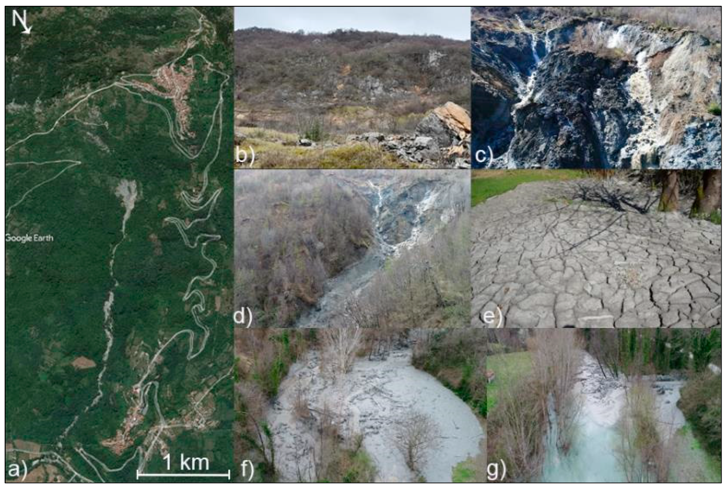
Figure 2.
Geographical location of Morino-Rendinara. Green lines indicate the regional boundaries, red lines indicate the municipality of Morino, Castronovo and San Vincenzo Valle Roveto composing the involved municipality, light blue square indicates the landslide and the study area.
Figure 2.
Geographical location of Morino-Rendinara. Green lines indicate the regional boundaries, red lines indicate the municipality of Morino, Castronovo and San Vincenzo Valle Roveto composing the involved municipality, light blue square indicates the landslide and the study area.
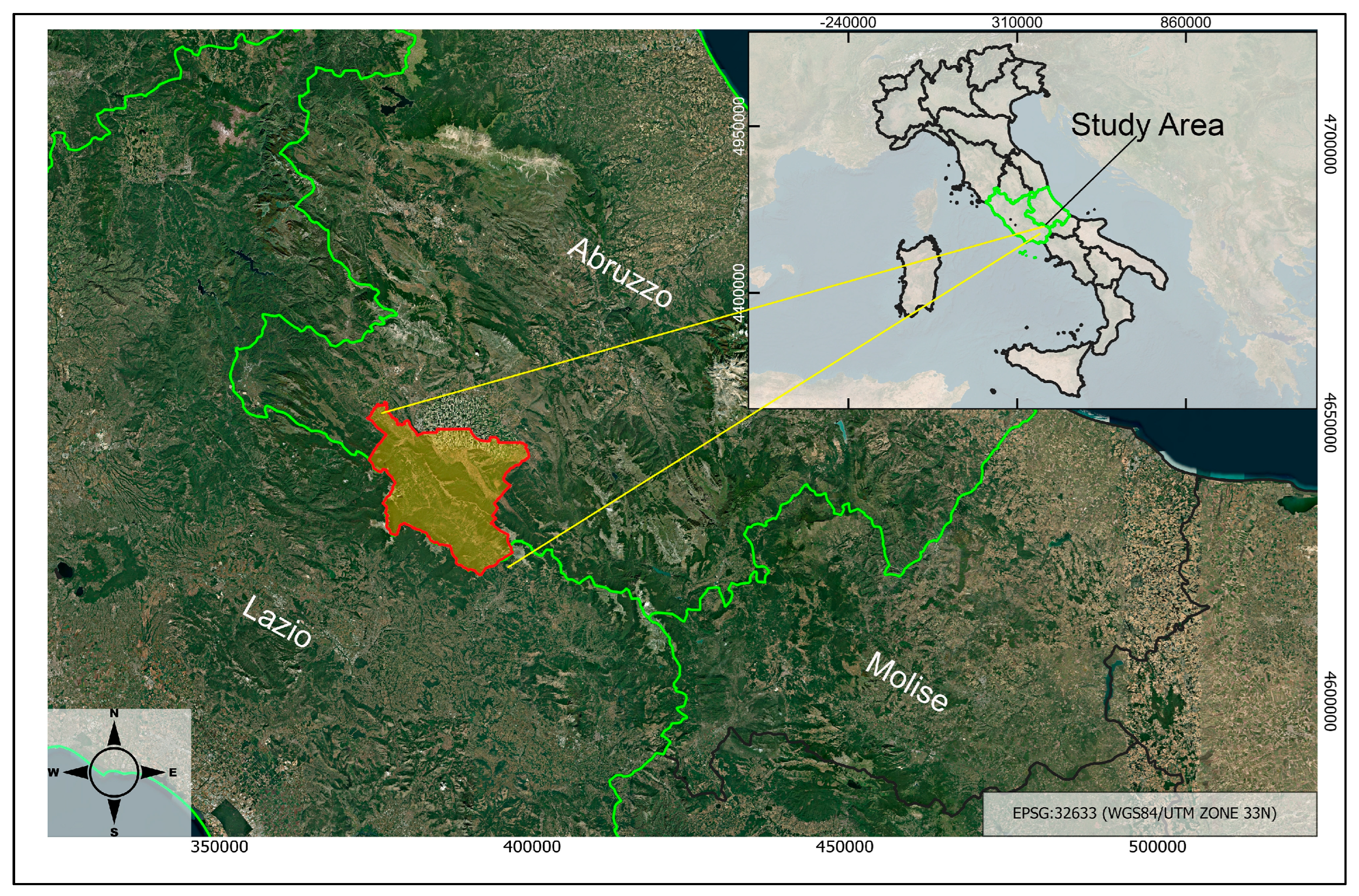
Figure 3.
Geological map of Roveto Valley derived and modified from the Geological Chart 1:100000 Italian CARG Project [22].
Figure 3.
Geological map of Roveto Valley derived and modified from the Geological Chart 1:100000 Italian CARG Project [22].
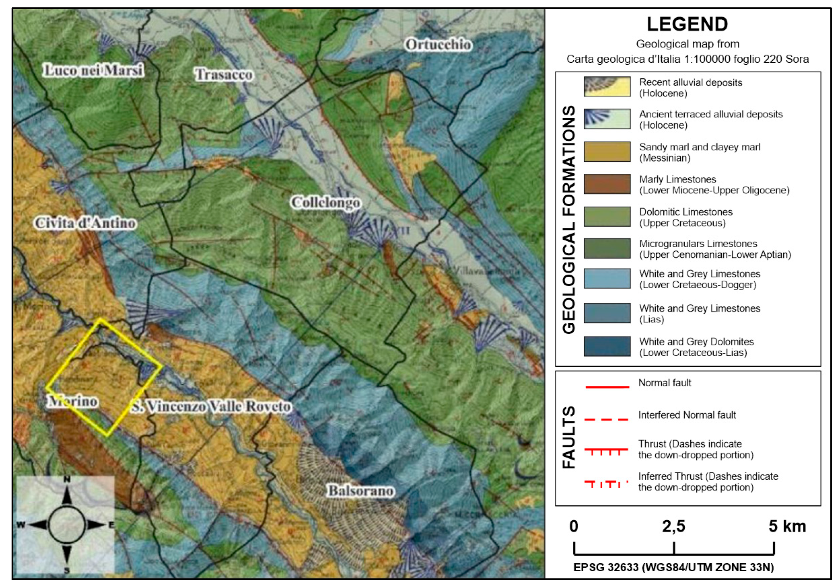
Figure 4.
Maps of the survey and debritic cover layer reconstruction using cross sections to empathize the heterogeneity of deposit covering the substrate.
Figure 4.
Maps of the survey and debritic cover layer reconstruction using cross sections to empathize the heterogeneity of deposit covering the substrate.
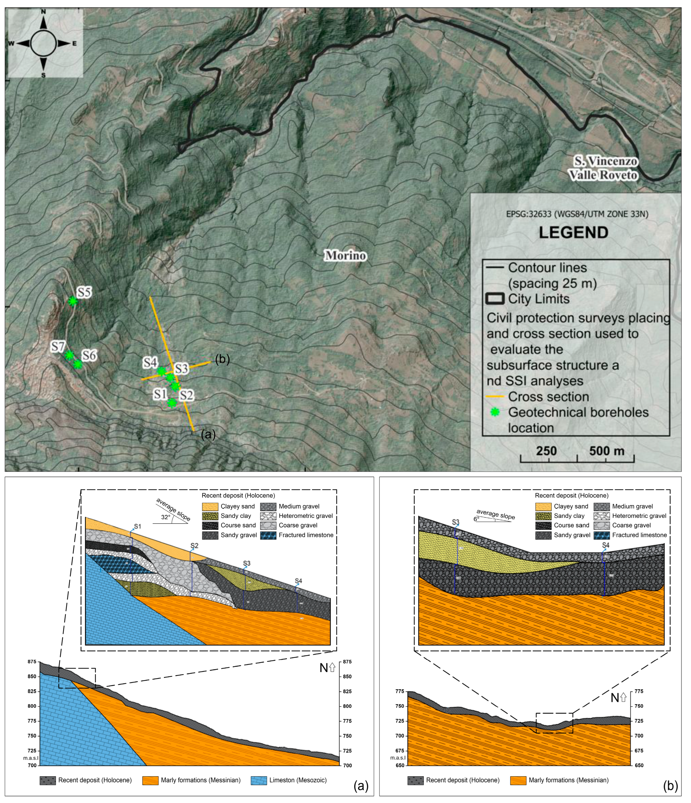
Figure 5.
Conceptual flow chart of the work phases.
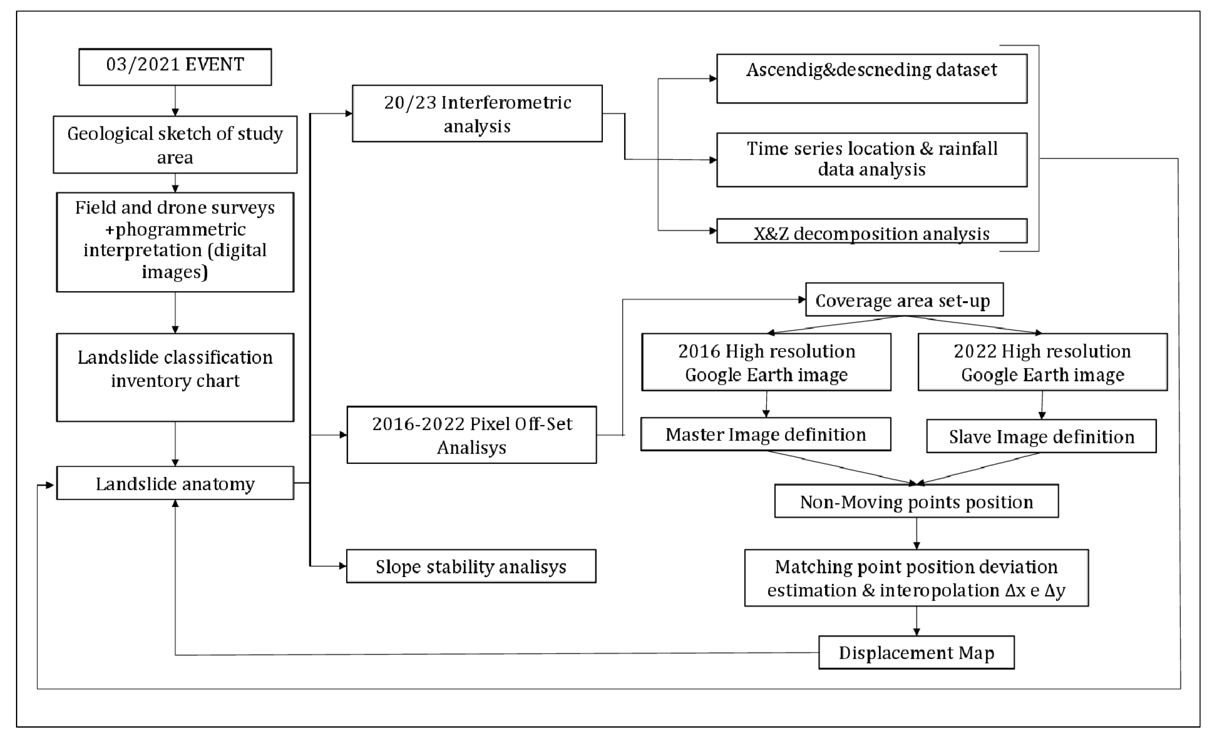
Figure 6.
Landslide inventory map.
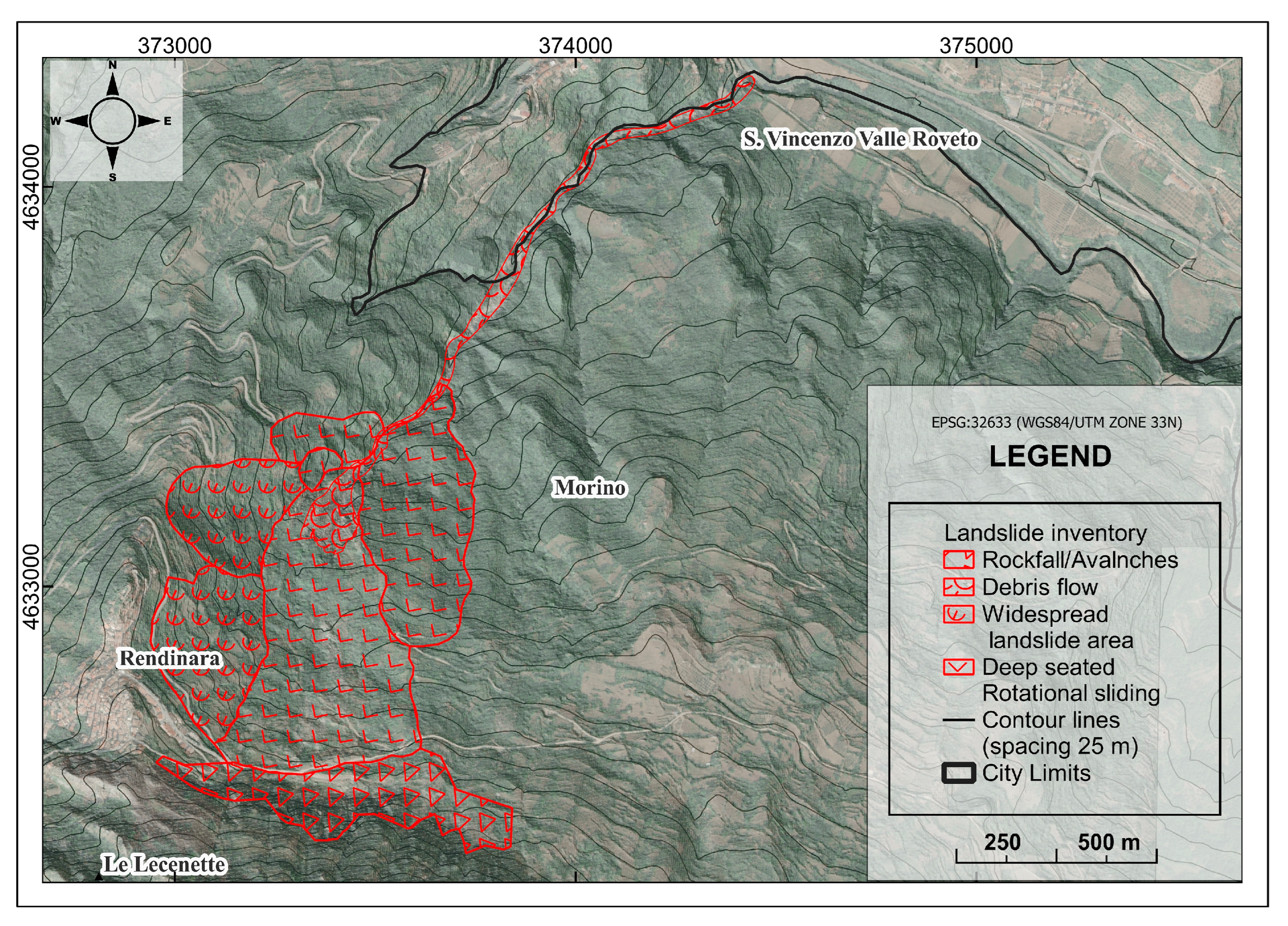
Figure 7.
Pixel offset results red arrows indicate major cumulative displacement along the slope, yellow arrows indicate minor cumulative displacement along the slope.
Figure 7.
Pixel offset results red arrows indicate major cumulative displacement along the slope, yellow arrows indicate minor cumulative displacement along the slope.
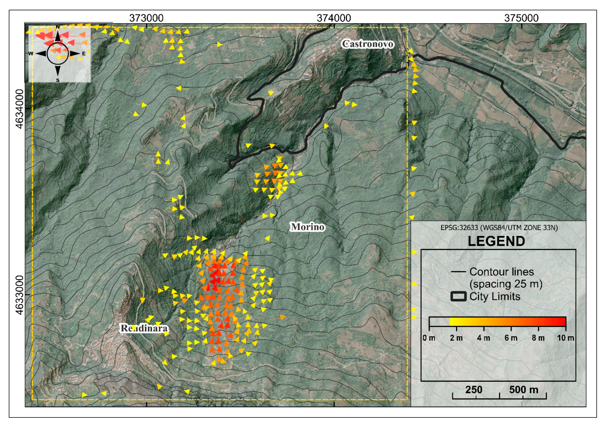
Figure 8.
PS Velocity along the ascending (a) and descending (b) geometry from 2020 to 2023 red dots indicate major velocity trend and instability, green and blue minor velocity, and stable sectors.
Figure 8.
PS Velocity along the ascending (a) and descending (b) geometry from 2020 to 2023 red dots indicate major velocity trend and instability, green and blue minor velocity, and stable sectors.
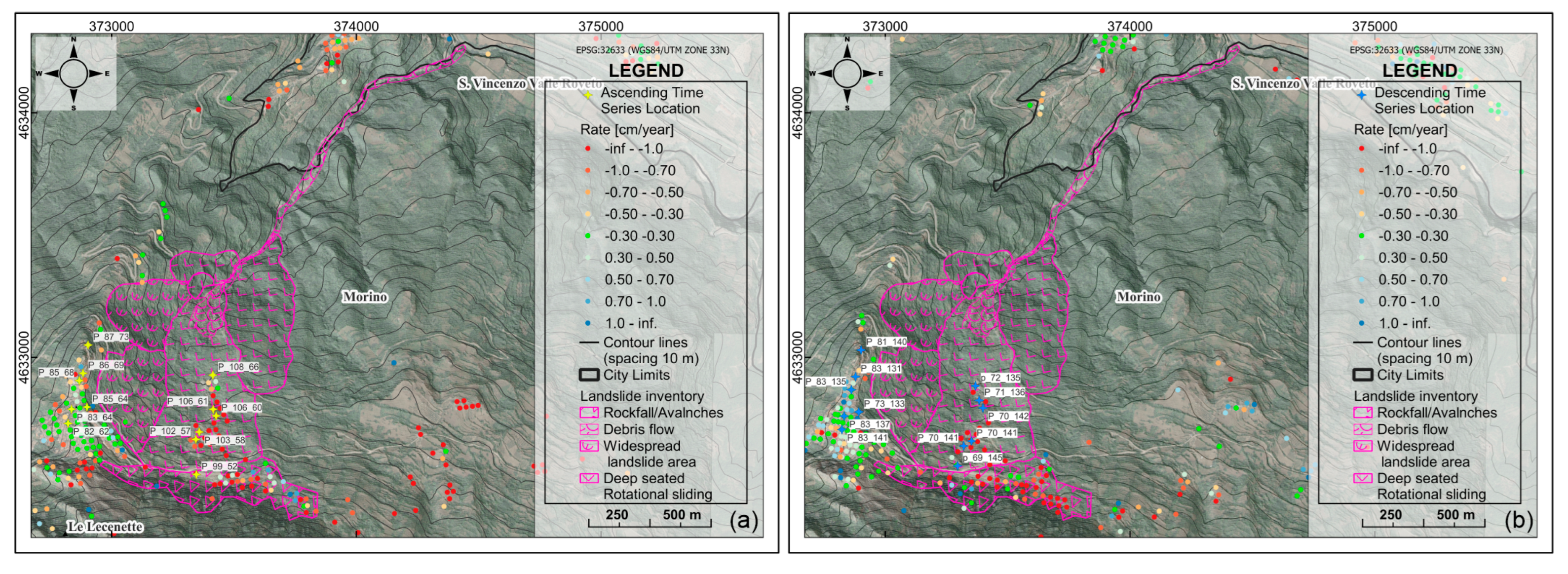
Figure 9.
Selected time series in ascending geometry (a) and descending geometry (b).
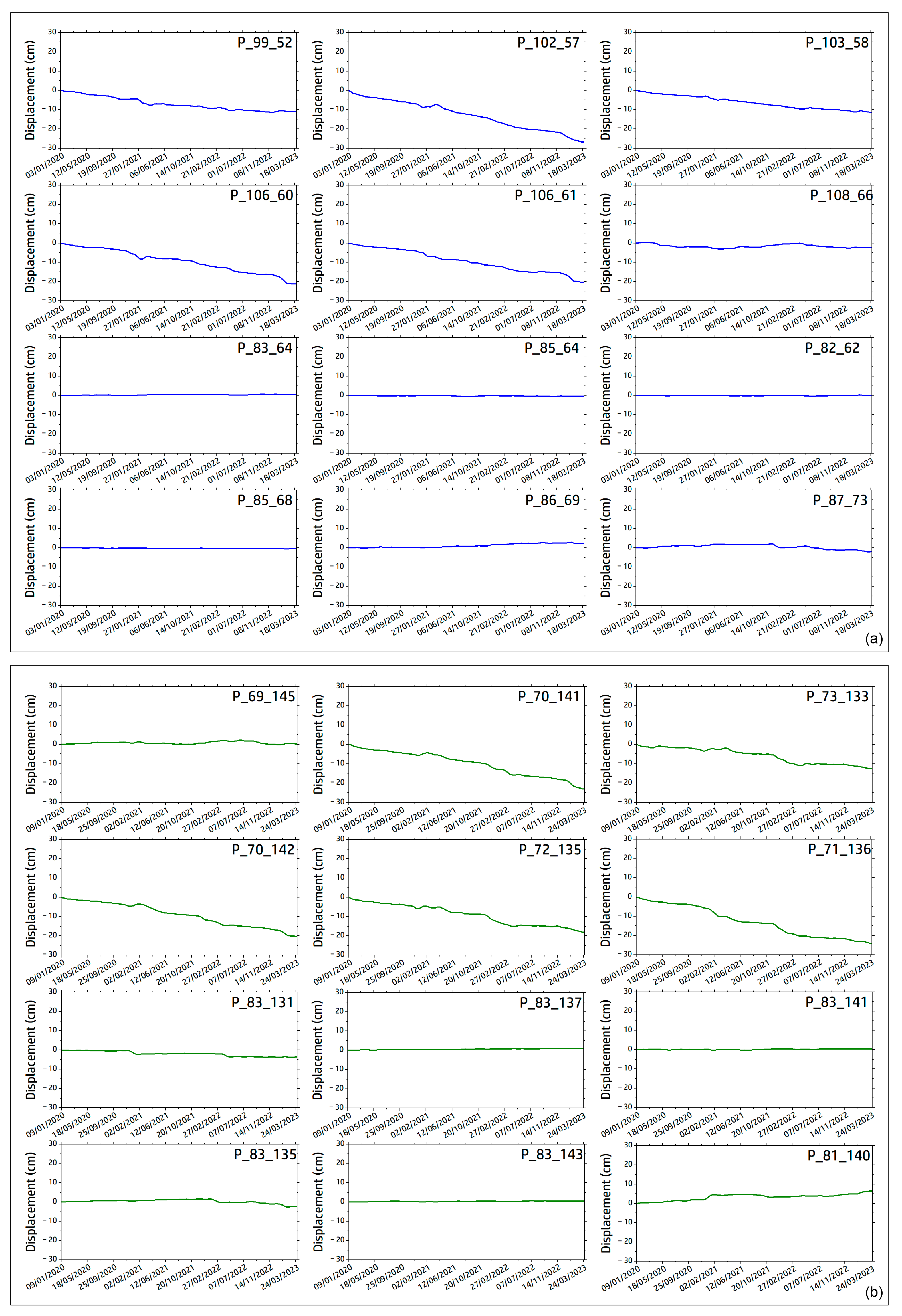
Figure 10.
Time series vs Rainfall analyses. a) Represents monthly cumulative rainfall for analysis period vs one ascending and descending representative time-series, b) Represents daily cumulative rainfall for analysis period vs one ascending and descending representative time-series; c) Represents cumulative rainfall for all analysis period vs one ascending and descending representative time-series.
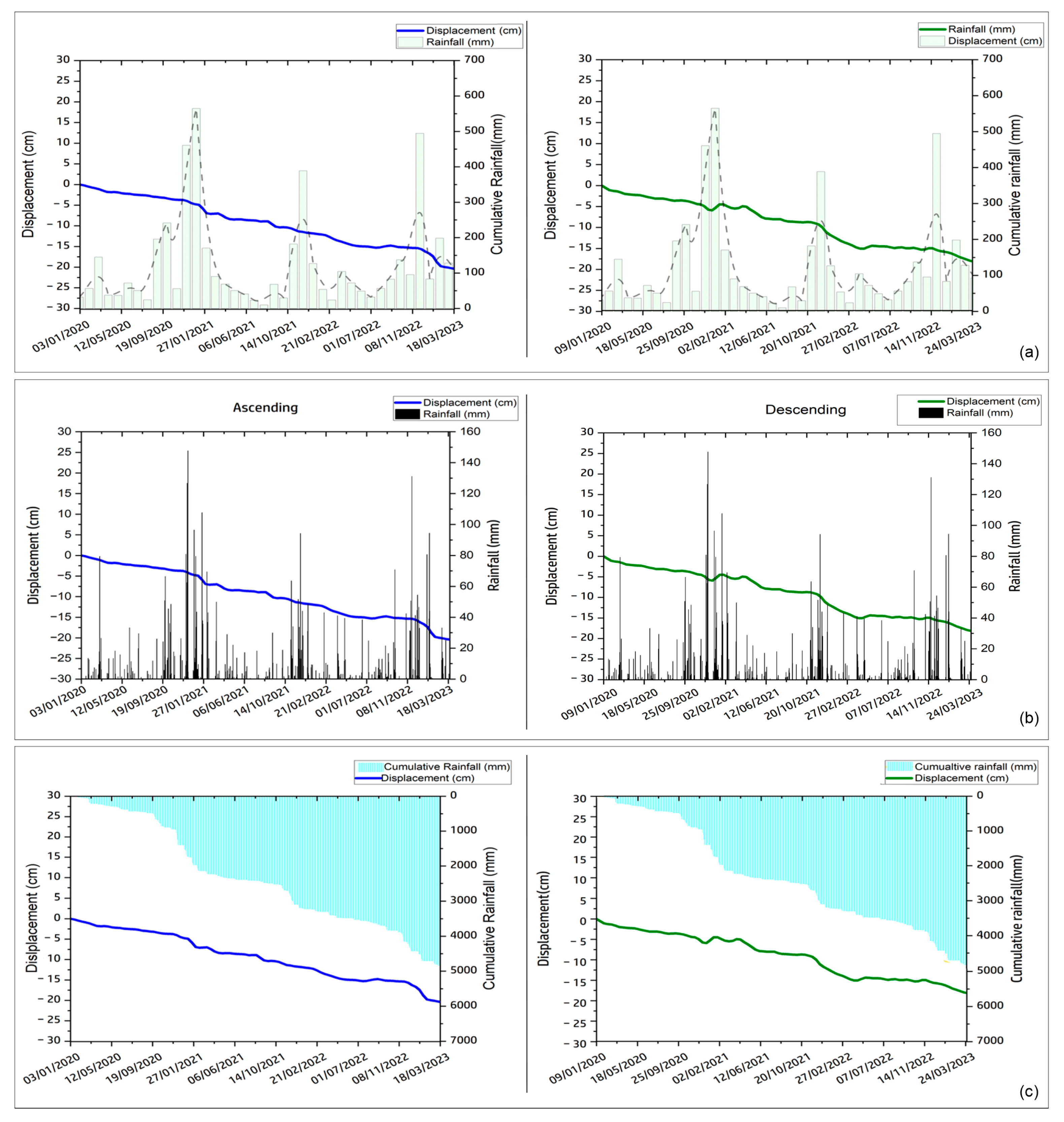
Figure 11.
Adonis software slope stability analyses results, red sector indicates the maximum shear strain along the profile (a, b, c and d). See Figure 5 for the location of the sections.
Figure 11.
Adonis software slope stability analyses results, red sector indicates the maximum shear strain along the profile (a, b, c and d). See Figure 5 for the location of the sections.
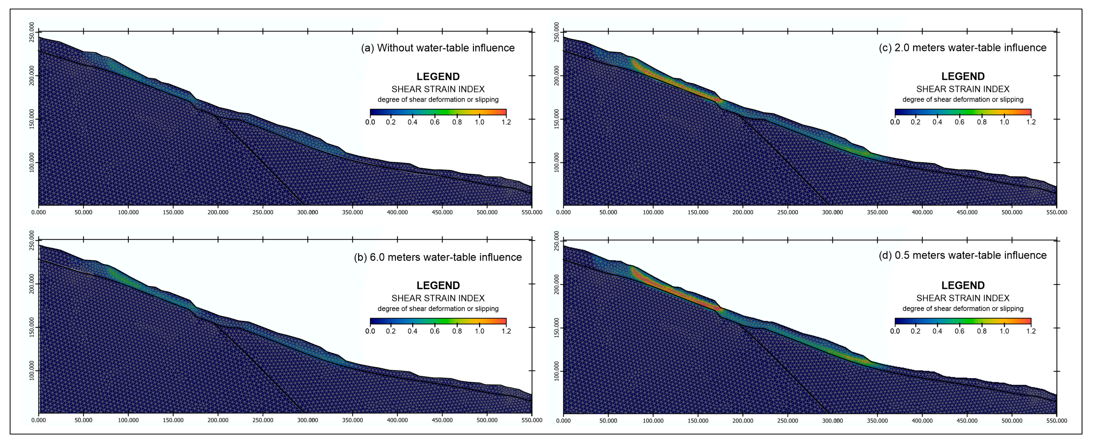

Table 1.
Synthesis the different Cascini formula applied [34].” Yes” indicates presence of corresponding geometry in the grid cell, “No” indicate absence of corresponding geometry in the grid cell. Where and are the velocities obtained from ascending and descending dataset analyses, is the velocity, is the incident angle.
| Ascending | Descending | Applied Formula |
|---|---|---|
| Yes | Yes | |
| Yes | No | |
| No | Yes |
Table 2.
Synthetic table of parameters employed to build the finite element model for slope stability analysis in ADONIS code.
Table 2.
Synthetic table of parameters employed to build the finite element model for slope stability analysis in ADONIS code.
| Parameter | Mesozoic Limestone | Messinian Clay | Cover Layer |
| Unit weight (kg/m3) | 2750 | 2200 | 2300 |
| Young (Pa) | 1.2 e+10 | 3.1+09 | 1.5+09 |
| Poisson | 0.30 | 0.25 | 0.25 |
| Θ( ͦͦ) | - | - | 27 |
| c (Pa) | - | - | 18000 |
| Type | Iso-elastic | Iso-elastic | Mohr Coulomb |
| Shear Modulus (Pa) | 4.61e+09 | 1.24e+09 | 6e+08 |
| Bulk Modulus (Pa) | 1e+10 | 2.06e+09 | 1e+09 |
Disclaimer/Publisher’s Note: The statements, opinions and data contained in all publications are solely those of the individual author(s) and contributor(s) and not of MDPI and/or the editor(s). MDPI and/or the editor(s) disclaim responsibility for any injury to people or property resulting from any ideas, methods, instructions or products referred to in the content. |
© 2024 by the authors. Licensee MDPI, Basel, Switzerland. This article is an open access article distributed under the terms and conditions of the Creative Commons Attribution (CC BY) license (http://creativecommons.org/licenses/by/4.0/).
Copyright: This open access article is published under a Creative Commons CC BY 4.0 license, which permit the free download, distribution, and reuse, provided that the author and preprint are cited in any reuse.


