Submitted:
09 August 2024
Posted:
12 August 2024
You are already at the latest version
Abstract
The monitoring of coastal waters using satellite data, from sensors including Sentinel-3 OLCI, has become a vital tool in the management of these water environments; especially when it comes to improving our understanding of the effects of climate change on these regions. In this study, Level-2 water products derived from different OLCI Sentinel-3 processors were validated against a comprehensive in situ dataset from the NW Baltic Sea proper region. The products validated were those of the regionally adapted Case-2 Regional Coast Colour (C2RCC) OLCI processor (v1.0 and v2.1), as well as the latest standard Level-2 OLCI case 2 (Neural Network) products from Sentinel-3’s processing baseline: Baseline Collection 003 (BC003), including “CHL_NN”, “TSM_NN”, and “ADG443_NN”. Furthermore, the effect of the current EUMETSAT system vicarious calibration (SVC) on the Level-2 water products was also validated. Results showed that the system vicarious calibration (SVC) reduces the reliability of the Level-2 OLCI products. For example, the application of these SVC gains to the OLCI data for the regionally adapted v2.1 C2RCC products resulted in RMSD increases of 36% for “conc_tsm”; 118% for “conc_chl”; 33% for “iop_agelb”; 50% for “iop_adg”; and 10% for “kd_z90max” using a ±3h validation window. The findings indicate that the current EUMETSAT SVC gains should be applied and interpreted with caution in the region of study at present. A key outcome of the paper recommends the development of a regionally specific SVC against AERONET-OC data for the region.
Keywords:
OLCI
; Sentinel-3
; C2RCC
; System Vicarious Calibration (SVC)
; Baltic Sea
; Coloured Dissolved Organic Matter (CDOM)
; Chlorophyll-a
; Total Suspended Matter (TSM)
1. Introduction
In recent decades, remote sensing data has become one of the most important data sources to assess the effect and impacts of climate change [1,2,3,4]. The Global Climate Observing System (GCOS) provides comprehensive observations that are required by the scientific community for monitoring climate change. Furthermore, water-leaving radiance (Lw) derived from satellite data has been designated an Essential Climate Variable (ECV) by GCOS.
Perhaps the most significant development in the field of coastal water remote sensing, was the launch of ENVISATâs Medium Resolution Imaging Spectrometer (MERIS) which operated between 2002 and 2012. MERIS had a spatial resolution of 300m which allowed for coastal waters to be studied at an unprecedent spatial resolution [5,6,7]. However, the launch of the European Space Agencyâs (ESA) Sentinel-3A in February 2016 and Sentinel-3B in April 2018 marked a new era of research and development in ocean colour measurement and monitoring using spaceborne platforms, due to their high spatial resolution and revisit times (1-2 days). Originally developed from MERIS, the two Sentinel-3 satellites house a newly developed ocean colour sensor, the Ocean and Land Colour Instrument (OLCI-A and OLCI-B). The sensor has 21 spectral bands, ranging from 400nm to 1020nm, including dedicated ocean colour bands; these new state-of-the-art optical sensors possess unprecedented spatial, temporal, spectral, and radiometric resolutions for ocean colour satellite monitoring.
However, in order to make water-leaving radiance (Lw) from different ocean colour missions comparable, it must first be calibrated against high quality in situ data [8]. This process is termed: system vicarious calibration (SVC), and it is undertaken by applying SVC gains to the water-leaving radiance (Lw). As noted by [9], SVC for ocean colour applications was first introduced by Gordon et al. [10], who recognised the requirement for such optical sensors to be precisely calibrated to accurately measure the often minute water-leaving radiance (Lw) signal. These gains are defined as the ratio between the expected (measured in situ) and actual top of atmosphere (TOA) radiances, at each wavelength band, received at the satellite sensor [9]. A correction, which represents the difference between the radiances observed in situ and those observed from the satellite sensor, termed the SVC gains, is applied to the satellite radiances such that they precisely match the in situ optical measurements [9]. In theory, this correction should improve the satellite radiance product; however, SVC gains differ between water regions, and therefore, the SVC gains EUMETSAT currently provide for Sentinel-3 OLCI-A and OLCI-B [11] effectively represent an average of SVC gains from their respective in situ measurement sites. These average gains are recalculated on an ongoing basis as new matchups (correspondence between in situ and TOA reflectance) are obtained over the lifetime of the mission. The SVC of OLCI data is based on the gains from the Marine Optical BuoY (MOBY) off the coast of Hawaii, which has also been used for SVC of various ocean colour satellites operated by NASA (such as SeaWiFS and MODIS; [12]). Usually, SVC gains are applied during pre-launch, as well as post-launch (on-orbit) radiometric calibration [13], with the aim to retrieve a satellite-derived water-leaving radiance (Lw) within a spectrally independent uncertainty of 5% [8]. While SVC has always been applied to MODIS data, it has been implemented on OLCI-A data since June 2017, which means data from both missions are now comparable ([14]). While the SVC is widely considered a requirement for adequate merging of multi mission ocean colour data, it is not clear if the derived gains applied to OLCI Sentinel-3 data are applicable for all types of optically complex waters, for example in the Baltic Sea. The analysis by [15,16] showed that the results of the locally adapted processor (which did not include SVC gains) returned better results than the processor which used SVC. This was to be expected for the Total Suspended Matter (TSM) product, as a regional parameterisation of the specific scatter had been applied according to [17]. However, it is unlikely that the positive effect on the other water products was due solely to the local adaptation of the salinity and temperature parameters in the processor. However, the effect of the SVC gains on OLCI derived Level-2 water quality products for the Baltic Sea region has not been widely examined. While [16] found that the current SVC applied to OLCI Sentinel-3 data is not beneficial for the retrieval of Baltic Sea water products, the effect of SVC was not quantified in their study.
Due to the extensive body of research and in situ ground truth data available for the region, the Baltic Sea serves as the ideal case study for evaluating the use of remote sensing for coastal water quality monitoring. Additionally, this region represents one of the most optically complex sea waters globally, with a predominant Coloured Dissolved Organic Matter (CDOM) influence on the spectral absorption and reflectance signature [6,17,18,19,20] which is accompanied with relatively low particle scatter (Figure 6). Kirk [21] noted the Baltic Sea’s relatively high CDOM concentration for a marine waterbody and the decreasing CDOM concentrations from the Bothnian Gulf southwards in relation to the proportion of river water in the marine water.
Here, we undertake a validation of the latest satellite-based water products for Chlorophyll-a (Chl-a), TSM, CDOM, and Secchi depth. A matchup analysis was undertaken between the latest Sentinel-3 OLCI-A and OLCI-B water quality products and newly aggregated in situ water quality data for the Baltic Sea region. Several products and processing schemes were assessed, and a comparison was undertaken to evaluate which performed favourably in the region. By combining in situ datasets from previous Sentinel-3 OLCI validation studies, such as [15,16], as well as newly available in situ data from the Swedish national pelagic monitoring program (funded by the Swedish Agency for Marine and Water Management, SwAM), one of the most comprehensive validation datasets for Sentinel-3 OLCI water products in the western Baltic proper region to date was created. The objectives of the research were to: 1) validate the latest OLCI Level-2 water products in the region; 2) to assess the current EUMETSAT OLCI SVC gains on the Level-2 water products for the region; and, 3) to assess the effects of changes in the Case-2 Regional Coast Colour (C2RCC) processor between v1.0 and v2.1, especially the revised TSM equation in v2.1, on the Level-2 water products for the region.
2. Materials and Methods
After the application of data quality flags and the respective matchup time windows, matchup datasets ranging between n=29 and n=171 were obtained for the different OLCI-based water products. These satellite/in situ matchup data pairs were used to validate: 1) the latest products of the Neural Network-based C2RCC processor; 2) the latest EUMETSAT SVC gains; and 3) the latest EUMETSAT Level-2 OLCI standard NN products. The C2RCC OLCI outputs âconc_chlâ, âconc_tsmâ, âiop_agelbâ and âiop_adgâ, as well as âkd_z90maxâ (from both C2RCC v1.0 and v2.1) were validated against their respective in situ measurements. The âiop_agelbâ and âiop_adgâ products are both proxies for CDOM, while âkd_z90maxâ is a proxy for Secchi depth. The C2RCC OLCI-based water quality products were processed in three ways: 1) Sentinel-3 OLCI C2RCC v1.0 without SVC; 2) Sentinel- 3 OLCI C2RCC v2.1 without SVC; and 3) Sentinel-3 OLCI C2RCC v2.1 with SVC applied. This is the first time the effects of the latest EUMETSAT SVC gains on the retrieval of OLCI Level-2 water products has been validated in the study region. Additionally, some of the EUMETSAT Level-2 standard water products from the Baseline Collection 003 (BC003) were also validated for the region; âCHL_NNâ, âTSM_NNâ, and âADG443_NNâ.
2.1. Region of Interest (ROI)
The Region of Interest (ROI), which includes the coastal waters of Svealand, is illustrated in Figure 1. This ROI represents a coastal optical Case 2 water environment, with in situ validation sampling stations spanning approximately 300km along the east coast of Sweden, in the NW Baltic proper region.
2.2. Matchup Data
Two types of data are required to perform a satellite-based matchup analysis; 1) extensive in situ validation data is required to ensure that enough in situ samples can be temporally and spatially matched to the satellite data; and 2) satellite data which is spatially and temporally coincident with at least some of the in situ data points. The following sections discuss the acquisition, matchup, and processing of both the in situ validation data and satellite data used in this study.
2.2.1. Validation Data
As part of this study, we aggregated in situ water quality datasets from three sources to create an extensive validation dataset of water quality products for the Baltic Sea proper region. These three in situ datasets, collected between May 2016 and August 2022, comprise of boat-based discrete water samples for the four optically active constituents, these are: TSM (g m-3), Chl-a (µg L-1), CDOM absorption (m-1), and Secchi depth (m). The three datasets from which the new aggregated dataset was created were:
Chl-a was measured spectrophotometrically using the trichromatic method [26,27]. The samples from MG were extracted in ethanol, while those from Kyryliuk and Kratzer [15] and Kratzer and Plowey [16], provided by the Marine Remote Sensing Group (MRSG) at Stockholm University, were extracted in acetone. The samples from the two laboratories have been shown to lie within 5% difference in several intercomparisons of methods [28]. TSM was measured gravimetrically, following the method detailed in [29] and the MERIS protocols [30], while turbidity was measured as outlined in [31]. Finally, CDOM was measured spectrophotometrically using the method described in [6].
The validation samples for Chl-a concentration ranged from 1.02 to 28.58µg L-1; TSM concentration ranged from 0.28 to 6.57g m-3; the absorption of CDOM at 440nm (aCDOM) ranged from 0.28 to 1.4 m-1; and Secchi depth measurements ranged from 3 to 11 meters. All Secchi depth measurements were captured with the use of a water telescope, which improved the validation results in tests. Additionally, all water samples were surface samples, captured within approximately <1 meter depth from the waterâs surface and at stations which have a depth greater than that which would be subject to the bottom effect. In the absence of TSM data, and where turbidity data was available, turbidity (FNU) was converted to TSM (g m-3) according to the algorithm derived by Kari [31] for the region, shown in Equation 1; this increased the number of TSM validation samples available for use in this study.
Where: TSM = TSM concentration (g m-3) and t = turbidity (FNU).
The three in situ datasets were combined and cleaned, with duplicate, incomplete, or missing samples removed. This cleaned dataset was then used to find spatio-temporal coincident matchup Sentinel-3 OLCI-A and OLCI-B products for the matchup analysis/validation. In keeping with the validation time windows used in previous studies in the region [7,15] the matchup analysis was undertaken using samples collected within both a ±2h and ±3h time window of the Sentinel-3 overpasses. These matchup time windows consider the coastal dynamics and thus the rate of change of the optical in-water conditions over time in the region [15,32]. Due to the 300m spatial resolution of OLCI-A and OLCI-B, there was a possibility of near-land pixels to be mixed pixels of both land and water signals. Therefore, samples within <424 meters distance from land were identified and removed from the validation dataset, as this distance represents the diagonal length of a Sentinel-3 OLCI pixel (300m x 300m square pixel), to ensure that the respective pixel does not overlap with land. Additionally, this 424m threshold also sought to reduce adjacency effects from land.
From the initial 2,940 in situ samples, the resultant aggregated and cleaned matchup datasets contained 407 and 558 in situ samples coincident with the Level-1 satellite data, as well as 256 and 357 samples coincident with the Level-2 standard products, for the ±2h and ±3h time windows respectively. However, this number was reduced in the final validation due to the application of the OLCI data quality flags, as seen in the N values shown in Section 3 and Table 1. This was largely due to the high percentage of cloud cover observed for the Baltic Sea region [15,17,33,34], which meant that only a fraction of the in situ validation data was suitable for the validation of satellite products.
2.2.2. Satellite Data
Due to the coastal nature of the ROI, a 1x1 pixel validation window was used. Normally, it is recommended that a 3x3 aggregated macropixel window is used for the validation of Sentinel-3 OLCI satellite products; however, this is not always possible for near-coast regions where a limited number of pixels are available, and therefore a 1x1 pixel window can be used for match-up analysis in such environments [15,35].
2.2.2.1. Level-1 S3 EFR OLCI Data
Sentinel-3 Level-1 EFR OLCI products, from Baseline Collection 002 (BC002), were identified using SentinelSat API [36] which queried the Copernicus Open Access Hub [37] API using the in situ sample dates, times, and coordinates for each sample in the in situ dataset to find matchup Sentinel-3 OLCI A and OLCI-B products. However, the Copernicus Open Access Hub has since been closed, and all products are currently available from the Copernicus Data Space Ecosystem [38]. Cloud masks were not used, which ensured all possible matchup products were identified. After the initial matchup, the validation time window was then narrowed to ±2h and ±3h respectively, data quality flags were applied (see Section 2.2.2.3), and the resultant OLCI products were utilized to validate the processing chains.
Table 1 summarizes the number of Level-1 OLCI products and corresponding validation samples for each of the processing chains and validation time windows evaluated, before and after the application of the OLCI data quality flags. By default, no SVC gains were applied to this Level-1 OLCI-A and OLCI-B data at source. Supplementary Tables S.1 to S.6 (see Supplementary file) show the final Level-1 EFR OLCI matchup products used for each of the three individual C2RCC processing chains, identified in Table 1, for both the ±2h and ±3h validation windows. Figure 2 below shows an overview of the full C2RCC processing and validation workflow for both the SVC and non-SVC Level-1 OLCI products.

Table 1.
Number of matchup products and samples for each OLCI product before and after the application of OLCI data Quality Flags.
Table 1.
Number of matchup products and samples for each OLCI product before and after the application of OLCI data Quality Flags.
| OLCI Product | Time Window | No. OLCI Matchup Products | No. Matchup Samples | |
|---|---|---|---|---|
| Before Data Quality Flags | ||||
| OLCI Level-1 | +/- 2hr | 180 | 407 | |
| +/- 3hr | 190 | 558 | ||
| OLCI Level-2 | +/- 2hr | 102 | 256 | |
| +/- 3hr | 109 | 357 | ||
| After Data Quality Flags | ||||
| C2RCC v1.0 (OLCI Level-1) | +/- 2hr | 70 | 135 | |
| +/- 3hr | 82 | 180 | ||
| C2RCC v2.1 (OLCI Level-1) | +/- 2hr | 70 | 127 | |
| +/- 3hr | 86 | 170 | ||
| C2RCC v2.1 (OLCI Level-1) SVC | +/- 2hr | 72 | 131 | |
| +/- 3hr | 86 | 172 | ||
| EUMETSAT Level-2 (OLCI Level-2) | +/- 2hr | 80 | 133 | |
| +/- 3hr | 96 | 181 |
2.2.2.2. Level-2 S3 WFR OLCI Data
The Level-2 Sentinel-3 OLCI-A and OLCI-B WFR products, from Baseline Collection 003 (BC003), were downloaded directly from the EUMETSAT Data Store [39]. As the matchup OLCI products were already identified by the Python script for the Level-1 OLCI products; another matchup was not necessary. These Level-2 OLCI products include the three EUMETSAT standard water quality products: 1.) âCHL_NNâ, 2.) âTSM_NNâ, and 3.) âADG443_NNâ, which were validated. Table 1 shows the number of OLCI Level-2 products and corresponding validation samples for the EUMETSAT standard product processing chain for both the ±2h and ±3h validation time windows, before and after the application of the OLCI data quality flags. By default, SVC gains are applied to these Level-2 water products at source. Supplementary Tables S.7 and S.8 (see Supplementary file) show the final EUMETSAT Level-2 OLCI products used for the validation. As these are already Level-2 products, the validation processing chain was straightforward, as illustrated in the validation workflow diagram Figure 3.
2.2.2.3. OLCI Data Quality Flags
Sentinel-3 OLCI data quality flags were used to exclude problematic OLCI pixels from the validation, including cloud, land, and sun glint pixels, for example. The data quality flags used were informed by those used in the works of: [15,16,40]. These data quality flags were applied in the âPix Ext and Data Quality Flagsâ step illustrated in the workflow diagrams: Figure 2 and Figure 3.
Two types of data quality flags are used in this study: 1) the standard OLCI product data quality flags; and 2) the C2RCC data quality flags. For the Level-1 OLCI data, the data quality flags used by [15], highlighted in grey in Table 2, were used as the baseline data quality flags. Additional data quality flags identified by [16,40], also listed in Table 2, were evaluated individually using a Python script to find which data quality flags improved the validation results Pearsonâs r value. It was found that of the flags evaluated, only the addition of one extra data quality flag (to the baseline quality flag expression), the âquality_flags.sun_glint_riskâ flag, improved the validation results, with the remainder having almost no effect on the Pearson r value. Therefore, this data quality flag was added to the baseline quality flag expression, as illustrated in Table 2. The results of the data quality flag tests can be found in Supplementary Tables S.11 and S.12 (see Supplementary file). As noted, the application of data quality flags substantially reduced the number of suitable matchup products and in situ validation samples, as can be seen in Table 1. For the EUMETSAT Level-2 OLCI products, the EUMETSAT recommended data quality flags were applied [11], as shown in Table 3.
2.3. System Vicarious Calibration (SVC)
In this study, the effects of the current EUMETSAT SVC gains on these OLCI water products is validated for the region by applying these gains to the Level-1 OLCI radiance data prior to processing in C2RCC, and comparing the validation results to those where no SVC gains was applied. The latest EUMETSAT SVC gains [11] are graphed in Figure 4 and Figure 5, and can also be found in Supplementary Tables S.9 and S.10 (see Supplementary file). These SVC gains were applied to each Level-1 OLCI-A and OLCI-B radiance band by multiplying the band values of each pixel by the appropriate SVC gain value.
2.4. Case 2 Regional CoastColour (C2RCC)
The C2RCC processor is based on a machine learning (ML) neural network (NN) approach. The processor includes an atmospheric correction (AC) model which is coupled with a bio-optical model based on Hydrolight (Numerical Optics Ltd., UK), including several semi-analytical inherent optical properties (IOP) algorithms. Originating from [41,42], the Case-2 Regional processor (C2R) draws on a vast library of global IOP data to simulate an extensive range of optical water conditions sensed remotely over Case 2 waters (forward model). A vast library of IOPs with coinciding reflectance spectra is used to train the C2RCC NN. Subsequently, the water products (IOPs) are derived from the remote sensing reflectance via inverse modelling in an iterative way until the measured and simulated spectra match. Intermediate results are the scatter (b), as well as the absorption (a) at 442 nm. Using semi-analytical relationships, TSM is derived from b442, while both the Chl-a concentration and the CDOM absorption are derived from a442. The products can be regionally adapted by, e.g., applying a mathematical relationship between the regionally specific IOP and the related water product, for example the TSM-specific scatter, and the TSM concentration. Initially, the C2R processor was trained on data from the North Sea [41] and has been tested successfully in the Baltic Sea [6,43].
Over time, the processor was further developed â using training data from other coastal waters - and renamed the Case 2 Regional CoastColour (C2RCC) [44]. The C2RCC processor is designed for use with Landsat-8 OLI, Sentinel-2 MSI, Sentinel-3 OLCI, MERIS, MODIS, VIIRS, and Sea WiFS. It is currently available as a Graphical User Interface (GUI) through SNAP, as a CLI, and through Python using the SNAP Python tool: SNAPPY. In this work, the current version of C2RCC (v2.1), as well as the older C2RCC v1.0, was used through SNAP Version 9 and Version 6 respectively through Python scripts using SNAPPY and the CLI to automate the processing. SNAP 10 has since been released, however the current version of C2RCC is still v2.1. The C2RCC OLCI processor outputs numerous Level-2 products, all of which are listed in Table 4 along with a description of each.
2.4.1. C2RCC Parameterisation
This section describes the parameterisation of the regionally adapted C2RCC OLCI processor, largely based on the work of Kyryliuk and Kratzer [15]. However, some of these parameters were modified and updated for the latest version of the C2RCC processor (v2.1). Depending on the season, two different water temperature parameters were used [15]. For the months of April, May, and October 5°C was used, and for June, July, August, and September 15°C was used (C2RCC Default). Salinity was approximated at 6.5 PSU for the region; however, temperature and salinity values only have a minor influence on the results of the C2RCC processor [16]. The C2RCC v1.0 processing chain, termed: âv1.0 Reg Adapâ, used the same parameters as Kyryliuk and Kratzer [15], apart from the salinity, which was set to 6.5 instead of 7 used in the preceding study, as shown in Table 5.
Due to changes made between v1.0 and v2.1 of C2RCC, relating to how âconc_tsmâ was calculated, a different TSM parameterisation was applied between the two versions. The equation used to relate the in situ concentration of TSM to both the marine and white particle scatter at 443nm (âiop_bpartâ and âiop_bwitâ) was changed from a linear equation in v1.0 (Equation (2)) to an exponential equation in v2.1 (Equation (3)). It was also observed that the âiop_bpartâ and âiop_bwitâ outputs between v1.0 and v2.1 were notably different, meaning that the TSM equations were only compatible with their own version of the processor and not interchangeable between v1.0 and v2.1.
Where bpart is the C2RCC âiop_bpartâ product and TSMfakBpart is its corresponding factor; bwit is the C2RCC âiop_bwitâ product and TSMfakBwit is its corresponding factor.
Where TSMfac is the TSM factor, iop_btot is the C2RCC âiop_btotâ product, and TSMexp is the TSM exponent.
Additionally, the default values changed for âThreshold rtosa OOSâ and âThreshold AC reflectances OOSâ between v1.0 and v2.1 of the processor, as shown in Table 5.
For C2RCC v1.0, the âTSM factor bpartâ represents the inverse of the SPM-specific scatter in the Baltic Sea region [45], represented in Equation (4). Kratzer and Moore [17] calculated a mean SPM-Specific Scatter for the Baltic Sea ROI as: 1.016 (±0.326 m2 g-1) (n = 56), resulting in a multiplicative inverse value of ~0.986 for âTSM factor bpartâ; this is the value Kyryliuk and Kratzer [15] used, and as such, is the value used in C2RCC v1.0 in this study. As also informed by [15], a âTSM factor bwitâ value of 1.72 was used.
Where = SPM-specific scatter.
For the first C2RCC v2.1 processing chain, termed: âv2.1 Defâ, the default TSM parameter values for the âTSM factorâ and âTSM exponentâ were used, as listed in Table 5. Following this, regionally adapted âTSM factorâ and âTSM exponentâ values were used in the âv2.1 Reg Adapâ processing chain, also shown in Table 5. These regionally adapted parameters were calculated using in situ particle backscatter (bpart) and corresponding TSM concentration (g m-3) data for the Baltic Sea region collected by [17]. This bpart data was plotted against aCDOM (m-1) in Figure 6 (see Section 3). As shown in Equations (2) and (3), the variables âiop_bpartâ and âiop_bwitâ in the C2RCC v1.0 equation have been replaced in the v2.1 equation with a single variable representing the total scatter, âiop_btotâ. This represents the total particle scatter of both marine particles and white particles (whitecaps) at 443nm (iop_btot = iop_bpart + iop_bwit), as shown in Table 4. Using the in situ marine particle backscatter data (bpart), and assuming a white particle backscatter (bwit) of 0 for the region, total particle backscatter (btot) was calculated as shown in Equation (5).
Where it was assumed that in_situ_bwit = 0, as white caps are rarely observed in the Baltic Sea (unless during a storm).
The resultant in_situ_btot data was used with the corresponding in situ TSM concentration (g m-3) data to calculate the optimal values for both the âTSM factorâ and âTSM exponentâ parameters for âv2.1 Reg Adapâ. The Generalized Reduced Gradient (GRG) solver method was used to vary the parameter values in Equation (3) to find the optimal values for the two parameters. This was done by minimizing the sum of the squared residuals (SSR) between the output âconc_tsmâ and the in situ TSM concentration. The final TSM parameter values derived was a âTSM factorâ of 1.212 and a âTSM exponentâ of 0.686, with a final SSR value of: 86. This showed an improvement over the default âTSM factorâ and âTSM exponentâ values which returned an SSR of 238 when evaluated on the same data for the region. It was also observed that varying the C2RCC TSM parameter values does not affect the other outputs validated (âconc_chlâ, âiop_agelbâ, âiop_adgâ, and âkd_z90maxâ). The final parameters used in each of the C2RCC v1.0 and v2.1 processing chains can be seen in Table 5.
2.4.2. Validation Difference Metrics
Equations (6), (7), (8) and (9) show the difference metrics used to assess the performance of each processor/processing chain [6,46]. These include Pearson’s correlation coefficient (r), Mean Normalised Bias % (MNB), Root Mean Square Difference % (RMSD), and Mean Absolute Percentage Difference % (MAPD).
3. Results
Figure 6 below shows the relationship between CDOM absorption (aCDOM) and particle scatter (bpart) at 440nm for the Baltic Sea, North Sea, English Channel, and the Adriatic Sea. As can be seen, this relationship is very different in the Baltic Sea compared to the other European Seas. For the same bpart at 440nm values, the Baltic Seaâs aCDOM (m-1) values were found to be much higher than those of the North Sea, English Channel, and Adriatic Sea.
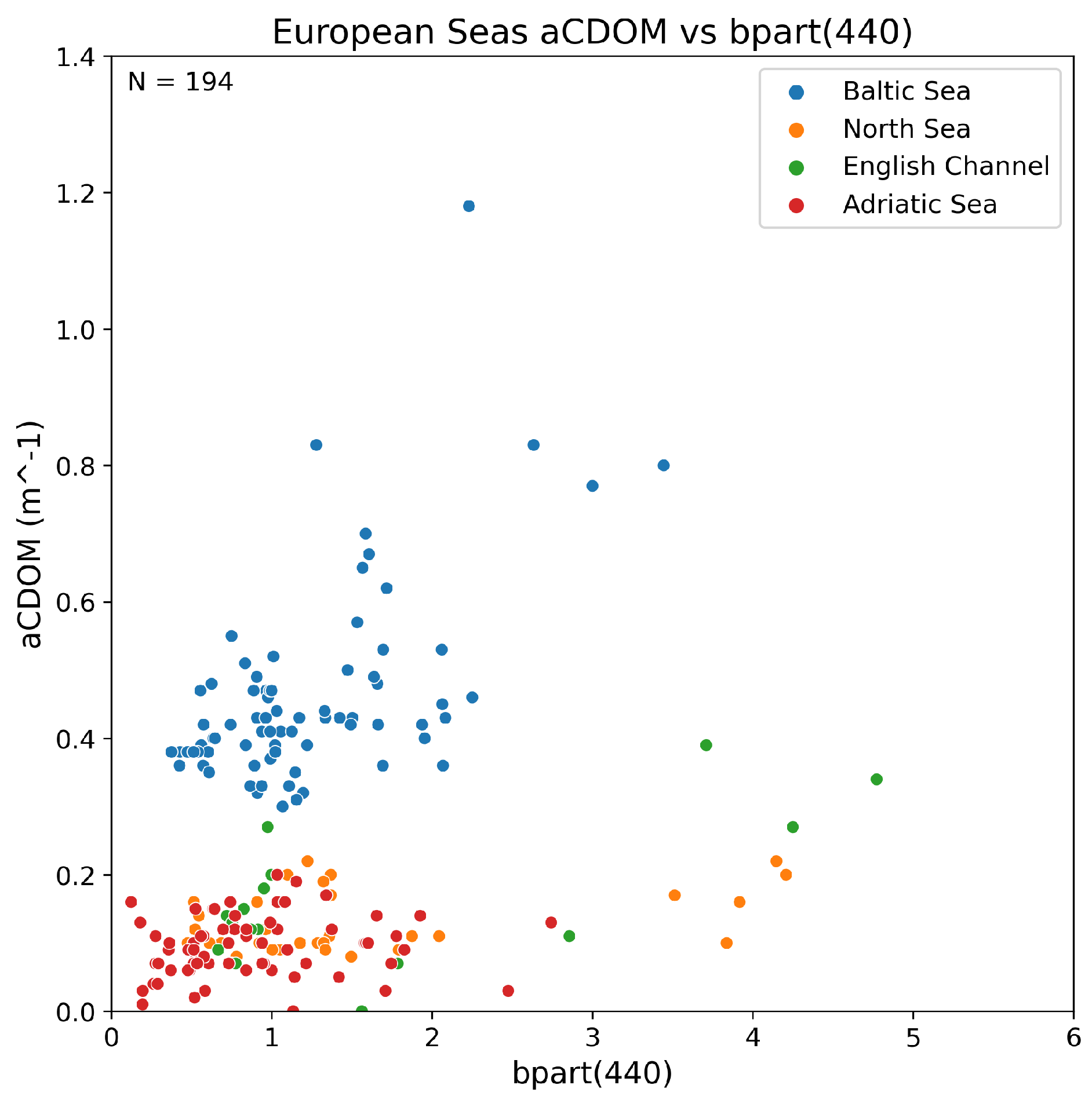
Figure 6.
CDOM absorption (m-1) vs. bpart(440), showing the relatively high CDOM absorption observed in comparison to particle backscatter at 440nm (bpart(440)) in the Baltic Sea region when compared to other European Seas. Baltic Sea data from [17]. North Sea, English Channel, and Adriatic Sea data was obtained from the COLORS project [47].
Table 6 shows the C2RCC âconc_tsmâ validation results for each of the processing chains tested (both the ±2h and ±3h time windows); the SVC results are highlighted in the grey columns. The first column shows the regionally adapted v1.0 productâs validation results, which performed best for MNB, RMSD, and MAPD by a large margin. Although the v2.1 C2RCC products did perform best for Pearsonâs r, this was accompanied by poor % MNB, RMSD, and MAPD values. Additionally, both SVC processing chains performed poorly when compared to the other processing chains validated. These key findings are discussed in greater detail in Section 4.
Table 7 summarises the âconc_chlâ, âiop_agelbâ, âiop_adgâ and âkd_z90maxâ C2RCC validation results for each of the processing chains, for both the ±2h and ±3h time windows. Like the âconc_tsmâ results, the application of SVC did not improve the productâs overall validation performance, as shown in the grey columns. Both the âconc_chlâ and âkd_z90maxâ products performed best in C2RCC v1.0, while the CDOM productâs (âiop_agelbâ, âiop_adgâ) performance was more closely matched between the two versions. As noted, the key findings are discussed in full in Section 4 below.
Table 8 below summarises the validation results for the EUMETSAT Sentinel-3 OLCI Level-2 NN standard (non-regionally adapted) products; âTSM_NNâ, âCHL_NNâ, and âADG443_NNâ. These three standard products were outperformed by the regionally adapted C2RCC products, showing lower Pearson R values, and higher % MNB, RMSD, and MAPD values; this comparison will be discussed detail in Section 4 below.
4. Discussion
This section reviews the results presented in the previous section; beginning with the non-SVC C2RCC results, followed by the C2RCC SVC results, and finally the EUMETSAT Level-2 standard NN products results. The ±2h and ±3h validation results for each of the five C2RCC v1.0 and v2.1 (non-SVC and SVC) products have also been plotted in Supplementary Figures S.1 to S.14 (see Supplementary file), allowing for a visual comparison between the results of each of the products validated. Additionally, the EUMETSAT Level-2 standard products validation results have been plotted in Supplementary Figures S.15 and S.16 (see Supplementary file).
4.1. C2RCC v1.0 vs v2.1 non-SVC
A comparison of the performance of C2RCC v1.0 and v2.1 (non-SVC) for each of the five water products (âconc_tsmâ, âconc_chlâ, âiop_agelbâ, âiop_adgâ, and âkd_z90maxâ) was undertaken using the newly aggregated in situ validation dataset, the results of which can be found in Table 6 and Table 7. It was found that the latest version of C2RCC (v2.1) outperformed the older version (v1.0) for both the Chl-a concentration (âconc_chlâ) and Secchi depth product (âkd_z90maxâ), while the TSM product (âconc_tsmâ) was retrieved more reliably using v1.0. The CDOM products (âiop_agelbâ and âiop_adgâ), showed less of a difference in performance between both versions of C2RCC than the other water products validated.
Despite the v2.1 âconc_tsmâ returning higher Pearson r values for the validation, the % differences were much higher than those from v1.0 for MNB, RMSD, and MAPD. This overestimation of TSM was previously observed by [15] in the region, and unfortunately, it has worsened in the latest version of the processor. Additionally, the processing chains with regionally adapted TSM parameters returned superior validation results than those which used the default TSM parameters. The CDOM products saw a significant decrease in Pearson r performance when the ±3h matchup window was used instead of a ±2h time window with C2RCC v2.1, with a substantial decrease of the Pearson correlation coefficient, r, from 0.57 to 0.16 for âiop_agelbâ and from 0.74 to 0.55 for âiop_adgâ, a phenomenon not observed in the C2RCC v1.0 results. Furthermore, no significant gains in validation performance, for MNB, RMSD, and MAPD, were observed for the CDOM products when using the ±2h instead of the ±3h validation window, for both C2RCC v1.0 and v2.1, as was observed with the other three products validated. Higher % differences for MNB, RMSD, and MAPD were also observed for the âiop_agelbâ CDOM product when using v2.1, while v1.0 and v2.1 âiop_adgâ products performed more comparably. Overall, the older C2RCC v1.0 has proven to be more robust for the retrieval of TSM and CDOM products for the Baltic Sea ROI. Also of note, âiop_adgâ outperformed âiop_agelbâ when validated against the in situ CDOM data. The better performance of the âiop_adgâ product is counter intuitive as this product is the sum of the absorption of organic particulate matter (detritus) + CDOM absorption, i.e., gelbstoff (iop_adet + iop_agelb) (see Table 4); however, similar results were already obtained before [15]. Also of note is the substantial improvement of the Secchi depth product (âkd_z90maxâ) in v2.1 over v1.0, with an increase of the Pearson r from 0.12 to 0.59, a reduction of RMSD from 124% to 41%, and a reduction of MAPD from 65% to 37% observed in the validation of the newer version for the ±2h validation window.
4.2. C2RCC v2.1 SVC
We found that the current EUMETSAT SVC gains [11] are not effective when applied to Sentinel-3 OLCI-A and OLCI-B data in the Baltic Sea region. This is likely due to relatively high CDOM absorption in these waters, as noted in [17,18,19]; and also observed here (Figure 6). For example, the CDOM product, âiop_adgâ, returned a Pearson r value of 0.74 when SVC was not applied and 0.42 when SVC was applied. Additionally, an 87% difference in RMSD was observed between the two. Both CDOM C2RCC productâs (âiop_agelbâ and âiop_adgâ) MNB actually improved with the application of SVC gains, for example, by 23% and 38% respectively for the ±2h validation window. However, this was accompanied by substantial increases in RMSD. Applying SVC gains worsened the MNB for TSM retrieval by 23%, Chlorophyll-a retrieval by 60%, and Secchi depth retrieval by 14% for the ±2h C2RCC OLCI products. Due to the Baltic Sea being CDOM dominated, and the fact that SVC has been found to be detrimental to the retrieval of CDOM products, it is evident that the current EUMETSAT SVC gains are not suitable for application in the Baltic Sea region at this time. As mentioned in the introduction, the gains were derived from the MOBY station in Hawaii, which is situated in clear ocean waters, i.e., optical case 1 waters [48] with high reflectance in the blue. The Baltic Sea, however, shows very low reflectance in the blue and highest reflectance in the green, around 560nm [6,34,49].
Kratzer and Plowey [16] previously identified that the SVC are a problem in the Baltic Sea, as the current SVC gains were not calculated using training data from the Baltic Sea region. The authors noted that more work needs to be done to improve SVC for the Baltic Sea waters. SVC gains for high CDOM waters could be for example derived from the AERONET-OC [50,51] site Gustaf Dahlen Light House in the north-western Baltic proper as well as the Palgrunden site in Lake Vänern [52]. Zibordi et al. [53] demonstrated the SVC of SeaWiFS and MODIS at two coastal AERONET-OC sites, the Acqua Alta Oceanographic Tower (AAOT) an oceanographic platform located 15km from the Venice lagoon in the northern Adriatic as well as Gustaf Dalén Lighthouse Tower (GDLT), located 18km off the Swedish coast in the NW Baltic proper. They found that the gains from both sites were surprisingly quite similar, which was not expected for GDLT because of the optically complex waters of the Baltic Sea. The spectral signatures derived from GDLT also showed a relatively low variability due to the high CDOM influence, which may make this site (and other high CDOM sites) especially suited to derive system vicarious gains.
4.3. EUMETSAT Level-2 Products
The EUMETSAT Level-2 standard products âTSM_NNâ, âCHL_NNâ, and âADG443_NNâ, performed reasonably well in this validation, as shown in Table 8. However, these products were greatly outperformed by the regionally adapted C2RCC v2.1, with a Pearsonâs r value of 0.66 vs 0.85 for TSM, 0.43 vs 0.64 for Chl-a, and 0.39 vs 0.55 for CDOM (âADG443_NNâ vs âiop_adgâ) for the ±3h validation time window. More importantly, these products exhibited much higher percentage differences than the regionally adapted C2RCC products, particularly for the TSM and Chl-a products. This is not surprising, considering these standard products are non-regionally adapted and developed for European wide applications. As mentioned, C2RCC derives the IOPs from particle scatter and absorption at 440nm which, in turn, are derived from the remote sensing reflectance and optimized in an iterative way. The relationship between CDOM absorption and particle scatter for the Baltic Sea, however, differs substantially when compared to other European Seas (Figure 6). Thus, it is unlikely that a general parametrization assumed for European waters would also hold for Baltic Sea waters. As these standard products are not regionally adapted, it was expected that they would underperform when compared to the regionally adapted C2RCC products [16].
Although no in situ radiometric data has been used in this study, the findings of previous studies, such as [15,40], can be used to shed some light on the results of this study. Cazzaniga et al. [40], who utilized Aerosol Robotic Network (AERONET-OC) data [52] from Gustaf Dalen Lighthouse Tower, found that normalized water-leaving radiance (Lw) was largely overestimated in this ROI by both OLCIÂ A and OLCI-B. This overestimation was especially evident in the blue spectral region, where an overestimation of up to +81.7% for OLCI-A and +92.0% for OLCIÂ B for normalized water-leaving radiance (Lw) was observed. Cazzaniga et al. [40] attributed this overestimation in the blue spectral region to the high CDOM-dominated nature of the Baltic Sea’s waters, also illustrated in Figure 6. This phenomenon is likely a contributing factor to the accuracy of the OLCI-A and OLCI-B Level-2 water constituent products validated in this study; however, further research and in situ radiometric data would be required to confirm this. Similarly, Kyryliuk and Kratzer [15] observed an overestimation of remote sensing reflectance (Rrs) at the OLCI-A and OLCI-B 490nm band, which they attribute to a possible overcompensation of the Atmospheric Correction (AC) model for the blue bands in near-coast regions.
5. Conclusion
This study evaluated the performance of the latest state-of-the-art Sentinel-3 OLCI-A and OLCI-B based Level-2 water constituent products for the Baltic Sea region. A comprehensive in situ validation dataset was used to evaluate each of the individual Level-2 water products and to compare their results. A number of conclusions can be drawn from the work, especially regarding the application of SVC gains, the comparison of C2RCC v1.0 and v2.1, and the performance of the EUMETSAT Level-2 OLCI standard products in the ROI. Here, recommendations on which processors/processing chains were found to perform best in the ROI will be made, based on the findings in this study.
Perhaps the most notable of these findings are those on the performance of the current Sentinel-3 OLCI SVC gains, provided by [11]. This study found these SVC gains to be detrimental to the Level-2 water products when applied in the Baltic Sea region, and thus, a further development of suitable gains for this water region is highly recommended. The application of these SVC gains resulted in poorer validation results for the ROI, which is in keeping with the current literature for the region [15,16].
We also discovered that the regionally adapted C2RCC processor, without the application of SVC, performed best for constituent retrieval, across all constituents. Of the processing chains evaluated, C2RCC v2.1 without SVC performed best for Chl-a, and Secchi depth; while C2RCC v1.0 without SVC performed best for TSM and CDOM retrieval in the Baltic Sea ROI. C2RCC is known to overestimate TSM in the Baltic Sea, especially for extreme constituent concentrations [15]; as was observed in this study, with the current C2RCC v2.1 overestimating TSM even more so than v1.0 in the ROI. It is for this reason that the authors recommend the utilization of the older C2RCC v1.0 for TSM and CDOM retrieval in the region; or at the very least one should undertake a comparative validation study between the latest version and the older version for their ROI, as was undertaken here. Additionally, a natural degradation of the Pearson r and % difference values of the validation results between the ±2h and ±3h validation time windows was also observed; this is of course expected and was most evident with the C2RCC v2.1 CDOM products, although this was quite minimal in most cases.
The current EUMETSAT Level-2 standard products performed respectably in the ROI when validated against the in situ validation data; however, these products were outperformed across all three products (âTSM_NNâ, âCHL_NNâ, and âADG443_NNâ) by the regionally adapted C2RCC products. These standard products were derived using the current EUMETSAT OLCI SVC gains, which have been proven to be ineffective for the Baltic Sea region; this is likely a contributing factor to the standard NN productâs inferior performance.
Additionally, sample distance from land was plotted against APD from the C2RCC validation results, using the EEA coastline polygon [23]. This was undertaken to find if the adjacency effect was evident in the results. However, no correlation was found. This is probably because most in situ stations are found within rather close proximity to land, where the adjacency effects are highest. The validation sample distance from land ranged between ~424m and 19.5km (for one station), with the vast majority of samples being within <2km of the coastline. Adjacency effects are known to decrease exponentially to a distance of about 36km [54], and therefore have much less influence further offshore. In the Baltic Sea, the relative influence of adjacency effects is likely to be less extensive due to the high CDOM absorption.
We recommend a more in-depth and robust validation of the current Sentinel-3 OLCI-A and OLCI-B reflectance products against spectral in situ radiometric measurements for the ROI. This would allow for the validation of various state-of-the-art AC procedures for water quality remote sensing in the region, and possibly the further development of these AC algorithms for the Baltic Sea. Additionally, other AC algorithms could be tested in the place of the C2RCC algorithm here, such as POLYMER [55]. However, Kratzer and Plowey [16] found POLYMER to perform less well than the regionally adapted C2RCC processor in the same ROI, likely because POLYMER was trained on North Sea data. Evidently, there is a need for Baltic Sea specific AC algorithms, given the findings of studies such as: [15,40] discussed in the previous section. Additionally, the development of region-specific Sentinel-3 OLCI-A and OLCI-B SVC gains for the Baltic Sea would also be extremely beneficial, as the current standard EUMETSAT SVC gains, from BC003, have proven inadequate when applied in the region; however, such undertakings are beyond the scope of this current study.
Supplementary Materials
The following supporting information can be downloaded at the website of this paper posted on Preprints.org.
Author Contributions
Conceptualization, S.K. and S.OâK.; methodology, S.OâK.; software, S.OâK.; validation, S.OâK. and S.K.; formal analysis, S.OâK. and S.K.; investigation, S.OâK. and S.K.; resources, S.K. and T.M.; data curation, S.OâK.; writingâoriginal draft preparation, S.OâK. and S.K.; writingâreview and editing, S.K., R.F. and T.M.; visualization, S.OâK.; supervision, S.K., T.M. and R.F.; project administration, S.K.; funding acquisition, T.M. All authors have read and agreed to the published version of the manuscript.
Funding
This publication has emanated from research conducted with the financial support of Science Foundation Ireland under the Investigators Programme Grant Number 16/IA/4520. This research was also funded through the Swedish National Space Agency (SNSA) (Grant Dnr. Dnr. 2021-00064) and the Swedish Agency for Marine and Water Management (SwAM; grant number 3376-23).
Data Availability Statement
The Level-1 Sentinel-3 OLCI products used in this study are available via the Copernicus Data Space Ecosystem: https://dataspace.copernicus.eu/ (accessed on 2 August 2024); the Level-2 Sentinel-3 OLCI products used in this study are available via the EUMETSAT Data Store: https://user.eumetsat.int/data-access/data-store (accessed on 2 August 2024). The validation data used in this study is available from the communicating author upon request.
Acknowledgments
The authors would like to extend thanks to Carsten Brockmann (Brockmann Consult GmbH, Germany) for the advice provided on the C2RCC processor, Constant Mazeran (Sol√o, Antibes, France) for the advice provided on OLCI SVC gains, Jakob Walve (Stockholm University) for providing the Swedish National Marine Monitoring Program (SwAM) in situ validation datasets to this study, and the Prediction of Irish Coastal Transformation Project (PREDICT) (SFI Investigators Grant Number: 16/IA/4520) for supporting the research. Thanks to the Swedish National Space Agency (SNSA) (Grant Dnr. Dnr. 2021-00064) and the Swedish Agency for Marine and Water Management (SwAM; grant number 3376-23) for funding Susanne Kratzerâs research.
Conflicts of Interest
The authors declare no conflicts of interest. The funders had no role in the design of the study; in the collection, analyses, or interpretation of data; in the writing of the manuscript; or in the decision to publish the results.
References
- Aiken, J.; Moore, G.F.; Hotligan, P.M. REMOTE SENSING OF OCEANIC BIOLOGY IN RELATION TO GLOBAL CLIMATE CHANGE. Journal of Phycology 1992, 28, 579–590. [Google Scholar] [CrossRef]
- Behrenfeld, M.J.; O’Malley, R.T.; Siegel, D.A.; McClain, C.R.; Sarmiento, J.L.; Feldman, G.C.; Milligan, A.J.; Falkowski, P.G.; Letelier, R.M.; Boss, E.S. Climate-driven trends in contemporary ocean productivity. Nature 2006, 444, 752–755. [Google Scholar] [CrossRef] [PubMed]
- Yang, J.; Gong, P.; Fu, R.; Zhang, M.; Chen, J.; Liang, S.; Xu, B.; Shi, J.; Dickinson, R. The role of satellite remote sensing in climate change studies. Nature climate change 2013, 3, 875–883. [Google Scholar] [CrossRef]
- Thomalla, S.J.; Nicholson, S.A.; Ryan-Keogh, T.J.; Smith, M.E. Widespread changes in Southern Ocean phytoplankton blooms linked to climate drivers. Nature Climate Change 2023, 13, 975–984. [Google Scholar] [CrossRef]
- Doerffer, R.; Sorensen, K.; Aiken, J. MERIS potential for coastal zone applications. International Journal of Remote Sensing 1999, 20, 1809–1818. [Google Scholar] [CrossRef]
- Kratzer, S.; Vinterhav, C. Improvement of MERIS level 2 products in Baltic Sea coastal areas by applying the Improved Contrast between Ocean and Land processor (ICOL) - data analysis and validation. OCEANOLOGIA 2010, 52, 211–236. [Google Scholar] [CrossRef]
- Beltrán-Abaunza, J.; Kratzer, S.; Höglander, H. Using MERIS data to assess the spatial and temporal variability of phytoplankton in coastal areas. International Journal of Remote Sensing 2017, 38, 2004–2028. [Google Scholar] [CrossRef]
- Zibordi, G.; Mélin, F.; Voss, K.J.; Johnson, B.C.; Franz, B.A.; Kwiatkowska, E.; Huot, J.P.; Wang, M.; Antoine, D. System vicarious calibration for ocean color climate change applications: Requirements for in situ data. Remote Sensing of Environment 2015, 159, 361–369. [Google Scholar] [CrossRef]
- Mazeran, C.; Ruescas, A. Ocean Colour System Vicarious Calibration Tool: Tool Documentation (DOC-TOOL). Technical report.
- Gordon, H.R. Calibration requirements and methodology for remote sensors viewing the ocean in the visible. Remote Sensing of Environment 1987, 22, 103–126. [Google Scholar] [CrossRef]
- Sentinel-3 OLCI L2 report for baseline collection OL_L2M_003. Technical Report EUM/RSP/REP/21/1211386, Issue: v2B, EUMETSAT, 2021.
- Clark, D.K.; Yarbrough, M.A.; Feinholz, M.; Flora, S.; Broenkow, W.; Kim, Y.S.; Johnson, B.C.; Brown, S.W.; Yuen, M.; Mueller, J.L. MOBY, a radiometric buoy for performance monitoring and vicarious calibration of satellite ocean color sensors: measurement and data analysis protocols. Ocean Optics Protocols for Satellite Ocean Color Sensor Validation. Volume 6: Special Topics in Ocean Optics Protocols and Appendices 2003. [Google Scholar]
- Giannini, F.; Hunt, B.P.; Jacoby, D.; Costa, M. Performance of OLCI Sentinel-3A satellite in the Northeast Pacific coastal waters. Remote Sensing of Environment 2021, 256, 112317. [Google Scholar] [CrossRef]
- Kwiatkowska, E.; Mazeran, C.; Brockmann, C.; Ruddick, K.; Voss, K.; Zagolski, F.; Antoine, D.; Bialek, A.; Brando, V.; Donlon, C.; Franz, B.; Johnson, C.; Murakami, H.; Park, Y.J.; Wang, M.; Zibordi, G. Requirements for Copernicus Ocean Colour Vicarious Calibration Infrastructure. Technical report.
- Kyryliuk, D.; Kratzer, S. Evaluation of Sentinel-3A OLCI products derived using the Case-2 Regional CoastColour processor over the Baltic Sea. Sensors 2019, 19, 3609. [Google Scholar] [CrossRef]
- Kratzer, S.; Plowey, M. Integrating mooring and ship-based data for improved validation of OLCI chlorophyll-a products in the Baltic Sea. International Journal of Applied Earth Observation and Geoinformation 2021, 94, 102212. [Google Scholar] [CrossRef]
- Kratzer, S.; Moore, G. Inherent Optical Properties of the Baltic Sea in Comparison to Other Seas and Oceans. Remote Sensing 2018, 10, 418. [Google Scholar] [CrossRef]
- Kowalczuk, P.; Stedmon, C.A.; Markager, S. Modeling absorption by CDOM in the Baltic Sea from season, salinity and chlorophyll. Marine Chemistry 2006, 101, 1–11. [Google Scholar] [CrossRef]
- Kutser, T.; Paavel, B.; Metsamaa, L.; Vahtmäe, E. Mapping coloured dissolved organic matter concentration in coastal waters. International Journal of Remote Sensing 2009, 30, 5843–5849. [Google Scholar] [CrossRef]
- Soja-Woźniak, M.; Craig, S.E.; Kratzer, S.; Wojtasiewicz, B.; Darecki, M.; Jones, C.T. A novel statistical approach for ocean colour estimation of inherent optical properties and cyanobacteria abundance in optically complex waters. Remote Sensing 2017, 9, 343. [Google Scholar] [CrossRef]
- Kirk, J.T.O. Light and Photosynthesis in Aquatic Ecosystems, 3 ed.; Cambridge University Press, 2010.
- EMODnet Mean Depth Bathymetry. https://emodnet.ec.europa.eu/en/bathymetry. Accessed: 02-08-2024.
- EEA Europe Coastline Shapefile. https://www.eea.europa.eu/data-and-maps/data/eea-coastline-for-analysis-1/gis-data/europe-coastline-shapefile. Accessed: 02-08-2024.
- Natural Earth. Admin 0-Countries. https://aeronet.gsfc.nasa.gov/new_web/ocean_color.html. Accessed: 02-08-2024.
- Stockholm, Sweden Polygon. https://cartographyvectors.com/map/1331-stockholm-sweden. Accessed: 02-08-2024.
- Parsons, T.R., M.Y.; Lalli, C. A Manual of Chemical and Biological Methods for Seawater Analysis; 1984; p. 173.
- Jeffrey, S.W, M.R.; Wright, S. Phytoplankton Pigments in Oceanography: Guidelines to Modem Methods, Appendix F; UNESCO Publishing. Paris (France), 1997; p. 661.
- Kratzer, S.; Harvey, E.T.; Canuti, E. International Intercomparison of In Situ Chlorophyll-a Measurements for Data Quality Assurance of the Swedish Monitoring Program. Frontiers in Remote Sensing 2022, 3, 1–17. [Google Scholar] [CrossRef]
- Strickland, J.; Parsons, T. A Practical Handbook of Seawater Analysis. 2nd edition; 1972; p. 310.
- Doerffer, R. Protocols for the Validation of MERIS Water Products. Technical Report Doc. No. PO-TN-MEL-GS-0043, European Space Agency, GKSS: Geesthacht, Germany, 2002.
- Kari, E. Light conditions in seasonally ice-covered waters. Phd thesis, Stockholm University, Stockholm, Sweden, 2017. Available at urn:nbn:se:su:diva-157483.
- Beltrán-Abaunza, J.M.; Kratzer, S.; Brockmann, C. Evaluation of MERIS products from Baltic Sea coastal waters rich in CDOM. Ocean Science 2014, 10, 377–396. [Google Scholar] [CrossRef]
- Karlsson, K. A 10 year cloud climatology over Scandinavia derived from NOAA Advanced Very High Resolution Radiometer imagery. International Journal of Climatology 2003, 23, 1023–1044. [Google Scholar] [CrossRef]
- Reinart, A.; Kutser, T. Comparison of different satellite sensors in detecting cyanobacterial bloom events in the Baltic Sea. Remote sensing of Environment 2006, 102, 74–85. [Google Scholar] [CrossRef]
- Recommendations for Sentinel-3 OLCI Ocean Colour product validations in comparison with in-situ measurements - Matchup Protocols. Technical Report EUM/SEN3/DOC/19/1092968. Issue: v8B, EUMETSAT, 2022.
- SentinelSat API. https://sentinelsat.readthedocs.io/en/stable/. Accessed: 02-08-2024.
- Copernicus Open Access Hub. https://scihub.copernicus.eu/. Accessed: 02-08-2024.
- Copernicus Data Space Ecosystem. https://dataspace.copernicus.eu/. Accessed: 02-08-2024.
- EUMETSAT Data Store. https://user.eumetsat.int/data-access/data-store. Accessed: 02-08-2024.
- Cazzaniga, I.; Zibordi, G.; Melin, F.; Kwiatkowska, E.; Talone, M.; Dessailly, D.; Gossn, J.I.; Muller, D. Evaluation of OLCI Neural Network Radiometric Water Products. IEEE Geoscience and Remote Sensing Letters 2022, 19, 1–5. [Google Scholar] [CrossRef]
- Schiller, H.; Doerffer, R. Neural network for emulation of an inverse model operational derivation of Case II water properties from MERIS data. International journal of remote sensing 1999, 20, 1735–1746. [Google Scholar] [CrossRef]
- Doerffer, R.; Schiller, H. The MERIS Case 2 water algorithm. International Journal of Remote Sensing 2007, 28, 517–535. [Google Scholar] [CrossRef]
- Attila, J.; Koponen, S.; Kallio, K.; Lindfors, A.; Kaitala, S.; Ylöstalo, P. MERIS Case II water processor comparison on coastal sites of the northern Baltic Sea. Remote Sensing of Environment 2013, 128, 138–149. [Google Scholar] [CrossRef]
- Brockmann, C.; Doerffer, R.; Peters, M.; Kerstin, S.; Embacher, S.; Ruescas, A. Evolution of the C2RCC Neural Network for Sentinel 2 and 3 for the Retrieval of Ocean Colour Products in Normal and Extreme Optically Complex Waters. Living Planet Symposium; Ouwehand, L., Ed., 2016, Vol. 740, ESA Special Publication, p. 54.
- Kratzer, S.; Kyryliuk, D.; Brockmann, C. Inorganic suspended matter as an indicator of terrestrial influence in Baltic Sea coastal areas â Algorithm development and validation, and ecological relevance. Remote Sensing of Environment 2020, 237, 111609. [Google Scholar] [CrossRef]
- Cristina, S.; Goela, P.; Icely, J.; Newton, A.; Fragoso, B. Assessment of water-leaving reflectances of oceanic and coastal waters using MERIS satellite products off the southwest coast of Portugal. Journal of Coastal Research 2009, 1479–1483. [Google Scholar]
- Data Base of the EU MAST Project (MAS3-CT97-0087) COLORS: Coastal Region Long-Term Measurements for Colour Remote Sensing Development and Validation. http://databases.eucc-d.de/plugins/background/index.php. Accessed: 02-08-2024.
- Morel, A.; Prieur, L. Analysis of variations in ocean color1. Limnology and Oceanography 1977, 22, 709–722. [Google Scholar] [CrossRef]
- Ligi, M.; Kutser, T.; Kallio, K.; Attila, J.; Koponen, S.; Paavel, B.; Soomets, T.; Reinart, A. Testing the performance of empirical remote sensing algorithms in the Baltic Sea waters with modelled and in situ reflectance data. Oceanologia 2017, 59, 57–68. [Google Scholar] [CrossRef]
- D’Alimonte, D.; Zibordi, G.; Melin, F. A Statistical Method for Generating Cross-Mission Consistent Normalized Water-Leaving Radiances. IEEE Transactions on Geoscience and Remote Sensing 2008, 46, 4075–4093. [Google Scholar] [CrossRef]
- Mélin, F.; Zibordi, G. Vicarious calibration of satellite ocean color sensors at two coastal sites. Applied Optics 2010, 49, 798. [Google Scholar] [CrossRef]
- AErosol RObotic NETwork â Ocean Color (AERONET-OC) program. https://www.naturalearthdata.com/downloads/10m-cultural-vectors/. Accessed: 02-08-2024.
- Mélin, F.; Zibordi, G. Vicarious calibration of satellite ocean color sensors at two coastal sites. Applied optics 2010, 49, 798–810. [Google Scholar] [CrossRef]
- Bulgarelli, B.; Zibordi, G. On the detectability of adjacency effects in ocean color remote sensing of mid-latitude coastal environments by SeaWiFS, MODIS-A, MERIS, OLCI, OLI and MSI. Remote Sensing of Environment 2018, 209, 423–438. [Google Scholar] [CrossRef]
- Steinmetz, F.; Ramon, D. Sentinel-2 MSI and Sentinel-3 OLCI consistent ocean colour products using POLYMER. Remote Sensing of the Open and Coastal Ocean and Inland Waters; Frouin, R.J.; Murakami, H., Eds. SPIE, 2018, p. 46â55. [CrossRef]
Figure 1.
Map of the NW Baltic Sea ROI showing the matchup validation sample stations for the Sentinel-3 OLCI water products (within ±3h) after the application of OLCI data quality flags. All samples are >434 meters from land, as noted in Section 2.2.1. Bathymetry data: [22]; Coastline Polyline: [23]; Countries Polygon: [24]; Stockholm Polygon: [25].
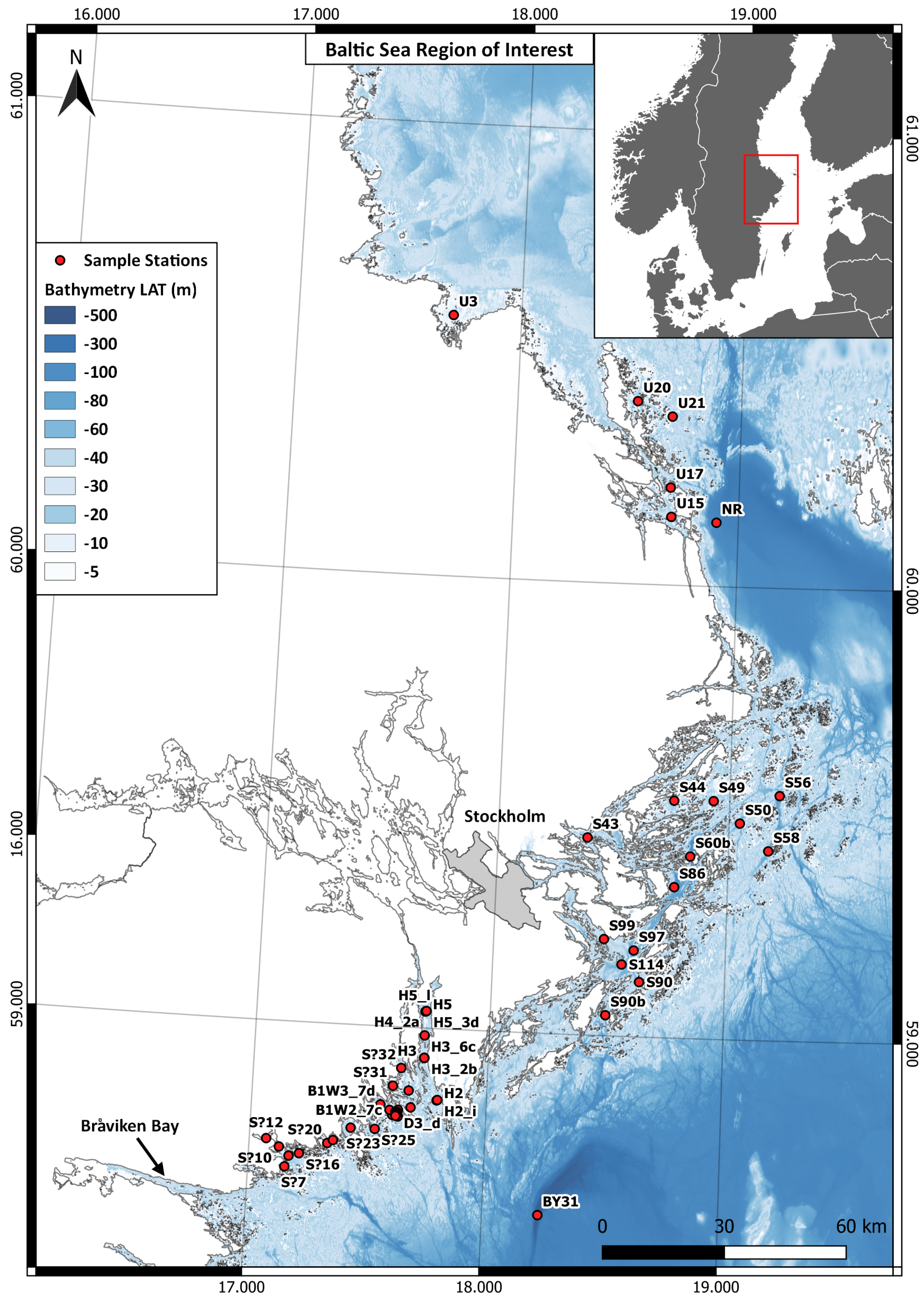
Figure 2.
C2RCC v2.1 validation workflow diagram for both the SVC and non-SVC regionally adapted C2RCC processing chains. The C2RCC v1.0 processing workflow was identical, apart from the processor version. The default, non-regionally adapted, C2RCC parameters were also validated. âKYKRâ refers to the in situ dataset from Kyryliuk and Kratzer [15], âPLKRâ refers to the Kratzer and Plowey [16] dataset, and âMGâ is the Swedish National Marine Monitoring Program (SwAM) dataset. âPix Extâ refers to âPixel Extractionâ.
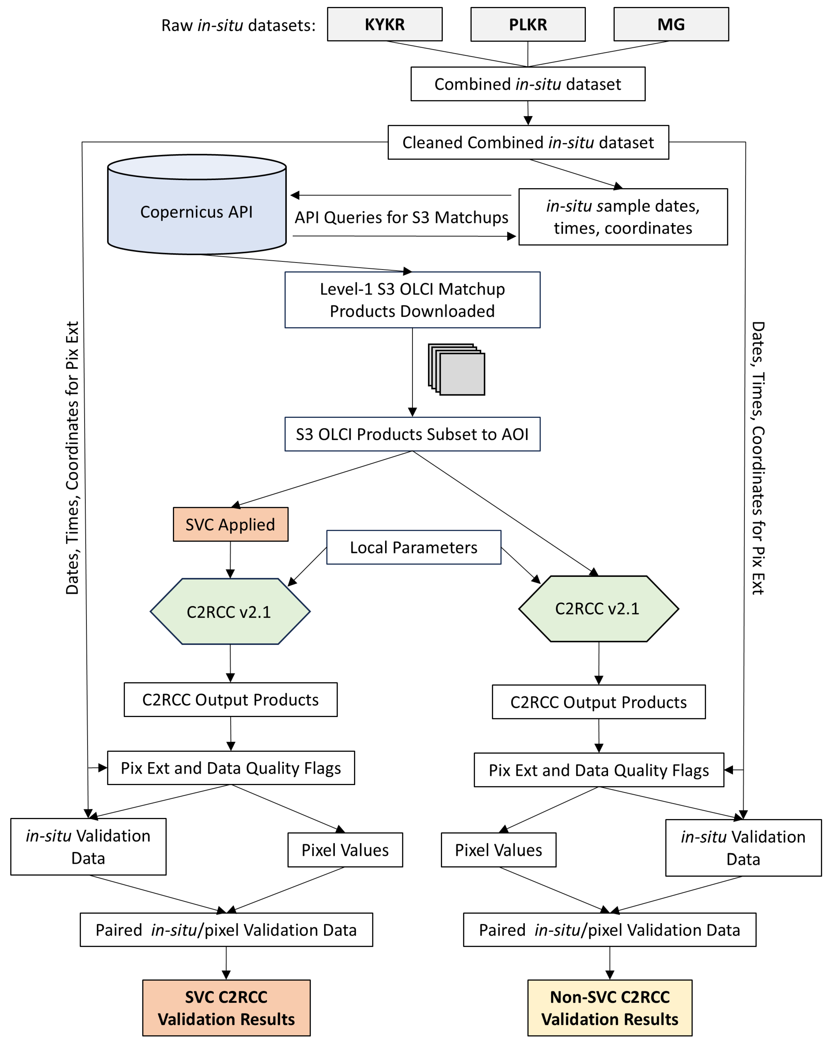
Figure 3.
EUMETSAT Level-2 Sentinel-3 OLCI-A and OLCI-B Level-2 standard products validation workflow diagram. âPix Extâ refers to âPixel Extractionâ.
Figure 3.
EUMETSAT Level-2 Sentinel-3 OLCI-A and OLCI-B Level-2 standard products validation workflow diagram. âPix Extâ refers to âPixel Extractionâ.
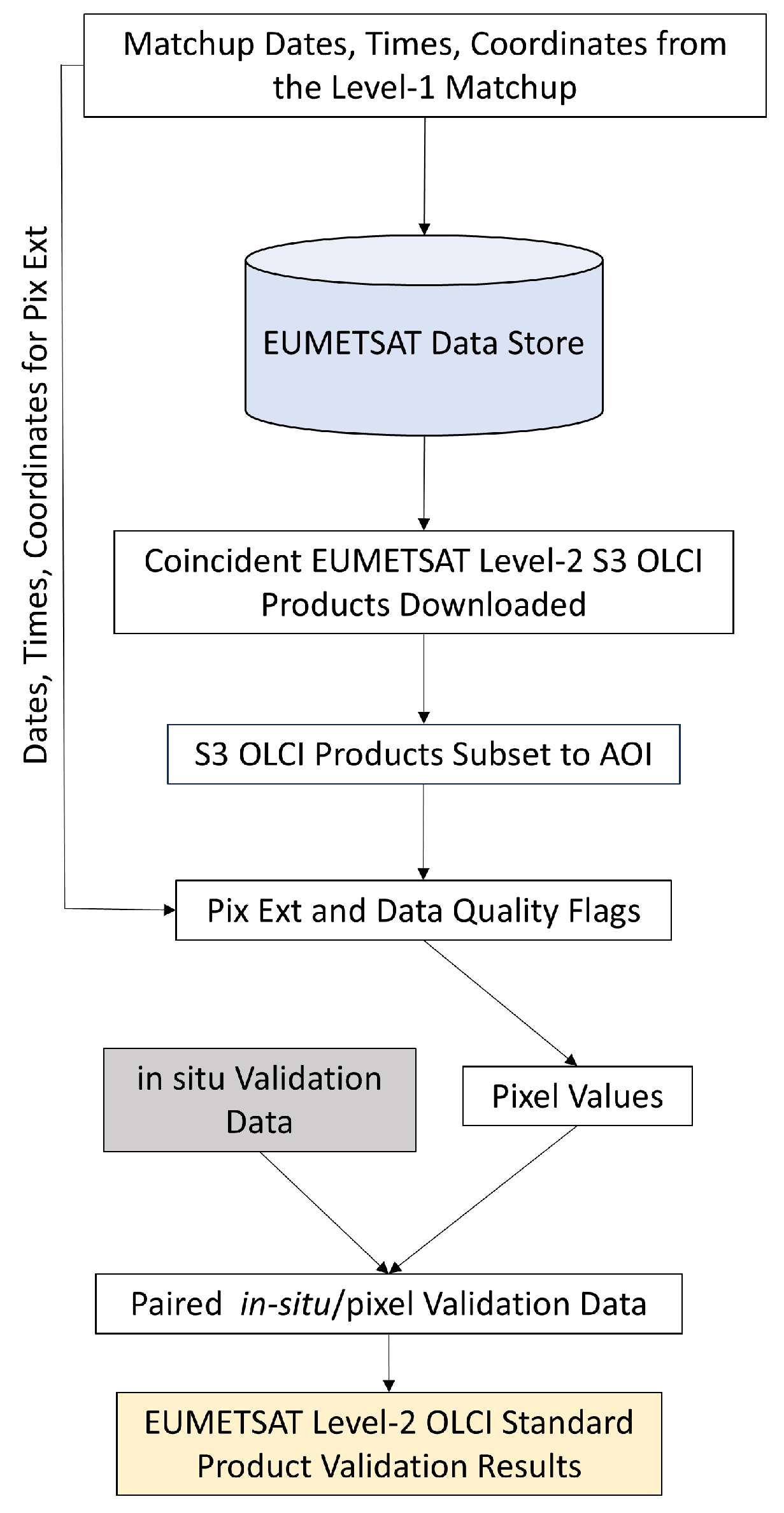
Figure 4.
SVC gains for OLCI-A, Collection OL_L2M.003. Adapted from [11].
Figure 4.
SVC gains for OLCI-A, Collection OL_L2M.003. Adapted from [11].

Figure 5.
SVC gains for OLCI-B in Collection OL_L2M.003. Adapted from [11].
Figure 5.
SVC gains for OLCI-B in Collection OL_L2M.003. Adapted from [11].
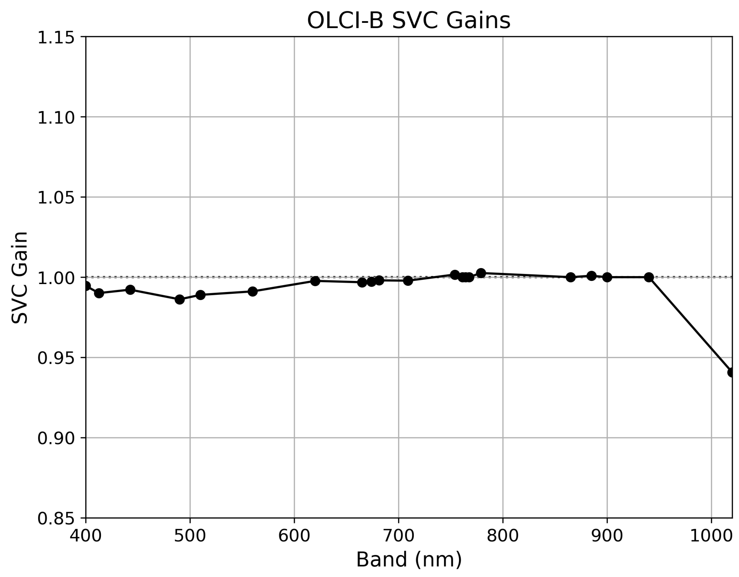
Table 2.
OLCI data quality flags evaluated from [15,16,40], alongside the final flags used for the C2RCC validation. Those highlighted in grey are the baseline quality flags used by [15].
| OLCI Quality Flags Tested | Final Quality Flags |
|---|---|
| && !quality_flags.land | c2rcc_flags.Valid_PE |
| && !quality_flags.bright | && !c2rcc_flags.Cloud_risk |
| && !quality_flags.straylight_risk | && !c2rcc_flags.Rhow_OOS |
| && !quality_flags.invalid | && !c2rcc_flags.Rtosa_OSS |
| && !quality_flags.cosmetic | && !quality_flags.sun_glint_risk |
| && !quality_flags.sun_glint_risk | |
| && !quality_flags.dubious | Â Â Â Â Â |
Table 3.
EUMETSAT Baseline Collection 003 Sentinel-3 OLCI Level-2 standard productâs recommended data quality flags ([11]).
Table 3.
EUMETSAT Baseline Collection 003 Sentinel-3 OLCI Level-2 standard productâs recommended data quality flags ([11]).
| EUMETSAT Standard Products Quality Flags |
|---|
| WQSF_lsb.WATER |
| AND NOT WQSF_lsb.INVALID |
| AND NOT WQSF_lsb.LAND |
| AND NOT WQSF_lsb.COSMETIC |
| AND NOT WQSF_lsb.SUSPECT |
| AND NOT WQSF_lsb.CLOUD |
| AND NOT WQSF_lsb.CLOUD_AMBIGUOUS |
| AND NOT WQSF_lsb.CLOUD_MARGIN |
| AND NOT WQSF_lsb.SNOW_ICE |
| AND NOT WQSF_lsb.HISOLZEN |
| AND NOT WQSF_lsb.SATURATED |
| AND NOT WQSF_lsb.HIGHGLINT |
| AND NOT WQSF_lsb.OCNN_FAIL |
Table 4.
C2RCC OLCI output products (adapted from [44]). Products in bold are those products validated in this study.
Table 4.
C2RCC OLCI output products (adapted from [44]). Products in bold are those products validated in this study.
| Output Level-2 C2RCC OLCI Products | ||
|---|---|---|
| Product | Description | Unit |
| Reflectances | ||
| Rtoa 400â1020 nm | Top-of-atmosphere reflectance | |
| Rrs 400â1020 nm | Atmospherically corrected angular dependent remote sensing reflectances | sr-1 |
| Rhow 400â1020 nm | Normalized water leaving reflectances | |
| Diffuse attenuation coefficient | ||
| kd489 | Irradiance attenuation coefficient at 489 nm | m-1 |
| kdmin | Mean irradiance attenuation coefficient at the three bands with minimum kd | m-1 |
| kd_z90max | Depth of the water column from which 90% of the water-leaving irradiance comes from (1/kdmin) | m |
| Inherent optical properties | ||
| iop_apig | Absorption coefficient of phytoplankton pigments at 443 nm | m-1 |
| iop_adet | Absorption coefficient of detritus at 443 nm | m-1 |
| iop_agelb | Absorption coefficient of Gelbstoff at 443 nm | m-1 |
| iop_bpart | Scattering coefficient of marine particles at 443 nm | m-1 |
| iop_bwit | Scattering coefficient of white particles at 443 nm | m-1 |
| iop_adg | Detritus + gelbstoff absorption at 443 nm (iop_adet + iop_agelb) | m-1 |
| iop_atot | Phytoplankton + detritus + gelbstoff absorption at 443 nm (iop_apig + iop_adet + iop_agelb) | m-1 |
| iop_btot | Total particle scattering at 443 nm (iop_bpart + iop_bwit) | m-1 |
| Concentrations | ||
| conc_tsm | Total suspended matter dry weight concentration (v1.0: TSM = iop_bpart à 0.986 + iop_bwit à 1.72; v2.1: TSM = TSMfac * iop_btotT̂SMexp ) | gm-3 |
| conc_chl | Chlorophyll concentration (pow (iop_apig, 1.04) Ã 21.0) | mg m-3 |
Table 5.
*5°C for April, May, October, 15°C for June, July, August, September; **New default value in C2RCC v2.1. The âv1.0 Reg Adapâ parameters are the same as those used by [15], except for the salinity parameter which was changed from a value of 7 PSU to a value of 6.5 PSU. âv1.0 Reg Adapâ: C2RCC v1.0 with regionally adapted TSM parameters; âv2.1 Reg Adapâ: C2RCC v2.1 with regionally adapted TSM parameters (same parameters used for âv2.1 Reg Adap SVCâ); âv2.1 Defâ: C2RCC v2.1 with default TSM parameters (same parameters used for âv2.1 Default SVCâ).
| C2RCC OLCI Processing Parameters | |||
|---|---|---|---|
| v1.0 Reg Adap | v2.1 Def | v2.1 Reg Adap | |
| Valid-pixel Expression | default | default | default |
| Salinity | 6.5 | 6.5 | 6.5 |
| Temperature | 5, 15 * | 5, 15 * | 5, 15 * |
| Ozone | 330 | 330 | 330 |
| Air Pressure | 1000 | 1000 | 1000 |
| TSM factor bpart (v1.0) | 0.986 | ||
| TSM factor bwit (v1.0) | 1.72 | ||
| TSM factor (v2.1) | 1.06 | 1.212 | |
| TSM exponent (v2.1) | 0.942 | 0.686 | |
| CHL exponent | 1.04 | 1.04 | 1.04 |
| CHL Factor | 21 | 21 | 21 |
| Threshold rtosa OOS | 0.05 | 0.01** | 0.01** |
| Threshold AC reflectances OOS | 0.1 | 0.15** | 0.15** |
| Threshold for cloud flag on transmittance down @865 | 0.955 | 0.955 | 0.955 |
| Atmospheric aux data path | default | default | default |
| Alternative NN path | default | default | default |
| Output AC reflectances as Rrs instead of rhow | On | On | On |
| Derive water reflectance from path radiance and transmittance | Off | Off | Off |
| Use ECMWF aux data of source product | On | On | On |
| Output TOA reflectance | On | On | On |
| Output gas corrected TOSA reflectance | Off | Off | Off |
| Output gas corrected TOSA reflectances of auto NN | Off | Off | Off |
| Output path radiance reflectance | Off | Off | Off |
| Output downward transmittance | Off | Off | Off |
| Output upward transmittance | Off | Off | Off |
| Output atmospherically corrected angular dependent reflectances | On | On | On |
| Output normalized water-leaving reflectance | On | On | On |
| Output of out of scope values | Off | Off | Off |
| Output of irradiance attenuation coefficients | On | On | On |
| Output uncertainties | On | On | On |
Table 6.
Validation results for C2RCC (v1.0 and v2.1) âconc_tsmâ for the Baltic Sea ROI, for both the ±2h and ±3h validation time windows. âReg Adapâ: regionally adapted TSM parameters. âDefaultâ: default C2RCC TSM parameters. âVal Rangeâ: validation data range. SVC results are highlighted in grey, while the best results are outlined in bold.
| v1.0 Reg Adap | v2.1 Default | v2.1 Default SVC | v2.1 Reg Adap | v2.1 Reg Adap SVC | |
|---|---|---|---|---|---|
| TSM / conc_tsm (±2h) | |||||
| Pearson R | 0.64 | 0.87 | 0.74 | 0.84 | 0.72 |
| MNB | 85% | 144% | 182% | 135% | 158% |
| RMSD | 152% | 202% | 251% | 179% | 209% |
| MAPD/APD | 105% | 151% | 186% | 140% | 161% |
| N = | 47 | 39 | 41 | 39 | 41 |
| Val Range (g m3) | 0.28 - 6.17 | 0.28 - 6.17 | 0.28 - 6.17 | 0.28 - 6.17 | 0.28 - 6.17 |
| TSM / conc_tsm (±3h) | |||||
| Pearson R | 0.65 | 0.87 | 0.68 | 0.85 | 0.66 |
| MNB | 92% | 146% | 188% | 133% | 162% |
| RMSD | 164% | 202% | 258% | 176% | 212% |
| MAPD/APD | 111% | 151% | 192% | 137% | 165% |
| N = | 66 | 59 | 59 | 59 | 59 |
| Val Range (g m3) | 0.28 - 6.17 | 0.28 - 6.57 | 0.28 - 6.17 | 0.28 - 6.57 | 0.28 - 6.17 |
Table 7.
C2RCC âv1.0â (no SVC), âv2.1â (no SVC), and âv2.1 SVCâ (including SVC) validation results for: âconc_chlâ, âiop_agelbâ, âiop_adgâ and âkd_z90maxâ. âVal Rangeâ: validation data range. SVC results are highlighted in grey, while the best validation results are outlined in bold.
Table 7.
C2RCC âv1.0â (no SVC), âv2.1â (no SVC), and âv2.1 SVCâ (including SVC) validation results for: âconc_chlâ, âiop_agelbâ, âiop_adgâ and âkd_z90maxâ. âVal Rangeâ: validation data range. SVC results are highlighted in grey, while the best validation results are outlined in bold.
| v1.0 (±2h) | v1.0 (±3h) | v2.1 (±2h) | v2.1 SVC (±2h) | v2.1 (±3h) | v2.1 SVC (±3h) | |
|---|---|---|---|---|---|---|
| Chl-a / conc_chl | ||||||
| Pearson R | 0.49 | 0.47 | 0.68 | 0.4 | 0.64 | 0.4 |
| MNB | -15% | -20% | 17% | 77% | 15% | 67% |
| RMSD | 67% | 66% | 57% | 194% | 56% | 174% |
| MAPD/APD | 56% | 56% | 45% | 95% | 43% | 84% |
| N | 128 | 171 | 120 | 125 | 161 | 164 |
| Val Range (μg L-1) | 1.09 - 28.58 | 1.07 - 28.58 | 1.09 - 28.58 | 1.02 - 28.58 | 1.07 - 28.58 | 1.02 - 28.58 |
| CDOM / iop_agelb | ||||||
| Pearson R | 0.53 | 0.57 | 0.57 | 0.23 | 0.16 | 0.24 |
| MNB | -69% | -70% | -80% | -57% | -74% | -65% |
| RMSD | 72% | 74% | 81% | 136% | 85% | 118% |
| MAPD/APD | 69% | 70% | 80% | 97% | 83% | 90% |
| N | 36 | 55 | 29 | 30 | 48 | 48 |
| Val Range (m-1) | 0.33 - 1.4 | 0.28 - 1.4 | 0.33 - 1.4 | 0.33 - 1.4 | 0.28 - 1.4 | 0.28 - 1.4 |
| CDOM / iop_adg | ||||||
| Pearson R | 0.7 | 0.72 | 0.74 | 0.42 | 0.55 | 0.44 |
| MNB | -26% | -32% | -39% | -1% | -35% | -13% |
| RMSD | 60% | 61% | 51% | 138% | 62% | 112% |
| MAPD/APD | 55% | 55% | 47% | 61% | 51% | 51% |
| N | 36 | 55 | 29 | 30 | 48 | 48 |
| Val Range (m-1) | 0.33 - 1.4 | 0.28 - 1.4 | 0.33 - 1.4 | 0.33 - 1.4 | 0.28 - 1.4 | 0.28 - 1.4 |
| Secchi depth / kd_z90max | ||||||
| Pearson R | 0.12 | 0.14 | 0.59 | 0.15 | 0.5 | 0.13 |
| MNB | 26% | 26% | -34% | -48% | -33% | -45% |
| RMSD | 124% | 120% | 41% | 54% | 42% | 52% |
| MAPD/APD | 65% | 63% | 37% | 50% | 38% | 48% |
| N | 39 | 53 | 40 | 38 | 53 | 52 |
| Val Range (m) | 3.0 - 10.6 | 3.0 - 11.0 | 3.0 - 10.6 | 3.0 - 10.6 | 3.0 - 11.0 | 3.0 - 11.0 |
Table 8.
EUMETSAT Sentinel-3 OLCI-A and OLCI-B Level-2 NN standard products validation results. Both ±2h and ±3h matchup time windows were validated. âVal Rangeâ: validation data range. The best validation results are highlighted in bold.
Table 8.
EUMETSAT Sentinel-3 OLCI-A and OLCI-B Level-2 NN standard products validation results. Both ±2h and ±3h matchup time windows were validated. âVal Rangeâ: validation data range. The best validation results are highlighted in bold.
| TSM / TSM_NN | ||
|---|---|---|
| TSM_NN (±2h) | TSM_NN (±3h) | |
| Pearson R | 0.77 | 0.66 |
| MNB | 209% | 201% |
| RMSD | 265% | 263% |
| MAPD/APD | 211% | 204% |
| N | 37 | 56 |
| Val Range (g m3) | 0.28 - 4.49 | 0.28 - 4.49 |
| Chl-a / CHL_NN | ||
| CHL_NN (±2h) | CHL_NN (±3h) | |
| Pearson R | 0.48 | 0.43 |
| MNB | 75% | 63% |
| RMSD | 135% | 121% |
| MAPD/APD | 89% | 78% |
| N | 127 | 173 |
| Val Range (μg L-1) | 1.09 - 28.58 | 1.07 - 28.58 |
| CDOM / ADG443_NN | ||
| ADG443_NN (±2h) | ADG443_NN (±3h) | |
| Pearson R | 0.36 | 0.39 |
| MNB | -12% | -14% |
| RMSD | 66% | 69% |
| MAPD/APD | 44% | 46% |
| N | 29 | 47 |
| Val Range (m-1) | 0.3 - 0.7 | 0.29 - 0.7 |
Disclaimer/Publisher’s Note: The statements, opinions and data contained in all publications are solely those of the individual author(s) and contributor(s) and not of MDPI and/or the editor(s). MDPI and/or the editor(s) disclaim responsibility for any injury to people or property resulting from any ideas, methods, instructions or products referred to in the content. |
© 2024 by the authors. Licensee MDPI, Basel, Switzerland. This article is an open access article distributed under the terms and conditions of the Creative Commons Attribution (CC BY) license (http://creativecommons.org/licenses/by/4.0/).
Copyright: This open access article is published under a Creative Commons CC BY 4.0 license, which permit the free download, distribution, and reuse, provided that the author and preprint are cited in any reuse.


