

Submitted:
30 July 2024
Posted:
31 July 2024
You are already at the latest version
Abstract
Neural Fractional Differential Equations (Neural FDE) represent a neural network architecture specifically designed to fit the solution of a fractional differential equation to given data. This architecture combines an analytical component, represented by a fractional derivative, with a neural network component, forming an initial value problem. During the learning process, both the order of the derivative and the parameters of the neural network must be optimised. In this work, we investigate the non-uniqueness of the optimal order of the derivative and its interaction with the neural network component. Based on our findings, we perform a numerical analysis to examine how different initialisations and values of the order of the derivative (in the optimisation process) impact its final optimal value. Results show that the neural network on the right-hand side of the Neural FDE struggles to adjust its parameters to fit the FDE to the data dynamics for any given order of the fractional derivative. Consequently, Neural FDEs do not require a unique α value, instead, they can use a wide range of α values to fit data. This flexibility is beneficial when fitting to given data is required, and the underlying physics is not known.
Keywords:
Fractional Differential Equations
; Neural Networks
; Optimisation
1. Introduction
Real-world systems are often modelled using integral/differential equations, which are then numerically solved to predict the system behaviour and evolution. This process can be time-consuming, as numerical simulations sometimes take months, and, finding the correct model parameters is often challenging. However, with significant advancements in Neural Networks (NNs) that can learn patterns, real-world systems are increasingly being modelled using a combination of integral/differential models and NNs, or even NNs alone [1,2,3,4].
Neural Ordinary Differential Equations (Neural ODEs) were introduced in 2018 [5] (see also [6,7]) as a continuous version of the discrete Residual Neural Networks, and claimed to offer a continuous modelling solution for real-world systems that incorporate time-dependence, mimicking the dynamics of that system using only discrete data. Once trained, the Neural ODEs result in a hybrid ODE (part analytical, part NN-based) that can be used for making predictions, by numerically solving the resulting ODEs. The numerical solution of these hybrid ODEs is significantly simpler and less time-consuming compared to the numerical solution of complex governing equations, making Neural ODEs an excellent choice for modelling time-dependent real-world systems. However, the simplicity of ODEs sometimes limits their effectiveness in capturing complex behaviours characterised by intricate dynamics, non-linear interactions, and memory. To address this, Neural Fractional Differential Equations (Neural FDEs) were recently proposed [8,9].
Neural FDEs, as described by Equation (1), are a NN architecture designed to fit the solution to given data (for example, experimental data), over a specified time range . The Neural FDE combines an analytical part, , with a NN-based part, , leading to the initial value problem,
Here, denotes the Caputo fractional derivative [10,11], defined for (and considering a generic scalar function ) as:
where is the Gamma function.
An important feature of Neural FDEs is their ability to learn not only the optimal parameters of the NN , but also the order of the derivative (when we obtain a Neural ODE). This is achieved using only information from the time-series dataset , where each , is associated with a time instant .
In [9] the value is learned from another NN with parameters . Therefore, if represents the loss function, we can train the Neural FDE by solving the minimisation problem (Section 1). The parameters and are optimised by minimising the error between the predicted and ground-truth values1:
 The popular Mean Squared Error (MSE) loss function was considered in [9] and also in this work. Here, refers to any numerical solver used to obtain the numerical solution for each instant .
Since Neural FDEs are a recent research topic, there are no studies on the uniqueness of the parameter and its interaction with the NN . In [9], the authors provide the values of learned by Neural FDEs for each dataset, however, a closer examination reveals that these values differ significantly from the ground truth values, which were derived from synthetic datasets. The authors attribute this discrepancy to the approximation capabilities of NNs, meaning that, during training, adapts to any given (this is a complex interaction since in [9], is also learned by another NN). Additionally, must be initialised in the optimisation procedure, and yet no studies have investigated how the initialisation of affects the learned optimal and the overall performance of Neural FDEs.
In this work, we address these key open questions about the order of the fractional derivative in Neural FDEs. We show that Neural FDEs are capable of modelling data dynamics effectively, even when the learned value of deviates significantly from the true value. Furthermore, we perform a numerical analysis to investigate how the initialisation of affects the performance of Neural FDEs.
This paper is organised as follows: In Section 2, we provide a brief overview of FDEs and Neural FDEs, highlighting the theoretical results regarding the existence and uniqueness of solutions. We also discuss how the solution depends on the given data. Section 3 presents a series of numerical experiments on the non-uniqueness of the learnt values. The paper ends with the discussion and conclusions in Section 4.
2. Neural Networks and Theory of Fractional Initial Value Problems
As shown in the introduction, a Neural FDE is composed of two NN:
- a NN with parameters , denoted as , that models the right-hand side of a FDE,where is the state of the system at time-step t;
- a NN with parameters (or a learnable parameter), referred to as , that models ,
As shown in Figure 1 in this work we constructed with 3 layers: input layer with 1 neuron and hyperbolic tangent (tanh) activation function; hidden layer with 64 neurons and tanh; output layer with 1 neuron. For learning we considered a NN with 3 layers: input layer with 1 neuron and hyperbolic tangent (tanh) activation function; hidden layer with 32 neurons and tanh; output layer with 1 neuron and sigmoid activation function (that helps keeping the value of in the interval ). For ease of understanding we consider to be a scalar in Figure 2 and in Equations (6) and (7). We use instead of , because it is assumed that is being evaluated during the training of the Neural FDE, where a numerical solution is needed ( is a numericall approximation of [9]). After training, we obtain the final/optimal Neural FDE model and use again the notation .
In the NN (Figure 1), the values and for are the weights of the hidden and output layers, respectively, and b is the bias, . The output of the NN can be written as,
An important feature is that there is no activation function in the output layer of , allowing the NN to approximate any function . If we opt to use, for example, a tanh in the output layer, it would constrain the fractional derivative to vary only from -1 to 1, thus limiting the fitting capabilities of the Neural FDE. This limitation could be mitigated by normalising the given data .
Remark: In Figure 1 and Equation (6), we observe h as a function of t. However, the NN depicted on the left side of Figure 1 does not use t as an input. Instead, the NN is called at each iteration of the numerical solver that addresses a discretised version of Equation (1). This solver defines all time instants through a mesh over the interval [9], and, consequently, each evaluation of is always associated with a specific time instant.
Since for a differentiable function with continuous derivative on we have that (using the mean value Theorem),
and (), we can say that tanh is 1-Lipschitz, that is,
Define as,
which is a weighted sum of 64 tanh functions. Then, is L-Lipschitz, with (). This property will be important to guarantee the uniqueness of the solution of (1).
2.1. Fractional Differential Equations
We now provide some theoretical results that will be fundamental in understanding the expected behaviour of the Neural FDE model. Consider the following fractional initial value problem,
For ease of understanding we restrict the analyses to the case where is a scalar function and .
2.1.1. Existence and Uniqueness
The following Theorem [11,12] provides information on the existence of a continuous solution to problem (8):
Theorem 1.
Let , , and . Define , and let the function be continuous. Furthermore, we define and
Then, there exists a function solving the initial value problem (8).
Note that this continuous solution may be defined in a smaller interval compared to the interval where the function is defined (). From Theorem (1), we can infer that high values of (see Equation (1)) decrease the interval within which we can guarantee a continuous solution. However, these conclusions should be approached with caution. As will be shown later, we will only access discrete values of the function in the numerical solution of (1). Note that also affects the size of the interval. Its contribution can be either positive or negative, depending on the values of Q and M.
The following Theorem establishes the conditions for which we can guarantee the uniqueness of the solution [11,12]:
Theorem 2.
Let , , and . Define the set and let the function be continuous and satisfy a Lipschitz condition with respect to the second variable:
where is a constant independent of t, , and . Then, there exists a uniquely defined function solving the initial value problem (8).
2.1.2. Analysing the Behaviour of Solutions with Perturbed Data
Other results of interest for Neural FDEs pertain to the dependencies of the solution on and . In Neural FDEs, both and are substituted by NNs that vary with each iteration of the Neural FDE training [9].
Let be the solution of the initial value problem,
where is a perturbed version of f, that satisfies the same hypotheses as
Theorem 3.
This Theorem provides insight into how the solution of (1) changes in response to variations in the NN . While the variations in both the solution and the function are of the same order for small changes of the function, it is crucial to carefully interpret these results given the NN as defined by Equation (7).
When training the Neural ODE, one must solve the optimisation problem (Section 1), where the weights and biases are adjusted until an optimal Neural FDE model is obtained (training 1). If a second, independent training (training 2) of the Neural FDE is conducted with the same stopping criterion for the optimisation process, a new Neural FDE model with different weights and biases may be obtained.
The NN learns model parameters based on a set of ordered data, meaning the number of elements in the set will significantly influence the difference between and as in Theorem (3). This effect is illustrated in Figure 2, where a training dataset of only two observations can be fitted by two distinct functions.
Therefore, Figure 2 tells us that when modelling with Neural FDEs, it is important to have some prior knowledge of the underlying physics of the data. This is crucial because the number of data points available for the training process might be beyond our control. For instance, the data could originate from real experiments where obtaining results is challenging.
Theorem 4.
Let be the solution of the initial value problem,
where is a perturbed α value. Let . Then, if ε is sufficiently small, there exists some such that both the functions u and z are defined on , and we have that
where is the solution of (8).
Once again, for small changes in , the variations in both the solution and the order of the derivative are of the same order. This property will be explored numerically, and with more detail, later in this work when solving (Section 1). It is important to note that the NN is not fixed in our problem (1) (its structure is fixed, but the weights and bias change along the training optimisation procedure). However, Theorem (4) assumes that the function is fixed. Therefore, Theorem (4) gives us an idea of the changes in our solution, but does not allow the full understanding of its variation along the optimisation procedure.
2.1.3. Smoothness of the Solution
For the classical case, in Equation (8), we have (under some hypotheses on the interval ) that if , then is k times differentiable.
For the fractional case, even if , it may happen that . This means that the solutions may not behave well, and solutions with singular derivatives are quite common. See [13] for more results on the smoothness properties of solutions to fractional initial value problems.
These smoothness properties (or lack of smoothness) make it difficult for numerical methods to provide fast and accurate solutions for (1), thus making Neural FDEs more difficult to handle compared to Neural ODEs. It should be highlighted that during the learning process, the NN will always adjust the Neural FDE model to the data, independent of the amount of error obtained in the numerical solution of the FDE.
3. Neural Fractional Differential Equations and the Learned Order of the Derivative -
In Neural FDEs, the goal is to model systems where the order of the derivative, , is a parameter that needs to be learned along with the parameters of a NN . A key challenge in this approach is the potential variability and non-uniqueness of the learned values, especially when the ground-truth used to generate synthetic datasets is known a priori. This variability arises from the highly flexible nature of NNs, which can adjust their parameters to fit the data well, regardless of the specific value of .
3.1. Numerical Experiments
The results obtained in [9] propose the existence of parameters and corresponding parameter vectors , that satisfy the following condition:
In theory, this implies that for each i, the loss function can converge to zero.
There are some results in the literature on the universal approximation capabilities of Neural ODEs and ResNets. Interested readers should consult [14,15] for more information.
Based on these observations, we now conduct numerical experiments to observe in detail the practical outcomes. Specifically, we employ a Neural FDE to model population dynamics with different ground-truth values. Our goal is to examine how different initialisations of impact the final learned values.
We analyse the values learned across multiple runs and observe how evolves during training. Additionally, we fix the value and allow the Neural FDE to learn only the right-hand side of the FDE, comparing the loss for different values.
Consider a population of organisms that follows a fractional-order logistic growth. The population size at time t is governed by the following FDE of order :
with initial condition , a growth-rate and carrying capacity .
To conduct the experiments, three training datasets were generated by numerically solving (12) over the interval with a step size of for three different values of , namely . These datasets are denoted as , , and , respectively. For the experiments, Adam optimiser [16] was used with a starting learning rate of 1E-03.
3.1.1. Case Study 1: varying and fixed number of iterations
The generated datasets were used to train the Neural FDE model (see Equation (1)) with four different initialisations of the derivative order: , , , and . For each initialisation, three independent runs were conducted considering 200 iterations.
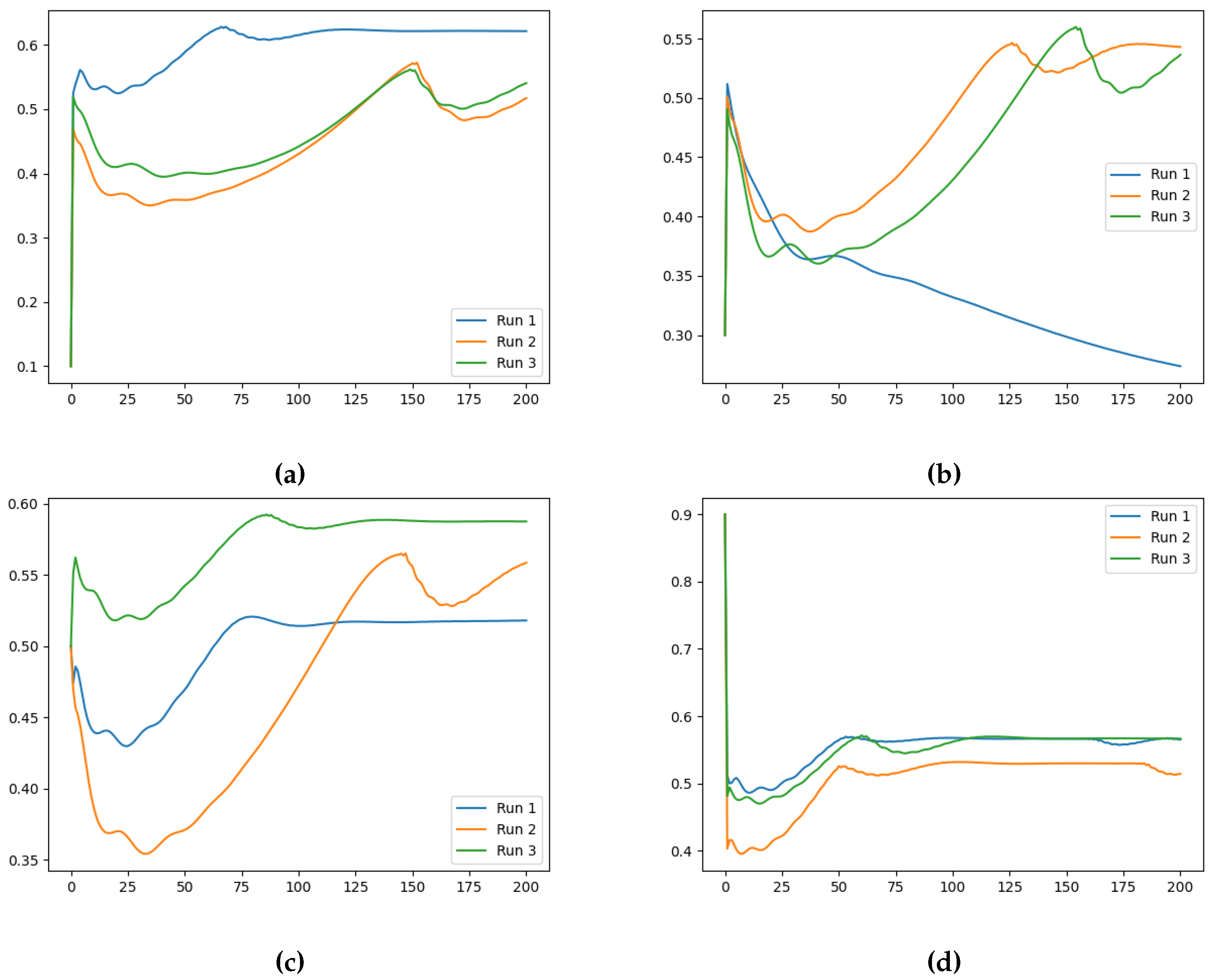
The results obtained for each dataset, , , and , using the various initialisation values are presented in Table 1, Table 2 and Table 3 and the evolution of the training losses and values can be visually observed in Figure 3, Figure A1-Figure A2 and Figure 4, Figure A3, Figure A4, respectively.
The results presented in Table 1 through Table 3 indicate that the initial value of does not significantly impact the final learned value of . While there is some effect, it is challenging to discern a clear pattern, and the observed variations fall within a certain range of randomness. However, the ground-truth value of in the datasets influences the learnt value, with higher ground-truth values leading to higher learnt values. For example, in Table 3, all learnt values are above , whereas for other datasets, the learnt values are lower. This is expected since the Neural FDE model should fit the given data (that depends on ).
Furthermore, the results demonstrate the approximation capabilities of NNs, which allow them to model the data dynamics with low errors even when the learnt is far from the ground-truth value. For example, in Table 1, the ground-truth is , but the lowest training loss was achieved with a learnt of . Similarly, in Table 3, the ground-truth is , but the lowest training loss values were achieved with learnt of and . It is interesting to note that the values of are significantly different from 1. The results obtained suggest that the optimisation procedure may be placing greater importance on the NN .
The evolution of the loss and the learned values along training (Figure 3 and Figure 4, respectively, for the case ), indicate that the initialisation and the ground-truth do not significantly influence the Neural FDE training process. In Figure 4 a pattern is observed. Initially the values increase drastically, and then slowly decrease approaching a plateau. In some cases, after around 100 iterations, the values begin to increase again. This behaviour results from the complex interplay between the two different NNs. The behaviour is even more irregular for the cases , as shown in Appendix A.
3.1.2. Case Study 2: fixed and fixed number of iterations
To demonstrate the effectiveness of Neural FDEs in minimising the loss function for various values, we performed experiments with fixed values of , , and . In these experiments, the Neural FDEs used exclusively the NN , to fit the solution to the three distinct datasets . The experimental conditions remained the same, except that was not learnable. Note that the stopping criterion was set to a fixed number of iterations, specifically 200.
The final training losses obtained for three runs, for each fixed , are summarised in Table 4, Table 5 and Table 6. The evolution of the training losses can be visualised in Figure 5, Figure 6 and Figure 7.
3.1.3. Case Study 3: fixed and fixed loss threshold
As a final experiment, we aimed to numerically demonstrate that Neural FDEs are capable of achieving the same fit to the data independent of the order. To unequivocally show this, we modified the stopping criteria of our Neural FDE training from a maximum number of iterations to a loss threshold of 1E-05. This approach ensures that the Neural FDEs are trained until the threshold is achieved, allowing us to demonstrate that they can reach the same loss values regardless of the value.
In this experiment, we performed one run for each dataset , , and with fixed values of 0.1, 0.3, 0.5, and 0.99. The results are organised in Table 7, Table 8 and Table 9
The results presented in Table 7 through Table 9 show that the NN is capable of optimising the parameters to accurately model the Neural FDE to the data dynamics, regardless of whether the imposed value of is close to or far from the ground truth.
These results might lead some to believe that changing does not impact memory. They might also suggest that the Neural FDE can model systems with varying memory levels, independent of . Although, this only happens because the NN , which models the FDE’s right-hand side, adjusts its parameters to fit the FDE for any value (effectively mimicking the memory effects associated with ). Therefore, Neural FDEs do not need a unique value for each dataset. Instead, they can work with an infinite number of values to fit the data. This flexibility is beneficial when fitting to given data is required, and the underlying physics is not known.
4. Conclusions
In this work, we present the theory of fractional initial value problems and explore its connection with Neural Fractional Differential Equations (Neural FDEs). We analyse both theoretically and numerically how the solution of a Neural FDE is influenced by two factors: the NN , which models the right-hand side of the FDE, and the NN that learns the order of the derivative.
We also investigate the numerical evolution of the order of the derivative () and training loss across several iterations, considering different initialisations of the value. For this experiment, with a fixed number of 200 iterations, we create three synthetic datasets for a fractional initial value problem with ground-truth values of 0.3, 0.5, and 0.99. We test four different initialisations for : 0.1, 0.3, 0.5, and 0.99. The results indicate that both the initial value and the ground-truth have minimal impact on the Neural FDE training process. Initially, the values increase sharply and then slowly decrease towards a plateau. In some cases, around 100 iterations, the values begin to rise again. This behaviour results from the complex interaction between the two NNs, and it is particularly irregular for and . The loss values achieved are low across all cases.
We then repeated the experiments, fixing the value, meaning there was no initialisation of , and the only parameters changing in the minimisation problem were those of the NN . The results confirm that the final training loss values are generally similar across different fixed values of . Even when the fixed matches the ground-truth of the dataset, the final loss remains comparable to other fixed values.
In a final experiment, we modified the stopping criteria of our Neural FDE training from a maximum number of iterations to a loss threshold. This ensures that the Neural FDEs are trained until the loss threshold is achieved, demonstrating that they can reach similar loss values regardless of the value. We conclude that, struggles to adjust its parameters to fit the FDE to the data for any given derivative order. Consequently, Neural FDEs do not require a unique value for each dataset. Instead, they can use a wide range of values to fit the data, suggesting that is a universal approximator.
If we train the model using data points obtained from an unknown experiment, then the flexibility of the Neural FDE proves to be an effective method for obtaining intermediate information about the system, provided the dataset contains sufficient information. If the physics involved in the given data is known, it is recommended to incorporate this knowledge into the loss function. This additional information helps to improve the extrapolation of results.
Funding
This work was also financially supported by national funds through the FCT/MCTES (PIDDAC), under the project 2022.06672.PTDC - iMAD - Improving the Modelling of Anomalous Diffusion and Viscoelasticity: solutions to industrial problems.
Acknowledgments
The authors acknowledge the funding by Fundação para a Ciência e Tecnologia (Portuguese Foundation for Science and Technology) through CMAT projects UIDB/00013/2020 and UIDP/00013/2020 and the funding by FCT and Google Cloud partnership through projects CPCA-IAC/AV/589164/2023 and CPCA-IAC/AF/589140/2023. C. Coelho would like to thank FCT the funding through the scholarship with reference 2021.05201.BD.
Appendix A. Evolution of loss and α along training
Figure A1.
Training loss evolution for Neural FDE when modelling for (a) , (b) , (c) and (d) initialisation (Loss (vertical axis) vs Number of Iterations (horizontal axis)).
Figure A1.
Training loss evolution for Neural FDE when modelling for (a) , (b) , (c) and (d) initialisation (Loss (vertical axis) vs Number of Iterations (horizontal axis)).
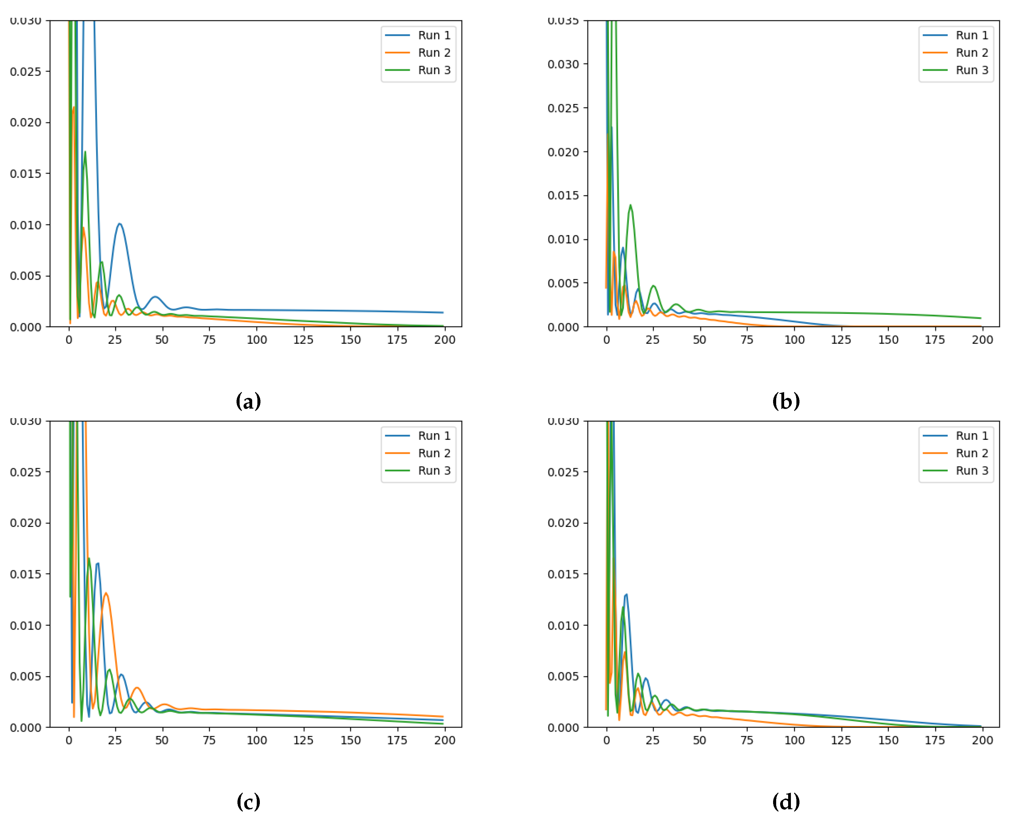
Figure A2.
Training loss evolution for Neural FDE when modelling for (a) , (b) , (c) and (d) initialisation (Loss (vertical axis) vs Number of Iterations (horizontal axis)).
Figure A2.
Training loss evolution for Neural FDE when modelling for (a) , (b) , (c) and (d) initialisation (Loss (vertical axis) vs Number of Iterations (horizontal axis)).
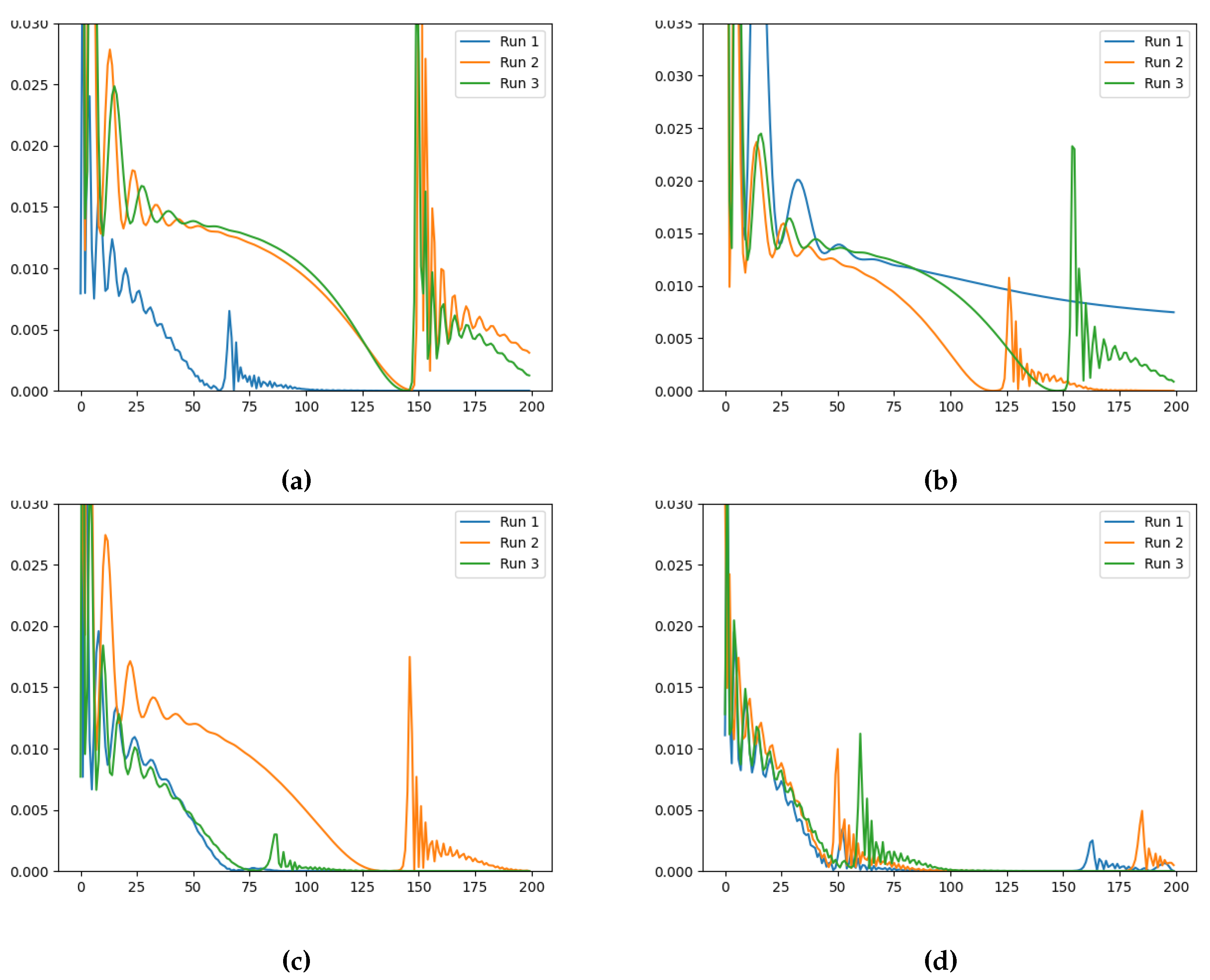
Figure A3.
Evolution of along the iterations. Case for (a) , (b) , (c) and (d) initialisation ( (vertical axis) vs Number of Iterations (horizontal axis)).
Figure A3.
Evolution of along the iterations. Case for (a) , (b) , (c) and (d) initialisation ( (vertical axis) vs Number of Iterations (horizontal axis)).
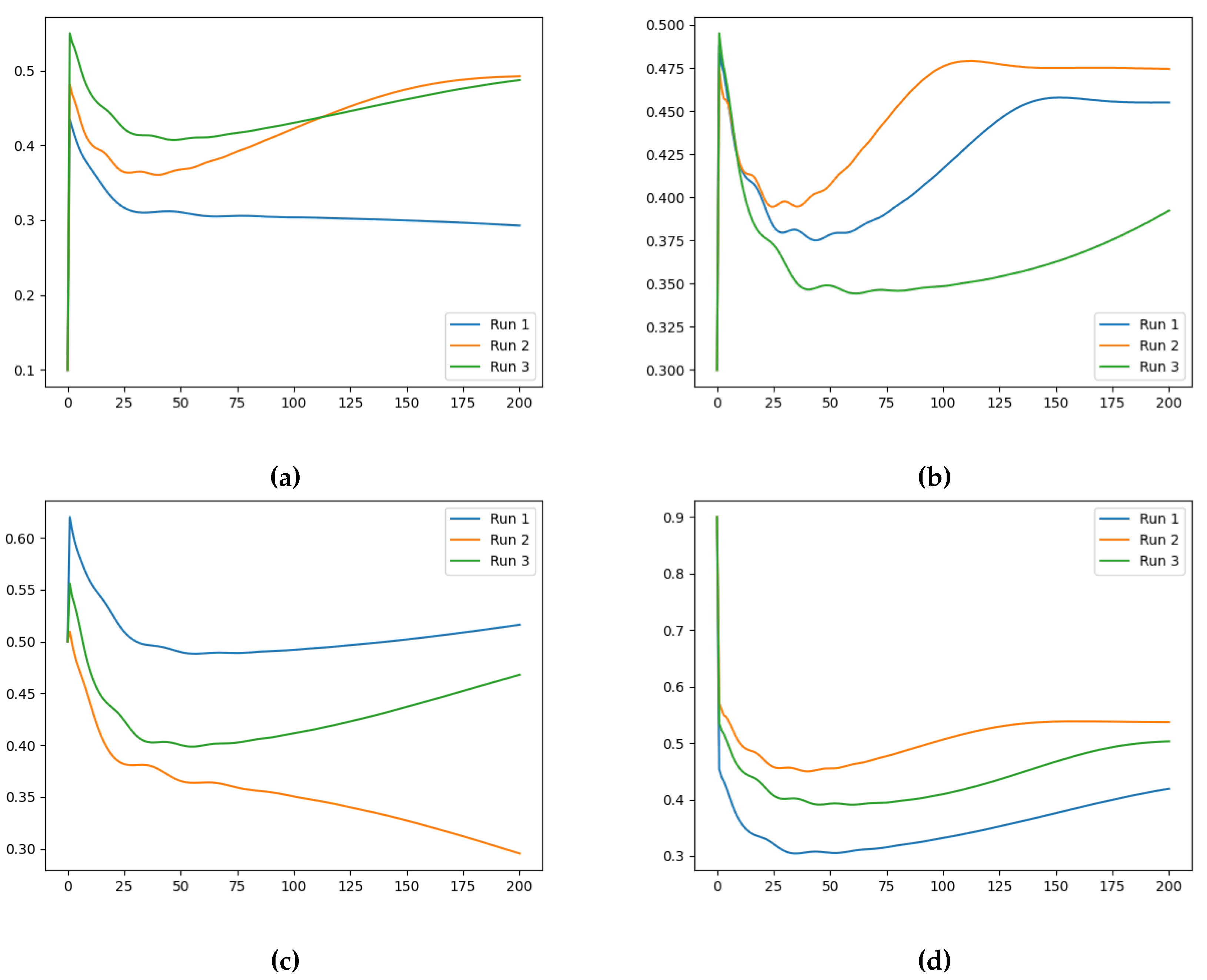
Figure A4.
Evolution of along the iterations. Case for (a) , (b) , (c) and (d) initialisation ( (vertical axis) vs Number of Iterations (horizontal axis)).
Figure A4.
Evolution of along the iterations. Case for (a) , (b) , (c) and (d) initialisation ( (vertical axis) vs Number of Iterations (horizontal axis)).
References
- Raissi, M.; Perdikaris, P.; Karniadakis, G. Physics-informed neural networks: A deep learning framework for solving forward and inverse problems involving nonlinear partial differential equations. Journal of Computational Physics 2019, 378, 686–707. [Google Scholar] [CrossRef]
- Salami, E.; Salari, M.; Ehteshami, M.; Bidokhti, N.; Ghadimi, H. Application of artificial neural networks and mathematical modeling for the prediction of water quality variables (case study: southwest of Iran). Desalination and Water Treatment 2016, 57, 27073–27084. [Google Scholar] [CrossRef]
- Jin, C.; Li, Y. Cryptocurrency Price Prediction Using Frequency Decomposition and Deep Learning. Fractal and Fractional 2023, 7, 708. [Google Scholar] [CrossRef]
- Ramadevi, B.; Kasi, V.R.; Bingi, K. Hybrid LSTM-Based Fractional-Order Neural Network for Jeju Island’s Wind Farm Power Forecasting. Fractal and Fractional 2024, 8, 149. [Google Scholar] [CrossRef]
- Chen, R.T.; Rubanova, Y.; Bettencourt, J.; Duvenaud, D.K. Neural ordinary differential equations. Advances in neural information processing systems 2018, 31. [Google Scholar]
- Massaroli, S.; Poli, M.; Park, J.; Yamashita, A.; Asama, H. Dissecting neural odes. Advances in Neural Information Processing Systems 2020, 33, 3952–3963. [Google Scholar]
- Dupont, E.; Doucet, A.; Teh, Y.W. Augmented neural odes. Advances in neural information processing systems 2019, 32. [Google Scholar]
- Coelho, C.; Costa, M.F.P.; Ferrás, L.L. Tracing footprints: Neural networks meet non-integer order differential equations for modelling systems with memory. The Second Tiny Papers Track at ICLR 2024, 2024. [Google Scholar]
- Coelho, C.; Costa, M.F.P.; Ferrás, L. Neural Fractional Differential Equations. arXiv 2024, arXiv:2403.02737. [Google Scholar]
- Caputo, M. Linear Models of Dissipation whose Q is almost Frequency Independent–II. Geophysical Journal International 1967, 13, 529–539. [Google Scholar] [CrossRef]
- Diethelm, K. , The Analysis of Fractional Differential Equations: An Application-Oriented Exposition Using Differential Operators of Caputo Type; Springer Berlin Heidelberg: Berlin, Heidelberg, 2010. [Google Scholar] [CrossRef]
- Diethelm, K.; Ford, N.J. Analysis of fractional differential equations. Journal of Mathematical Analysis and Applications 2002, 265, 229–248. [Google Scholar] [CrossRef]
- Diethelm, K. Smoothness properties of solutions of Caputo-type fractional differential equations. Fractional Calculus and Applied Analysis 2007, 10, 151–160. [Google Scholar]
- Zhang, H.; Gao, X.; Unterman, J.; Arodz, T. Approximation Capabilities of Neural ODEs and Invertible Residual Networks. Proceedings of the 37th International Conference on Machine Learning; III, H.D.; Singh, A., Eds. PMLR, 2020, Vol. 119, Proceedings of Machine Learning Research, pp. 11086–11095.
- Augustine, M.T. A Survey on Universal Approximation Theorems. arXiv 2024, arXiv:2407.12895. [Google Scholar]
- Kingma, D.P.; Ba, J. Adam: A method for stochastic optimization. arXiv 2014, arXiv:1412.6980. [Google Scholar]
| 1 | In this work we consider that the solution outputted by the solver is the predicted output, although this might not always be the case (e.g. image classification). |
Figure 1.
Schematic of the NNs ( and ) used in the Neural FDE. (Left) : The input refers to a single value while the output refers to a NN that will approximate a continuous function . and are the weights associated with the different layers. (Right) : the value of is initialised.
Figure 1.
Schematic of the NNs ( and ) used in the Neural FDE. (Left) : The input refers to a single value while the output refers to a NN that will approximate a continuous function . and are the weights associated with the different layers. (Right) : the value of is initialised.
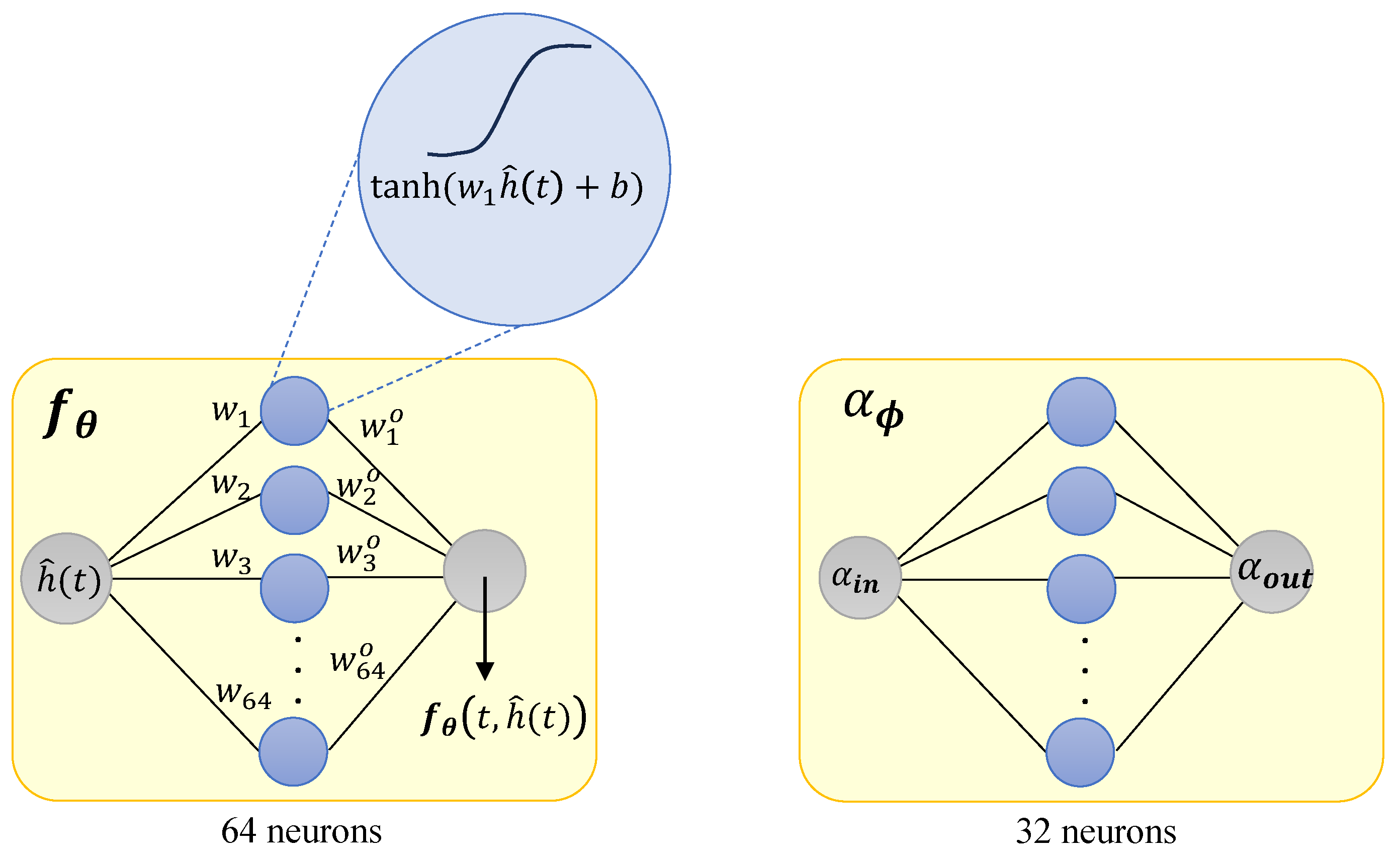
Figure 2.
Schematic of a Neural FDE model fitted to data, considering two different training runs.
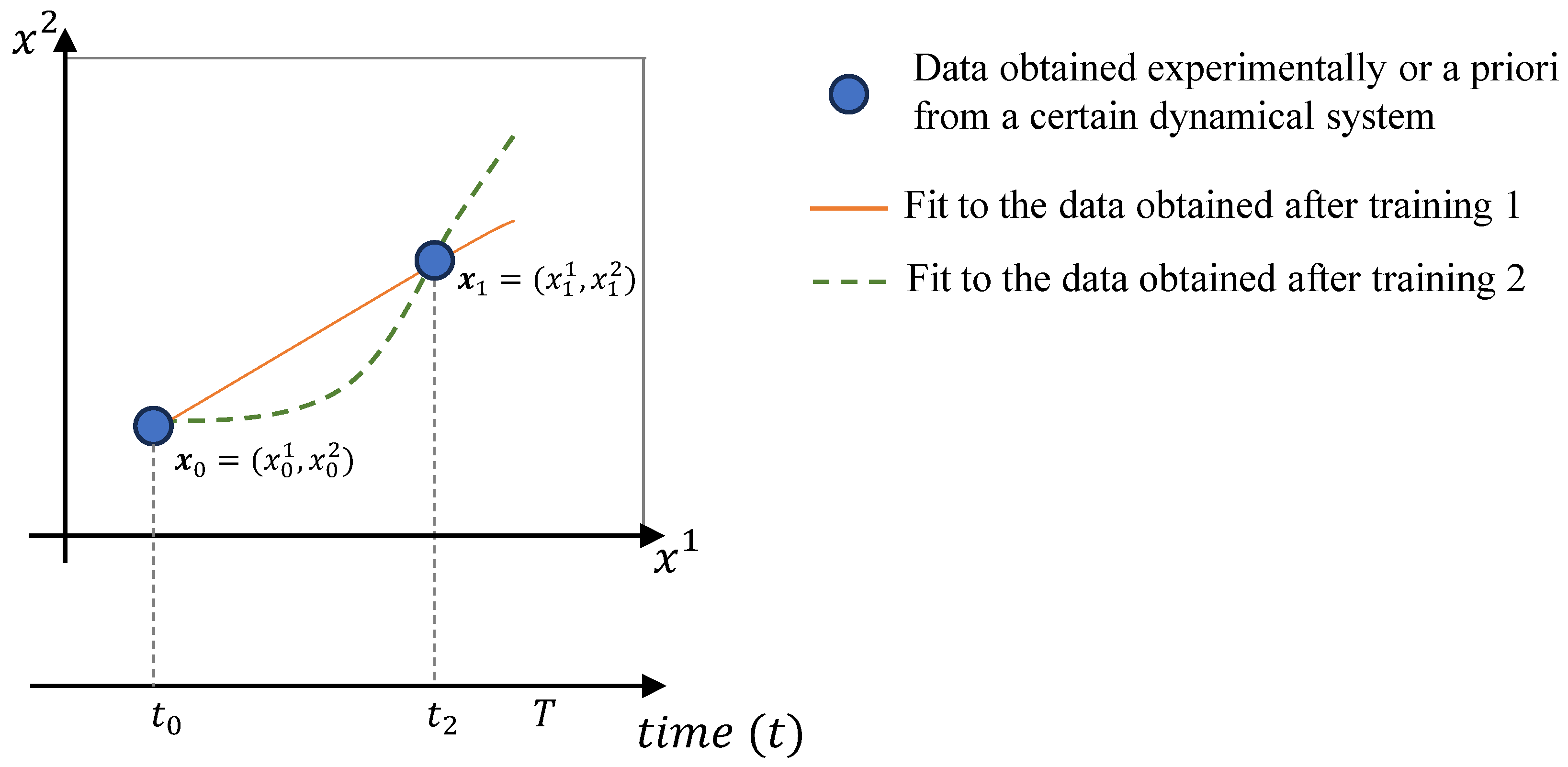
Figure 3.
Training loss evolution for Neural FDE when modelling for (a) , (b) , (c) and (d) initialisation (Loss (vertical axis) vs Number of Iterations (horizontal axis)).
Figure 3.
Training loss evolution for Neural FDE when modelling for (a) , (b) , (c) and (d) initialisation (Loss (vertical axis) vs Number of Iterations (horizontal axis)).
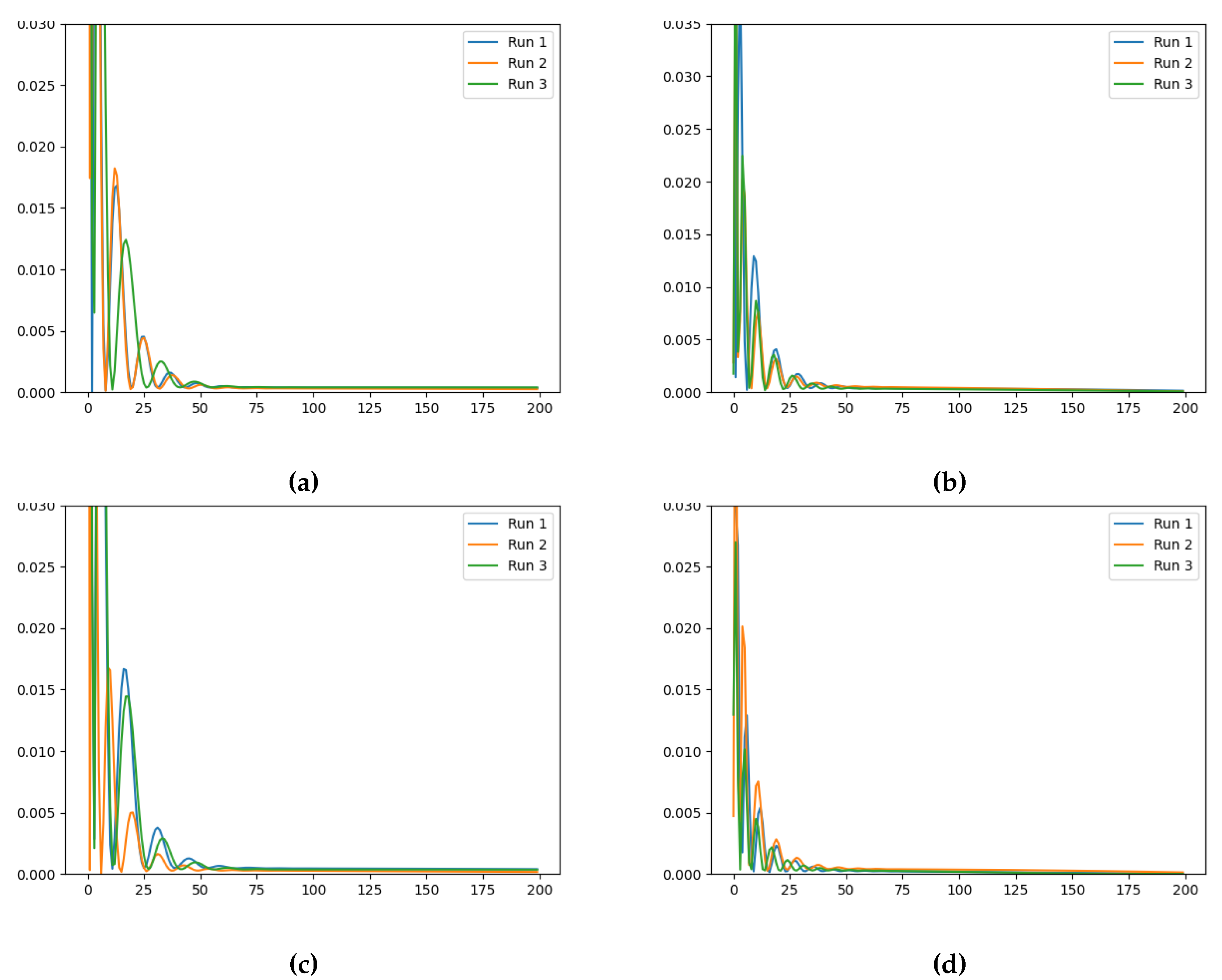
Figure 4.
Evolution of along the iterations. Case for (a) , (b) , (c) and (d) initialisation ( (vertical axis) vs Number of Iterations (horizontal axis)).
Figure 4.
Evolution of along the iterations. Case for (a) , (b) , (c) and (d) initialisation ( (vertical axis) vs Number of Iterations (horizontal axis)).
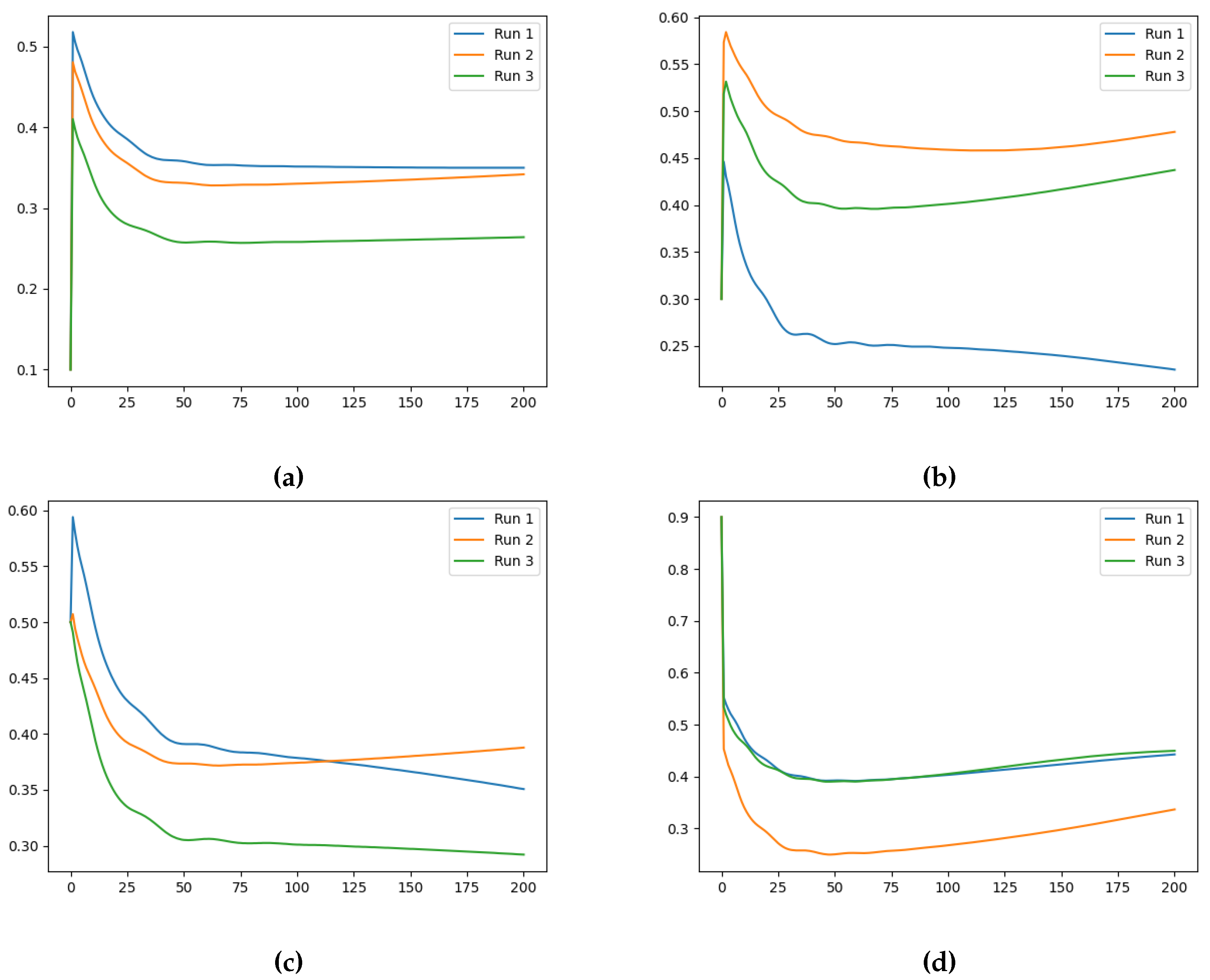
Figure 5.
Training loss evolution of the Neural FDE when modelling for a fixed (a) , (b) , (c) and (d) (Loss (vertical axis) vs Number of Iterations (horizontal axis)).
Figure 5.
Training loss evolution of the Neural FDE when modelling for a fixed (a) , (b) , (c) and (d) (Loss (vertical axis) vs Number of Iterations (horizontal axis)).
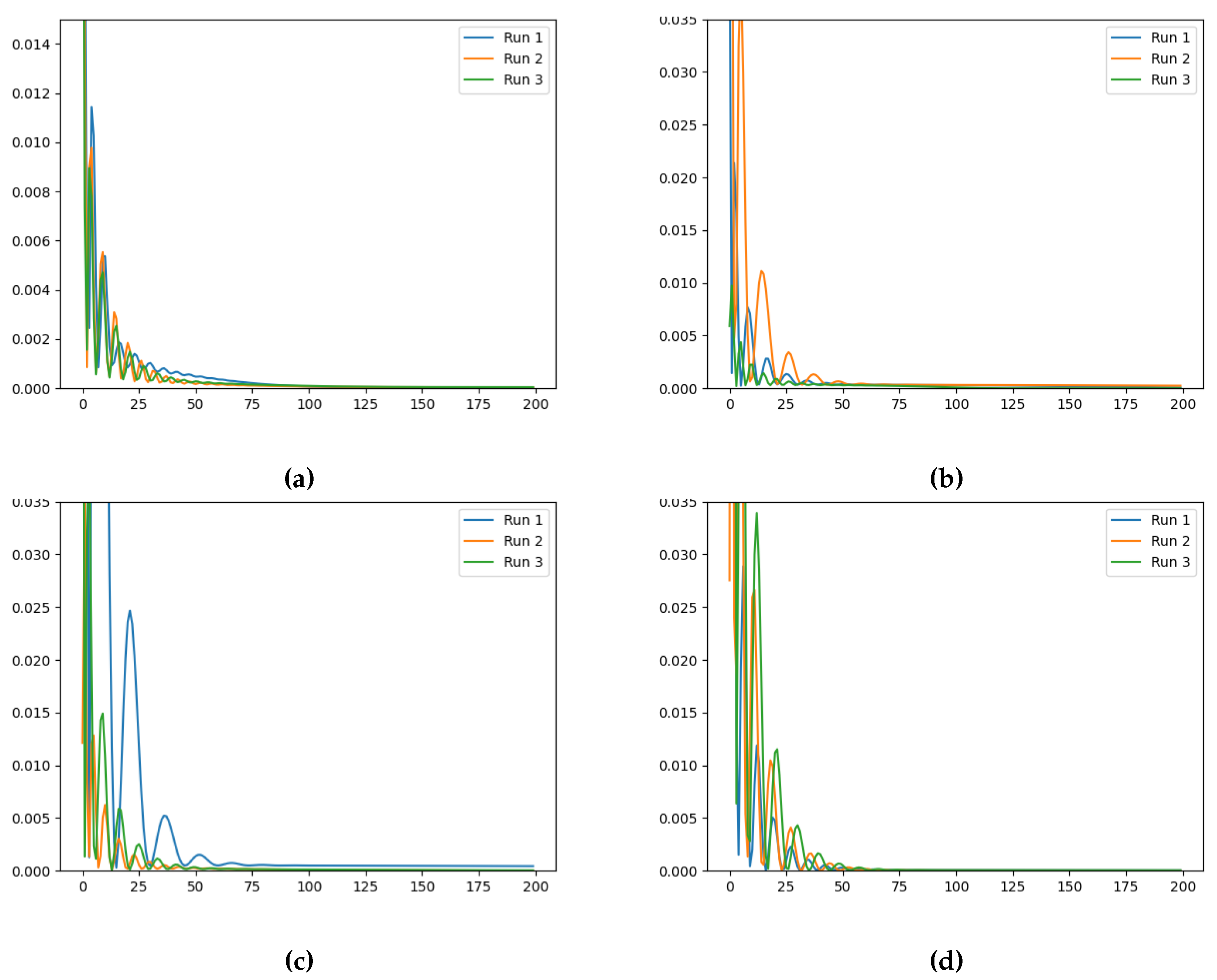
Figure 6.
Training loss evolution of the Neural FDE when modelling for a fixed (a) , (b) , (c) and (d) (Loss (vertical axis) vs Number of Iterations (horizontal axis)).
Figure 6.
Training loss evolution of the Neural FDE when modelling for a fixed (a) , (b) , (c) and (d) (Loss (vertical axis) vs Number of Iterations (horizontal axis)).
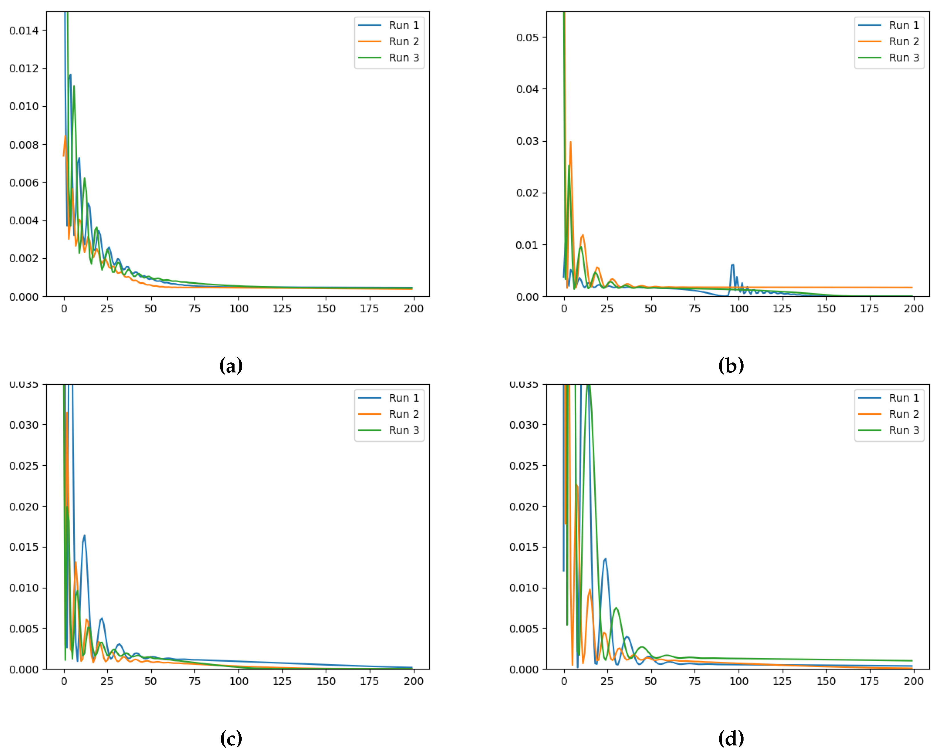
Figure 7.
Training loss evolution of the Neural FDE when modelling for a fixed (a) , (b) , (c) and (d) (Loss (vertical axis) vs Number of Iterations (horizontal axis)).
Figure 7.
Training loss evolution of the Neural FDE when modelling for a fixed (a) , (b) , (c) and (d) (Loss (vertical axis) vs Number of Iterations (horizontal axis)).
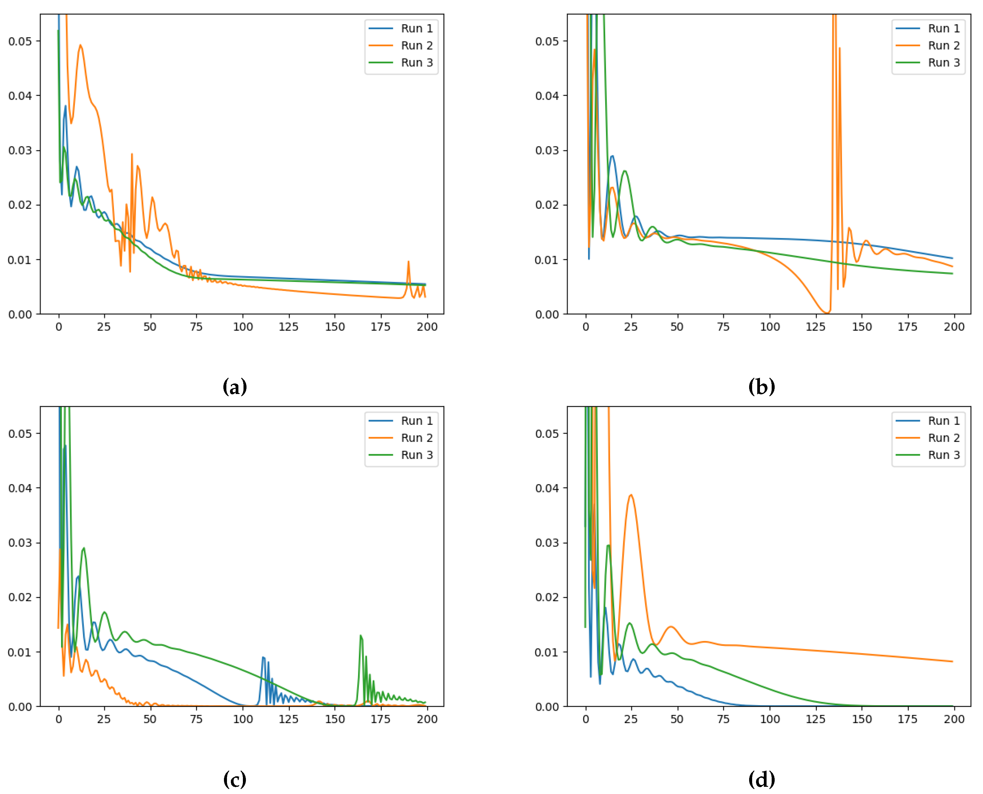

Table 1.
Learned and training loss obtained for three runs of a Neural FDE model, considering different initialisations. Case .
Table 1.
Learned and training loss obtained for three runs of a Neural FDE model, considering different initialisations. Case .
| Initialisation | Learnt | Training Loss |
|---|---|---|
| 0.1 | 0.3498|0.3417|0.2639 | 3.60E-04|2.50E-04|3.89E-04 |
| 0.3 | 0.2248|0.478|0.4374 | 1.44E-04|8.40E-05|8.00E-05 |
| 0.5 | 0.3507|0.3878|0.2921 | 3.90E-04|1.67E-04|3.53E-04 |
| 0.99 | 0.4427|0.3367|0.4497 | 3.50E-05|1.30E-04|6.00E-06 |
Table 2.
Learned and training loss obtained for three runs of a Neural FDE model, considering different initialisations. Case .
Table 2.
Learned and training loss obtained for three runs of a Neural FDE model, considering different initialisations. Case .
| Initialisation | Learnt | Training Loss |
|---|---|---|
| 0.1 | 0.2927|0.4924|0.4873 | 1.36E-03|2.00E-06|5.20E-05 |
| 0.3 | 0.455|0.4744|0.3923 | 3.00E-06|6.00E-06|9.52E-04 |
| 0.5 | 0.5162|0.2955|0.468 | 6.76E-04|1.02E-03|3.17E-04 |
| 0.99 | 0.4191|0.5372|0.503 | 9.20E-05|5.00E-06|3.00E-06 |
Table 3.
Learned and training loss obtained for three runs of a Neural FDE model, considering different initialisations. Case .
Table 3.
Learned and training loss obtained for three runs of a Neural FDE model, considering different initialisations. Case .
| Initialisation | Learnt | Training Loss |
|---|---|---|
| 0.1 | 0.6216|0.5173|0.5407 | 7.00E-06|3.11E-03|1.26E-03 |
| 0.3 | 0.2738|0.5429|0.5364 | 7.48E-03|4.00E-06|8.73E-04 |
| 0.5 | 0.518|0.5586|0.5876 | 5.00E-06|1.00E-05|8.00E-06 |
| 0.99 | 0.5652|0.5141|0.5666 | 1.60E-05|4.92E-04|1.00E-05 |
Table 4.
Final training loss for three runs of the Neural FDE (fixed ). Case .
| Fixed | Training Loss |
|---|---|
| 0.1 | 3.50E-05|4.50E-05|4.90E-05 |
| 0.3 | 7.70E-05|2.44E-04|1.00E-06 |
| 0.5 | 4.36E-04|1.00E-05|4.30E-05 |
| 0.99 | 3.60E-05|2.10E-05|4.00E-05 |
Table 5.
Final training loss for three runs of the Neural FDE (fixed ). Case .
| Fixed | Training Loss |
|---|---|
| 0.1 | 4.53E-04|3.78E-04|4.27E-04 |
| 0.3 | 1.00E-06|1.70E-03|3.00E-06 |
| 0.5 | 1.70E-04|3.00E-06|4.00E-06 |
| 0.99 | 3.60E-04|6.70E-05|1.00E-03 |
Table 6.
Final training loss for three runs of the Neural FDE (fixed ). Case .
| Fixed | Training Loss |
|---|---|
| 0.1 | 5.44E-03|3.10E-03|5.22E-03 |
| 0.3 | 1.02E-02|8.68E-03|7.37E-03 |
| 0.5 | 4.00E-06|6.10E-05|7.05E-04 |
| 0.99 | 2.00E-06|8.18E-03|1.00E-08 |
Table 7.
Number of iterations needed to achieve a final training loss of 1E-05, with the different fixed values, when modelling .
Table 7.
Number of iterations needed to achieve a final training loss of 1E-05, with the different fixed values, when modelling .
| Fixed | Number of Iterations |
|---|---|
| 0.1 | 791 ± 90 |
| 0.3 | 934 ± 76 |
| 0.5 | 265 ± 2 |
| 0.99 | 1035 ± 462 |
Table 8.
Number of iterations needed to achieve a final training loss of 1E-05, with the different fixed values, when modelling .
Table 8.
Number of iterations needed to achieve a final training loss of 1E-05, with the different fixed values, when modelling .
| Fixed | Number of Iterations |
|---|---|
| 0.1 | 2837 ± 1697 |
| 0.3 | 4659 ± 1114 |
| 0.5 | 193 ± 47 |
| 0.99 | 3255 ± 2003 |
Table 9.
Number of iterations needed to achieve a final training loss of 1E-05, with the different fixed values, when modelling .
Table 9.
Number of iterations needed to achieve a final training loss of 1E-05, with the different fixed values, when modelling .
| Fixed | Number of Iterations |
|---|---|
| 0.1 | -* |
| 0.3 | 3119 ± 460 |
| 0.5 | 128 ± 28 |
| 0.99 | 240 ± 137 |
* In 10000 iterations it was not possible to achieve a final training loss of 1e-05 in both runs. However the final training loss was 1.2e-05.
Disclaimer/Publisher’s Note: The statements, opinions and data contained in all publications are solely those of the individual author(s) and contributor(s) and not of MDPI and/or the editor(s). MDPI and/or the editor(s) disclaim responsibility for any injury to people or property resulting from any ideas, methods, instructions or products referred to in the content. |
© 2024 by the authors. Licensee MDPI, Basel, Switzerland. This article is an open access article distributed under the terms and conditions of the Creative Commons Attribution (CC BY) license (http://creativecommons.org/licenses/by/4.0/).
Copyright: This open access article is published under a Creative Commons CC BY 4.0 license, which permit the free download, distribution, and reuse, provided that the author and preprint are cited in any reuse.