Understanding Risk Factors of Recurrent Anxiety Symptomatology in an Older Population with Mild to Severe Depressive Symptoms: A Bayesian Approach

Anxiety in older individuals is understudied despite its prevalence. Investigating its occurrence can be challenging, yet understanding the factors influencing its recurrence is important for improved management. This study aimed to model the recurrence of anxiety symptomatology in an older population within a five-month timeframe. Data included baseline socio-demographic and general health information for older adults aged 60 years or older with at least mild depressive symptoms. A Bayesian network model explored the relationship between baseline data and recurrent anxiety symptomatology. Model evaluation employed the Area Under the Receiver Operating Characteristic Curve (AUC). The Bayesian model was also compared to three machine learning models. The model achieved an AUC of 0.821 on the test data, using a threshold of 0.367. This result surpassed both the Logistic Regression and XGBoost models, but slightly behind SGDClassifier. Key factors associated with recurrence of anxiety symptomatology were: “Not being able to stop or control worrying”; “Becoming easily annoyed or irritable”; “Trouble relaxing”; and “depressive symptomatology severity”. The model demonstrated generalisation abilities and outperformed some machine learning models while being less complex and more explainable. These findings indicate a prioritised sequence of predictors to identify individuals most likely to experience recurrent anxiety symptomatology.

Keywords:

Subject: Computer Science and Mathematics - Artificial Intelligence and Machine Learning

1. Introduction

The concepts of anxiety recurrence and remission are crucial for understanding the nature of anxiety disorder. Anxiety recurrence is defined as the re-emergence of symptoms after a period of remission [1]. Remission is achieved when the patient returns to their usual self, possibly presenting mild or no residual symptoms of the anxiety disorder [2].

A study by Scholten et al., indicated that 23.5% of individuals with remitted anxiety will experience a recurrence of anxiety within two years [3]. This study highlights that recurrent anxiety presents an obstacle to individual well-being and societal growth. Despite advancements in understanding its relationship with predictors, recurrent anxiety continues to pose significant challenges for those who suffer from it.

Minimising recurrent anxiety is crucial not only for individuals but also for society, as anxiety symptomatology affect well-being, social relationships, and work productivity [4], resulting in economic burden including increased treatment costs [5]. To prevent recurrent anxiety, it is essential to identify those at highest risk and understand the most important predictors. This understanding is crucial so that relapse prevention efforts can be targeted towards those patients most in need [1].

Several studies analysed the relationships between anxiety recurrence and its predictors. For instance, general measures of anxiety, fearfulness, work and home disability [6], comorbid generalised anxiety and depression [2], worsening psychosocial impairment [7], discontinuation of antidepressant medication [8], fear of anxiety-related sensations and neuroticism [9] have been identified as predictors of anxiety symptomatology recurrence. However, none of these studies have specifically focused on the older population.

The growing concern about anxiety symptomatology in the older population is not only due to its high level of recurrence but also due to the possible influence it may have on the incidence and prognosis of other health problems typical of aging, such as disability and depression [10]. A 9-year prospective study involving older adults aged 55 to 85 at baseline demonstrated that the presence of more anxiety symptoms at baseline predicted the onset of an anxiety symptomatology, emphasising the importance of targeting individuals displaying more early symptoms but not meeting the specific diagnostic criteria for anxiety symptomatology [11].

In such a context, the application of machine learning (ML) can be useful as it may result in understanding the relationship between factors associated with anxiety. One particularly suitable approach is to employ Bayesian networks (BNs) as they provide both explainability and a measure of prediction uncertainty. BNs represent a graph-based method that captures interactions among variables, thereby enhancing explainability of their mutual influences [12]. Owing to their probabilistic nature, BNs inherently provide quantitative information regarding the uncertainty linked with predictions.

The objective of this study is to use BNs to model the recurrence of anxiety symptomatology within a five-month timeframe in a population aged 60 years and older with mild to severe depressive symptoms and to investigate the key factors that have an impact on its occurrence.

2. Materials and Methods

2.1. Data

We utilised a dataset from randomised controlled trials assessing the effectiveness of mobile messaging psychosocial interventions for depression and subthreshold depression among older adults in resource-limited settings in Brazil [13]. Specifically, we focused on the groups that did not receive the psychosocial interventions, which comprised two subgroups: one with 305 individuals identified with depressive symptomatology (9-item Patient Health Questionnaire (PHQ-9) scores≥ 10) and another with 231 individuals experiencing subthreshold depressive symptomatology (9-item Patient Health Questionnaire (PHQ-9) scores between 5 and 9, inclusive).

The data included baseline information on socio-demographics (gender, age, marital status, race), self-reported general health (hypertension, diabetes, depression, balance), depressive symptomatology (PHQ-9), anxiety symptomatology (GAD-7), loneliness (3-item UCLA), health-related quality of life (EQ-5D-5L), and capability well-being (ICECAP-O).

Additionally, the dataset provided information on two follow-up periods: the first at three months after receiving a single message (follow-up 1) and the second at five months after baseline (follow-up 2). For these follow-ups, the only data included were related to depression (PHQ-9) and anxiety (GAD-7).

2.2. Outcome

In this study, an individual was considered to have recurrent anxiety symptomatology if they had a total score of 10 or higher on the GAD-7 questionnaire in any of the following scenarios: a) at baseline and follow-up 1; b) at baseline and follow-up 2; c) at baseline, follow-up 1 and follow-up 2.

Table A1 in the supplementary material summarises the socio-demographic and health-related characteristics of this cohort.

2.3. Bayesian Network Model

To comprehend the relationships between the baseline data and our outcome, we developed a Bayesian network model. A Bayesian Network is a directed acyclic graph comprising nodes and edges, utilised to construct an approximation of the joint probability distribution over all variables and the outcome of interest. This joint probability distribution provides all necessary information for making probabilistic inferences on one variable given knowledge of the other variables in the distribution. Nodes represent variables, while directed edges, depicted by arrows, elucidate relationships among these variables [14].

In our approach, we learned the BN from data [15,16]. We utilised a bootstrap approach [17] to generate 1,000 samples of the BN using a constraint-based algorithm, named Incremental Association Markov Blanket (IAMB) [18] . The IAMB algorithm effectively constructs Bayesian networks by incrementally including variables based on mutual information [19]. The latter which quantifies the statistical relationship between variables. This approach helps to identify relevant variables and construct a network that precisely represents the relationships found in the data.

A bootstrap approach ensures that the results are robust and helps minimise false patterns. This method outputs a summary table, illustrated in Table 1, that shows pairs of variables (called "features") and their relationships. The first two columns, "From" and "To," show the features associated with the outcome. The last two columns, "Strength" and "Direction," indicate the likelihood of a connection between the pairs and the direction of this connection. This process helps us understand which variables are related to the outcome, how strong their relationships are, and the direction of these relationships [20].

We only selected feature pairs where our outcome was present in either the "From" column or the "To" column. This selection was made because we are specifically interested in understanding the relationship between the outcome and the features at baseline. Additionally, we filtered only those directions with a probability greater than 50% and then ordered the summary table in descending order based on strength.

Next, we began constructing the first BN using only the first row of the table. As depicted in Table 1, this initial BN would consist of two nodes, with the "feature 1" node having an arrow pointing towards the "outcome" node (Figure 1 (A)). We then proceeded to build another BN using the first two rows. In this case, our outcome node receives arrows from both the "feature 1" and "feature 2" nodes, as illustrated in Figure 1 (B). We continued this process until all the connections from the bootstrap output had been used.

For each Bayesian network defined by the incremental addition of nodes ordered by strength, we computed the conditional probability distributions (CPD) associated with each node. This process, known as parameter learning, involves applying the Bayesian method [21]. Next, predictions for the outcome were made using exact inference [14], where the posterior probability is calculated based on a set of events. These events consist of all possible values of the nodes connected to our outcome.

Specifically, for cases (A), (B), and (C) in Figure 1, the joint probability distributions can be described by equations 1, 2, and 3, respectively.

P_{A} = P (f 1) . P (o u t c o m e | f 1)

(1)

P_{B} = P (f 1) . P (f 2) . P (o u t c o m e | f 1, f 2)

(2)

P_{C} = P (f 1) . P (f 2) . P (o u t c o m e | f 1, f 2) . P (f 3 | o u t c o m e)

(3)

where

P (f 1)

P (f 2)

P (f 3)

are the probability distributions of feature 1, 2 and 3.

P (o u t c o m e ∣ f 1)

represents the conditional probability distribution of the outcome given feature 1.

P (o u t c o m e ∣ f 1, f 2)

denotes the conditional probability distribution of the outcome given feature 1 and 2, and

P (f 3 ∣ o u t c o m e)

describes the conditional probability distribution of the feature 3 given the outcome.

We define features 1 and 2 as “parent” node of the “child” node outcome, while feature 3 is the “child” of its “parent” node outcome. Therefore, we can generalise the joint probability distribution for all other Bayesian network structures as shown in equation 4.

P (X_{1}, . . ., X_{n}) = \prod_{i = 1}^{n} P (X_{i} | P_{a} (X_{i}))

(4)

where

P a (X_{i})

denotes the parent of node

X_{i}

. The conditional probability for a node without parents is simply its prior probability

P (X_{i})

To develop the Bayesian Network model, we utilised the bnlearn package in R [22].

2.4. Model Evaluation and Inference

To rigorously evaluate our data-driven approach statistically, for each BN constructed as explained in the previous section, we employed repeated cross-validation with four folds, repeated 25 times using different random samples from the training data. In each of the 25 iterations, the dataset was divided into subsets, allowing the models to be trained on three folds and validated on the remaining fold. This process was conducted solely with the training data, which represents 70% of our total dataset to avoid any bias when evaluating the performance of the model on the unseen test data.

For each fold, using the predictions described in the previous section, we recorded the Area Under the receiver operating Characteristic curve (AUC), F1-score, and the threshold that maximised both sensitivity and specificity simultaneously, as determined by Youden’s index, in both the training folds (three folds) and the validation fold (one fold).

Then, we selected the BN that achieved the highest AUC value in the validation part to be tested on the remaining 30% of the data that had not been used during training. Using the BN that maximises the AUC, we learned the parameters on the entire training dataset, enabling us to generate new predictions for the test data using exact inference and the optimal threshold identified in the repeated cross-validation. Additionally, we calculated AUC and F1-score values on the test data for comparison with the cross-validation results.

Utilising the chosen BN and the learned parameters, we proceeded with an inference analysis by calculating the conditional probability tables of our outcome given the features individually. Moreover, we investigated the combinations of the features, assessing how their different values would collectively impact the outcome. We then analysed the individual contributions of features and also their interactions, elucidating potential synergistic or antagonistic effects on the outcome variable. This analysis was conducted by calculating probabilities, marginalising the selected features in each scenario.

2.5. Machine Learning Models Comparison

The Bayesian network model applied in this study was compared with three other models: Logistic Regression, the SGDClassifier [23], and XGBoost [24]. To ensure a fair comparison, we maintained identical splits of training and testing data across all four models.

We used Recursive Feature Elimination with Cross Validation (RFECV) to select the features for developing the three models. RFECV [25] is a feature selection method that iteratively eliminates the least important features from the dataset, while evaluating the model’s performance through cross-validation. This process uses a supervised learning estimator that provides information regarding feature importance. In this study, we used Logistic Regression as the estimator. After selecting the features, we used the same selected features for all three models.

It is common practice to fine-tune the parameters when developing a model, a process known as hyperparameter optimisation. This typically enhances the model’s performance. To fine-tune the hyperparameters and evaluate the model’s performance in a robust and unbiased manner, we applied nested cross-validation [26]. Nested cross-validation involves two main loops: an outer loop and an inner loop. In the outer loop, the dataset is divided into multiple folds. In each iteration of the outer loop, one fold is reserved as the test set, and the remaining folds are used as the training set. The outer loop is dedicated to evaluating the model.

In the inner loop, nested within the outer loop, hyperparameter tuning is performed. Here, the training set is further divided into folds, with one fold held out as a validation set, while the rest are used for training. Multiple models are trained and evaluated within this loop to find the best-performing set of hyperparameters.

After the inner loop completes, the set of hyperparameters that provided the best performance on the training folds is used on the test dataset reserved in the outer loop. The best performance is usually measured by maximising a defined metric, such as AUC or F1-score. The performance metrics obtained from each iteration of the outer loop are summarised to provide an overall assessment of the model’s performance.

In this study, we used nested cross-validation with four folds for both the inner and outer loops and 25 repetitions, resulting in 100 evaluations, similar to the repeated cross-validation used in the Bayesian network model. To fine-tune the hyperparameters, we employed Bayesian hyperparameter optimisation maximising the AUC metric [27].

Furthermore, we recorded the AUC metric, including the minimum, mean, maximum, and standard deviation from the outer loop iterations. Next, we selected the hyperparameters that resulted in the highest AUC value across the 100 evaluations and fitted the models with these hyperparameter settings on the test data.

Finally, we compared the AUC metrics of Logistic Regression, Stochastic Gradient Descent Classifier, and XGBoost with the AUC metric of the Bayesian network model.

3. Results

3.1. Data Processing

First, the data were filtered to ensure complete information on the GAD-7. We deleted 71 cases where information for the GAD-7 questionnaire was missing. This was because the study was designed to initially screen the GAD1 and GAD2 questions. If their sum was greater than or equal to 1, the remaining five questions were assessed; otherwise, these values were missing.

After the initial filtering, the descriptive analysis identified six features with more than 25% of the cases missing: “hypertensioncontrolled,” “diabetescontrolled,” "hypertensiontreatment," "diabetestreatment," "depressiontreatment," and "falls." However, when we correlated these six variables with other features, it was possible to infer the missing values.

For “hypertensioncontrolled” and “diabetescontrolled,” the missing cases were 99% correlated with not having hypertension and diabetes, respectively. Therefore, we filled the missing values for both features with “yes,” based on the assumption that if a participant does not have hypertension or diabetes, their condition is controlled.

For "hypertensiontreatment," "diabetestreatment," "depressiontreatment," and “falls,” the missing cases were 100% correlated with not having hypertension, diabetes, depression, and balance problems, respectively. Thus, we filled these missing values with “no,” assuming that if a participant does not have the condition, they do not require treatment for it.

After filling in these missing values, there were still 5% of values missing randomly, affecting 14 individuals, who were consequently dropped from the analysis.

3.2. Bayesian Network Construction

The results of the bootstrap are illustrated in Table 2, showing nine connections between features and the outcome. They include "gad6" (Becoming easily annoyed or irritable), "gad2" (Not being able to stop or control worrying), "Depression group" (four PHQ-9 score groups: 5-9, 10-14, 15-19, 20 or above), "gad4" (Trouble relaxing), "ucla3" (How often one feels isolated from others), "gad1" (Feeling nervous, anxious, or on edge), "ucla1" (Lack of company), “phq5” (Poor appetite or overeating), and “depression” (Have you been diagnosed with depression).

These nine connections are all directly connected to the outcome and appeared at least once in the 1,000 bootstrap samples used while building the Bayesian Network as discussed in Section 2.3.

As explained in Section 2.3, we constructed nine different Bayesian Networks. We began with the first BN, which had two nodes, with a directed arrow from our outcome “Recurrent anxiety” to "gad6". Next, we added the node "gad2" to the “Recurrent anxiety” node, maintaining the connection used in the first BN. Then, we incremented from BN number 3 to number 9 by adding nodes according to Table 2. All nine constructed BNs can be seen in Appendix A Figure A1.

Figure 2 displays the average AUC values from 100 evaluations on repeated cross-validation versus the nine different BNs constructed from the bootstrap. Figure 2 shows that the AUC consistently increases for the training folds. However, for the validation folds, there is a peak when the number of features is four, indicating that the BN with four features performs best. This result suggests it has the highest potential for strong performance and effective generalisation among all nine possible BNs.

3.3. Evaluation of the Model

Table 3 and Table 4 provide additional details regarding the AUC and F-1 score, respectively. We included the mean of the 100 evaluations from the training folds in the repeated cross-validation, as well as the minimum, mean, maximum, and standard deviation of the validation folds across all 100 evaluations. With a mean AUC of 0.836 and an F1-score of 0.765, the BN with four features was chosen for evaluation on the test data. This selection was based on the highest mean AUC achieved on the validation folds.

Due to the small size of the dataset (308 observations on training data), a wide range of AUC values is observed for the chosen model (see Table 3) from 0.648 to 0.959, with a standard deviation of 0.056. Regarding the F1-score, we obtained minimum and maximum values of 0.538 and 0.918, respectively, and a standard deviation of 0.053 (Table 4) for the chosen model with four features.

The selected BN is depicted in Figure 3, where "Depression group" (Four PHQ-9 score groups: 5-9, 10-14, 15-19, 20 or above) and "gad4" (Trouble relaxing) have a direct arrow pointing to the outcome. Additionally, “gad6" (Becoming easily annoyed or irritable), "gad2" (Not being able to stop or control worrying) receive an arrow from the outcome.

3.4. Performance of the Model on Unseen Data

Table 5 displays the metric values for training, repeated cross-validation, and test data. It is important to note that the training values here differ from those in the training values in Table 3 and Table 4. This is because in Table 5, the whole training dataset is utilised, whereas in Table 3 and Table 4, it is the average of the 100 evaluations of the training folds. The threshold that resulted in the maximum Youden’s index was 0.367.

3.5. Inference

The conditional probability tables for each feature and the outcome are illustrated in Table A2–Table A5 of the Appendix A. These tables show that the features with more discriminatory power are "Not being able to stop or control worrying" (gad2) and "Becoming easily annoyed or irritable" (gad6). For instance, if an individual reports not being able to stop or control worrying nearly every day at baseline, the probability of reporting to have recurrent anxiety symptomatology is 0.752 (Table A2 of the Appendix A). Furthermore, from Table A3 of the Appendix A, if an individual reports to become easily annoyed nearly every day at baseline, the probability of reporting to have recurrent anxiety symptomatology is 0.745.

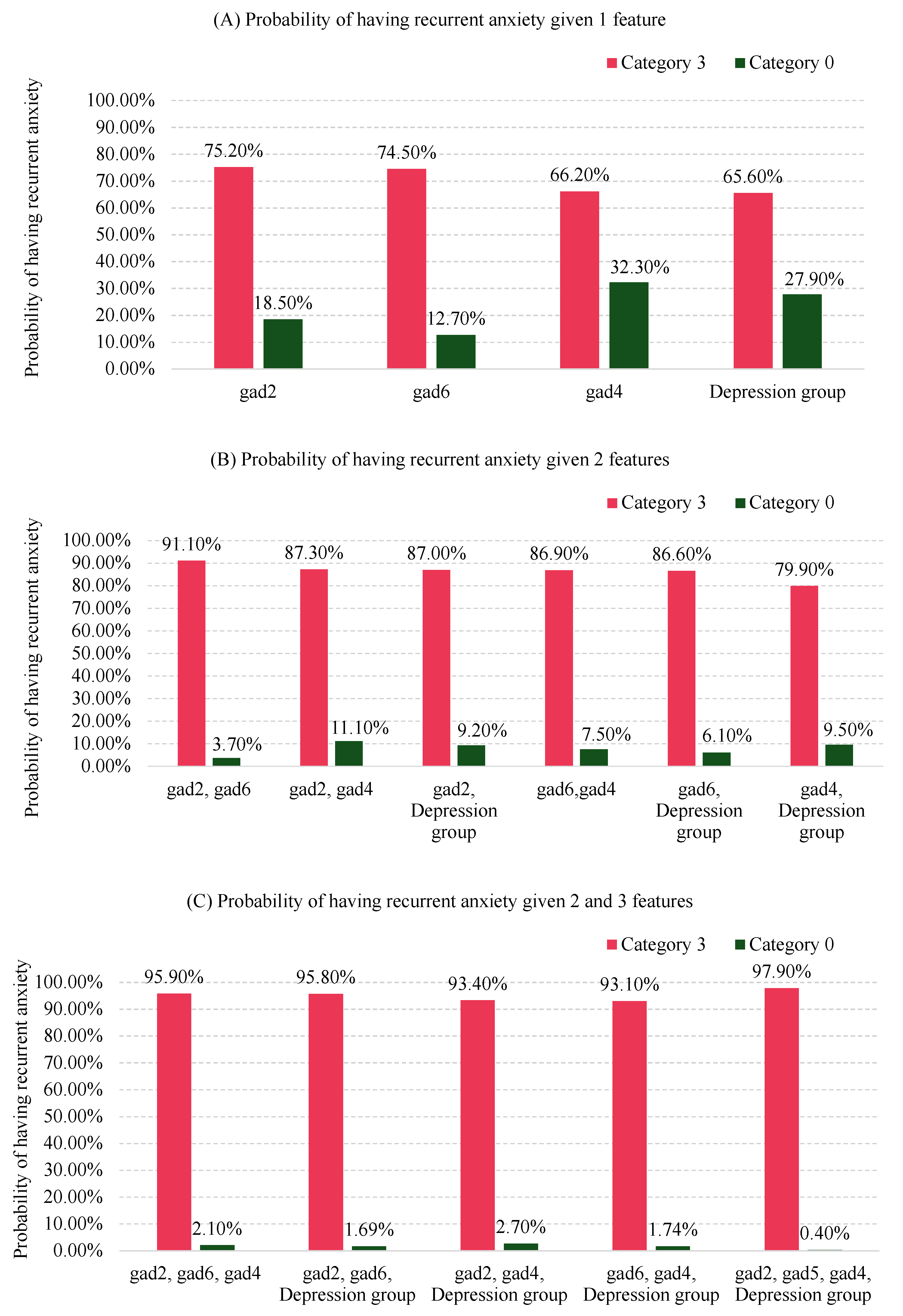
Although "Depression group" and "Trouble relaxing" (gad4) in isolation do not exhibit strong discriminatory performance similar to gad2 and gad6, Figure 4 demonstrates the significant contribution of these combined factors to the probability of recurrent anxiety symptomatology. For instance, the probability of having recurrent anxiety symptomatology is 0.752 if an individual reports "not being able to stop or control worrying" nearly every day (category "3" in Figure 3), compared with 0.185 if they report not worrying at all (category "0" in Figure 3), as shown in Figure 4 (A). When "not being able to stop or control worrying" (gad2) and "becoming easily annoyed or irritable" (gad6) are combined, the probability of recurrent anxiety symptomatology increases to 0.911 if both are reported nearly every day (category "3"). Conversely, this probability decreases to 0.037 if both are reported not at all (category "0") as shown in Figure 4 (B).

As more features are considered, the probabilities continue to change. For example, in Figure 4 (C), the probability of recurrent anxiety symptomatology reaches 0.979 if an individual reports "not being able to stop or control worrying" (gad2), "becoming easily annoyed or irritable" (gad6), and "trouble relaxing" (gad4) nearly every day (category "3"), and has a PHQ-9 score 20 or over (category "3" in Figure 3).

Conversely, the probability of having recurrent anxiety symptomatology is just 0.004 if an individual reports "not at all" (category "0") for gad2, gad6, and gad4, and falls into the category “0" for Depression group (PHQ-9 score between 5-9) as shown in Figure 4 (C).

Figure 4. Posterior probabilities scenarios of having recurrent anxiety symptomatology when combining the features of the BN model for 1 feature (A), 2 features (B) and 3 or 4 features (C). Category 3: Nearly every day for gad2, gad4, gad6, and a PHQ-9 score of 20 or higher for the depression group. Category 0: Not at all for gad2, gad4, gad6, and a PHQ-9 score between 5 and 9 for the depression group.

3.6. Comparison of the Models

Using RFECV, we selected ten features to develop the Logistic Regression, SGDClassifier and XGBoost models. The only feature in common with the Bayesian Network model was gad2. The remaining nine features are different and are described in Table A6 in the supplementary material.

Table 6 presents the AUC metric of the three models as well as the proposed BN model. The first four columns (Min, Mean, Max, SD) correspond to the 100 evaluations using nested cross-validation for the three models and the 100 evaluations of the repeated cross-validation in our approach. The last column indicates the AUC on the test data, which utilised the same data split for all four models, as discussed in Section 2.5.

From Table 6, it is observable that all three models outperformed the Bayesian network in terms of Mean AUC, with values of 0.897, 0.883, and 0.884 for Logistic Regression, SGDClassifier, and XGBoost, respectively, compared with 0.836 for the Bayesian network. Additionally, the standard deviations of the three models are lower than that of the Bayesian network, with values of 0.037, 0.050, and 0.039 for Logistic Regression, SGDClassifier, and XGBoost, respectively, compared with 0.056 for the Bayesian network.

However, upon evaluating the performance of the AUC metric on the test data, the Bayesian network exhibited an AUC of 0.821, while Logistic Regression, SGDClassifier and XGBoost, exhibited 0.814, 0.842, and 0.799 respectively. Given the cross-validation results on the training data, these test results should not be interpreted as meaning that the BN is superior, but they do show that the performance of the latter is not substantially inferior.

4. Discussion

The decision to use the BN was influenced by the observation that, after incorporating more than four features, the AUC on the validation set began to decline (Figure 2), while the AUC on the training set continued to increase. This suggests overfitting of the model. Overfitting occurs when a model performs well on the training data but poorly on the test data, indicating it may not generalise effectively to new, unseen data.

When we conducted predictions on the test data, we achieved an AUC of 0.821 and an F1-score of 0.743 (Table 5). These results closely align with those obtained through repeated cross-validation, falling within one standard deviation. This suggests that the model generalises well. It is expected that the training data yields higher values, as it is used to learn the parameters for making predictions. However, these values remain less than two standard deviations for F1-score. This further validates the robustness of the generalisation error estimated using repeated cross-validation with 100 evaluations.

4.1. Inference Analysis

One practical application provided by the analysis in Figure 4 is its usefulness in identifying individuals based on the three symptoms of anxiety and the level of depressive symptomatology severity—the four key factors relevant to recurrent anxiety symptomatology shown in Figure 3. This can help in developing specific interventions for these individuals.

If data and time are limited, clinicians should prioritise gathering information about gad2, as it has the highest probability of indicating recurrent anxiety symptomatology when the symptom occurs "nearly every day" (category 3 in Figure 4 (A). If constraints are less stringent, clinicians should prioritise information about both gad2 and gad6, as these combined have the highest probability of indicating recurrent anxiety symptomatology when both symptoms are in category 3 (Figure 4 (B)).

Next, information about gad4 should be prioritised, as combining this with gad2 and gad6 has the highest probability of indicating recurrent anxiety symptomatology when the symptom is in category 3 (Figure 4 (C)).

Finally, combining all three previous symptoms in category 3 with "Depression group" also in category 3 (PHQ score ≥ 20) increases the probability of having recurrent anxiety symptomatology to 97.9%. Conversely, having category 0 ("not at all") for gad2, gad6, and gad4, and a PHQ score between 5-9 for the depression group, results in a probability of 0.4% for recurrent anxiety symptomatology. This analysis suggests a prioritised order of importance for the features to focus on.

To gain a different perspective on the model, we analysed the test data for all individuals who had baseline values of 0 for gad2, gad6, and the Depression group. This indicates an absence of symptoms related to “Not being able to stop or control worrying,” “Becoming easily annoyed or irritable,” and a PHQ-9 score between 5-9. This analysis aimed to explore the impact of other features not selected by the BN model on the outcome.

We found five individuals out of 106 (5%) who met these criteria, and none of them presented recurrent anxiety symptomatology. For instance, one case experienced “Feeling nervous, anxious, or on edge” (gad1) for more than half the days and “Worrying too much about different things” (gad3) nearly every day at baseline, yet did not present recurrent disorder. Another participant experienced gad1 for more than half the days and “Feeling afraid, as if something awful might happen” (gad7) nearly every day at baseline, but also did not present recurrent anxiety symptomatology. Additionally, a third individual experienced gad1, gad3, and gad7 for more than half the days each, and similarly did not present recurrent anxiety symptomatology. This further suggests that the focus should be on the features identified by the BN model.

Although this study primarily focused on older individuals, the Depression group identified by our BN model is also recognised as a predictor of recurrent anxiety symptomatology, as demonstrated in another study [2], albeit in the general population.

4.2. Bayesian Network Model Comparison

The BN model underperformed compared to Logistic Regression, the SGDClassifier, and XGBoost. However, our approach offers some notable advantages. For instance, while all three models utilised 10 features for development, the BN model utilised only four. This results in a less complex model, and a reduced risk of overfitting, leading to improved generalisation on new, unseen data.

Furthermore, the BN model provides explainability, highlighting the most important features related to recurrent anxiety symptomatology and offering insights through probabilistic measures. These measures show the impact of increasing or decreasing the values of these features.

Another important point is that the BN model suggests a specific order of importance for the features. This indicates which key factors should be considered first to increase the likelihood of identifying individuals most likely to have recurrent anxiety symptomatology.

In Table 5, both Logistic Regression and XGBoost showed a smaller standard deviation compared with the BN model. However, the difference between the test data and the mean of the nested cross-validation exceeds two standard deviations. Additionally, although the SGDClassifier displayed a difference within one standard deviation between the test data and the mean of nested cross-validation, this difference remained higher than that observed in the BN model.

5. Conclusions

Using a Bayesian network, we aimed to understand the relationships of baseline data with the recurrence of anxiety symptomatology within five months. The model achieved an AUC of 0.821 and an F1-score of 0.743 on the test data.

We identified that "Not being able to stop or control worrying", "Becoming easily annoyed or irritable", and "Trouble relaxing", along with "depressive symptomatology severity" were the most important predictors for understanding recurrent anxiety symptomatology in this population.

Our analysis indicates a prioritised sequence of predictors to analyse for identifying individuals most likely to experience recurrent anxiety symptomatology. This sequence is as follows: "Not being able to stop or control worrying", "Becoming easily annoyed or irritable", "Trouble relaxing", "depressive symptomatology severity”.

The prioritised order of the predictors was ensured by testing all possible combinations on the optimal BN structure, extracting probabilities through marginalisation of each combination. Marginalisation is an useful approach for checking these combinations because it allows us to zoom out and focus on the overall scenarios, while also enabling us to examine more detailed aspects if needed.

6. Limitations

The features selected in the model demonstrated relevance and achieved good performance for this specific dataset, which comprises older individuals aged 60 and over with a PHQ-9 total score of at least 5. Nevertheless, it is noteworthy to acknowledge that in different populations, different factors may be seen as indicators of recurring anxiety.

Introducing more granular data could improve the model’s performance. Furthermore, our contention that the BN model provides clinicians with information to prioritise the treatment of specific symptoms would need to be tested using a suitable clinical trial.

Despite utilising a bootstrap approach during construction to enhance the chances of finding the optimal solution, we cannot guarantee optimality of the found network, especially given the small dataset size, which introduces considerable variability. There may be other network layouts that could potentially outperform this approach. For instance, including additional variables in this study may lead to better performance. However, this is not a limitation of the proposed methodology, but rather of the data available during the research.

Author Contributions

EM, MM, CAN, PV, MS conceived and designed the study. MM conducted the literature review regarding the psychology view. EM conducted the literature review, performed the machine learning analysis, and subsequently wrote the manuscript, which was reviewed by CN, RA, TJP, PV, MS. All authors contributed to and approved the final manuscript.

Funding

This publication has emanated from research supported in part by a grant from Science Foundation Ireland under Grant number 18/CRT/6049 (Eduardo Maekawa). Additionally, this study was funded by the Sao Paulo Research Foundation (process number 2017/50094 2) and the Joint Global Health Trials initiative, jointly funded by the Department of Health and Social Care (DHSC), the Foreign, Commonwealth & Development Office (FCDO), the Medical Research Council (MRC) and Wellcome (process number MR/R006229/1). FAPESP supported CAN (2018/19343-9) and (2022/05107-7), MM (2021/03849-3). MS is supported by CNPq-Brazil (307579/2019-0).

Institutional Review Board Statement

Ethical approval was obtained from the Ethics Committee of the Hospital das Clínicas da Faculdade de Medicina da Universidade de São Paulo (HCFMUSP) (CAPPesq, ref: 4.097.596 and CAPPesq, ref: 4.144.603). Additionally, the study was authorised by the Secretaria da Saúde do Município de Guarulhos. Verbal informed consent to participate in the study was requested from all participants.

Informed Consent Statement

Participants were informed that non-identifiable data would be used for publications prior to providing consent in both assessments. Informed consent materials are available from the corresponding author upon request.

Data Availability Statement

Study documentation and data will be made available upon request in accordance with data sharing conditions.

Conflicts of Interest

The authors declare that the research was conducted in the absence of any commercial or financial relationships that could be construed as a potential conflict of interest.

Abbreviations

The following abbreviations are used in this manuscript:

AUC	Area Under the Receiver Operating Characteristic Curve
ML	Machine Learning
BN	Bayesian network
IAMB	Incremental Association Markov Blanket
CPD	Conditional Probability Distributions
RFECV	Recursive Feature Elimination with Cross Validation

Appendix A

Figure A1. Incremental construction of the bayesian networks.

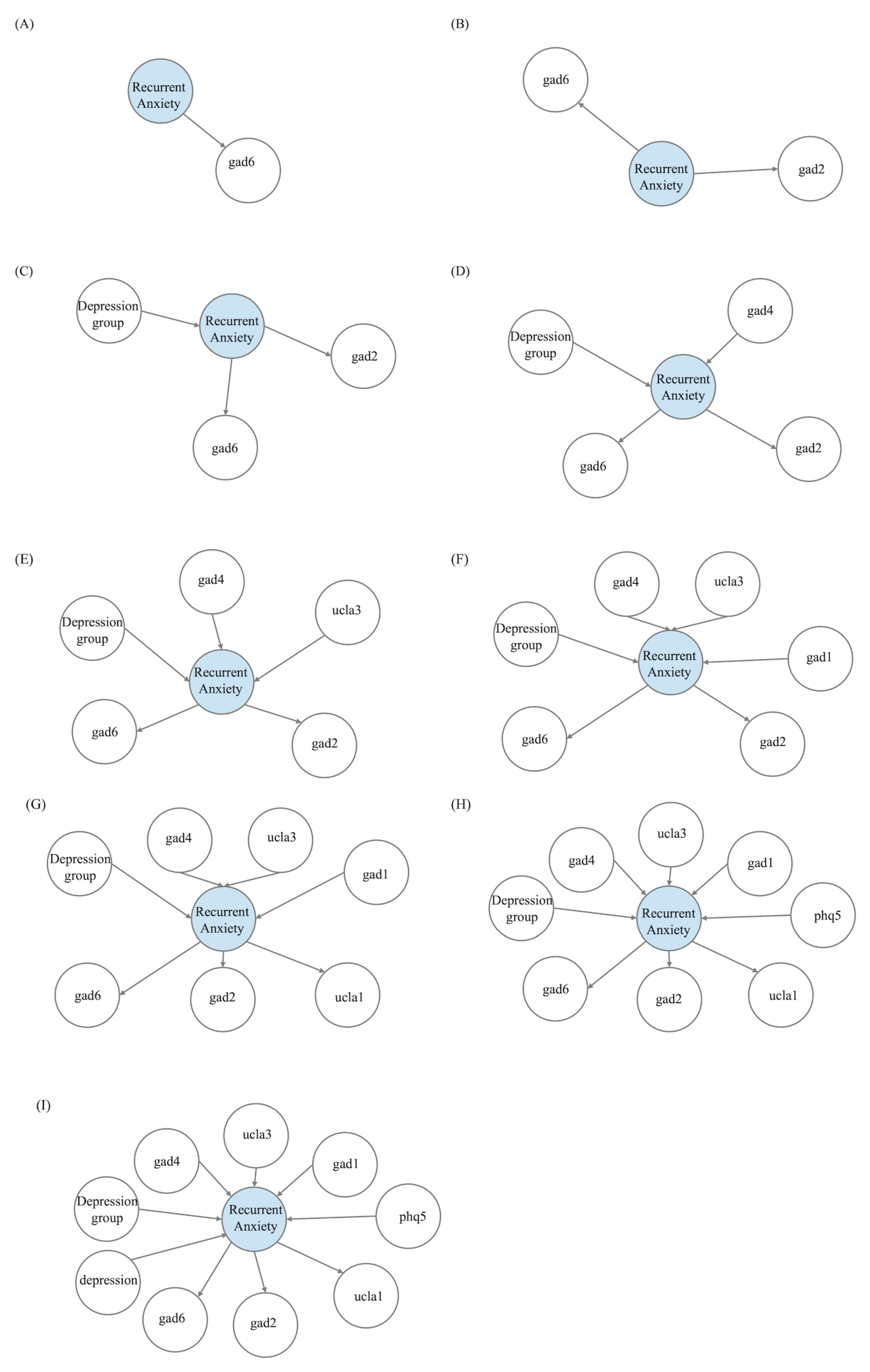
Table A1. Table of Characteristics

Feature	Range	N	% Recurrency of Anxiety
Gender	Female	263	0.494
	Male	112	0.402
Age group	70 year or over	112	0.518
	Between 60 and 69	243	0.469
Marital status	Divorced	68	0.397
	Married	212	0.491
	Single	29	0.552
	Widowed	66	0.424
Race	Asian	8	0.375
	Black	36	0.611
	Brown	159	0.421
	Native brazilian	3	0.333
	White	169	0.485
Depression group	PHQ-9 score: 10-14	87	0.494
	PHQ-9 score: 15-19	79	0.620
	PHQ-9 score: 20 or above	66	0.803
	PHQ-9 score: 5-9	143	0.210
Hypertension	No	106	0.396
	Yes	269	0.494
Diabetes	No	239	0.477
	Yes	136	0.449

Table A2. Conditional probability distribution – gad2: "Not being able to stop or control worrying"

	not at all	less than a week	more than half the days	nearly every day
No Anxiety	0.8152756	0.8121899	0.6355257	0.2476558
Anxiety	0.1847244	0.1878101	0.3644743	0.7523442

Table A3. Conditional probability distribution - gad6: "Becoming easily annoyed or irritable"

	not at all	less than a week	more than half the days	nearly every day
No Anxiety	0.8726873	0.7803838	0.3191136	0.254687
Anxiety	0.1273127	0.2196162	0.6808864	0.745313

Table A4. Conditional probability distribution – gad4: “Trouble relaxing”

	not at all	less than a week	more than half the days	nearly every day
No Anxiety	0.6774251	0.7721824	0.5187359	0.3384495
Anxiety	0.3225749	0.2278176	0.4812641	0.6615505

Table A5. Conditional probability distribution – Depression group

	PHQ-9: 5-9	PHQ-9: 10-14	PHQ-9: 15-19	PHQ-9: $\geq 20$
No Anxiety	0.7211609	0.5201635	0.3372896	0.3441699
Anxiety	0.2788391	0.4798365	0.6627104	0.6558301

Table A6. Features selected by the Recursive Feature Elimination with Cross-Validation

Features	Description	Range of the values
tobacco	Do you currently smoke?	0: No
		1: Yes
phq5	Over the last 2 weeks,	0: Not at all
	how often have you been	1: Several days
	bothered by Poor appetite	2: More than half the days
	or overeating	3: Nearly every day
gad2	Over the last 2 weeks,	0: Not at all
	how often have you been	1: Several days
	bothered by Not being able	2: More than half the days
	to stop or control worrying	3: Nearly every day
gad5	Over the last 2 weeks,	0: Not at all
	how often have you been	1: Several days
	bothered by Being so restless	2: More than half the days
	that it is hard to sit still	3: Nearly every day
gad3	Over the last 2 weeks,	0: Not at all
	how often have you been	1: Several days
	bothered by Worrying so	2: More than half the days
	much about different things	3: Nearly every day
ucla1	How often do you	1: Hardly ever
	feel that you lack	2: Some of the time
	companionship	3: Often
depression	Are you currently receiving	0: No
treatment	any treatment for depression	1: Yes
hypertension	Have you been diagnosed	0: No
	with hypertesion?	1: Yes
icecap4	Enjoyment and pleasure	1: I can’t have any enjoyment and pleasure
		2: I can have a little enjoyment and pleasure
		3: I can have a lot of enjoyment and pleasure
		4: I can have all the enjoyment and pleasure
balance	Do you have balance	0: No
	disorder?	1: Yes

References

Taylor, J.H.; Jakubovski, E.; Bloch, M.H. Predictors of anxiety recurrence in the Coordinated Anxiety Learning and Management (CALM) trial. Journal of Psychiatric Research 2015, 65, 154–165. [CrossRef]
Bruce, S.E.; Yonkers, K.A.; Otto, M.W.; Eisen, J.L.; Weisberg, R.B.; Pagano, M.; Shea, M.T.; Keller, M.B. Influence of psychiatric comorbidity on recovery and recurrence in generalized anxiety disorder, social phobia, and panic disorder: a 12-year prospective study. Am J Psychiatry 2005, 162, 1179–87. [CrossRef]
Scholten, W.D.; Batelaan, N.M.; van Balkom, A.J.L.M.; Wjh. Penninx, B.; Smit, J.H.; van Oppen, P. Recurrence of anxiety disorders and its predictors. Journal of Affective Disorders 2013, 147, 180–185. [CrossRef]
Alonso, J.; Angermeyer, M.C.; Bernert, S.; Bruffaerts, R.; Brugha, T.S.; Bryson, H.; de Girolamo, G.; Graaf, R.; Demyttenaere, K.; Gasquet, I.; et al. Disability and quality of life impact of mental disorders in Europe: results from the European Study of the Epidemiology of Mental Disorders (ESEMeD) project. Acta Psychiatr Scand Suppl 2004, pp. 38–46. [CrossRef]
Smit, F.; Cuijpers, P.; Oostenbrink, J.; Batelaan, N.; de Graaf, R.; Beekman, A. Costs of nine common mental disorders: implications for curative and preventive psychiatry. J Ment Health Policy Econ 2006, 9, 193–200.
Mavissakalian, M.R.; Guo, S. Early detection of relapse in panic disorder. Acta Psychiatr Scand 2004, 110, 393–9. [CrossRef]
Rodriguez, B.F.; Bruce, S.E.; Pagano, M.E.; Keller, M.B. Relationships among psychosocial functioning, diagnostic comorbidity, and the recurrence of generalized anxiety disorder, panic disorder, and major depression. J Anxiety Disord 2005, 19, 752–66. [CrossRef]
Donovan, M.R.; Glue, P.; Kolluri, S.; Emir, B. Comparative efficacy of antidepressants in preventing relapse in anxiety disorders — A meta-analysis. Journal of Affective Disorders 2010, 123, 9–16. [CrossRef]
Calkins, A.W.; Otto, M.W.; Cohen, L.S.; Soares, C.N.; Vitonis, A.F.; Hearon, B.A.; Harlow, B.L. Psychosocial predictors of the onset of anxiety disorders in women: results from a prospective 3-year longitudinal study. J Anxiety Disord 2009, 23, 1165–9. [CrossRef]
Wolitzky-Taylor, K.B.; Castriotta, N.; Lenze, E.J.; Stanley, M.A.; Craske, M.G. Anxiety disorders in older adults: a comprehensive review. Depress Anxiety 2010, 27, 190–211. [CrossRef]
Vink, D.; Aartsen, M.J.; Comijs, H.C.; Heymans, M.W.; Penninx, B.W.; Stek, M.L.; Deeg, D.J.; Beekman, A.T. Onset of anxiety and depression in the aging population: comparison of risk factors in a 9-year prospective study. Am J Geriatr Psychiatry 2009, 17, 642–52. [CrossRef]
Pearl, J. From Bayesian networks to causal networks. Mathematical Models for Handling Partial Knowledge in Artificial Intelligence 1995, pp. 157–182.
Scazufca, M.; Nakamura, C.A.; Seward, N.; Didone, T.V.N.; Moretti, F.A.; Oliveira da Costa, M.; Queiroz de Souza, C.H.; Macias de Oliveira, G.; Souza dos Santos, M.; Pereira, L.A.; et al. Self-help mobile messaging intervention for depression among older adults in resource-limited settings: a randomized controlled trial. Nature Medicine 2024. [CrossRef]
Scutari, M.; Denis, J.B. Bayesian networks: with examples in R, 2021.
Beretta, S.; Castelli, M.; Gonçalves, I.; Henriques, R.; Ramazzotti, D. Learning the structure of bayesian networks: A quantitative assessment of the effect of different algorithmic schemes. Complexity 2018, 2018.
Kitson, N.K.; Constantinou, A.C. Learning Bayesian networks from demographic and health survey data. Journal of Biomedical Informatics 2021, 113, 103588.
Friedman, N.; Goldszmidt, M.; Wyner, A. Data analysis with bayesian networks: a bootstrap approach. In Proceedings of the Proceedings of the Fifteenth Conference on Uncertainty in Artificial Intelligence, San Francisco, CA, USA, 1999; UAI’99, p. 196–205.
Tsamardinos, I.; Aliferis, C.F.; Statnikov, A.R.; Statnikov, E. Algorithms for large scale Markov blanket discovery. In Proceedings of the FLAIRS conference. St. Augustine, FL, Vol. 2, pp. 376–380.
Nicholson, A.; Jitnah, N. Using mutual information to determine relevance in Bayesian networks. In Proceedings of the PRICAI’98: Topics in Artificial Intelligence: 5th Pacific Rim International Conference on Artificial Intelligence Singapore, November 22–27, 1998 Proceedings 5. Springer, pp. 399–410.
Imoto, S.; Kim, S.Y.; Shimodaira, H.; Aburatani, S.; Tashiro, K.; Kuhara, S.; Miyano, S. Bootstrap analysis of gene networks based on Bayesian networks and nonparametric regression. Genome Informatics 2002, 13, 369–370.
Ji, Z.; Xia, Q.; Meng, G. A review of parameter learning methods in Bayesian network. In Proceedings of the Advanced Intelligent Computing Theories and Applications: 11th International Conference, ICIC 2015, Fuzhou, China, August 20-23, 2015. Proceedings, Part III 11. Springer International Publishing, pp. 3–12.
Scutari, M. Learning Bayesian Networks with the bnlearn R Package. Journal of Statistical Software 2010, 35, 1 – 22. [CrossRef]
Bottou, L. Large-Scale Machine Learning with Stochastic Gradient Descent. In Proceedings of the Proceedings of COMPSTAT’2010; Lechevallier, Y.; Saporta, G., Eds. Physica-Verlag HD, pp. 177–186.
Chen, T.; Guestrin, C. XGBoost: A Scalable Tree Boosting System, 2016. [CrossRef]
Shahana, T.; Lavanya, V.; Bhat, A.R. Ensemble classifiers for bankruptcy prediction using SMOTE and RFECV. International Journal of Enterprise Network Management 2024, 15, 109–132. [CrossRef]
Abdulaal, M.J.; Casson, A.J.; Gaydecki, P. Performance of Nested vs. Non-Nested SVM Cross-Validation Methods in Visual BCI: Validation Study. In Proceedings of the 2018 26th European Signal Processing Conference (EUSIPCO), pp. 1680–1684. [CrossRef]
Victoria, A.H.; Maragatham, G. Automatic tuning of hyperparameters using Bayesian optimization. Evolving Systems 2021, 12, 217–223.

Figure 1. Bayesian networks constructed by incrementing the connections from the bootstrap output table. (A) First BN utilising the first row of the bootstrap output table. (B) Second BN utilising the first two rows of the bootstrap output table. (C) Third BN utilising the first three rows of the bootstrap output table

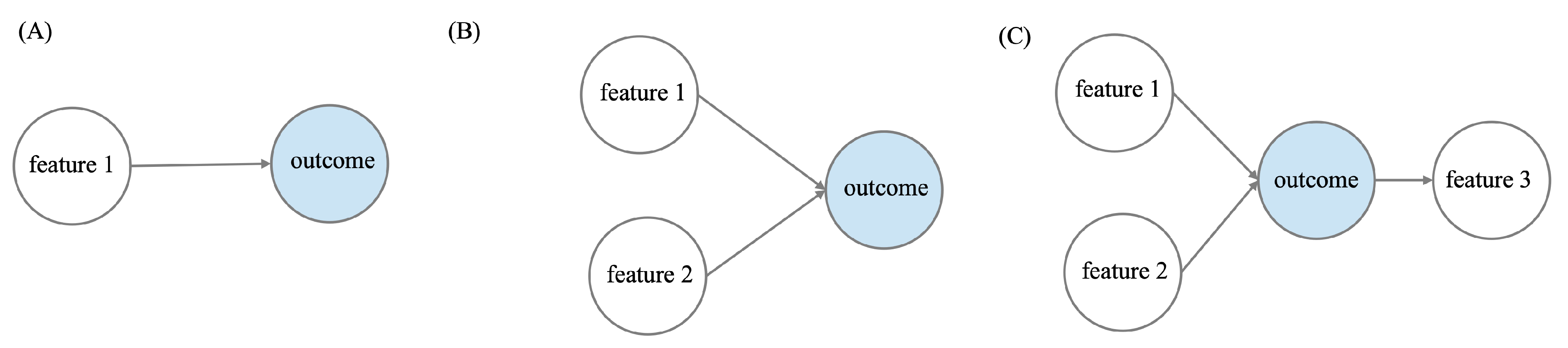
Figure 2. Comparison of AUC metric in training and validation folds

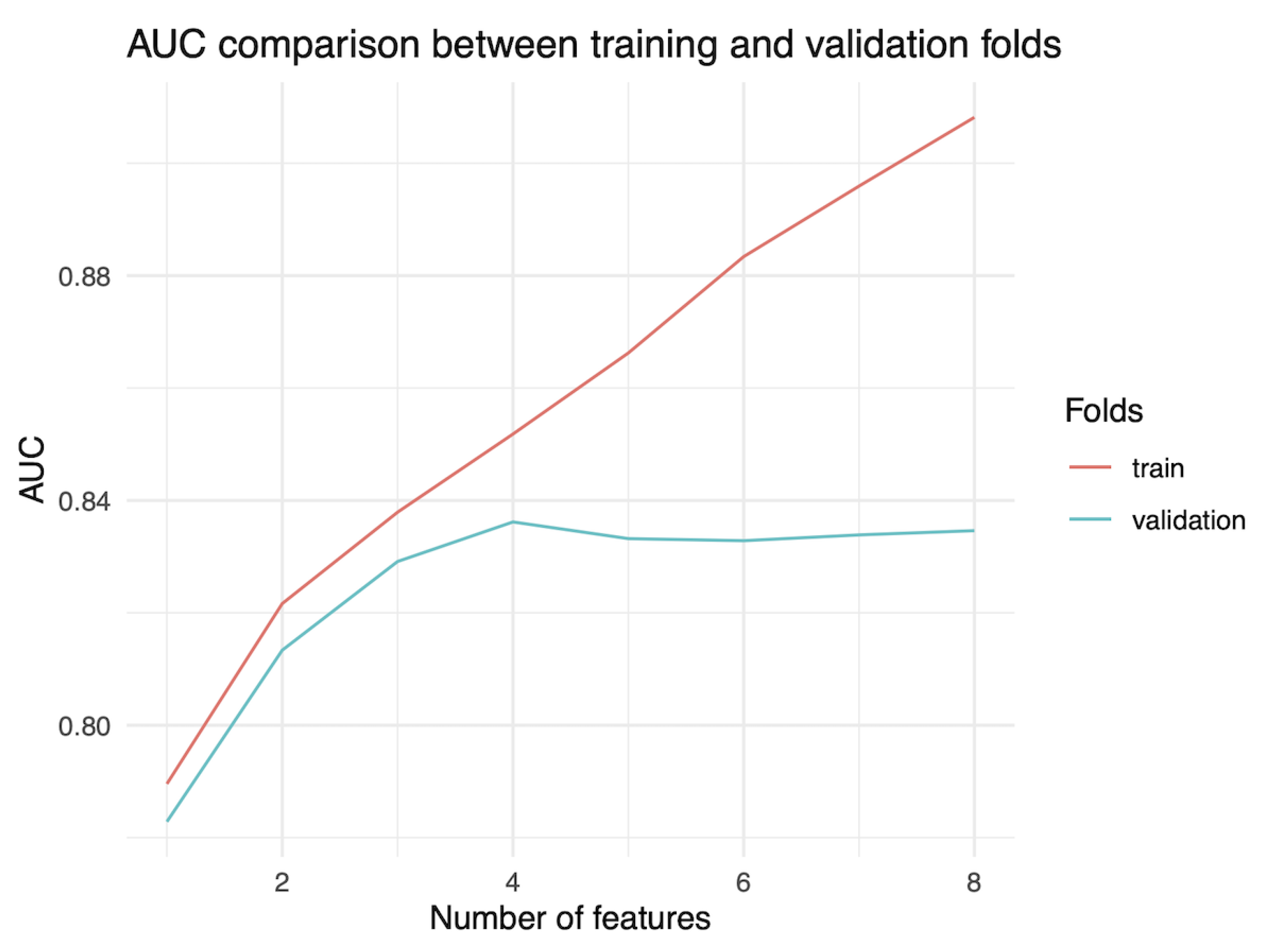
Figure 3. Optimal Bayesian network

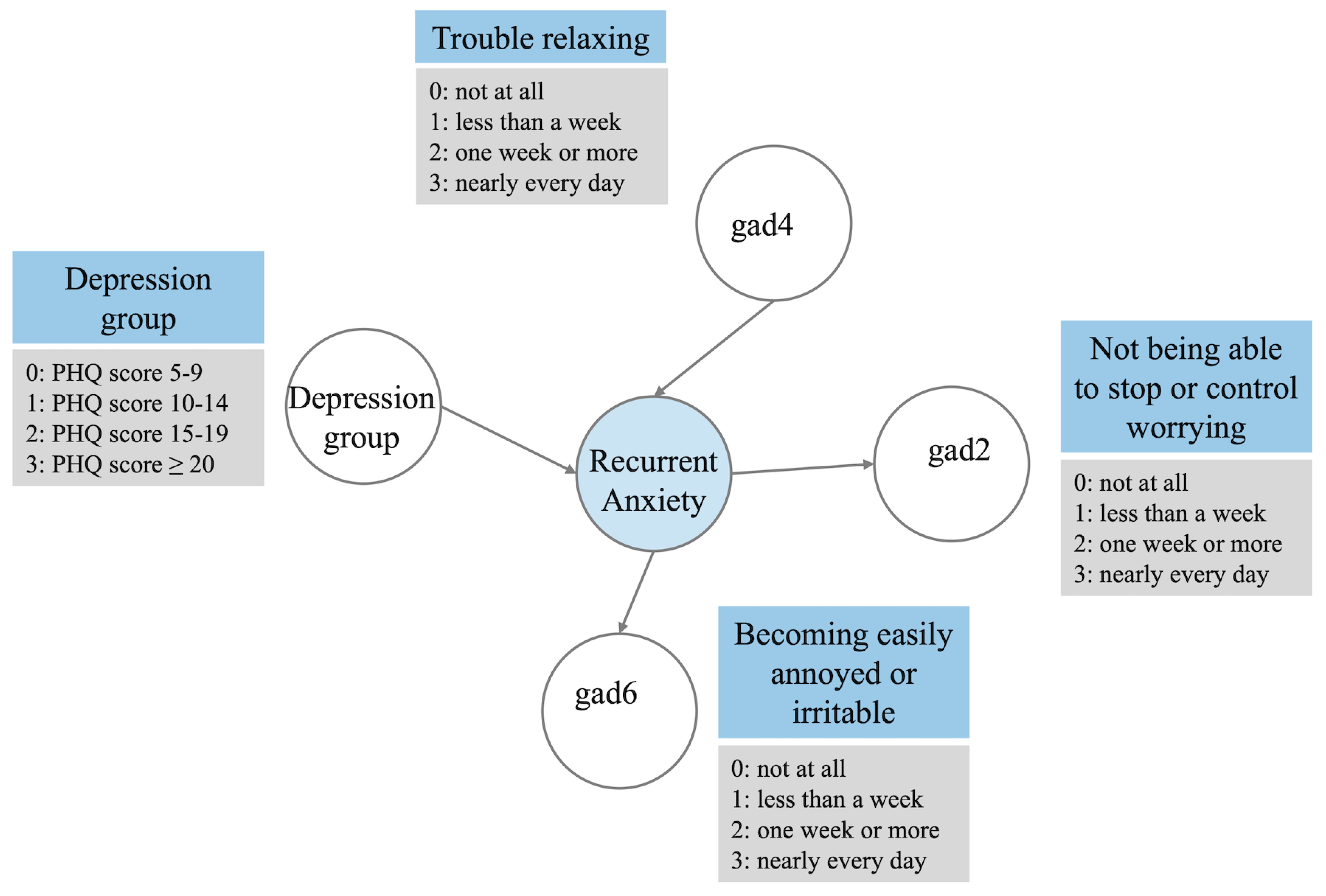
Table 1. Bootstrap output example

Index	From	To	Strength	Direction
1	Feature 1	Outcome	0.93	0.86
2	Feature 2	Outcome	0.84	0.74
3	Outcome	Feature 3	0.75	0.55
4	Feature 4	Outcome	0.41	0.66
5	Feature 5	outcome	0.21	0.77

Table 2. Results of the 1000 samples bootstrap

Index	From	To	Strength	Direction
1	Recurrent anxiety	gad6	0.33	0.58
2	Recurrent anxiety	gad2	0.27	0.54
3	Depression group	Recurrent anxiety	0.12	0.58
4	gad4	Recurrent anxiety	0.11	0.82
5	ucla3	Recurrent anxiety	0.11	0.55
6	gad1	Recurrent anxiety	0.06	0.67
7	Recurrent anxiety	ucla1	0.03	0.67
8	phq5	Recurrent anxiety	0.03	0.83
9	depression	Recurrent anxiety	0.01	1

Table 3. AUC metric summary of repeated cross-validation

Index	Mean AUC	Min AUC	Mean AUC	Max AUC	Std AUC
BN	train	validation	validation	validation	validation
1	0.790	0.648	0.783	0.913	0.051
2	0.822	0.648	0.813	0.928	0.056
3	0.838	0.648	0.829	0.959	0.057
4	0.852	0.648	0.836	0.959	0.056
5	0.866	0.648	0.833	0.959	0.054
6	0.883	0.648	0.833	0.959	0.053
7	0.896	0.648	0.834	0.959	0.052
8	0.908	0.648	0.835	0.964	0.051
9	0.918	0.648	0.835	0.964	0.050

Table 4. F1-score metric summary of repeated cross-validation

Index	Mean F1	Min F1	Mean F1	Max F1	Std F1
BN	train	validation	validation	validation	validation
1	0.766	0.633	0.766	0.903	0.045
2	0.756	0.538	0.745	0.903	0.052
3	0.771	0.538	0.759	0.918	0.055
4	0.784	0.538	0.765	0.918	0.053
5	0.793	0.538	0.758	0.918	0.055
6	0.807	0.538	0.757	0.918	0.053
7	0.818	0.538	0.759	0.918	0.053
8	0.835	0.538	0.759	0.918	0.052
9	0.835	0.538	0.760	0.918	0.052

Table 5. Comparison of AUC and F1-score on training, validation and test data

	Training	Repeated cross-validation	Test
AUC	0.889	0.836	0.821
F1-score	0.831	0.765	0.743

Table 6. Model performance comparison based on AUC metric

	Min¹	Mean²	Max³	SD⁴	Test⁵
Logistic regression	0.805	0.897	0.973	0.037	0.814
SGDClassifier	0.706	0.883	0.971	0.05	0.842
XGBoost	0.758	0.884	0.96	0.039	0.799
Bayesian network	0.648	0.836	0.959	0.056	0.821

¹Min: Minimum AUC value for 100 evaluations: repeated cross-validation for Bayesian Network, nested cross-validation for the remaining models. ²Mean: Mean AUC value for 100 evaluations: repeated cross-validation for Bayesian Network, nested cross-validation for the remaining models. ³Max: Maximum AUC value for 100 evaluations: repeated cross-validation for Bayesian Network, nested cross-validation for the remaining models. ⁴SD: Standard deviation of AUC values for 100 evaluations: repeated cross-validation for Bayesian Network, nested cross-validation for the remaining models. ⁵Test: AUC value on the test data.

Disclaimer/Publisher’s Note: The statements, opinions and data contained in all publications are solely those of the individual author(s) and contributor(s) and not of MDPI and/or the editor(s). MDPI and/or the editor(s) disclaim responsibility for any injury to people or property resulting from any ideas, methods, instructions or products referred to in the content.

© 2024 by the authors. Licensee MDPI, Basel, Switzerland. This article is an open access article distributed under the terms and conditions of the Creative Commons Attribution (CC BY) license (http://creativecommons.org/licenses/by/4.0/).

Copyright: This open access article is published under a Creative Commons CC BY 4.0 license, which permit the free download, distribution, and reuse, provided that the author and preprint are cited in any reuse.

MDPI Initiatives

Important Links

Choose an area of interest and we will send you notifications of new preprints at your preferred frequency.

Disclaimer