Submitted:
15 July 2024
Posted:
16 July 2024
You are already at the latest version
Abstract
Deep learning neural networks require an immense amount of computation, especially in the training phase of the network when networks with multiple layers of intermediate neurons need to be built. In this paper, we will focus on the PSO algorithm with the aim of significantly accelerating the DLNN training phase by taking advantage of the GPGPU architecture and the Apache Spark analytics engine for large-scale data processing tasks. PSO is a bio-inspired stochastic optimization method whose goal is to iteratively improve the solution to a (usually complex) problem by attempting to approximate a given objective. However, parallelizing an efficient PSO is not a straightforward process due to the complexity of the computations performed on the swarm of particles and the iterative execution of the algorithm until a solution close to the objective with minimal error is achieved. In the present work, two parallelizations of the PSO algorithm have been implemented , both designed for a distributed execution environment. The synchronous parallel PSO implementation ensures consistency at the cost of potential idle time due to global synchronization, while the asynchronous parallel PSO approach improves execution time by reducing the need for global synchronization, making it more suitable for large datasets and distributed environments such as Apache Spark. Both variants of PSO have been implemented to distribute the computational load supported by this algorithm –due to the costly fitness evaluation and updating of particle positions– across the different Spark cluster executor nodes to effectively achieve coarse-grained parallelism, resulting in a significant performance increase over current sequential variants of PSO.
Keywords:
Apache Spark
; Classification recall
; Deep Neural Networks
; GPU Parallelism
; Optimization research
; Particle Swarm Optimization (PSO)
; Predictive Accuracy
1. Introduction
The increasing use of applications with intelligence at the edge, not just in the cloud, requires the optimization of load balancing, workload placement and resource provisioning, especially when resource-intensive tasks need to be moved out of the cloud. This is because in DLNN with many intermediate layers of neurons and a lot of input data, the amount of computation to be performed is enormous and requires evaluating of the fitness of a very large number of particles. In recent articles [1,2,3] it has long been demonstrated that the training phase of neural networks can be accelerated by using different approaches [4,5,6,7,8,9,10].
In our proposal we have used the Apache Spark analytics engine, which supports RDD and the use of lambda functions and a functional programming style of Scala and Java languages and on a Java JVM. The basic idea that motivates our work is to go beyond existing studies on parallelizing the PSO algorithm to date [11,12,13,14,15,16], to create a new algorithm that achieves greater independence between the processes themselves, so that they can specialize in the parallel computation of functions of the algorithm, but without the need for synchronization points or collection of partial results between such processes.
PSO is one of many other algorithms known as metaheuristics, a class of optimization algorithms that are commonly used to find near-optimal solutions to complex optimization problems. Using PSO in an edge computing environment can make it feasible to train DLNN on edge devices rather than in centralized data centers or cloud environments. Edge devices are typically situated closer to the data source, such as IoT devices, smartphones, and embedded systems, and they often have limited computating resources compared to traditional centralized hosts. However, achieving an efficient PSO implementation is not straightforward due to the complexity of the computations that are inferred on the particle swarm and their own iterative execution until convergence to a solution close to the target with minimal error is achieved.
An example of multi-objective evolutionary multiheuristic approaches has been proposed in [17] to optimize the energy performance of buildings by balancing energy consumption and comfort levels. They implemented a PSO–based method with an improved update strategy to overcome the problem of local convergence. Another PSO-based solution was proposed in [11], which integrates an energy-efficient clustering approach to address the problem of limited sensor battery life. A butterfly-inspired algorithm was proposed in [18] to minimize the energy consumption of an office building in Seattle. And an ant colony optimization approach in [19] to estimate energy demand of Turkey. There are many other optimization algorithms commonly used in literature such as Artificial Bee Colony [20], Harmony Search [21], Firefly Algorithm [22], Cuckoo Search [22] or Gravitational Search Algorithm [23].
Several studies have investigated the application of PSO for solving forecasting problems. For example, [16] proposed a DLNN model with efficient feature fusion for predicting building power consumption. They integrated temperature data and applied an innovative feature fusion technique to improve the learning ability of the model. The study conducted extensive ablation studies to evaluate the performance of the proposed model. In [12], it was proposed a hybrid PSO and NN algorithm for building energy prediction and introduced two modifications to improve its performance. They compared their proposed model with simple ANN and SVN and demonstrated the effectiveness of their approach. PSO was used in combination with Adaptive Neuro Fuzzy Inference System (ANFIS) to determine industrial energy demand in Turkey, in [14]. The PSO algorithm was used to optimize the parameters of the ANFIS model. A common strategy for modifying PSO is to adjust its control parameters, as discussed by [13]. Another approach is to hybridize PSO with other metaheuristic algorithms such as Genetic Algorithms (GA) [24] and Differential Evolution (DE) [25] In addition, parallelization and multi-swarm techniques have been used to improve the performance of PSO, which has been applied to energy consumption prediction in various domains. For example, [15] proposed a multi-swarm PSO algorithm for static workflow scheduling in cloud fog environments. Their approach outperformed the classical PSO [26] and other approaches in terms of execution time and stability.
Thus, the motivation arises to realize the parallelization of the PSO algorithm according to two different parallelization schemes, which are discussed in Section 3. The first parallelization, DSPSO, follows a synchronous scheme, i.e., the best global position found by the particles is globally updated before executing the next iteration of the algorithm. DSPSO proved to be more efficient on medium sized datasets (<40000 data). The second implementation, called DAPSO, is an asynchronous parallel variant of the PSO algorithm that showed lower execution time for large datasets (> 170,000 data) that DSPSO and also presents better scalability and elasticity with respect to increasing in dataset size. Both variants, DSPSO and DAPSO, have been implemented for a distributed execution environment to distribute the particle fitness computation and particle position update, among the different execution nodes of an standalone Spark cluster, to effectively achieve coarse-grained parallelism, which has provided us with significant performance gains over current sequential variants of PSO.
In addition, a library was built in Scala that implements the parallelization of the learning process of multilayer feed-forward neural networks using both variants of the PSO algorithm, allowing us to perform the training of a neural network in a distributed manner using Spark. The neural networks were programmed as part of the case study to solve a regression problem and a classification problem. In this way, we can verify that the implemented networks work correctly. On the other hand, we compare the efficiency of the implemented DSPSO and DAPSO variants with their sequential variants, since a comparison with another learning algorithm is not reasonable.
In the current literature, it is common to see authors using machine learning models such as Artificial Neural Networks (ANN) [27], Support Vector Machines (SVM) [28] or Random Forests (RF) [29] to solve a variety of problems. However, these authors often limit their efforts to specific parameters and do not consider other important aspects of the modeling process, such as optimizing the model structure. This can lead to suboptimal performance and a lack of robustness in their models. In order to achieve optimal results, it is critical to consider not only the choice of model and its parameters but also to follow an optimization strategy. In the case of ANN, this may include selecting the optimal number of layers, nodes, activation functions as well as fine-tuning the connection weights. A well-optimized model structure can improve the accuracy and robustness of the model, and ultimately lead to better results [6]. While the time cost of developing optimization strategies is a common challenge faced by researchers, the use of a GPU parallel strategy can potentially help mitigate this problem. By implementing and using two variants of the PSO distributed synchronously and asynchronously, we intend to leverage the strengths of the PSO algorithm to train the DLNN to, for example, predict energy consumption more efficiently and solve complex classification problems with good accuracy.
The rest of the paper is organized as follows: Section 2 gives an overview of PSO algorithms, their common control structure, and the sources of complexity of their parallelization on distributed computing platforms. Section 3 presents the two PSO parallelizations proposed in this work and the pseudocodes of both variants, along with general details about them, according to the conditions imposed by many-core GPU architectures, for use in training DLNN and obtaining the measurements and plots shown to test their efficiency and scalability. Section 4 explains the results of the experiments and discusses the two case studies proposed to evaluate a Spark-based implementation of both PSO variants. Finally, the last section summarizes the conclusions and future work.
2. Particle Swarm Optimization
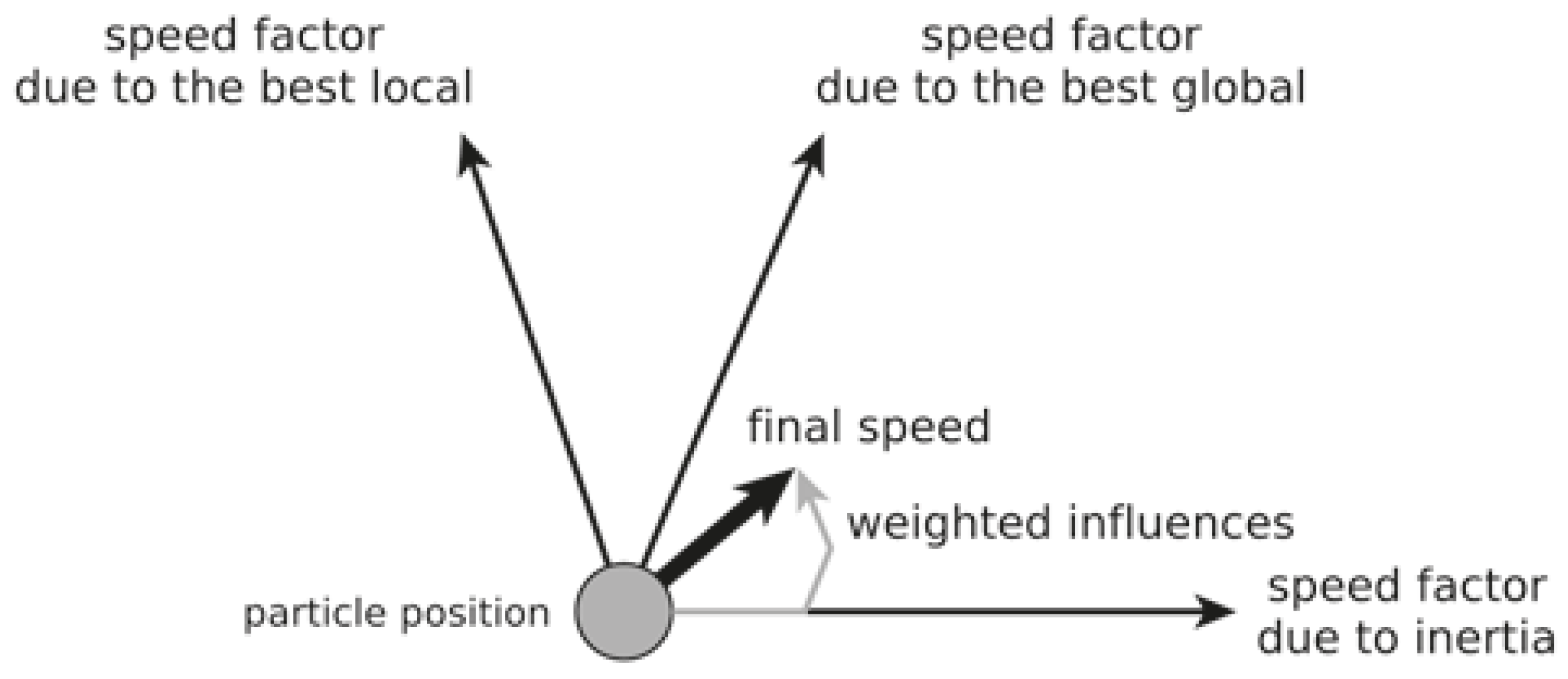
Particle Swarm Optimization (PSO) is a bio-inspired stochastic optimization algorithm. Invented by Eberthart and Kennedy in 1995 [26], PSO is an algorithm whose goal is to improve a randomly generated solution iteratively with respect to a given objective. The algorithm focuses on a population of entities called particles. A particle is represented as a point in an N-dimensional Cartesian coordinate system. Particles are abstractions of entities that are at a position and move with a velocity. Initially these particles are randomly assigned a position and velocity. In addition each particle keeps track of its personal best position and global best position , which is reached by other particles up to that time and detected by the current particle. Thus, the positions and velocities of each particle are updated at each time t as follows,
and are non-negative constants called learning factors and and are two random numbers with uniform distribution in the interval . Also note the inertia constant which allows balancing the local and global search and which is a value in the interval . In addition, the maximum velocity is restricted to the values of .
In addition each particle keeps a record of the personal best position and global best position achieved by other particles up to that time and detected by the current particle. The best position is measured using the fitness function, which is what we seek to optimize, therefore, the term best refers here to the minimum or maximum value found during the evaluation of the particle position with the fitness function defined in the algorithm. The fitness is a type of objective function used to calculate how close a given solution is to achieving the objectives initially established in the algorithm.
Figure 1.
Graphical representation of a PSO algorithm’s particle with its attributes.
PSO works through iterations, during which all particles are evaluated for their fitness in terms of local and global best position. The way to detect the best position and the fitness reached by the other particles will depend on whether there is common memory among them and then it will be done by reading a global variable. In case of distributed systems, there is no such shared memory, and a message passing protocol has to be implemented that, in a first approximation, ensures the coherency of the value of the global best position for all the particles. At the end of each iteration, all particle velocities and positions must be updated, which is a drawback for the asynchronous parallel implementation of such updates.
The solution proposed here for the implementation of the distributed parallel PSO algorithm consists of the design and implementation of two variants of the distributed PSO, which we have called distributed synchronous (DSPSO) and distributed asynchronous (DAPSO).
The DSPSO variant makes use of the most common form of implementation based on serial iterations. First the fitness of each particle is evaluated with the position of the particle as input, then the best local position of each particle is evaluated and then the best global position among all particles is determined. Finally, the position and velocity of each particle is updated based on the best global position.
The second variant, DAPSO, changes from the previous variant in the information available when updating the particles, in such a way that they are updated as soon as their fitness is evaluated and, therefore, the update of the position and velocity of the individual particles does not have to wait for the evaluation of the fitness of all the others, as occurs in the DSPSO variant, thus avoiding a synchronization of the type barrier or multiple rendez-vous between processes and that the particles suffer undesired waits due to the fact that each one of these has to know the data of the others before proceeding to its update. In this way the desired asynchronicity of the calculations between particles is achieved, which move to the next position with the information available at that moment, so that several values of the global best position could coexist during the execution, which in a later stage of the algorithm will have to converge in only 1 global value. The validity of the final result of the global best position is not affected because the communications that will be established between the processes in charge of updating the position and velocity of each particle ensure the coherence of the global position and velocity that will be finally communicated to each particle will be achieved.
2.1. Complexity of the PSO and Approaches for Its Parallelization in a Cluster
The classical PSO algorithm works on the basis of iterations, during which particles are evaluated in terms of their fitness and their personal and global best positions. At the end of each iteration, the velocities and positions of all particles have to be updated, which is a drawback for the asynchronous parallel implementation of such an update.
The use of PSO for solving prediction and classification problems has advantages and disadvantages,
- As a metaheuristic algorithm, no specific knowledge of the problem to be solved is required
- As an evolutionary algorithm, it is easy to adapt to parallel computing structures.
- Being able to work with different solutions, it has a higher tolerance to local maxima or minima.
- The main disadvantage is that the PSO algorithm needs a large amount of time to reach a good solution in problems of high complexity, i.e., with a large number of particles or with many dimensions, because many evaluations of the fitness function are required.
The use of parallelization of the PSO algorithm to train neural networks represents a cutting-edge strategy with multiple applications and outstanding benefits in the field of machine learning and artificial intelligence. Among the benefits of parallelizing the PSO algorithm [30], we can mention: efficiency improvement, faster scanning of solutions, scalability, increased accuracy and reduction of development time.
The first variant considered here is the Distributed Synchronous PSO (DSPSO), which uses the most common form of iteration. First, the fitness of each particle is evaluated using the particle’s position as input. Then the best personal position of each particle is evaluated to determine the best global position among all particles, and finally the position and velocity of each particle are updated based on the best global position.
The second variant studied and fully implemented is the so-called distributed asynchronous PSO (DAPSO), which differs from the previous one in the information available when updating the position and velocity of the particles, so that they are updated as soon as their fitness is evaluated and, therefore, the update of the position and velocity of each particle is not necessarily consistent in all the nodes of the cluster during the computation of this variant of the PSO. The distributed nature of this computation will make its execution faster than that of the DSPSO, without affecting the validity of the final result, since the communication that will be established between the processes in charge of updating the position and velocity of each particle will ensure that, in the end, the consistency of the global position and velocity that will be finally detected by each of the particles in the algorithm will be achieved.
2.2. Background Information Based on Recent Research on the Parallelization of the PSO
The use of parallelization of the PSO algorithm to train neural networks represents an efficient and scalable approach with several practical applications and notable advantages, such as the ability to process DLNN with many layers of intermediate neurons in a much shorter time frame than with traditional implementations that do not take advantage of the massive parallelism currently provided by multicomputers or, in our study, by GPGPU. This makes it an extremely valuable tool in the field of machine learning and optimization.
There are currently many implementations of PSO using the CUDA/GPU environment. One of them, called PSO-GPU [1], presents a generic and customizable implementation of a PSO algorithm on top of the CUDA architecture, taking advantage of the thousands of threads running on the GPU to reduce execution time and increase performance through parallel processing. One strategy currently used to improve PSO algorithm implementations is to adjust its control parameters, thus gaining efficiency without losing precision in determining the objective, as described in [13]. In [2], an asynchronous parallel PSO algorithm is presented that significantly improves parallel efficiency. Parallel PSO algorithms have mainly been implemented synchronously, where the fitness functions, positions and velocities of all particles are evaluated in one iteration before the next iteration starts. The latter approaches usually result in a small speedup of the parallel computation over the sequential variant in cases where a heterogeneous parallel environment is used and/or where the execution time depends on the element of the algorithm being computed. Therefore [2] was the first work to explore an asynchronous parallel implementation of the PSO algorithm and significantly improved the parallel efficiency of PSO implementations at the time of its publication. This approach had similar goals to those of our study, which focuses on the speedup of the asynchronous PSO algorithm over the synchronous one.
A hybrid mechanism of Spark-based particle swarm optimization (PSO) and differential evolution (DE) algorithms (SparkPSODE) is proposed in [31]. SparkPSODE is a parallel algorithm that uses RDD and island models. The island model is used to divide the global population into several subpopulations, which are used to reduce the computational time corresponding to the RDD partitions. SparkPSODE is applied to a set of global large-scale optimization benchmark problems and is shown to achieve better performance (speedup, scalability, robustness) of the sought optimization according to the experimental results obtained with respect to other algorithms.

Table 1.
Selected approaches for improvement in PSO algorithm implementation to date
| Main strategy | References | Years |
|---|---|---|
| Accelerating PSO in CUDA/GPU | [1,2] | 2011, 2005 |
| Adjustment of control parameters | [13] | 2002 |
| Hybrid mechanisms with PSO | [24,25,31] | 2019, 2015, 2020 |
| Big Data & PSO | [32] | 2020 |
There is currently work using Spark to parallelize the genetic algorithm and tackle the problem with very good results; in [25], the GPU is used to parallelize an evolutionary training algorithm. One of the ways to address the problem of climate change and its consequences is to study the energy consumption of the buildings around us. Studying energy consumption can provide us with relevant information to make better decisions and thus reduce costs and pollution. However, ANN training models based on evolutionary methods generally have a high computational cost in terms of time. This paper takes advantage of the high-performance computing capabilities of GPUs to parallelize the PSO evolutionary algorithm to train the ANN.
Another area of intense research is the parallel implementation of PSO for big data datasets. Traditional methods cannot meet the requirements of Big Data environments for prediction, so a hybrid distributed computing framework is applied in Apache Spark [32] for wind speed prediction using a distributed computing strategy, the framework can divide the speed data into RDD groups and operate them in parallel.
The main problem with many of these solutions lies in the fact that they are all limited to parallelizing the repetitive process of the algorithm, based on a population size of the dataset, necessary to be able to accurately compute the population fitness function, but without generally considering further advances in terms of parallel structure of the subtasks of the algorithm, which is one of the main objectives of our study.
3. PSO Parallelization Based on Apache Spark and RDD Applied to Training Neural Networks
To carry out this study, we need to perform an efficient parallelization of the PSO algorithm according to the conditions imposed by GPGPU architectures of many cores, to use it in the training of a neural network and to obtain the measurements of the following section. We use the MSE for continuous variables to compute fitness, which we will use to solve regression problems; and the measures of binary cross-entropy and precision for categorical variables in classification. Both variants of the distributed PSO implemented in this study were applied to the training of neural networks to solve two problems: (a) a regression problem to predict the consumption of the institution’s buildings in kilowatt hours, (b) classification based on the use of a Kaggle dataset to predict whether a set of people are smokers or not, using a binary objective.
3.1. Distributed Synchronous PSO
The distributed synchronous PSO adopts the master/worker paradigm, where the master maintains the state of the entire swarm and sends particles to each worker node for evaluation. The master also manages the synchronization required to control specific iterations of the DSPSO, and updates global data relevant to the algorithm through variables of type Broadcast, which are a type of read-only shared variable, e.g., from the Scala programming language, that are cached and available on all nodes in a Spark cluster to be accessed or used by tasks. The tasks performed by the master and worker nodes in this variant are given by the Algorithm 1 expressed in pseudocode.
| Algorithm 1 DSPSO pseudocode |
|
The function fitnessEval (f) is executed on the worker nodes and is responsible for receiving a particle, calculating the fitness of the current particle position using the variable broadVar of the Scala Broadcast type mentioned above, and then updating the personal best position of the particle and finally returning it. The pseudocode uses closure anonymous function type, which includes its execution environment.
3.1.1. Each Worker Node Should Perform the Following Steps:
- wait for a particle to be received from the master node,
- compute the fitness function f and update the personal best position ,
- return the evaluated particle to the master node,
- return to step 1 if the master node has not finished yet.
3.1.2. The Master Node Process Includes the Following Steps:
- initialize particle parameters, positions and velocities;
- assign the current iteration and initialize the state of the swarm and the received particles;
- start the current iteration by distributing all particles to the free executors;
- wait for the results of all evaluated particles (with calculated fitness function) and the personal best position for this iteration, which means for sync;
- computing the global best position for each incoming particle until there are no more particles left;
- updating the velocity vector and the position vector of each particle based on the personal best position and the global best position found by all particles:
- going back to step 3 if the last iteration has not been reached;
- return the global best position .
3.2. Distributed Asynchronous PSO
DAPSO differs from DSPSO in synchronization becasuse there are no iterations linking all particles. In DAPSO, each particle is evaluated and moves independently of the other particles. This further increases its independence.
We will now discuss the implemented DAPSO variant, which is distributed and asynchronous, and uses Spark RDDs to parallelize the updating of particle positions and velocities. Using Spark and its low granularity transformations, the swarm is divided into several sub-swarms that are evaluated in parallel. The particles are updated according to the current state of the entire swarm, i.e., both the position and velocity of each particle are modified as soon as the fitness function is evaluated, taking into account the best global position found so far. This creates complete independence between the particles, which move to their next position with the information available to them at the time of each particle’s evaluation.
The DAPSO distributed algorithm follows the master-worker paradigm: a master node is responsible for coordinating the rest, the worker nodes, which are responsible for performing the computations sent by the master. Each particle in the swarm moves and evaluates the fitness function autonomously.
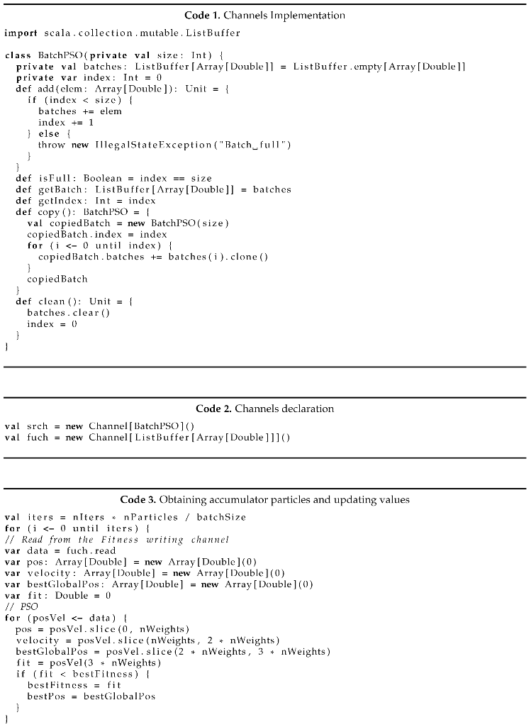
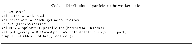
For efficiency, the algorithm uses an abstraction called SuperRDD, which consists of a set of particles that are interdependent and run in the cluster as a single subswarm. That is, instead of sending each particle to the cluster independently, they are grouped into subswarms of variable size between 1 and S, where S is the number of particles. The larger the size of the subswarm, the lower the degree of asynchronicity of the algorithm, since more particles are dependent on each other. However, this change improves the efficiency of the algorithm by removing some of the computational overhead of communication between the nodes, which partially sacrifices asynchronicity as the master node pauses the global computation while waiting for the partial results of the subswarm. In the context of Spark, the SuperRDD consists of the grouping of multiple individual RDD particles that are then evaluated.In the context of Spark, the SuperRDD is the grouping of multiple individual RDD particles that are then evaluated by the cluster. In this way, and as the number of particles in the RDD increases, fewer Spark jobs need to be scheduled, reducing the communication overhead, at the cost of the particles having to wait for the rest of the RDD to be evaluated by the node.
As for the implementation in Scala and Spark, two concepts are key to proper operation: an accumulator that receives the evaluated particle data (or SuperRDDs) from the worker nodes and a way to distribute these particles to the worker nodes. The best global position update is performed by the broadVar, as in the DSPSO algorithm. The accumulator implementation (see Appendix A) consists of a communication channel capable of storing lists of numbers. We will call this the accumulator channel. The worker nodes, when evaluating the particles, send to this channel a list containing the position of the particle, its velocity, and the processed value of its fitness. The master node then reads the elements of this channel to update the particle values. In the pseudocode 2, represents the channel to send particles in one batch to the worker nodes and is the fitness update channel to receive the updated values of these particles.
| Algorithm 2 DAPSO pseudocode |
|
3.2.1. The Master Node Process Consists of the Following Steps:
- initializing the particle parameters, positions and velocities,
- initializing the state of the swarm, as well as that of a particle queue to send to the worker nodes,
- loading the initial particles into the queue,
- distributing the particles from the queue to the available executors,
- waiting for the results of all evaluated particles (with calculated fitness function) of the subswarm and the personal best position for this iteration,
- updating the velocity vector and position vector of each particle based on the personal best position and the global best position found by all the particles,
- placing the particle back in the queue and returning to step 4 if the stop condition is not satisfied,
- return the best global position .
3.2.2. The Process of Worker Nodes
Same as in the synchronous variant.
3.3. Apache Spark Implementation
This work was not programmed directly in CUDA, but used an open-source data processing framework with a processor cluster architecture that allows for massively parallel and distributed computations. This is the main feature of the analytics engine known as Apache Spark [33], designed for efficient processing and analysis of large amounts of data, with the ability to achieve scalability and quality of service when implementing ML models. Spark is implemented in the Scala programming language, which is why it has been chosen as the primary programming language in this study.
Based on RDDs, resilient distributed datasets, described by Matei Zaharia in [34], Spark is the most widely used tool for performing scalable computational tasks and data science. RDDs are fault-tolerant parallel structures that allow intermediate results to be persisted in memory and manipulated by a set of operators. They are particularly useful for applications where intermediate computations are reused across multiple computations, such as most iterative machine learning algorithms: logistic regression, K-means, ⋯ Formally, an RDD is a partitioned collection of read-only data sets that can be created from deterministic operations on data in stable storage or from other RDDs. We will call these operations transformations to distinguish them from other operations. Examples of these transformations include mapping, filtering and joining. The main goal of RDDs is to define a programmatic interface that is able to provide fault tolerance in an efficient way. On the other hand, distributed shared memory architectures provided an interface based on fine-grained updates of mutable states such as cells in a table. The only way to provide fault tolerance in the latter is to replicate data to other machines or to log updates on nodes, which unlike Spark RDDs, turns out to be quite inefficient.
There are three important features associated with an RDD: dependencies, partitions (with some locality information) and transformations (computational functions). First, you need a list of dependencies, which tell Spark how to construct an RDD from its inputs. When results need to be replicated, Spark can rebuild an RDD from these dependencies and replicate operations on it. This feature gives RDDs resiliency. Second, partitioning gives Spark the ability to divide the work of parallelizing computations into partitions by mapping them to Spark cluster executors. Third, transformations apply to data frames as follows: Partition Iterator[T]. All three are fundamental to the simple RDD programming model on which all top-level application programming functionality is based, which approximates a functional programming paradigm.
In the Spark environment, data are fragmented into partitions, which are the elementary unit of data that can be processed autonomously. RDDs are segmented into these partitions and distributed across the cluster. The number of partitions is generally adjustable and depends on factors such as data volume and availability of resources in the system. Associated with each RDD are partitions that provide Spark with the ability to divide the work of parallelizing the computation among executors in the Spark cluster. In some cases, for example, when reading from HDFS, Spark uses locality information to send work to executors close to the data. In this way, less data are transmitted over the network (Figure 2) and greater efficiency is achieved than using the map/reduce distributed computing and Hadoop .
In the main loop of a neural network implemented for solving prediction problems, we can find three distinct parts, the computation of the fitness function, the update of local and global data values, and finally the output of results that can change over time and have time constraints. To achieve the required efficiency of the ANN training implementation, Spark RDDs have been used for both DSPSO and DAPSO implementations, where each row contains a particle with the information of its position, velocity, personal best position and personal best fitness. With this information the particle’s fitness can be computed and its personal best position and fitness can be updated, computations that are performed in parallel for each particle in the RDD using Spark. Instead of setting this data along with each task on the cluster executors, Spark distributes the broadcast variables to the machines using efficient broadcast algorithms to achieve lower communication costs in massively parallel applications.
4. Case Study and Applications
We propose two cases for evaluating a Spark-based implementation that can run on both CPUs and GPUs to take full advantage of the performance capabilities that the DSPSO and DAPSO variants of the PSO algorithm implementation can offer us, as follows
- efficiency improvement: parallelization leverages the computing power of multiple resources, such as graphics processing units (CPUs or GPUs) or central processing units (CPUs), thus speeding up the training process,
- faster scanning: parallelization techniques for the PSO algorithm allow multiple solutions to be evaluated simultaneously, speeding up the search for optimal solutions in a large parameter space,
- scalability: It can handle problems of varying size and complexity, from small tasks to large challenges with massive data sets,
- increased accuracy: by enabling faster and more efficient training, parallelization of the PSO algorithm can improve the quality of the neural network models that are designed, resulting in better performance in prediction and classification tasks,
- reduction of development time:parallelization reduces development time by speeding up the training process, leading to faster development of machine learning models.
Predicting energy consumption (EC) across a range of buildings is a formidable challenge. This explains why companies and governments around the world are focusing their efforts in this area. One of the most critical areas to address this problem is the prediction of energy consumption (EC) at the local level, for example, in buildings associated with an organization or institution. This allows us to anticipate future events and, as a result, make more informed decisions about energy savings. In this context, the analysis of energy consumption recorded by sensors at the individual level, in specific areas or buildings, has the potential to reduce energy costs and mitigate the environmental impact derived from energy production.
In addition to its application to regression problems, the PSO algorithm can also be used to train neural networks focused on solving classification problems. To this end, we propose here a second case study, to develop which we have taken a dataset from the Kaggle platform corresponding to the challenge Binary Prediction of Smoker Status using Bio-Signals challenge. The Kaggle website can be found here: https://www.kaggle.com/competitions/playground-series-s3e24.
4.1. A Regression Problem: Prediction of the Electrical Consumption of Institution Buildings
In order to achieve the performance required for the application to make useful predictions about energy consumption, we propose here two Spark-based model implementations for useful EC predictions for a given time horizon, such as the hourly power consumption during the month and presented here, can be run on both CPUs and GPUs to take full advantage of the performance capabilities that such an implementation can offer us. Several studies have provided solutions to the problem of predicting EC in buildings using EAs and ANN. However, the main drawback of these methods is that they have an unreliable response time. So far, some approaches have been proposed to solve this problem [35]. As a result, there is still a lot of work to be done in this line of research, while interesting implementations of GPU-based EAs have been proposed in [1], where different data structures, configurations, data sizes and complexities have been studied to solve the problem.
The two variants DSPSO and DAPSO implemented in Scala/Spark in this study have been used here to solve a 24-hour EC prediction problem in buildings as one of the fundamental objectives of this work. To test the performance we have used the PSO algorithm as baseline and the Spark tool to train a perceptron–type neural network to make predictions about the EC of a set of buildings (Figure 3 and Figure 4) at the University of Granada, UGr (Spain). The performance of both algorithm implementations has been tested by measuring the execution time required to execute each of them. For this, we have used an abstraction related to each benchmark performed, according to which we always use a monotonic clock in our measurements, i.e., the time always goes forward and is not affected by hardware issues, such as time skew.
4.2. Performance Evaluation of a Regression Problem Implementation
To test the performance, we have used the implemented variants of the PSO algorithm and Spark primitives to train a perceptron neural network with the parameters given in Table 2, which correspond to the attributes in the rows of the dataset provided by the institution, such as the day, hour, and minute of the measurement, as well as the power scheduled for that day. We have evaluated the realized implementation of the DSPSO algorithm with synchronous individual update of particle velocity/position and that of the DAPSO algorithm with asynchronous distributed update of the same parameters. Moreover, to check the performance of each algorithm, only one of the first two constant parameters in Table 2 was increased at a time, while the other remained unchanged in each test. In this way were able to analyze how each algorithm reacts to an increase in the complexity of one parameter: particles, iterations , under certain conditions, individually. Figure 5(a) shows that, for a small number of particles (100,200), the distributed algorithms (DSPSO and DAPSO) perform slightly better than the traditional sequential PSO algorithm, as the overhead introduced by Spark affects the overall measured performance. However, when the number of particles increases to (500, 100), the distributed algorithms DAPSO and DSPSO are significantly faster, achieving on average 4 times and 2 times more speedup, respectively, than the traditional PSO. Figure 5(b) shows a similar behavior to the previous graph as the number of iterations is increased. The performance of DAPSO is observed to be similar to DSPSO for (500, 1000) iterations. This is because the number of Spark-jobs generated increases mainly with the number of iterations. Therefore, for a high number of iterations, the number of jobs created is similar for both algorithms. This differs from the observation in Figure 5(a) when the number of iterations is kept constant and the number of particles is increased. Therefore, both algorithms perform well regardless of the number of iterations or particles.
The performance of the distributed PSO algorithms is enhanced by using multiple executors for parallel fitness evaluation of particles on the Spark cluster. Of course, this performance is more visible on complex optimization problems where the overhead caused by Spark is negligible compared to the traditional PSO implementations. Figure 6 show the results relative to the error (MSE) of the measures of both the DSPSO and DAPSO implementations. The network was trained on 80% of the data (training set) and the remaining 20% was used to measure the errors (test set). In Figure 6, the errors obtained by both algorithms with 100 iterations (a) are much larger when using 12000 samples. This is due to the excessive task creation when there are not enough samples, resulting in a less representative search space. As a result, the particles may have difficulty converging to an optimal solution.
On the other hand, we observe that the error variability increases with the number of particles in the scan when using 12000 data. This is due to the updating made to the best position and fitness computed by the particles. However, as the number of particles increases, the errors converge to the same values as the asynchronous algorithm (DAPSO). This suggests that the reliability of both implemented variants depends mainly on the quality of the training data set. The DAPSO variant is generally more accurate, even with fewer samples. Finally, both graphs in the figure Figure 6(b) show that for more than 30240 samples, DAPSO produces the lowest error for higher values of the number of particles and iterations.
4.3. A Classification Problem: Binary Prediction of Smoker Status Using Bio-Signals
The PSO algorithm can be used to train neural networks focused on solving classification problems. Therefore, a dataset was selected from the Kaggle platform, corresponding to a competition where the objective is to predict the binary variable smoking using a set of biological characteristics such as the presence of caries or the levels of haemoglobin or triglycerides. The metrics to be used were accuracy, precision, recall and f1-score.
4.3.1. Statistical Study of Covariates
A statistical study of the covariates on the dataset was carried out using Python libraries, specifically the function from the scipy library to perform the chi-squared test (Table 3) and the statsmodels library to calculate the odds ratio and the relative risk. As most of the characteristics we have in the dataset are continuous, we have converted them to categorical variables, creating four categories for each continuous variable,
- Low: Those between the 0th percentile and the 25th percentile are classified here
- Medium low: Those between the 25th percentile and the 50th percentile are classified here
- Medium high: Those between the 50th percentile and the 75th percentile are classified here
- High: Those between the 75th percentile and the 100th percentile are classified here
In this case we will set a standard confidence level of 95%, i.e. a significance level of . Since the p-value is very close to 0 and much smaller than , we reject the null hypothesis that the variables are independent in all cases.
4.3.2. Odds Ratio Calculation
The odds ratio (OR) is used to quantify the association between two events. It compares the odds of the event occurring in one group with the odds of the event occurring in the other group. It is given by the equation
The odds ratio should be interpreted according to three ranges of values: OR ==1, there is no association between exposure and outcome; OR , indicates a positive association between exposure and outcome; OR , indicates a negative association between exposure and outcome.
The main results of Table 4 with odds ratio values are as follows: (1) Those with higher sugar and relaxation indices are more likely to smoke than those with low indices. (2) There is an association between smoking and higher body weight.(3) We see a significant increase in triglycerides (a type of blood fat) and haemoglobin and a large decrease in HDL. (4) We also see, although to a much lesser extent a decrease in LDL and an increase in serum creatinine which is a waste product present in the blood.(5) There is also a significant increase in alanine aminotransferase (ALT) which is an enzyme found mainly in the liver, the excess of which in the bloodstream can indicate damage to liver cells.
4.3.3. Relative Risk Calculation
The risk ratio (RR) is a statistical measure used to assess the relationship between the probability of a particular outcome in a group exposed to an event compared with a group not exposed. It is given by the equation
The results of the RR calculation are interpreted in the same way as the OR calculation. RR==1, there is no association between exposure and outcome. RR , suggests a positive association, i.e., exposure is associated with an increased risk of the outcome. RR , suggests a negative association between exposure and outcome.
The main results of Table 5 with RR values confirm those of Table 4 and are as follows: (1) There is again an association between smoking and higher body weight. (2) There is also an increase in blood glucose, although less steep than that seen in the odds ratio calculation. (3) As in the previous table, there is a significant increase in triglycerides (a type of blood fat) and haemoglobin and a large decrease in HDL. (4) There is also an increase in serum creatinine. (5) There is also a significant increase in alanine aminotransferase (ALT) and a large increase in guanosine triphosphate (GTP).
4.4. Evaluation of Classification Accuracy Based on Neural Networks Trained with the PSO
We carried out a validation process. We compared all the accuracy assessment points with the ground truth values. The calculated parameters are the next ones,
- -
- Precision: The precision is the probability value that a detected class element is valid. It is given by the equation
- -
- Recall: The recall is the probability value that a detected class element is detected in the ground truth. It is given by the equation
- -
- F1 score: This is a metric usually calculated to evaluate the performance of a binary classification model. It is given by the equationThe results obtained when contrasted with the interpretation of the ROC and Precision/Recall plots (Figure 7), indicate that the binary classification model we have obtained has a balanced performance. The obtained precision of 77% on average indicates that this percentage of positive predictions is correct and that the obtained classification has been performed reliably by the implemented PSO variants. The obtained recall implies that the model also correctly identifies 77% of all positive cases in the ground truth. F1–score calculated for 100 particles and 100 iterations: 0.7697050147492625, confirms that both measures of precision and recall are consistent with the results obtained, showing a balance between them and that the results have also been obtained with performance.
4.5. Assessment of Implementation Performance
The model appears to be robust and thus quite acceptable, as shown in the summary of one selected run of Table 7, with similar performance measured for the DSPSO and DAPSO variants, along with the near 0.77 accuracy (Table 6) discussed above, again indicating good predictive performance of both algorithms.
Table 7 contains information extracted from the Apache Spark Web UI (Web UI), which is a web-based graphical interface that provides detailed information about the status and performance of running Spark applications. In particular, it shows information about the executors in the cluster, including resource usage, especially memory blocks used by the entire computation, and the activity of Spark jobs or tasks. From the point of view of the distributed PSO algorithms implemented in this study, each job contains a set of particles whose fitness function is evaluated by the executor nodes. So, as the Table 7 shows, we have achieved concurrent execution of multiple jobs in the Spark cluster, where each job means parallel execution of multiple tasks. With the DAPSO implementation the master node collects asynchronously from the cluster the results of the execution of each task, updates the global variables, and returns the particle to the task, thus reusing the tasks and trying to achieve a better load balancing between them. In this way, DAPSO manages to significantly reduce the number of tasks for the fitness evaluation of each particle in the cluster. It can be observed in the table that only up to 5 simultaneously active tasks are necessary. We can say that DAPSO is much more a Spark-jobs “recycler” than DSPSO and therefore the memory usage is only 135 KiB versus the 25MiB needed by DSPSO to do the same job. We can therefore conclude that the DAPSO variant is more suitable for execution on resource constrained nodes in an edge architecture.
5. Conclusions
The two distributed implementations of the PSO algorithm presented serve to demonstrate the feasibility of their use in deep neural network training in a distributed-edge setting. The asynchronous DAPSO implementation improves the synchronous DSPSO one in terms of performance and accuracy, performing the tasks of fitness evaluation and particle update in a fully parallel and independent way by the workers of an Apache Spark cluster and yields really satisfactory results in terms of performance and scalability. While it has been noted that in problems with few samples, the problem size may be insufficient for DAPSO to achieve optimal performance, however, the MSE obtained with both variants are similar with a considerable amount of data and DAPSO is notoriously superior in terms of performance versus the synchronous DSPSO implementation, improving times in both the regression problem with 175104 samples and the classification problem presented here. In the latter one, due to the volume of the dataset with 127405 samples in the training set and 69 features used for classification, a huge improvement in execution times is achieved.
Regarding the implementation performed with an Apache Spark cluster, a higher performance has been observed with the DAPSO variant than with the implementation of the DSPSO variant. Although the programs developed with Spark can be executed on different distributed platforms, in this work the results shown refer only to the execution on a departmental GPU cluster. Therefore, as future work we want to design the presented algorithms for different platforms, such as Kubernetes or Databricks.
Funding
This research was funded by the Spanish Science Ministry (Ministerio de Ciencia e Innovación) grant PID2020-112495RB-C21.
Data Availability Statement
The code with the implementation of the trained neural network has been used to predict the energy consumption of a set of buildings in the University of Granada (Spain). The Scala/Spark code and the dataset used in this study are available at https://github.com/mcapeltu/PSO_Spark_Scala.git.
Abbreviations
The following abbreviations are used in this manuscript:
| ANN | Artificial Neural Network |
| DAPSO | Distributed Asynchronous PSO |
| DLNN | Deep Learning Neural Networks |
| DSPSO | Distributed Synchronous PSO |
| EA | Evolutionary Algorithms |
| EC | Energy consumption |
| GPGPU | General-purpose computing on Graphics Processing Units |
| MSE | Mean Squared Error |
| NN | Neural Network |
| PSO | Particle Swarm Optimization |
| RDD | Resilient Distributed Datasets |
Appendix A. DAPSO Implementation
References
- Daniel Leal Souza, Tiago Carvalho Martins, V.A.D. PSO-GPU: Accelerating Particle Swarm Optimization in CUDA-Based Graphics Processing Units. GECCO11, 2011.
- Gerhard Venter, J.S.S. A Parallel Particle Swarm Optimization Algorithm Accelerated by Asynchronous Evaluations. 6-th World Congresses of Structural and Multidisciplinary Optimization, 2005.
- Iruela, J.; Ruiz, L.; Pegalajar, M.; Capel, M. A parallel solution with GPU technology to predict energy consumption in spatially distributed buildings using evolutionary optimization and artificial neural networks. Energy Conversion and Management 2020, 207, 112535. [Google Scholar] [CrossRef]
- Iruela, J.R.S.; Ruiz, L.G.B.; Capel, M.I.; Pegalajar, M.C. A TensorFlow Approach to Data Analysis for Time Series Forecasting in the Energy-Efficiency Realm. Energies 2021, 14. [Google Scholar] [CrossRef]
- Busetti, R.; El Ioini, N.; Barzegar, H.R.; Pahl, C. A Comparison of Synchronous and Asynchronous Distributed Particle Swarm Optimization for Edge Computing. Proceedings of the 13th International Conference on Cloud Computing and Services Science–CLOSER. INSTICC.SciTePress, 2023, Vol. I, pp. 194–203.
- Ruiz, L.; Capel, M.; Pegalajar, M. Parallel memetic algorithm for training recurrent neural networks for the energy efficiency problem. Applied Soft Computing 2019, 76, 356–368. [Google Scholar] [CrossRef]
- Ruiz, L.; Rueda, R.; Cuéllar, M.; Pegalajar, M. Energy consumption forecasting based on Elman neural networks with evolutive optimization. Expert Systems with Applications 2018, 92, 380–389. [Google Scholar] [CrossRef]
- Ruiz, L.G.B.; Cuéllar, M.P.; Calvo-Flores, M.D.; Jiménez, M.D.C.P. An Application of Non-Linear Autoregressive Neural Networks to Predict Energy Consumption in Public Buildings. Energies 2016, 9. [Google Scholar] [CrossRef]
- Pegalajar, M.; Ruiz, L.; Cuéllar, M.; Rueda, R. Analysis and enhanced prediction of the Spanish Electricity Network through Big Data and Machine Learning techniques. International Journal of Approximate Reasoning 2021, 133, 48–59. [Google Scholar] [CrossRef]
- Criado-Ramón, D.; Ruiz, L.; Pegalajar, M. Electric demand forecasting with neural networks and symbolic time series representations. Applied Soft Computing 2022, 122, 108871. [Google Scholar] [CrossRef]
- Sahoo, B.M.; Amgoth, T.; Pandey, H.M. Particle swarm optimization based energy efficient clustering and sink mobility in heterogeneous wireless sensor network. Ad Hoc Networks 2020, 106, 102237. [Google Scholar] [CrossRef]
- Malik, S.; Kim, D. Prediction-Learning Algorithm for Efficient Energy Consumption in Smart Buildings Based on Particle Regeneration and Velocity Boost in Particle Swarm Optimization Neural Networks. Energies 2018, 11. [Google Scholar] [CrossRef]
- Shami, T.M.; El-Saleh, A.A.; Alswaitti, M.; Al-Tashi, Q.; Summakieh, M.A.; Mirjalili, S. Particle swarm optimization: A comprehensive survey. IEEE Access 2022, 10, 10031–10061. [Google Scholar] [CrossRef]
- Determination of industrial energy demand in Turkey using MLR, ANFIS and PSO-ANFIS. Journal of Artificial Intelligence and Systems 2021, 3. [CrossRef]
- Subramoney, D.; Nyirenda, C.N. Multi-Swarm PSO Algorithm for Static Workflow Scheduling in Cloud-Fog Environments. IEEE Access 2022, 10, 117199–117214. [Google Scholar] [CrossRef]
- Wang, J.; Chen, X.; Zhang, F.; Chen, F.; Xin, Y. Building Load Forecasting Using Deep Neural Network with Efficient Feature Fusion. Journal of Modern Power Systems and Clean Energy 2021, 9, 160–169. [Google Scholar] [CrossRef]
- Yong, Z.; Li-juan, Y.; Qian, Z.; Xiao-yan, S. Multi-objective optimization of building energy performance using a particle swarm optimizer with less control parameters. Journal of Building Engineering 2020, 32, 101505. [Google Scholar] [CrossRef]
- Ghalambaz, M.; Jalilzadeh, Y.R.; Davami, A.H. Building energy optimization using butterfly optimization algorithm. Thermal Science 2022, 26, 3975–3986. [Google Scholar] [CrossRef]
- Duran Toksarı, M. Ant colony optimization approach to estimate energy demand of Turkey. Energy Policy 2007, 35, 3984–3990. [Google Scholar] [CrossRef]
- Sundareswaran, K.; Sankar, P.; Nayak, P.S.R.; Simon, S.P.; Palani, S. Enhanced Energy Output From a PV System Under Partial Shaded Conditions Through Artificial Bee Colony. IEEE Transactions on Sustainable Energy 2015, 6, 198–209. [Google Scholar] [CrossRef]
- Nazari-Heris, M.; Mohammadi-Ivatloo, B.; Asadi, S.; Kim, J.H.; Geem, Z.W. Harmony search algorithm for energy system applications: an updated review and analysis. Journal of Experimental & Theoretical Artificial Intelligence 2019, 31, 723–749. [Google Scholar] [CrossRef]
- dos Santos Coelho, L.; Mariani, V.C. Improved firefly algorithm approach applied to chiller loading for energy conservation. Energy and Buildings 2013, 59, 273–278. [Google Scholar] [CrossRef]
- Nadjemi, O.; Nacer, T.; Hamidat, A.; Salhi, H. Optimal hybrid PV/wind energy system sizing: Application of cuckoo search algorithm for Algerian dairy farms. Renewable and Sustainable Energy Reviews 2017, 70, 1352–1365. [Google Scholar] [CrossRef]
- Rong-Zhi Qi, Zhi-Jian Wang, S. Y.L. A Parallel Genetic Algorithm Based on Spark for Pairwise Test Suite Generationk. Journal of Computer Science and Technology 2015. [Google Scholar] [CrossRef]
- J. R.S. Iruela, L.G.B. Ruiz, M.C. A parallel solution with GPU technology to predict energy consumption in spatially distributed buildings using evolutionary optimization and artificial neural networks. Energy Conversion and Management 2020. [Google Scholar] [CrossRef]
- Kennedy, J.; Eberhart, R. Particle swarm optimization. Proceedings of ICNN’95-international conference on neural networks. IEEE, 1995, Vol. 4, pp. 1942–1948.
- Panapakidis, I.P.; Dagoumas, A.S. Day-ahead electricity price forecasting via the application of artificial neural network based models. Applied Energy 2016, 172, 132–151. [Google Scholar] [CrossRef]
- Bouzerdoum, M.; Mellit, A.; Massi Pavan, A. A hybrid model (SARIMA–SVM) for short-term power forecasting of a small-scale grid-connected photovoltaic plant. Solar Energy 2013, 98, 226–235. [Google Scholar] [CrossRef]
- Lahouar, A.; Ben Hadj Slama, J. Day-ahead load forecast using random forest and expert input selection. Energy Conversion and Management 2015, 103, 1040–1051. [Google Scholar] [CrossRef]
- Marcel Waintraub, Roberto Schirru, C. M.P. Multiprocessor modeling of parallel Particle Swarm Optimization applied to nuclear engineering problems. Progress in Nuclear Energy 2009. [Google Scholar] [CrossRef]
- Fan, D.; Lee, J. A Hybrid Mechanism of Particle Swarm Optimization and Differential Evolution Algorithms based on Spark. Transactions on Internet and Information Systems 2019. [Google Scholar] [CrossRef]
- Yinan Xu, Hui Liu, Z. L. A distributed computing framework for wind speed big data forecasting on Apache Spark. Sustainable Energy Technologies and Assessments 2020. [Google Scholar] [CrossRef]
- Foundation, A.S. Apache Spark™ - Unified Engine for large-scale data analytics. https://spark.apache.org, 2018. [Resource online, accessed July 3, 2024]. 3 July.
- Zaharia, M.; Chowdhury, M.; Das, T.; Dave, A.; Ma, J.; McCauly, M.; Franklin, M.J.; Shenker, S.; Stoica, I. Resilient Distributed Datasets: A Fault-Tolerant Abstraction for In-Memory Cluster Computing. 9th USENIX Symposium on Networked Systems Design and Implementation (NSDI 12); USENIX Association: San Jose, CA, 2012; pp. 15–28. [Google Scholar]
- Oh, K.S.; Jung, K. GPU implementation of neural networks. Pattern Recognition 2004, 37, 1311–1314. [Google Scholar] [CrossRef]
Figure 2.
Spark components communicating through the Spark driver
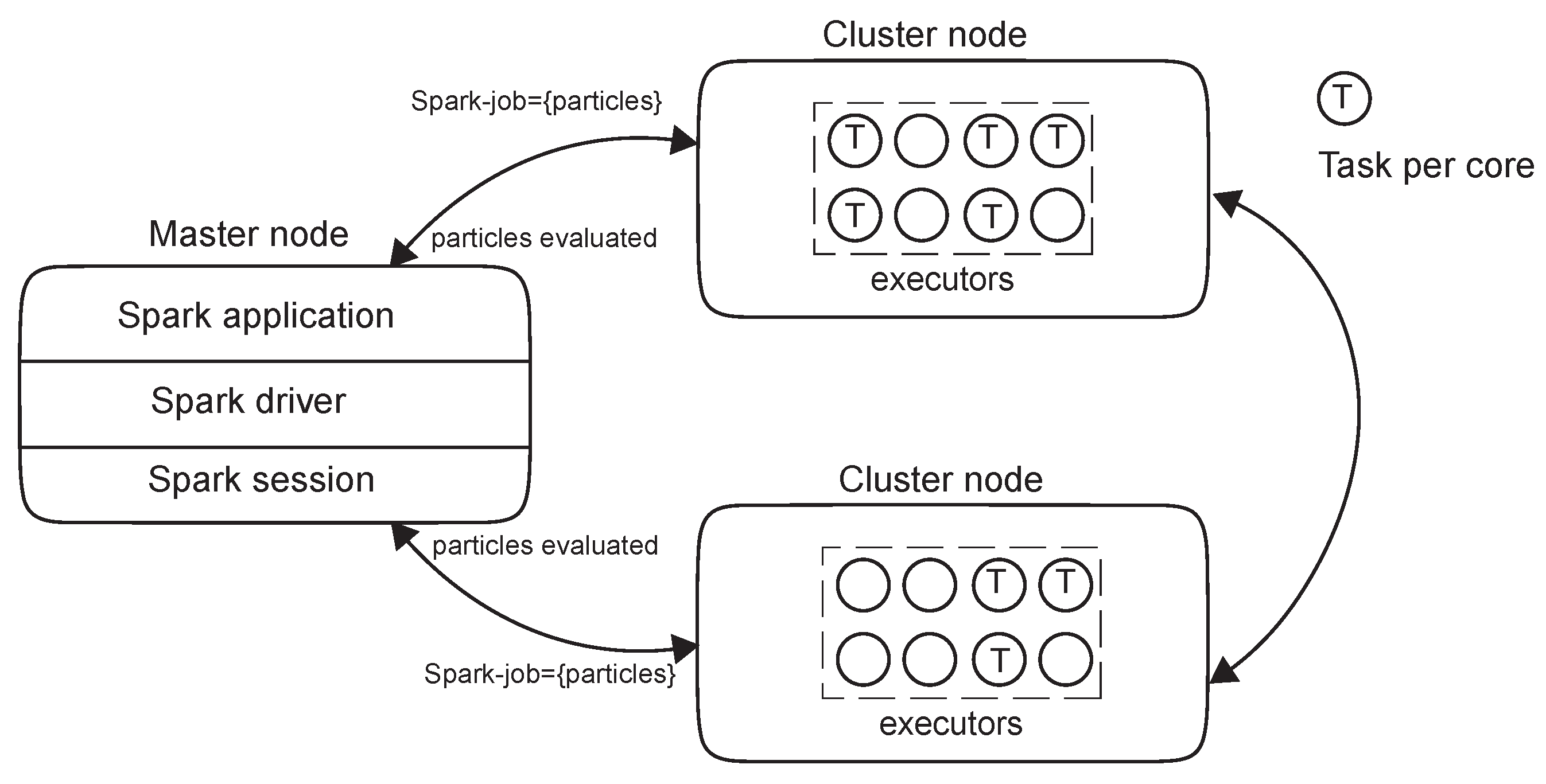
Figure 3.
Prediction with DSPSO implementation of the hourly power consumed during the month of January 2024 by a group of UGr buildings
Figure 3.
Prediction with DSPSO implementation of the hourly power consumed during the month of January 2024 by a group of UGr buildings
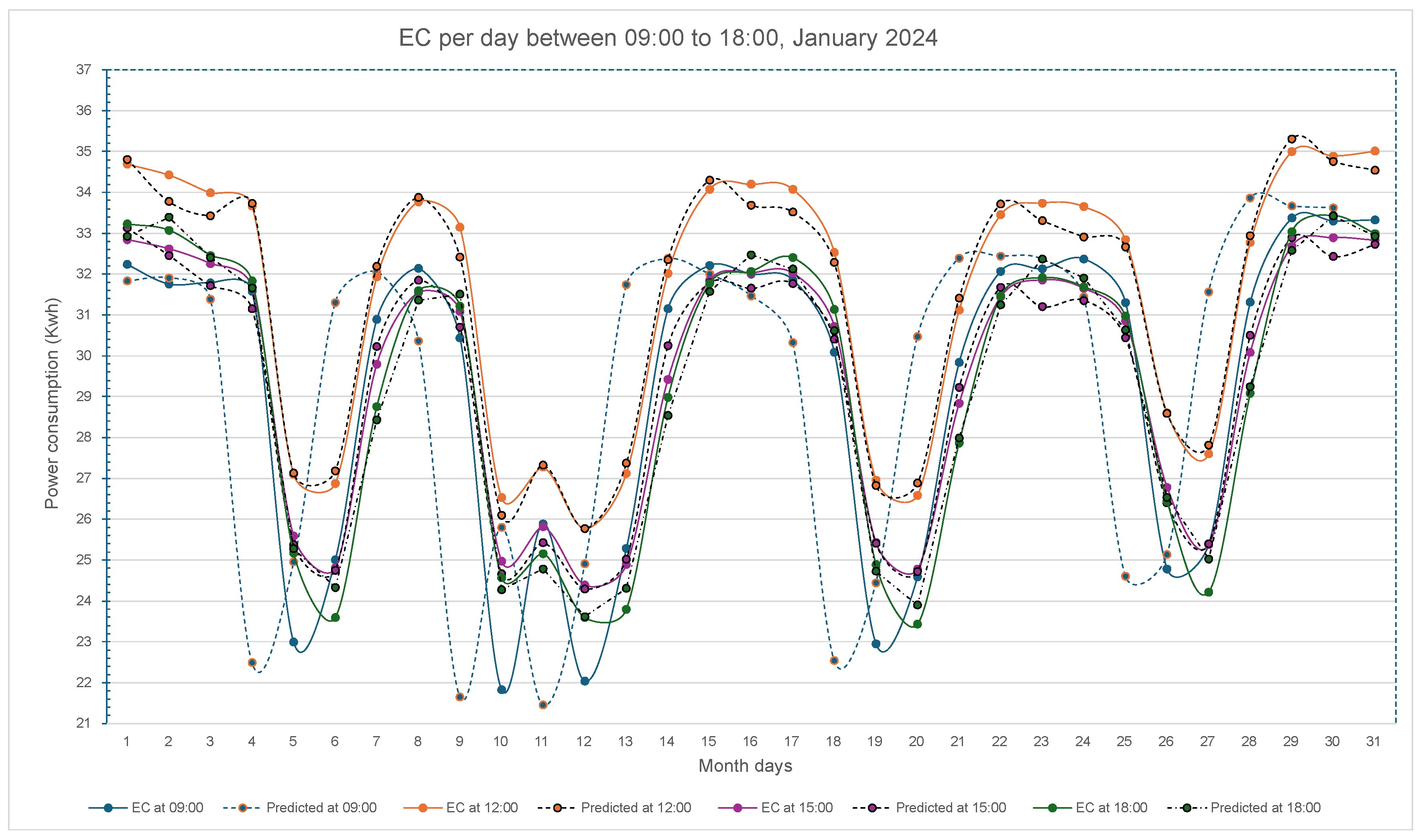
Figure 4.
Prediction with DAPSO implementation of the hourly power consumed during the month of January 2024 by a group of UGr buildings
Figure 4.
Prediction with DAPSO implementation of the hourly power consumed during the month of January 2024 by a group of UGr buildings
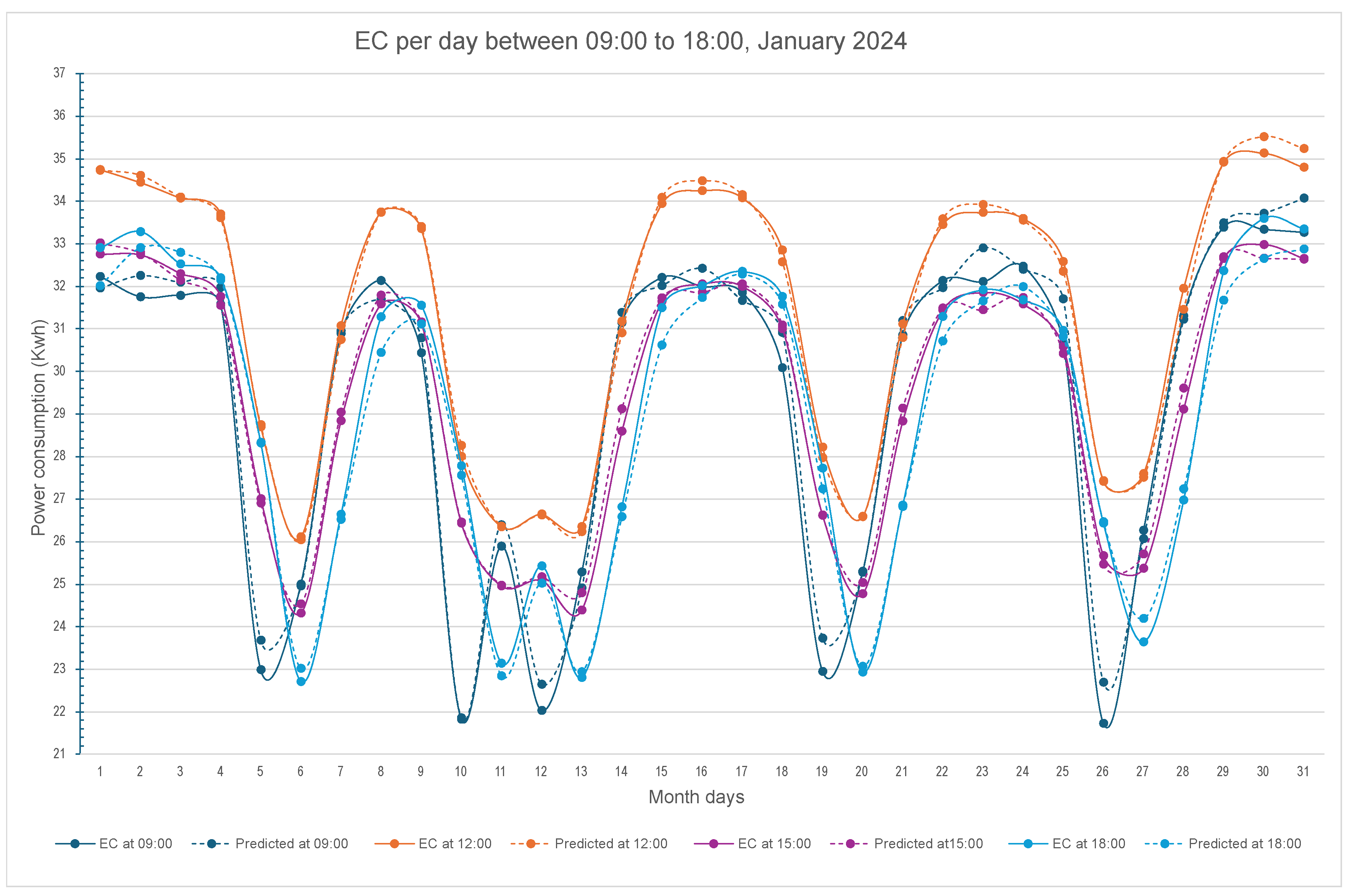
Figure 5.
Performance evaluation with change in the number of (a)particles, (b) iterations.
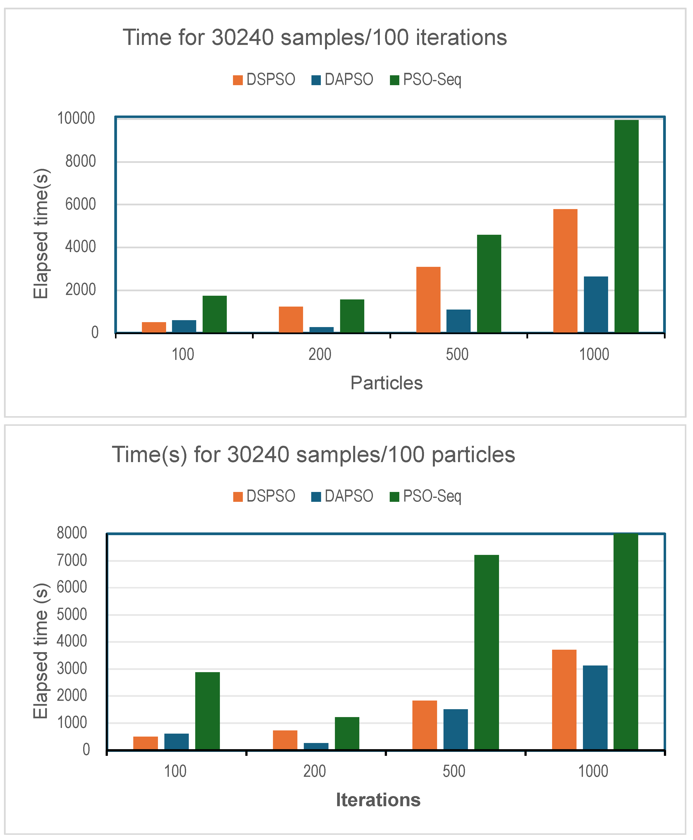
Figure 6.
Mean square error obtained with: (a)100 iterations, (b) 100 particles.
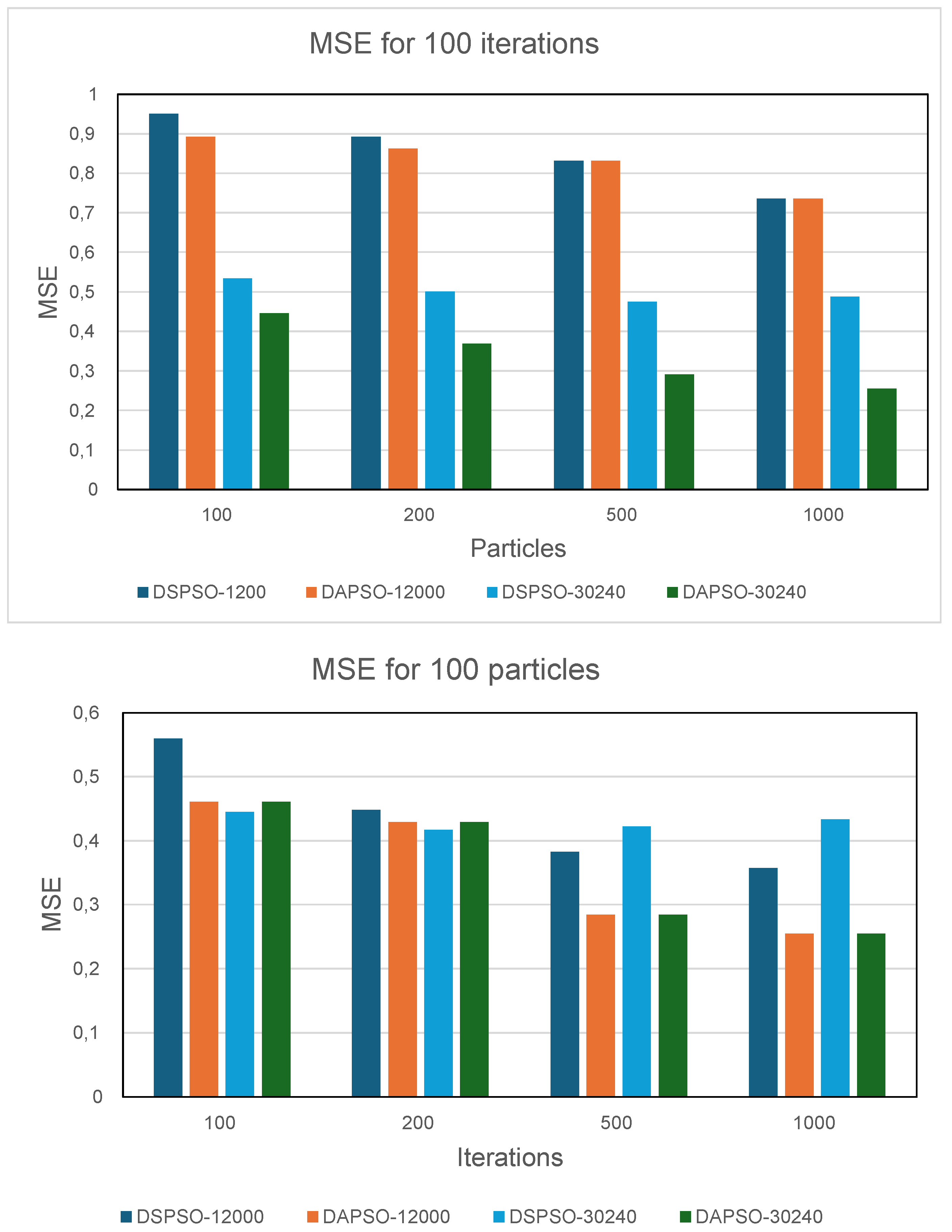
Figure 7.
Classification performance with (a) ROC curve, (b) precision/recall curve.
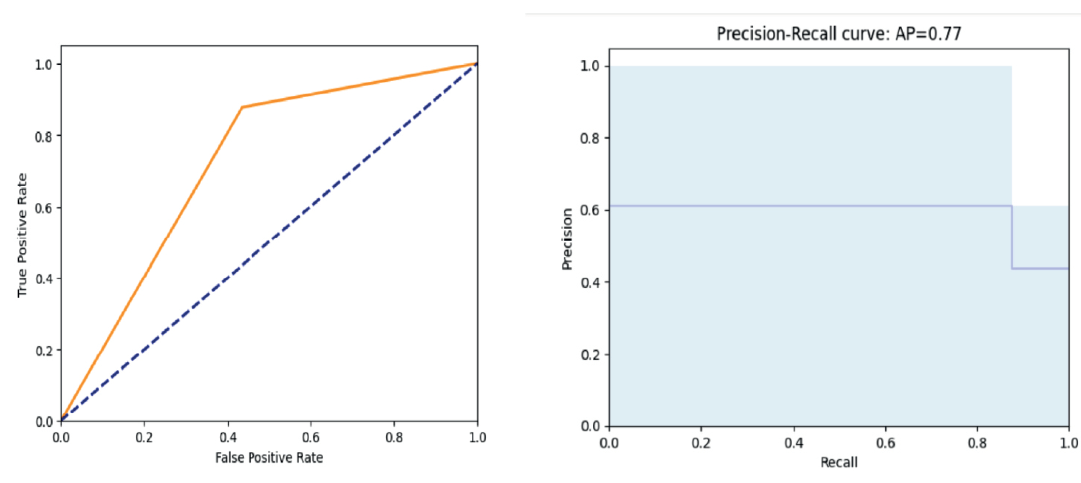
Table 2.
Parameter configuration for the EC prediction of a set of buildings for the DSPSO and DAPSO variants.
Table 2.
Parameter configuration for the EC prediction of a set of buildings for the DSPSO and DAPSO variants.
| Parameter | Value |
|---|---|
| Number of PSO iterations | 100, 200, 500, 1000 |
| Number of neurons in the input layer | 15 |
| Number of neurons in the hidden layer | 30 |
| Number of particles | 100, 200, 500, 1000 |
| SuperRDDs | 4 |
| Batch size | 10 |
| Interval of particle positions | [-1,1] |
| Particle velocity ranges | [-0.6,0.6] (0.6) |
| w | 1 |
| 0.8 | |
| 0.2 |
Table 3.
Chi-squared tests for each variable
| Variable | Chi-square value | P-value |
|---|---|---|
| height | 35178.19 | 0.0 |
| weight | 20419.24 | 0.0 |
| waist | 10849.84 | 0.0 |
| eyesight(left) | 2819.29 | 0.0 |
| eyesight(right) | 3432.92 | 0.0 |
| hearing(left) | 232.12 | 2.06e-52 |
| hearing(right) | 215.86 | 7.25e-49 |
| systolic | 1090.97 | 3.31e-236 |
| relaxation | 1875.90 | 0.0 |
| fasting blood sugar | 2089.03 | 0.0 |
| Cholesterol | 1215.51 | 3.16e-263 |
| triglyceride | 18319.41 | 0.0 |
| HDL | 10973.96 | 0.0 |
| LDL | 1067.00 | 5.24e-231 |
| hemoglobin | 34114.14 | 0.0 |
| Urine protein | 165.31 | 7.82e-38 |
| serum creatinine | 13429.07 | 0.0 |
| AST | 725.64 | 5.77e-157 |
| ALT | 7484.18 | 0.0 |
| Gtp | 26874.75 | 0.0 |
| dental caries | 1810.41 | 0.0 |
Table 4.
Odds Ratio for Categorical Variables
| Variable | Odds ratio |
|---|---|
| weight(kg)_Low | 0.20961654947072159 |
| weight(kg)_Medium_Low | 1.218644191656455 |
| weight(kg)_Medium_High | 2.097852237464934 |
| weight(kg)_High | 2.8299577733161576 |
| … | |
| fasting blood sugar_Low | 0.6308223587839904 |
| fasting blood sugar_Medium_Low | 0.9541383540661215 |
| fasting blood sugar_Medium_High | 1.173636730372843 |
| fasting blood sugar_High | 1.4547915548094907 |
| … | |
| triglyceride_Low | 0.23407715488962197 |
| triglyceride_Medium_Low | 0.7200827234227996 |
| triglyceride_Medium_High | 1.6370622749650663 |
| triglyceride_High | 3.1767870705800836 |
| HDL_Low | 2.365531709348869 |
| HDL_Medium_Low | 1.4317551296401139 |
| HDL_Medium_High | 0.7715794823329627 |
| HDL_High | 0.3282304510981655 |
| LDL_Low | 1.1629428483574764 |
| LDL_Medium_Low | 1.1890457266489936 |
| LDL_Medium_High | 1.0438026307432897 |
| LDL_High | 0.6844025582281992 |
| … | |
Table 5.
Relative Risk for Categorical Variables
| Variable | Relative Risk |
|---|---|
| weight(kg)_Low | 0.38230844375970974 |
| weight(kg)_Medium_Low | 1.1138572402084614 |
| weight(kg)_Medium_High | 1.4722921983586552 |
| weight(kg)_High | 1.657394753125524 |
| … | |
| fasting blood sugar_Low | 0.7625790496264635 |
| fasting blood sugar_Medium_Low | 0.9737980190980333 |
| fasting blood sugar_Medium_High | 1.0923983061205762 |
| fasting blood sugar_High | 1.2241433259236203 |
| … | |
| triglyceride_Low | 0.38822905484291464 |
| triglyceride_Medium_Low | 0.8257440932973402 |
| triglyceride_Medium_High | 1.2999795981567317 |
| triglyceride_High | 1.7644652462095984 |
| HDL_Low | 1.552294793364521 |
| HDL_Medium_Low | 1.21516619862005 |
| HDL_Medium_High | 0.8603055475766019 |
| HDL_High | 0.49401247683404703 |
| LDL_Low | 1.0871634378867505 |
| LDL_Medium_Low | 1.1002852299103176 |
| LDL_Medium_High | 1.0242964148293716 |
| LDL_High | 0.80065254077625 |
| … | |
Table 6.
Accuracy assessment of smoking Status using bio-Signals, with 10 and 100 particles and the 2 PSO variants.
Table 6.
Accuracy assessment of smoking Status using bio-Signals, with 10 and 100 particles and the 2 PSO variants.
| Classifier | Precision | Recall | F1-score | |||
|---|---|---|---|---|---|---|
| 10 | 100 | 10 | 100 | 10 | 100 | |
| DSPSO | 0.62 | 0.74 | 0.73 | 0.74 | 0.67 | 0.74 |
| DAPSO | 0.68 | 0.77 | 0.74 | 0.77 | 0.71 | 0.77 |
Table 7.
Performance of DSPSO and DAPSO on a Spark cluster with information on the number of executors and the number of blocks.
Table 7.
Performance of DSPSO and DAPSO on a Spark cluster with information on the number of executors and the number of blocks.
| DSPSO | DAPSO | |||
|---|---|---|---|---|
| # cores | 16 | 16 | ||
| Storage memory | 25 MiB | 135 KiB | ||
| Max. active tasks | 15 | 5 | ||
| Total number of created tasks | 2960 | 992 | ||
| Task execution (CPU) accumul. time | 28800 s. | 660 s. | ||
| Task execution (GPU) accumul. time | 384 s. | 7 s. | ||
| Average time of 1 parallel run | 1554 s. | 1060 s. | ||
Disclaimer/Publisher’s Note: The statements, opinions and data contained in all publications are solely those of the individual author(s) and contributor(s) and not of MDPI and/or the editor(s). MDPI and/or the editor(s) disclaim responsibility for any injury to people or property resulting from any ideas, methods, instructions or products referred to in the content. |
© 2024 by the authors. Licensee MDPI, Basel, Switzerland. This article is an open access article distributed under the terms and conditions of the Creative Commons Attribution (CC BY) license (https://creativecommons.org/licenses/by/4.0/).
Copyright: This open access article is published under a Creative Commons CC BY 4.0 license, which permit the free download, distribution, and reuse, provided that the author and preprint are cited in any reuse.


