Studying some Inequalities involving Polynomial Functions in π(x)

Subham De

doi:10.20944/preprints202407.1276.v1

Preprint

Article

Studying some Inequalities involving Polynomial Functions in π(x)

This version is not peer-reviewed.

Subham De^*

This version is not peer-reviewed.

Downloads

353

Views

170

Comments

Submitted:

15 July 2024

Posted:

16 July 2024

Read the latest preprint version here

Abstract

This article serves as a extensive research into proposing a few significant inequalities involving polynomial functions in $\pi(x)$, the \textit{prime counting function}, with an intention of exploring the behaviour of $\pi(x)$ for increasing $x$. The general case for such polynomials has also been discussed in detail towards the later section of the article, where the primary focus was to study the order of polynomials of the form, \begin{align*} P(\pi(x)) - \frac{e x}{\log x} Q(\pi(x/e)) + R(x) \end{align*} $P$, $Q$ and $R$ being arbitrary polynomials, and establish for a particular case that, the polynomial yields negative values for sufficiently large values of $x$. Furthermore, the error term in such estimations is of order $O\left(\frac{x^d}{(\log x)^{d+1}}\right)$, $d$ depends heavily upon $deg(P)$ and $deg(Q)$.

Keywords:

Arithmetic Function

;

Second Chebyshev Function

;

Prime Counting Function

;

Prime Number Theorem

;

Error Estimates

;

Polynomials

Subject:

Computer Science and Mathematics - Algebra and Number Theory

MSC: 11A41; 11A25; 11N05; 11N37; 11N56; 11M06; 11M26

1. Introduction and Motivation

The motivation for investigating the distribution of prime numbers over the real line

R

first reflected in the writings of famous mathematician Ramanujan, as evident from his letters [16] to one of the most prominent mathematician of 20^th century, G. H. Hardy during the months of Jan/Feb of 1913, which are testaments to several strong assertions about prime numbers, especaially the Prime Counting Function,

π (x)

[ref. (2.0.1)].

In the following years, Hardy himself analyzed some of thoose results [17] [18], and even wholeheartedly acknowledged about them in many of his publications, one such notable result is the Prime Number Theorem [ref. (3.4.1)].

Ramanujan provided several inequalities regarding the behaviour and the asymptotic nature of

π (x)

. One of such relation can be found in the notebooks written by Ramanujan himself has the following claim.

Theorem 1.0.1.(Ramanujan’s Inequality [2]) For x sufficiently large, we shall have,

\begin{matrix} {(π (x))}^{2} < \frac{e x}{log x} π (\frac{x}{e}) \end{matrix}

(1)

Worth mentioning that, Ramanujan indeed provided a simple, yet unique solution in support of his claim.

One immediate question which may pop up inside the head of any Number Theorist is that, what is meant by the term "large"? Apparently, over many years and even recently, a huge amount of effort has been put up by eminent researchers from all over the world in order to study Ramanujan’s Inequality, and focusing on understanding the behaviour of

π (x)

and any other Arithmetic Function associated to it. For example, it can be found in the work of Wheeler, Keiper, and Galway, Hassani[15]. Later on thanks to Dudek and Platt[3] and Axler[19], it has been well established that, a large proportion of posiive reals x falls under the category for which the inequality in fact is true.

This article serves as a humble tribute to arguably the most famous mathematician that there ever was, Srinivasa Ramanujan, and his stellar work on

π (x)

, where we shall derive a few important inequalities involving polynomial functions in

π (x)

, namely,

Cubic Polynomial Inequality
Higher-Degree Polynomial Inequality
Quadratic Form involving sums of Prime Counting Function, and,
Logarithmic Weighted Sum Inequality

We shall further discuss estimations for polynomials under a much more general setting in later section, although, one of the most important prospect of this article is justifying the equivalence of the statements of the Cubic Polynomial Inequality and Ramanujan’s Inequality. Important to highlight that, proper numerical verifications in support of justifying each and every inequality as proposed in section 3 have been thouroughly provided throughout the paper.

2. Important Derivations Regarding $π (x)$

We recall the definition of the Prime Counting Function [13,17] ,

π (x)

to be the number of primes less than or equal to

x \in R_{> 0}

. In addition to above, we further define the Second Chebyshev Function

ψ (x)

as follows.

Definition 2.0.1.

For every

x \geq 0

ψ (x) : = \sum_{n \leq x} Λ (n)

, Where,

Λ (n)

is the "Mangoldt Function" .

It can further be commented that [5],

\begin{matrix} ψ (x) = x + O (x^{1 / 2} {log}^{2} x) \end{matrix}

(2)

A priori a genius application of the Prime Number Theorem [13] allows us to obtain an estimate for

π (x)

in terms of

ψ (x)

Theorem 2.0.2.

\begin{matrix} π (x) = \frac{ψ (x)}{log x} + O (\frac{x}{{log}^{2} x}) \end{matrix}

(3)

Readers can refer to [5] in for a detailed solution of this result.

3. Inequalities Involving Polynomials in $π (x)$

3.1. Cubic Polynomial Inequality

The statement is as follows.

Theorem 3.1.1.

Let us consider the cubic polynomial of

π (x)

\begin{matrix} H (x) : = {(π (x))}^{3} - \frac{3 e x}{log x} {(π (x / e))}^{2} + \frac{3 e^{2} x}{{(log x)}^{2}} π (x / e^{2}) \end{matrix}

(4)

Given that

π (x)

is approximated by

\frac{x}{log x}

with a known error term, we can hypothesize that,

\begin{matrix} H (x) \approx O (\frac{x^{3}}{{(log x)}^{4}}) \end{matrix}

(5)

Furthermore,

H (x) < 0

for sufficiently large values of x.

Proof.

A priori from the order estimate between

π (x)

and

ψ (x)

as defined in (3) (cf. [5]), we compute the indivudual terms of

H (x)

as follows,

\begin{matrix} π (x / e) = \frac{ψ (x / e)}{log (x / e)} + O (\frac{x / e}{{(log (x / e))}^{2}}) = \frac{ψ (x / e)}{log x - 1} + O (\frac{x / e}{{(log x - 1)}^{2}}) \end{matrix}

(6)

and,

\begin{matrix} π (x / e^{2}) = \frac{ψ (x / e^{2})}{log (x / e^{2})} + O (\frac{x / e^{2}}{{(log (x / e^{2}))}^{2}}) = \frac{ψ (x / e^{2})}{log x - 2} + O (\frac{x / e^{2}}{{(log x - 2)}^{2}}) \end{matrix}

(7)

Furthermore,

\begin{matrix} {(π (x))}^{3} = {(\frac{ψ (x)}{log x} + O (\frac{x}{{(log x)}^{2}}))}^{3} = \frac{{(ψ (x))}^{3}}{{(log x)}^{3}} + 3 \cdot \frac{{(ψ (x))}^{2}}{{(log x)}^{3}} O (\frac{x}{{(log x)}^{2}}) \end{matrix}

\begin{matrix} + 3 \cdot \frac{ψ (x)}{{(log x)}^{3}} {(O (\frac{x}{{(log x)}^{2}}))}^{2} + {(O (\frac{x}{{(log x)}^{2}}))}^{3} \end{matrix}

(8)

Further simplification yields,

\begin{matrix} {(π (x))}^{3} = \frac{{(ψ (x))}^{3}}{{(log x)}^{3}} + O (\frac{x^{3}}{{(log x)}^{4}}) \end{matrix}

(9)

Finally,

\begin{matrix} \frac{3 e x}{log x} {(π (x / e))}^{2} = \frac{3 e x}{log x} {(\frac{ψ (x / e)}{log x - 1} + O (\frac{x / e}{{(log x - 1)}^{2}}))}^{2} \end{matrix}

\begin{matrix} = \frac{3 e x}{log x} (\frac{{(ψ (x / e))}^{2}}{{(log x - 1)}^{2}} + 2 \cdot \frac{ψ (x / e)}{{(log x - 1)}^{2}} O (\frac{x / e}{{(log x - 1)}^{2}}) + {(O (\frac{x / e}{{(log x - 1)}^{2}}))}^{2}) \end{matrix}

\begin{matrix} = \frac{3 e x {(ψ (x / e))}^{2}}{(log x) {(log x - 1)}^{2}} + O (\frac{x^{3}}{{(log x)}^{4}}) \end{matrix}

(10)

And,

\begin{matrix} \frac{3 e^{2} x}{{(log x)}^{2}} π (x / e^{2}) = \frac{3 e^{2} x}{{(log x)}^{2}} (\frac{ψ (x / e^{2})}{log x - 2} + O (\frac{x / e^{2}}{{(log x - 2)}^{2}})) \end{matrix}

\begin{matrix} = \frac{3 e^{2} x ψ (x / e^{2})}{{(log x)}^{2} (log x - 2)} + O (\frac{x^{3}}{{(log x)}^{4}}) \end{matrix}

(11)

Combining all the terms (6), (9), (10) and (11), we obtain,

\begin{matrix} H (x) = (\frac{{(ψ (x))}^{3}}{{(log x)}^{3}} + O (\frac{x^{3}}{{(log x)}^{4}})) - (\frac{3 e x {(ψ (x / e))}^{2}}{(log x) {(log x - 1)}^{2}} + O (\frac{x^{3}}{{(log x)}^{4}})) \end{matrix}

\begin{matrix} + (\frac{3 e^{2} x ψ (x / e^{2})}{{(log x)}^{2} (log x - 2)} + O (\frac{x^{3}}{{(log x)}^{4}})) \end{matrix}

Considering the dominant terms and the contributions of each term separately as compared to the error term, we get,

\begin{matrix} H (x) = \frac{{(ψ (x))}^{3}}{{(log x)}^{3}} - \frac{3 e x {(ψ (x / e))}^{2}}{(log x) {(log x - 1)}^{2}} + \frac{3 e^{2} x ψ (x / e^{2})}{{(log x)}^{2} (log x - 2)} + O (\frac{x^{3}}{{(log x)}^{4}}) \end{matrix}

(12)

Given the statement of the Prime Number Theorem [11][13],

ψ (x) \sim x

as x approaches ∞, thus we consider the dominant terms for sufficiently large x. Hence, substituting (2) in (12),

\begin{matrix} H (x) = \frac{x^{3}}{{(log x)}^{3}} - \frac{3 x^{3}}{e {(log x - 1)}^{3}} + \frac{3 x^{2}}{{(log x - 2)}^{3}} + O (\frac{x^{3}}{{(log x)}^{4}}) \end{matrix}

\begin{matrix} = - \frac{3 x^{3}}{e {(log x - 1)}^{3}} + O (\frac{x^{3}}{{(log x)}^{4}}) \end{matrix}

(13)

Since,

\frac{3 x^{3}}{e {(log x - 1)}^{3}} > 0

for sufficiently large x ( observe that higher-order terms diminish as x grows ), the dominant term is thus negative.

In coclusion, for sufficiently large values of x, one shall have (5) to satisfy and,

H (x) < 0

. □

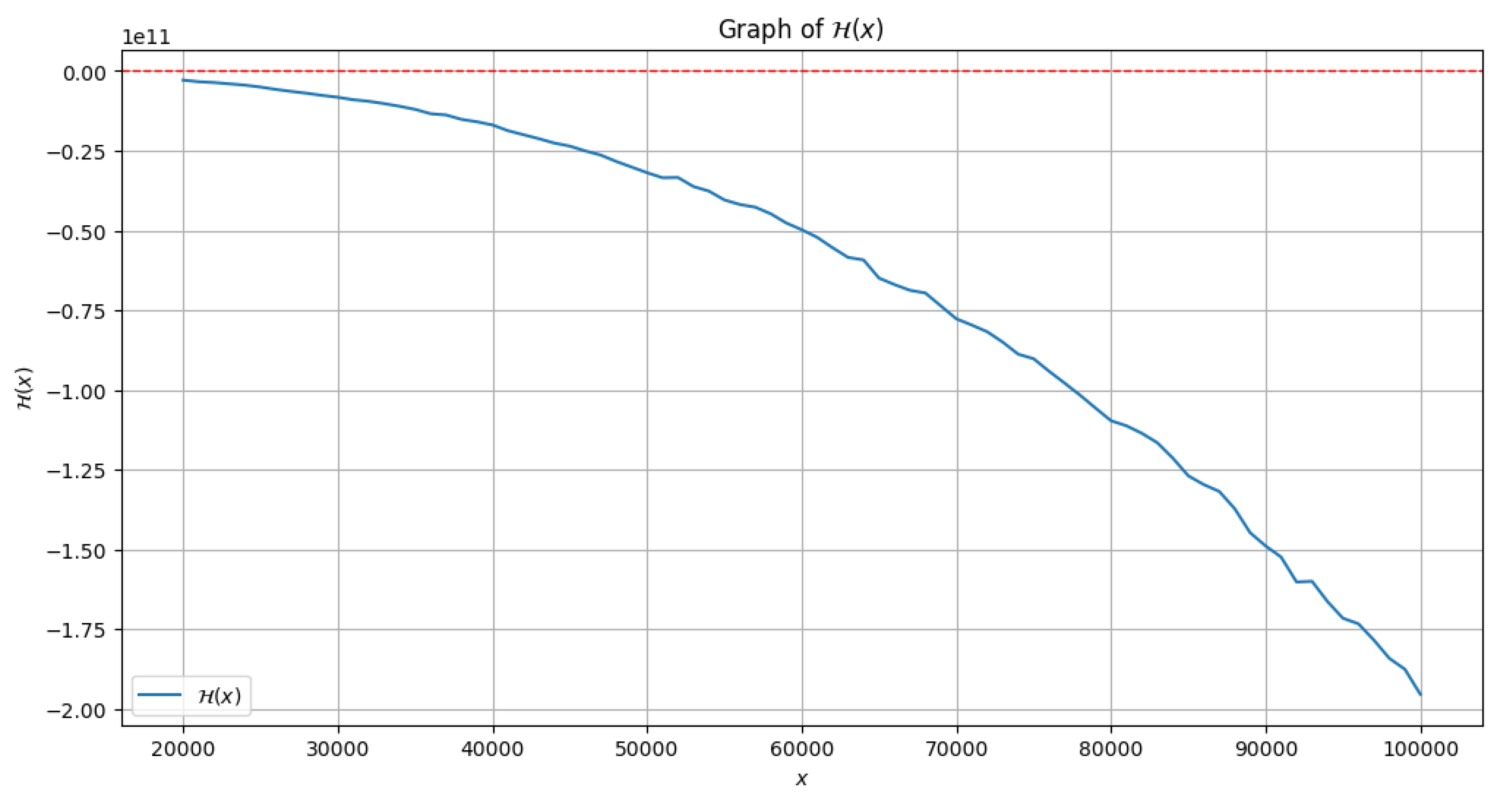
Remark 3.1.2. In other words, the Cubic polynomial Inequality can be reformulated as,

\begin{matrix} {(π (x))}^{3} + \frac{3 e^{2} x}{{(log x)}^{2}} π (x / e^{2}) < \frac{3 e x}{log x} {(π (x / e))}^{2} \end{matrix}

(14)

for sufficiently large values of x.

Important to note that, one can utilize Mathematica in order to observe the plot of

H (x)

as compared to x. The following Figure shows the graph for

2 \times 10^{4} \leq x \leq 10^{5}

. Furthermore, rigorous computation yields the following values of

H (x)

as mentioned in Table 1 in the range,

10^{4} \leq x \leq 10^{18}

. The data clearly suggests that, the function

H (x)

is indeed decreasing in this interval, hence, our claim (14) can also be justified numerically.

Figure 1.

3.2. Higher-Degree Polynomial Inequality

Theorem 3.2.1.

For higher powers, let’s consider,

\begin{matrix} K (x) : = {(π (x))}^{4} - \frac{4 e x}{log x} {(π (x / e))}^{3} + \frac{6 e^{2} x}{{(log x)}^{2}} {(π (x / e^{2}))}^{2} - \frac{4 e^{3} x}{{(log x)}^{3}} π (x / e^{3}) \end{matrix}

(15)

Then, the following holds true,

\begin{matrix} K (x) \approx O (\frac{x^{4}}{{(log x)}^{5}}) \end{matrix}

(16)

and for sufficiently large x we have,

K (x) > 0

Proof.

A priori using the relation (3) (cf. [5]) from Theorem (2.0.2), along with (6) and (7),

\begin{matrix} π (x / e^{3}) = \frac{ψ (x / e^{3})}{log x - 3} + O (\frac{x / e^{3}}{{(log x - 3)}^{2}}) \end{matrix}

(17)

Now, we compute,

\begin{matrix} {(π (x))}^{4} = {(\frac{ψ (x)}{log x} + O (\frac{x}{{(log x)}^{2}}))}^{4} = \frac{{(ψ (x))}^{4}}{{(log x)}^{4}} + O (\frac{x^{4}}{{(log x)}^{5}}) \end{matrix}

(18)

Moreover,

\begin{matrix} \frac{4 e x}{log x} {(π (x / e))}^{3} = \frac{4 e x}{log x} {(\frac{ψ (x / e)}{log x - 1} + O (\frac{x / e}{{(log x - 1)}^{2}}))}^{3} = \frac{4 e x {(ψ (x / e))}^{3}}{(log x) {(log x - 1)}^{3}} + O (\frac{x^{4}}{{(log x)}^{5}}) \end{matrix}

(19)

Subsequently, we approximate the rest of the terms of

K (x)

as follows.

\begin{matrix} \frac{6 e^{2} x}{{(log x)}^{2}} {(π (x / e^{2}))}^{2} = \frac{6 e^{2} x}{{(log x)}^{2}} {(\frac{ψ (x / e^{2})}{log x - 2} + O (\frac{x / e^{2}}{{(log x - 2)}^{2}}))}^{2} \end{matrix}

\begin{matrix} = \frac{6 e^{2} x {(ψ (x / e^{2}))}^{2}}{{(log x)}^{2} {(log x - 2)}^{2}} + O (\frac{x^{4}}{{(log x)}^{5}}) \end{matrix}

(20)

And,

\begin{matrix} \frac{4 e^{3} x}{{(log x)}^{3}} π (x / e^{3}) = \frac{4 e^{3} x}{{(log x)}^{3}} (\frac{ψ (x / e^{3})}{log x - 3} + O (\frac{x / e^{3}}{{(log x - 3)}^{2}})) \end{matrix}

\begin{matrix} = \frac{4 e^{3} x ψ (x / e^{3})}{{(log x)}^{3} (log x - 3)} + O (\frac{x^{4}}{{(log x)}^{5}}) \end{matrix}

(21)

Combining (17), (18), (19), (20) and (21), and sorting out the dominant terms and their contributions towards the error term,

\begin{matrix} K (x) = \frac{{(ψ (x))}^{4}}{{(log x)}^{4}} - \frac{4 e x {(ψ (x / e))}^{3}}{(log x) {(log x - 1)}^{3}} + \frac{6 e^{2} x {(ψ (x / e^{2}))}^{2}}{{(log x)}^{2} {(log x - 2)}^{2}} - \frac{4 e^{3} x ψ (x / e^{3})}{{(log x)}^{3} (log x - 3)} + O (\frac{x^{4}}{{(log x)}^{5}}) \end{matrix}

(22)

A simple application of (2) yields,

\begin{matrix} K (x) = \frac{x^{4}}{{(log x)}^{4}} - \frac{4 e x x^{3}}{{(log x)}^{4}} + \frac{6 e^{2} x x^{2}}{{(log x)}^{4}} - \frac{4 e^{3} x x}{{(log x)}^{4}} + O (\frac{x^{4}}{{(log x)}^{5}}) \end{matrix}

\begin{matrix} = \frac{x^{4}}{{(log x)}^{4}} (1 - \frac{4 e}{log x} + \frac{6 e^{2}}{{(log x)}^{2}} - \frac{4 e^{3}}{{(log x)}^{3}}) + O (\frac{x^{4}}{{(log x)}^{5}}) \end{matrix}

(23)

Since

(1 - \frac{4 e}{log x} + \frac{6 e^{2}}{{(log x)}^{2}} - \frac{4 e^{3}}{{(log x)}^{3}})

is positive for sufficiently large x (higher-order terms diminish as x grows), hence the dominant term is positive. Accordingly, the error term in the approximation is,

\begin{matrix} O (\frac{x^{4}}{{(log x)}^{5}}) \end{matrix}

In conclusion, we assert that, (16) indeed holds true, and

K (x) > 0

for sufficiently large enough x. □

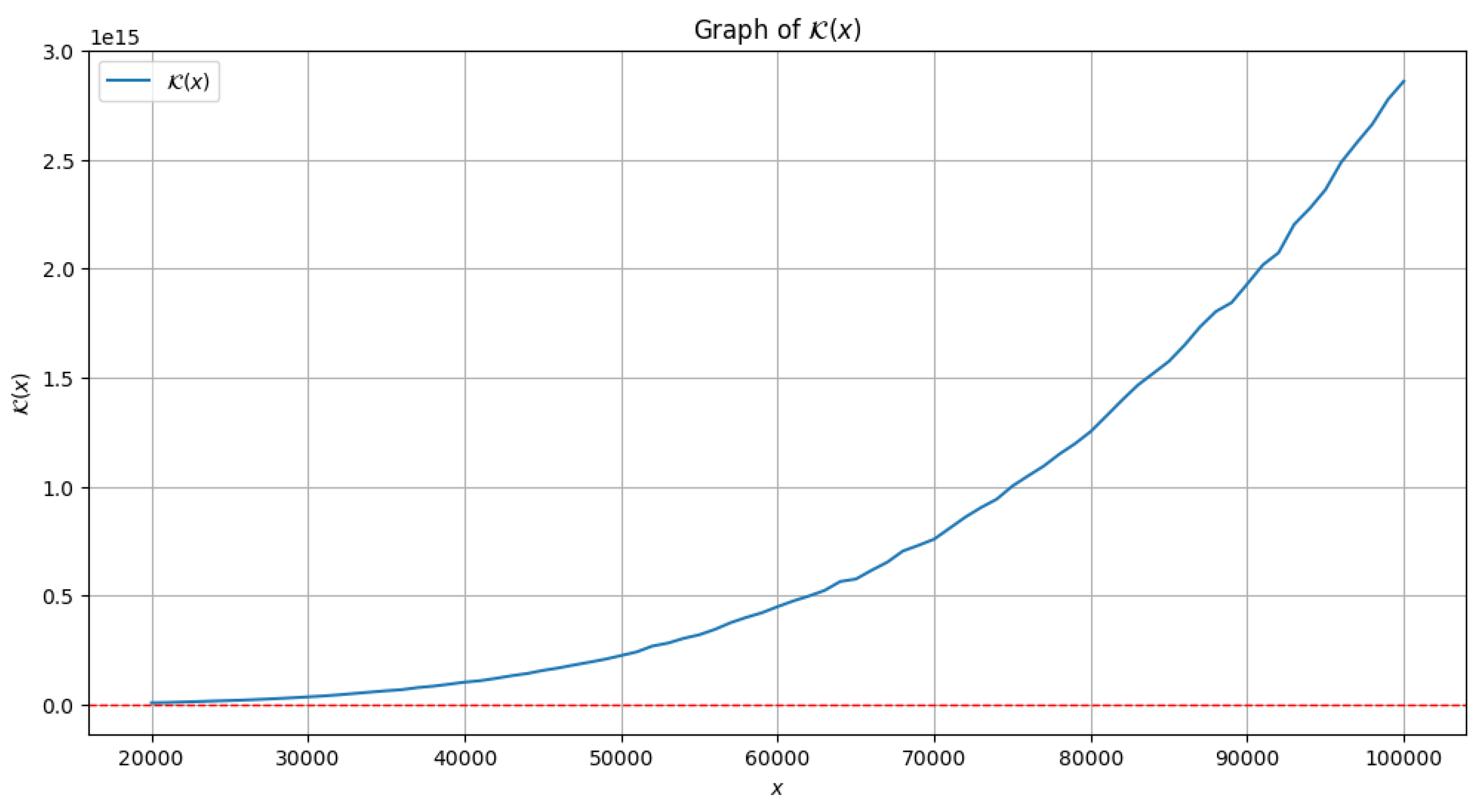
Remark 3.2.2. We can also rephrase the result obtained from Theorem (3.2.1) in the form,

\begin{matrix} \frac{4 e x}{log x} {(π (x / e))}^{3} + \frac{4 e^{3} x}{{(log x)}^{3}} π (x / e^{3}) < {(π (x))}^{4} + \frac{6 e^{2} x}{{(log x)}^{2}} {(π (x / e^{2}))}^{2} \end{matrix}

(24)

for sufficiently large values of x.

Important to observe that, one can apply Mathematica in order to observe the plot of

K (x)

as compared to x. The following Figure shows the plot for

2 \times 10^{4} \leq x \leq 10^{5}

.Moreover, the following values of

H (x)

can in fact be calculated as evident from Table 2 in the range,

10^{4} \leq x \leq 10^{17}

. Using the data one can clearly infer that,

K (x)

is indeed increasing in this interval, hence, our claim (24) can be established numerically.

Figure 2.

3.3. Quadratic Form Involving Sums of Prime Counting Function

Theorem 3.3.1.

Consider a quadratic form involving the sum of the prime counting function over smaller intervals,

\begin{matrix} L (x) = {(\sum_{k = 1}^{n} π (x / k))}^{2} - \frac{e x}{log x} (\sum_{k = 1}^{n} π (x / (e k))), n > 1 \end{matrix}

(25)

For some fixed n, then we have the following approximation,

\begin{matrix} L (x) \approx O (\frac{x^{2}}{{(log x)}^{2}}) \end{matrix}

(26)

With

L (x) > 0

for sufficiently large values of x.

Proof.

For the proof, we evaluate terms inside the summand of

L (x)

, a priori using the result (3) (cf. [5]) in Theorem (2.0.2).

\begin{matrix} π (x / k) = \frac{ψ (x / k)}{log x - log k} + O (\frac{x / k}{{(log x - log k)}^{2}}) \end{matrix}

(27)

\begin{matrix} π (x / (e k)) = \frac{ψ (x / (e k))}{log x - log (e k)} + O (\frac{x / (e k)}{{(log x - log (e k))}^{2}}) \end{matrix}

(28)

Hence,

\begin{matrix} \sum_{k = 1}^{n} π (x / k) = \sum_{k = 1}^{n} (\frac{ψ (x / k)}{log x - log k} + O (\frac{x / k}{{(log x - log k)}^{2}})) \end{matrix}

\begin{matrix} = \sum_{k = 1}^{n} \frac{ψ (x / k)}{log x - log k} + O (\sum_{k = 1}^{n} \frac{x / k}{{(log x - log k)}^{2}}) \end{matrix}

(29)

Similarly,

\begin{matrix} \sum_{k = 1}^{n} π (x / (e k)) = \sum_{k = 1}^{n} (\frac{ψ (x / (e k))}{log x - log (e k)} + O (\frac{x / (e k)}{{(log x - log (e k))}^{2}})) \end{matrix}

\begin{matrix} = \sum_{k = 1}^{n} \frac{ψ (x / (e k))}{log x - log (e k)} + O (\sum_{k = 1}^{n} \frac{x / (e k)}{{(log x - log (e k))}^{2}}) \end{matrix}

(30)

Squaring (29) gives,

\begin{matrix} {(\sum_{k = 1}^{n} π (x / k))}^{2} = {(\sum_{k = 1}^{n} \frac{ψ (x / k)}{log x - log k} + O (\sum_{k = 1}^{n} \frac{x / k}{{(log x - log k)}^{2}}))}^{2} \approx {(\sum_{k = 1}^{n} \frac{ψ (x / k)}{log x - log k})}^{2} \end{matrix}

Ignoring the higher-order terms for the time being. Further computation yields,

\begin{matrix} {(\sum_{k = 1}^{n} \frac{ψ (x / k)}{log x - log k})}^{2} = \sum_{k = 1}^{n} \sum_{j = 1}^{n} \frac{ψ (x / k) ψ (x / j)}{(log x - log k) (log x - log j)} \end{matrix}

(31)

Combining (30) and (31),

\begin{matrix} L (x) \approx {(\sum_{k = 1}^{n} \frac{ψ (x / k)}{log x - log k})}^{2} - \frac{e x}{log x} \sum_{k = 1}^{n} \frac{ψ (x / (e k))}{log x - log (e k)} \end{matrix}

(32)

An important observation is that, the leading term of

ψ (x)

is x, so for large x,

\begin{matrix} ψ (x / k) = \frac{x}{k} + O (\sqrt{\frac{x}{k}} {log}^{2} x) \end{matrix}

and,

\begin{matrix} ψ (x / (e k)) = \frac{x}{e k} + O (\sqrt{\frac{x}{e k}} {log}^{2} x) \end{matrix}

Therefore, using the leading term approximation, we can deduce,

\begin{matrix} L (x) \approx {(\sum_{k = 1}^{n} \frac{x / k}{log x - log k})}^{2} - \frac{e x}{log x} \sum_{k = 1}^{n} \frac{x / (e k)}{log x - log (e k)} \end{matrix}

Where,

\begin{matrix} {(\sum_{k = 1}^{n} \frac{x / k}{log x - log k})}^{2} \approx {(\frac{x}{log x} \sum_{k = 1}^{n} \frac{1}{k})}^{2} \approx {(\frac{x}{log x} H_{n})}^{2} \end{matrix}

H_{n}

denoting the n-th Harmonic Number,

H_{n} \approx log n + γ

γ

being the Euler Constant.

As for the second term in the expression of

L (x)

\begin{matrix} \frac{e x}{log x} \sum_{k = 1}^{n} \frac{x / (e k)}{log x - log (e k)} \approx \frac{e x}{log x} \cdot \frac{x}{e log x} \sum_{k = 1}^{n} \frac{1}{k} \approx {(\frac{x}{log x})}^{2} H_{n} \end{matrix}

Therefore,

\begin{matrix} L (x) \approx {(\frac{x H_{n}}{log x})}^{2} - \frac{x^{2} H_{n}}{{(log x)}^{2}} \approx \frac{x^{2} {(log n)}^{2}}{{(log x)}^{2}} - \frac{x^{2} log n}{{(log x)}^{2}} \approx \frac{x^{2} log n (log n - 1)}{{(log x)}^{2}} \end{matrix}

On the other hand, analyzing the error terms from previously derived estimates, it can be deduced that,

\begin{matrix} L (x) = O (\frac{x^{2}}{{(log x)}^{2}}) \end{matrix}

(33)

Hence, (26) follows. Moreover, since the leading term

\frac{x^{2} log n (log n - 1)}{{(log x)}^{2}}

is positive for

n > 1

, thus it implies that

L (x)

is positive for large x, and the proof is complete. □

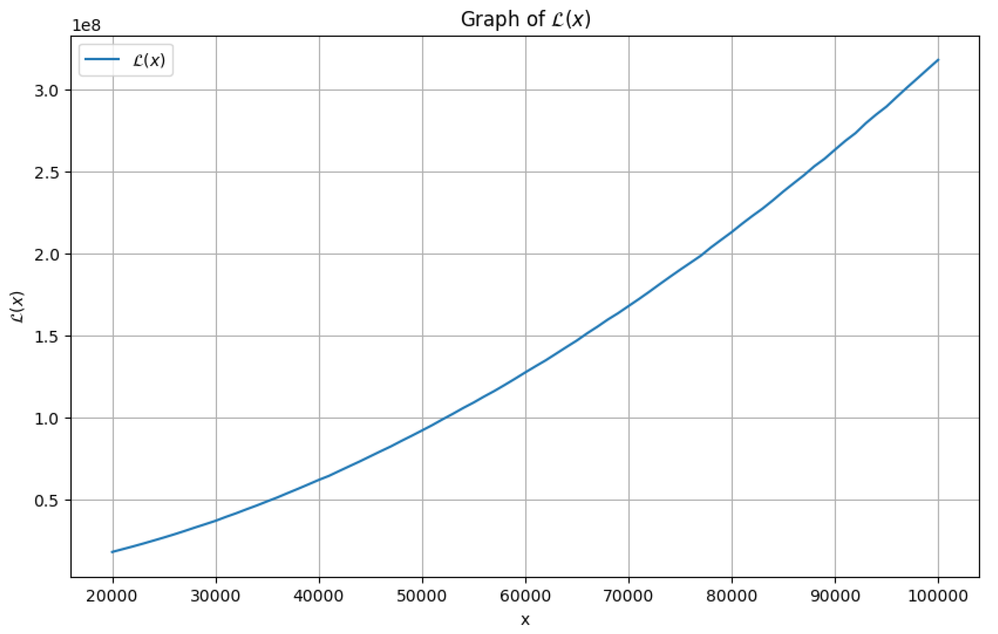
Remark 3.3.2. We can rephrase Theorem (3.3.1) by claiming that, for every

n > 1

\begin{matrix} {(\sum_{k = 1}^{n} π (x / k))}^{2} > \frac{e x}{log x} (\sum_{k = 1}^{n} π (x / (e k))) \end{matrix}

(34)

for sufficiently large x.

For a specific scenario when

n = 5

, plotting

L (x)

as compared to x using Mathematica gives us the following graph as in Figure for

2 \times 10^{4} \leq x \leq 10^{5}

. Moreover, it can be asserted using the data shown in Table 3 in the range,

10^{4} \leq x \leq 10^{16}

that,

L (x)

is indeed increasing. As a result, the statement (34) can be properly accepted.

Figure 3.

3.4. Logarithmic Weighted Sum Inequality

It is very much possible to improve (26) even further, where one can also consider the case which involves logarithmic weights.

Theorem 3.4.1.

The following can in fact be conjectured for the logarithmic weights,

\begin{matrix} F (x) : = {(\sum_{k = 1}^{n} \frac{π (x / k)}{log (x / k)})}^{2} - \frac{e x}{log x} (\sum_{k = 1}^{n} \frac{π (x / (e k))}{log (x / (e k))}), n > 1 \end{matrix}

(35)

Then,

\begin{matrix} F (x) \approx O (\frac{x^{2}}{{(log x)}^{3}}) \end{matrix}

(36)

And,

F (x) < 0

for large values of x.

Proof.

A priori for large x, utilizing (2) (cf. [5]),

\begin{matrix} ψ (x / k) = \frac{x}{k} + O (\sqrt{\frac{x}{k}} {log}^{2} (\frac{x}{k})) \end{matrix}

and,

\begin{matrix} ψ (x / (e k)) = \frac{x}{e k} + O (\sqrt{\frac{x}{e k}} {log}^{2} (\frac{x}{e k})) \end{matrix}

Rigorously computation each and every term of

F (x)

yields,

\begin{matrix} \sum_{k = 1}^{n} \frac{π (x / k)}{log (x / k)} = \sum_{k = 1}^{n} (\frac{ψ (x / k)}{{(log (x / k))}^{2}} + O (\frac{x / k}{{(log (x / k))}^{3}})), \end{matrix}

(37)

and similarly,

\begin{matrix} \sum_{k = 1}^{n} \frac{π (x / (e k))}{log (x / (e k))} = \sum_{k = 1}^{n} (\frac{ψ (x / (e k))}{{(log (x / (e k)))}^{2}} + O (\frac{x / (e k)}{{(log (x / (e k)))}^{3}})) . \end{matrix}

(38)

Subsequently squaring the left-hand side of (37),

\begin{matrix} {(\sum_{k = 1}^{n} \frac{π (x / k)}{log (x / k)})}^{2} = {(\sum_{k = 1}^{n} (\frac{ψ (x / k)}{{(log (x / k))}^{2}}) + \sum_{k = 1}^{n} O (\frac{x / k}{{(log (x / k))}^{3}}))}^{2} \end{matrix}

Using the Cauchy-Schwarz Inequality, and considering the main term and error terms separately,

\begin{matrix} {(\sum_{k = 1}^{n} \frac{x}{k {(log (x / k))}^{2}})}^{2} = \frac{x^{2}}{{(log x)}^{4}} {(\sum_{k = 1}^{n} \frac{1}{k})}^{2} = \frac{x^{2}}{{(log x)}^{4}} {(H_{n})}^{2} \end{matrix}

(39)

Where,

H_{n}

denotes the Harmonic Number. Using the harmonic series approximation,

\begin{matrix} H_{n} = \sum_{k = 1}^{n} \frac{1}{k} \approx log n + γ . \end{matrix}

(40)

Hence, from (39),

\begin{matrix} {(\sum_{k = 1}^{n} \frac{π (x / k)}{log (x / k)})}^{2} = \frac{x^{2} {log}^{2} n}{{(log x)}^{4}} . \end{matrix}

(41)

As for the error term,

\begin{matrix} O (\sum_{k = 1}^{n} \frac{x / k}{{(log (x / k))}^{3}}) = O (\sum_{k = 1}^{n} \frac{x / k}{{(log (x / k))}^{3}}) = O (\frac{x log n}{{(log x)}^{3}}) \end{matrix}

Thus, combining all our deductions,

\begin{matrix} {(\sum_{k = 1}^{n} \frac{π (x / k)}{log (x / k)})}^{2} = \frac{x^{2} {log}^{2} n}{{(log x)}^{4}} + O (\frac{x^{2} {log}^{2} n}{{(log x)}^{6}}) \end{matrix}

Furthermore, for the second term in (35), we have the following calculations,

\begin{matrix} \frac{e x}{log x} \sum_{k = 1}^{n} \frac{π (x / (e k))}{log (x / (e k))} = \frac{e x}{log x} \sum_{k = 1}^{n} (\frac{ψ (x / (e k))}{{(log (x / (e k)))}^{2}} + O (\frac{x / (e k)}{{(log (x / (e k)))}^{3}})) . \end{matrix}

(42)

Approximating the main term,

\begin{matrix} \frac{e x}{log x} \sum_{k = 1}^{n} \frac{x / (e k)}{{(log (x / (e k)))}^{2}} = \frac{e x^{2}}{log x} \sum_{k = 1}^{n} \frac{1}{e k {(log (x / (e k)))}^{2}} \end{matrix}

Using the harmonic series approximation,

\begin{matrix} \sum_{k = 1}^{n} \frac{1}{e k} \approx \frac{log n}{e} \end{matrix}

As a consequence,

\begin{matrix} \frac{e x^{2}}{log x} \frac{log n}{e {(log x)}^{2}} = \frac{x^{2} log n}{{(log x)}^{3}} . \end{matrix}

Combining all,

\begin{matrix} F (x) = {(\sum_{k = 1}^{n} \frac{π (x / k)}{log (x / k)})}^{2} - \frac{e x}{log x} (\sum_{k = 1}^{n} \frac{π (x / (e k))}{log (x / (e k))}) \end{matrix}

\begin{matrix} = \frac{x^{2} {log}^{2} n}{{(log x)}^{4}} + O (\frac{x^{2} {log}^{2} n}{{(log x)}^{6}}) - \frac{x^{2} log n}{{(log x)}^{3}} = - \frac{x^{2} log n}{{(log x)}^{3}} + O (\frac{x^{2} log n}{{(log x)}^{4}}) \end{matrix}

Considering the dominant term. As a result, we conclude,

\begin{matrix} F (x) \approx O (\frac{x^{2} log n}{{(log x)}^{4}}) = O (\frac{x^{2}}{{(log x)}^{3}}) \end{matrix}

for large x, and moreover, the dominant term,

\frac{x^{2} log n}{{(log x)}^{3}}

being always positive for

n > 1

, we can thus assert that,

F (x) < 0

for sufficiently large values of x. □

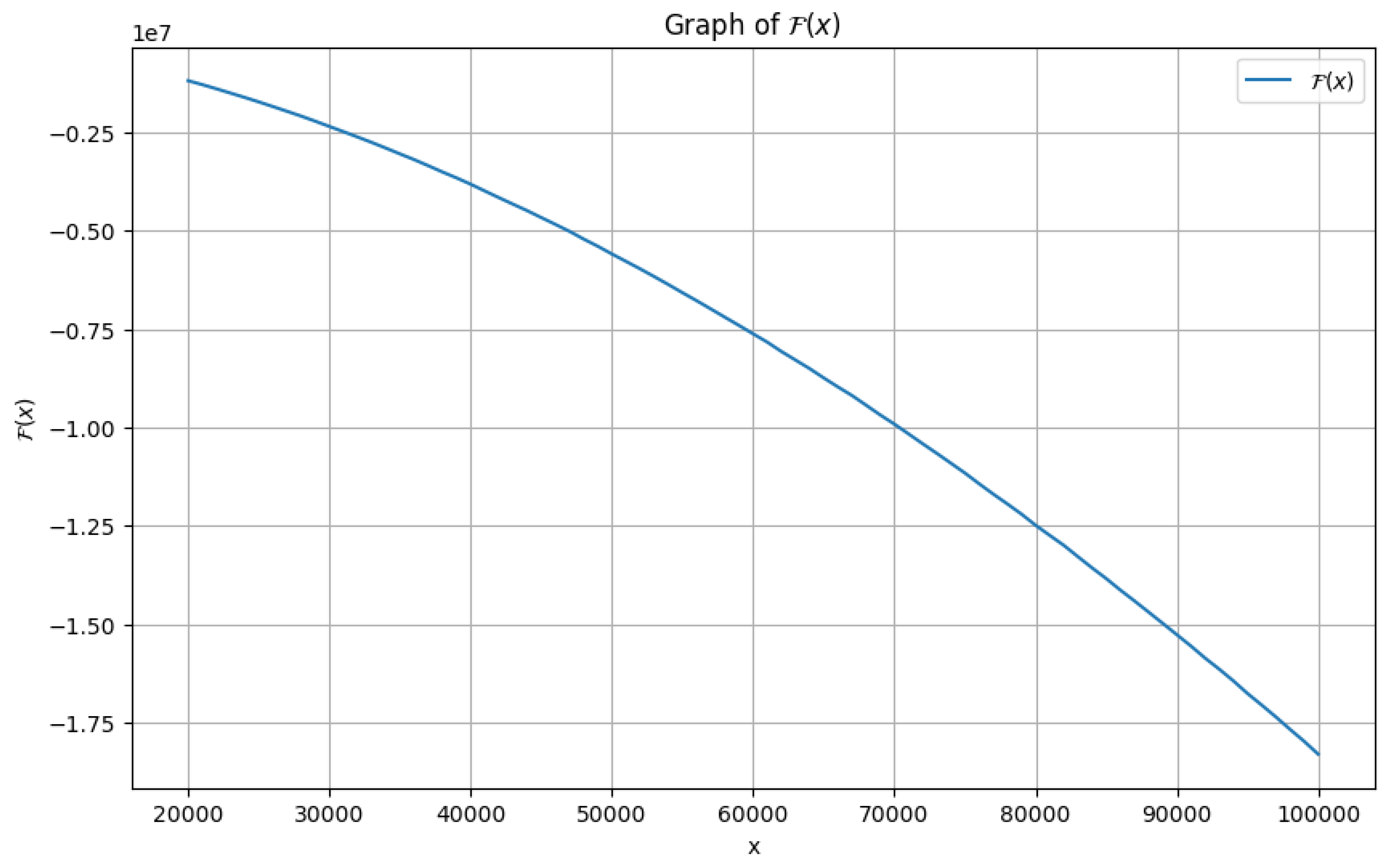
Remark 3.4.2. We can reaffirm Theorem (3.4.1) in the following manner. For any

n > 1

\begin{matrix} {(\sum_{k = 1}^{n} \frac{π (x / k)}{log (x / k)})}^{2} < \frac{e x}{log x} (\sum_{k = 1}^{n} \frac{π (x / (e k))}{log (x / (e k))}) \end{matrix}

(43)

for sufficiently large values of x.

Similarly as in other cases, Mathematica can in fact be applied in order to observe the plot of

F (x)

as compared to x. The following Figure shows the graph for

2 \times 10^{4} \leq x \leq 10^{5}

and considering

n = 5

In addition to above, it can be observed in Table 4 that,

F (x)

is in fact decreasing in the range,

10^{4} \leq x \leq 10^{14}

. As a result, the statement (43) can also be numerically verified for large values of x.

Figure 4.

4. A More General Framework

Given the asymptotic nature of the prime counting function

π (x)

, the general form of such inequalities can be formulated as follows.

\begin{matrix} N (x) : = P (π (x)) - \frac{e x}{log x} Q (π (x / e)) + R (x) \end{matrix}

(44)

where P and Q are polynomials and R is a term that compensates for higher-order error terms. Subsequently, one can claim that, the error term in (44) might behave similarly as in the previous cases. In mathematical terms, it might very well be possible that,

\begin{matrix} N (x) \approx O (\frac{x^{d}}{{(log x)}^{d + 1}}) \end{matrix}

(45)

for some degree d depending on the degrees of P and Q.

4.1. A Typical Example

In order to justify our claim (45) corresponding to (44), let’s delve into a specific example by explicitly choosing polynomials P, Q, and

R (x)

and studying the function

N (x)

for different cases explicitely.

Consider the polynomials,

\begin{matrix} P (π (x)) = Q (π (x)) = {(\sum_{k = 1}^{n} π (x / k))}^{r} \end{matrix}

To maintain symmetry and include higher-order error terms, we choose

R (x) = {(\sum_{k = 1}^{n} π (x / (e^{2} k)))}^{r}

. It can be observed that, degrees of each of the polynomials P, Q and R are the same

= r

. We study the polynomial

N_{r} (x)

under two circumstances separately.

4.1.1. deg(P), deg(Q) and deg(R) Are Odd

We assume,

r = 2 m + 1

, for any positive integer m. As a result, the polynomial takes the form,

\begin{matrix} N_{2 m + 1} (x) : = {(\sum_{k = 1}^{n} π (x / k))}^{2 m + 1} - \frac{e x}{log x} {(\sum_{k = 1}^{n} π (x / (e k)))}^{2 m + 1} + {(\sum_{k = 1}^{n} π (x / (e^{2} k)))}^{2 m + 1} \end{matrix}

(46)

A priori from the approximations derived in (2) and (3) (cf. [5]), we substitute

(x / k)

(x / e k)

and

x / (e^{2} k)

in them to compute each and every term in the polynomial separately.

\begin{matrix} \sum_{k = 1}^{n} π (x / k) = \sum_{k = 1}^{n} (\frac{x}{k log (x / k)} + O (\frac{x / k}{{log}^{2} (x / k)})) = \sum_{k = 1}^{n} (\frac{x}{k log x} + O (\frac{x}{k {log}^{2} x})) \end{matrix}

\begin{matrix} = \frac{x}{log x} \sum_{k = 1}^{n} \frac{1}{k} + O (\frac{x}{{log}^{2} x} \sum_{k = 1}^{n} \frac{1}{k}) = \frac{x}{log x} (log n + γ) + O (\frac{x}{{log}^{2} x} (log n + γ)) \end{matrix}

(47)

Using the harmonic series approximation (40).

Thus,

\begin{matrix} {(\sum_{k = 1}^{n} π (x / k))}^{2 m + 1} = {(\frac{x}{log x} (log n + γ))}^{2 m + 1} + O (\frac{x^{2 m + 1}}{{(log x)}^{2 m + 2}} {(log n + γ)}^{2 m + 1}) \end{matrix}

(48)

For the second term in

N_{2 m + 1} (x)

\begin{matrix} \frac{e x}{log x} {(\sum_{k = 1}^{n} π (x / (e k)))}^{2 m + 1} = \frac{e x}{log x} {(\frac{x}{e log x} (log n + γ))}^{2 m + 1} + O (\frac{x^{2 m + 1}}{{(log x)}^{2 m + 2}}) \end{matrix}

\begin{matrix} = \frac{x^{2 m + 2}}{e^{2 m} {(log x)}^{2 m + 2}} {(log n + γ)}^{2 m + 1} + O (\frac{x^{2 m + 1}}{{(log x)}^{2 m + 2}}) \end{matrix}

(49)

Finally, for

R (x)

\begin{matrix} {(\sum_{k = 1}^{n} π (x / (e^{2} k)))}^{2 m + 1} = \frac{x^{2 m + 1}}{e^{4 m + 2} {(log x)}^{2 m + 1}} {(log n + γ)}^{2 m + 1} + O (\frac{x^{2 m + 1}}{{(log x)}^{2 m + 2}}) \end{matrix}

(50)

Combining (48), (49) and (50),

\begin{matrix} N_{2 m + 1} (x) = \frac{x^{2 m + 1}}{{(log x)}^{2 m + 1}} {(log n + γ)}^{2 m + 1} - \frac{x^{2 m + 2}}{e^{2 m} {(log x)}^{2 m + 2}} {(log n + γ)}^{2 m + 1} \end{matrix}

\begin{matrix} + \frac{x^{2 m + 1}}{e^{4 m + 2} {(log x)}^{2 m + 1}} {(log n + γ)}^{2 m + 1} + O (\frac{x^{2 m + 1}}{{(log x)}^{2 m + 2}}) \end{matrix}

\begin{matrix} = - \frac{x^{2 m + 2}}{e^{2 m} {(log x)}^{2 m + 2}} {(log n + γ)}^{2 m + 1} + O (\frac{x^{2 m + 1}}{{(log x)}^{2 m + 2}}) \end{matrix}

(51)

Subsequently, the dominant error term in

N_{2 m + 1} (x)

can be found as,

\begin{matrix} O (\frac{x^{2 m + 1}}{{(log x)}^{2 m + 2}}) \end{matrix}

4.1.2. deg(P), deg(Q) and deg(R) Are Even

In this case, we assume,

r = 2 m

, for any positive integer m. Hence, the polynomial has the following representation,

\begin{matrix} N_{2 m} (x) : = {(\sum_{k = 1}^{n} π (x / k))}^{2 m} - \frac{e x}{log x} {(\sum_{k = 1}^{n} π (x / (e k)))}^{2 m} + {(\sum_{k = 1}^{n} π (x / (e^{2} k)))}^{2 m} \end{matrix}

(52)

Similarly, as in the first case, we utilize the approximations deduced in (2) and (3) (cf. [5]), we substitute

(x / k)

(x / e k)

and

x / (e^{2} k)

in them to approximate each and every term in the polynomial individually. From (47),

\begin{matrix} {(\sum_{k = 1}^{n} π (x / k))}^{2 m} = \frac{x^{2 m}}{{(log x)}^{2 m}} {(log n + γ)}^{2 m} + O (\frac{x^{2 m}}{{(log x)}^{2 m + 1}}) \end{matrix}

(53)

Moreover, for the second term in

N_{2 m} (x)

\begin{matrix} \frac{e x}{log x} {(\sum_{k = 1}^{n} π (x / (e k)))}^{2 m} = \frac{e x}{log x} {(\frac{x}{e log x} (log n + γ))}^{2 m} + O (\frac{x^{2 m}}{{(log x)}^{2 m + 1}}) \end{matrix}

\begin{matrix} = \frac{x^{2 m + 1}}{e^{2 m - 1} {(log x)}^{2 m + 1}} {(log n + γ)}^{2 m} + O (\frac{x^{2 m}}{{(log x)}^{2 m + 1}}) \end{matrix}

(54)

Finally, for

R (x)

\begin{matrix} {(\sum_{k = 1}^{n} π (x / (e^{2} k)))}^{2 m} = \frac{x^{2 m}}{e^{4 m} {(log x)}^{2 m}} {(log n + γ)}^{2 m} + O (\frac{x^{2 m}}{{(log x)}^{2 m + 1}}) \end{matrix}

(55)

Combining (53), (54) and (55),

\begin{matrix} N_{2 m} (x) = \frac{x^{2 m}}{{(log x)}^{2 m}} {(log n + γ)}^{2 m} - \frac{x^{2 m + 1}}{e^{2 m - 1} {(log x)}^{2 m + 1}} {(log n + γ)}^{2 m} \end{matrix}

\begin{matrix} + \frac{x^{2 m}}{e^{4 m} {(log x)}^{2 m}} {(log n + γ)}^{2 m} + O (\frac{x^{2 m}}{{(log x)}^{2 m + 1}}) \end{matrix}

\begin{matrix} = - \frac{x^{2 m + 1}}{e^{2 m - 1} {(log x)}^{2 m + 1}} {(log n + γ)}^{2 m} + O (\frac{x^{2 m}}{{(log x)}^{2 m + 1}}) \end{matrix}

(56)

Important to assess that, the dominant error term in

N_{2 m} (x)

is,

\begin{matrix} O (\frac{x^{2 m}}{{(log x)}^{2 m + 1}}) \end{matrix}

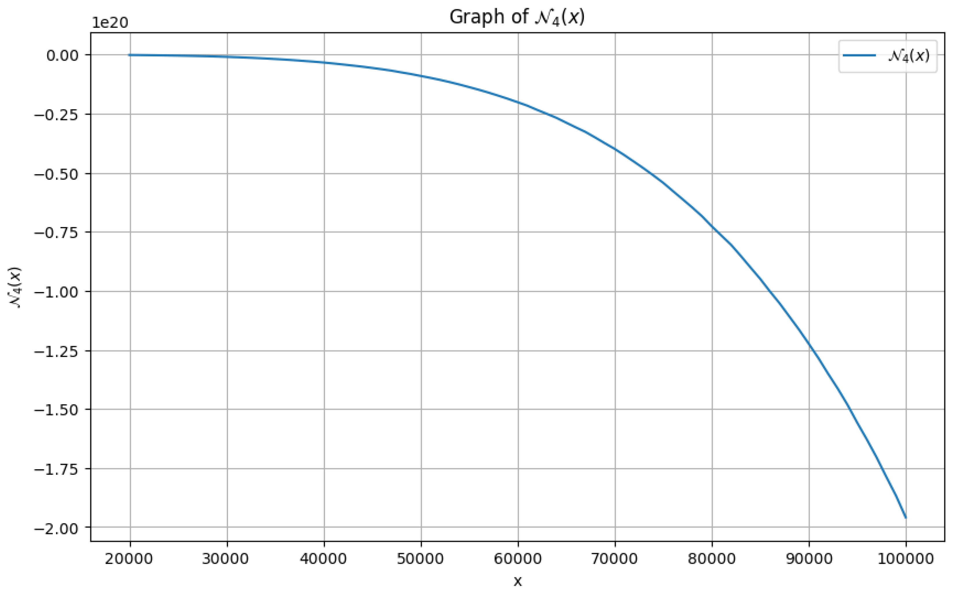
In conclusion, in both the cases, we can properly justify in this example that, (45) is definitely satisfied. Moreover, as for the sign of

N_{r} (x)

, it can be duly noted that, the main term excluding the error term is indeed negative for sufficiently large values of x. Thus, in this scenario, one can safely conclude that,

N_{r} (x) < 0

for large x.

A priori with the help of Mathematica we can indeed study the plot of

N_{3} (x)

(

m = 1, r = 3

) and

N_{4} (x)

(

m = 2, r = 4

) as compared to x for the odd and even cases respectively. (N.B. These two are some special cases for chosen values of m, one can study the same if interested using any different values of m) Subsequently, Figures and represents the respective graphs for

2 \times 10^{4} \leq x \leq 10^{5}

and considering

n = 5

Figure 5.

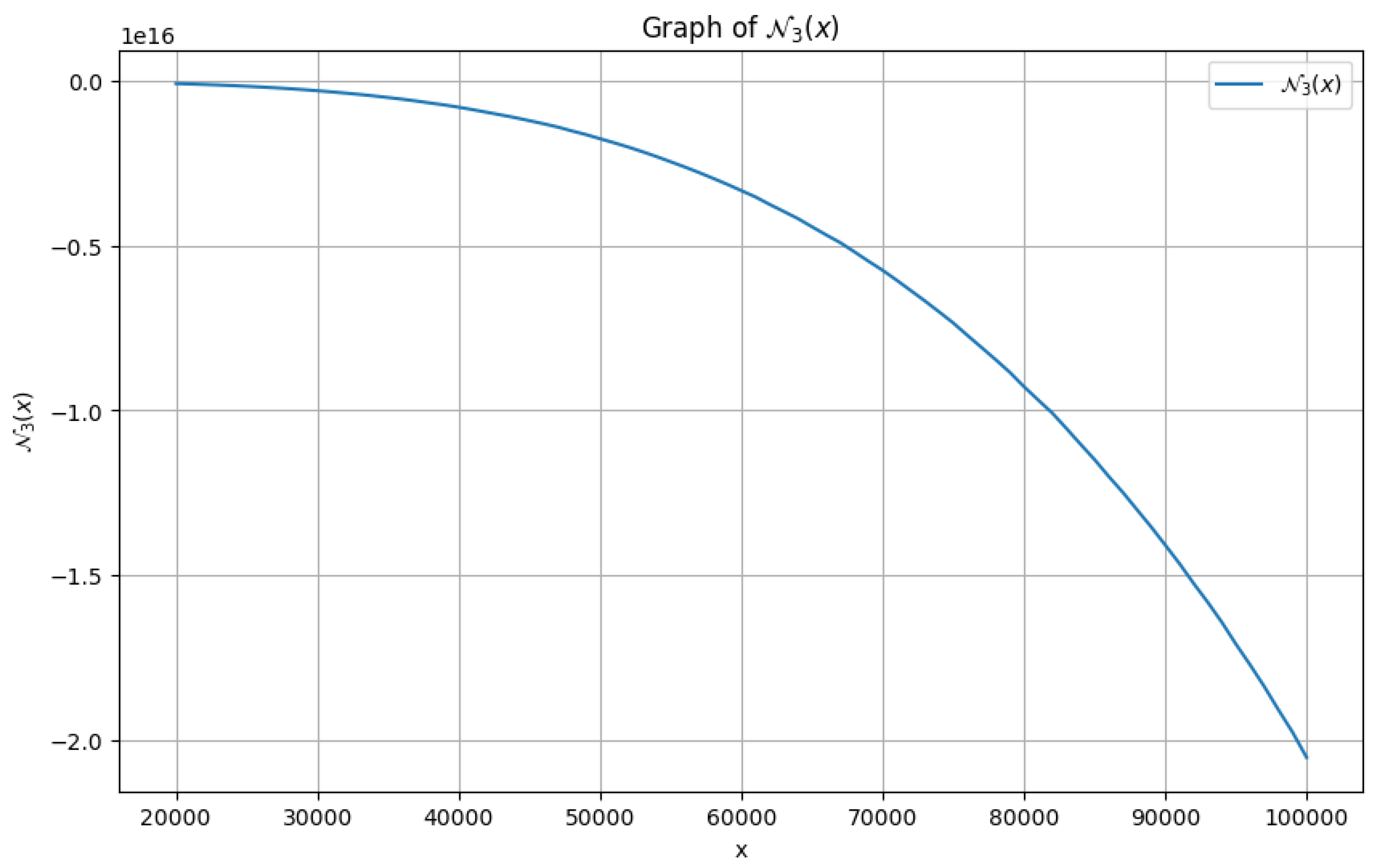
Figure 6.

Furthermore, it can be inferred from Table 5 and Table 6 that,

N_{3} (x)

and

N_{4} (x)

are strictly monotone decreasing while x assumes values in the range,

10^{4} \leq x \leq 10^{15}

. As a result, it can surely be concluded that,

N_{r} (x) < 0

for sufficiently large x, and for this particular example, i.e. for this particular choice of P, Q and R.

4.2. Furture Scope for Research

As evident from the title of the section, the above is a particular example in support of our claim (45) for the polynomial functions of the form

N (x)

as defined in (44), which heavily depends upon polynomials P, Q and R, and their respective degrees.

We can try and verify the validity of (45) by choosing P and Q and also R differently. Moreover, in this case, we have assumed the degrees of P, Q and R to be equal. Another example can be considered by varying the degrees of P and Q, and accordingly choosing degree of R accordingly. Subsequently, the order of the error term will vary.

In either case, it is very much possible that, the sign of

N (x)

shall always be negative for sufficiently large values of x, irrespective of the choice of P, Q and R, although the lower threshold for such values of x may differ.

5. Application: Equivalence with Ramanujan’s Inequality

The inequalities derived in Section 3 does have extensive applications in studying and verifying several unproven results and conjectures involving the Prime Counting Function

π (x)

. One such application which we shall observe in this section is the equivalence of the statements of the Cubic Polynomial Inequality (cf. Theorem (3.1.1)) and the Ramanujan’s Inequality (cf. Theorem (1.0.1)).

Assume that,

\begin{matrix} G (x) : = {(π (x))}^{2} - \frac{e x}{log x} π (\frac{x}{e}) \end{matrix}

(57)

Hence, the statement goes as follows.

Theorem 5.0.1.

The Cubic Polynomial Inequality isequivalentto proving the Ramanujan’s Inequality [2][3]. In other words, if

H (x) < 0

for large x, then,

G (x) < 0

for sufficiently large x and vice versa.

Proof.

A priori from (3) of Theorem (2.0.2), we attain the derivations (6) and (7).

First, we approximate

H (x)

\begin{matrix} H (x) = {(\frac{ψ (x)}{log x})}^{3} - \frac{3 e x}{log x} {(\frac{ψ (x / e)}{log x - 1})}^{2} + \frac{3 e^{2} x}{{(log x)}^{2}} (\frac{ψ (x / e^{2})}{log x - 2}) \end{matrix}

Ignoring higher-order error terms. Estimating

G (x)

in similar manner, we obtain,

\begin{matrix} G (x) = \frac{{(ψ (x))}^{2}}{{(log x)}^{2}} - \frac{e x}{log x} \frac{ψ (x / e)}{log x - 1} \end{matrix}

First we assume , if possible that,

H (x) < 0

for sufficiently large values of x. Given that

\frac{ψ (x)}{log x}

is the dominant term, for large x, thus the second term in the expression of

H (x)

will dominate the first and third terms due to the

e x

factor in the numerator. Hence, to maintain the inequality, we must have,

\begin{matrix} \frac{{(ψ (x))}^{3}}{{(log x)}^{3}} \approx \frac{3 e x}{log x} \frac{{(ψ (x / e))}^{2}}{{(log x - 1)}^{2}} \end{matrix}

Implying,

\begin{matrix} {(ψ (x))}^{3} \approx 3 e x {(ψ (x / e))}^{2} (log x) {(log x - 1)}^{2} \end{matrix}

(58)

Dividing both sides by

{(ψ (x))}^{2}

\begin{matrix} ψ (x) \approx 3 e x (log x) {(log x - 1)}^{2} \end{matrix}

N.B. Since

ψ (x)

is much larger than

ψ (x / e)

for large x, this approximation holds.

As for

G (x)

, again, given the dominance of

ψ (x)

\begin{matrix} \frac{{(ψ (x))}^{2}}{{(log x)}^{2}} \approx \frac{e x}{log x} \frac{ψ (x / e)}{log x - 1} \end{matrix}

(59)

Observe that, the leading term in

G (x)

is negative, implying

G (x) < 0

Conversely, consider that,

G (x) < 0

. This implies,

\begin{matrix} {(\frac{ψ (x)}{log x})}^{2} < \frac{e x}{log x} (\frac{ψ (x / e)}{log x - 1}) \end{matrix}

(60)

Dividing both sides by

(\frac{ψ (x / e)}{log x - 1})

, we get,

\begin{matrix} \frac{ψ (x)}{log x} < \frac{e x (ψ (x / e))}{(log x - 1)} \end{matrix}

Evaluate

H (x)

\begin{matrix} H (x) : = {(\frac{ψ (x)}{log x})}^{3} - \frac{3 e x}{log x} (\frac{{(ψ (x / e))}^{2}}{{(log x - 1)}^{2}}) + \frac{3 e^{2} x}{{(log x)}^{2}} (\frac{ψ (x / e^{2})}{log x - 2}) \end{matrix}

Given the dominance of

ψ (x)

, we can assert that,

\begin{matrix} {(\frac{ψ (x)}{log x})}^{3} < \frac{3 e x}{log x} (\frac{{(ψ (x / e))}^{2}}{{(log x - 1)}^{2}}) \end{matrix}

(61)

Which simplifies to,

\begin{matrix} {(\frac{ψ (x)}{log x})}^{3} \approx \frac{3 e x {(ψ (x / e))}^{2}}{{(log x - 1)}^{2}} \end{matrix}

(62)

Dividing both sides by

(\frac{ψ (x)}{log x})

\begin{matrix} {(\frac{ψ (x)}{log x})}^{2} \approx 3 e x (ψ (x / e)) (log x) (log x - 1) \end{matrix}

(63)

The dominant term in (63) indicates that the inequality

H (x) < 0

holds true for large enough x. This completes the proof.

□

Data Availability Statement

I as the sole author of this article confirm that the data supporting the findings of this study are available within the article [and/or] its supplementary materials.

Acknowledgments

I’ll always be grateful to Prof. Adrian W. Dudek ( Adjunct Associate Professor, Department of Mathematics and Physics, University of Queensland, Australia ) for inspiring me to work on this problem and pursue research in this topic. His leading publications in this area helped me immensely in detailed understanding of the essential concepts.

Conflicts of Interest

I as the author of this article declare no conflicts of interest.

References

Berndt, Bruce C., Ramanujan’s Notebooks: Part I, Springer New York, NY, 1985. [CrossRef]
Ramanujan Aiyangar, Srinivasa, and Bruce C Berndt, Ramanujan’s Notebooks: Part IV, New York: Springer-Verlag, 1994. [CrossRef]
Adrian, W. Dudek, David J. Platt, On Solving a Curious Inequality of Ramanujan, Experimental Mathematics, 2015; 24, 289–294. [Google Scholar] [CrossRef]
E. C. Titchmarsh, The Theory of the Riemann Zeta-function, Oxford University Press, 1951. Second edition revised by D. R. Heath-Brown, published by Oxford University Press, 1986. [CrossRef]
De, Subham. On proving an Inequality of Ramanujan using Explicit Order Estimates of the Mertens Function, Preprints 2024. [CrossRef]
L. Schoenfeld, Sharper bounds for the Chebyshev Functions θ(x) and ψ(x). II, Mathematics of Computation, vol. 30, no. 134, pp. 337-360. [CrossRef]
A. E. Ingham, The distribution of prime numbers, Cambridge University Press, 1932. Reprinted by Stechert-Hafner, 1964, and (with a foreword by R. C. Vaughan) by Cambridge University Press, 1990. [CrossRef]
F. Dress, M. F. Dress, M. El Marraki, Fonction sommatoire de la fonction de Mobius. 2, Majorations asymptotiques elementaires, Exp. Math. 2 (1993) 99-112. [CrossRef]
E. Landau, Handbuch der Lehre von der Verteilung der Primzahlen, Vol. 2 (of 2), Teubner, 1909. Reprinted by Chelsea, 1953. [CrossRef]
T. M. Apostol, Introduction to Analytic Number Theory, Springer, 1976. [CrossRef]
Jameson, G.J.O. The Prime Number Theorem, Cambridge; Cambridge University Press, London Mathematical Society student texts: Cambridge ; New York, 2003; Vol. 53. [Google Scholar] [CrossRef]
Olver, F. W. J. , Asymptotics and Special Functions, Academic Press, New York, 1974. [CrossRef]
De, Subham, On the proof of the Prime Number Theorem using Order Estimates for the Chebyshev Theta Function, International Journal of Science and Research (IJSR), Vol. 12 Issue 11, Nov. 2023, pp. 1677-1691.
L Ahlfors, Complex Analysis, McGraw-Hill Education, 3rd edition, Jan. 1, 1979. [CrossRef]
Mehdi Hassani, “On an Inequality of Ramanujan Concerning the Prime Counting Function”, Ramanujan Journal 28 (2012), 435–442. [CrossRef]
Ramanujan, S, “Collected Papers”, Chelsea, New York, 1962.
Hardy, G. H. A formula of Ramanujan in the theory of primes1. 1. London Math. Soc. 1937, 12, 94–98. [Google Scholar] [CrossRef]
Hardy, G. H. , Collected Papers, vol. II, Clarendon Press, Oxford, 1967.
Axler, Christian. On Ramanujan’s prime counting inequality. arXiv 2022, arXiv:2207.02486. [Google Scholar]
M. J. Mossinghoff, T. S. M. J. Mossinghoff, T. S. Nonnegative Trigonometric Polynomials and a Zero-Free Region for the Riemann Zeta-Function 2014, arXiv:1410.3926. [Google Scholar]
T. S. Trudgian, Updating the Error Term in the Prime Number Theorem, Ramanujan J., 2014.
T. Oliveira e Silva, Tables ofValues of π(x) and π2(x), Available online: http://www.ieeta.pt/∼tos/primes.html, 2012.

Table 1. Values of

H (x)

for

10^{4} \leq x \leq 10^{18}

Table 1. Values of

H (x)

for

10^{4} \leq x \leq 10^{18}

$x = 10^{k}$	$H (x)$
$10^{4}$	$- 4.822952515086 \times 10^{8}$
$10^{5}$	$- 1.9535582364473376 \times 10^{11}$
$10^{6}$	$- 9.742665854621681 \times 10^{13}$
$10^{7}$	$- 5.373324095991878 \times 10^{16}$
$10^{8}$	$- 3.2776888213143585 \times 10^{19}$
$10^{9}$	$- 2.142500053569382 \times 10^{22}$
$10^{10}$	$- 1.4738226482632569 \times 10^{25}$
$10^{11}$	$- 1.0555737602257731 \times 10^{28}$
$10^{12}$	$- 7.810947114144009 \times 10^{30}$
$10^{13}$	$- 5.937547995444999 \times 10^{33}$
$10^{14}$	$- 4.6163278697477706 \times 10^{36}$
$10^{15}$	$- 3.65847701300371 \times 10^{39}$
$10^{16}$	$- 2.947501336471066 \times 10^{42}$
$10^{17}$	$- 2.4089115035201524 \times 10^{45}$
$10^{18}$	$- 1.9935903086211532 \times 10^{48}$

Table 2. Values of

K (x)

for

10^{4} \leq x \leq 10^{17}

Table 2. Values of

K (x)

for

10^{4} \leq x \leq 10^{17}

$x = 10^{k}$	$K (x)$
$10^{4}$	$6.785501979995337 \times 10^{11}$
$10^{5}$	$2.858713229490609 \times 10^{15}$
$10^{6}$	$1.3657430631495643 \times 10^{19}$
$10^{7}$	$7.37684110441765 \times 10^{22}$
$10^{8}$	$4.2993020901898284 \times 10^{26}$
$10^{9}$	$2.6664968326322003 \times 10^{30}$
$10^{10}$	$1.7394264262779463 \times 10^{34}$
$10^{11}$	$1.1821189632007215 \times 10^{38}$
$10^{12}$	$8.310509439561298 \times 10^{41}$
$10^{13}$	$6.010924984361412 \times 10^{45}$
$10^{14}$	$4.454174125769207 \times 10^{49}$
$10^{15}$	$3.3701437003780375 \times 10^{53}$
$10^{16}$	$2.59663004179433 \times 10^{57}$
$10^{17}$	$2.0327843159078997 \times 10^{61}$

Table 3. Values of

L (x)

for

10^{4} \leq x \leq 10^{16}

Table 3. Values of

L (x)

for

10^{4} \leq x \leq 10^{16}

$x = 10^{m}$	$L (x)$
$10^{4}$	$5.442878634267854 \times 10^{6}$
$10^{5}$	$3.182941989056241 \times 10^{8}$
$10^{6}$	$2.0720876553125698 \times 10^{10}$
$10^{7}$	$1.453173495473891 \times 10^{12}$
$10^{8}$	$1.0748621057424523 \times 10^{14}$
$10^{9}$	$8.271311872938837 \times 10^{15}$
$10^{10}$	$6.562072688654034 \times 10^{17}$
$10^{11}$	$5.3333332449648206 \times 10^{19}$
$10^{12}$	$4.4203146604764075 \times 10^{21}$
$10^{13}$	$3.723359062321086 \times 10^{23}$
$10^{14}$	$3.1792547132494815 \times 10^{25}$
$10^{15}$	$2.7463355733587377 \times 10^{27}$
$10^{16}$	$2.3962303815115464 \times 10^{29}$

Table 4. Values of

F (x)

for

10^{4} \leq x \leq 10^{14}

Table 4. Values of

F (x)

for

10^{4} \leq x \leq 10^{14}

$x = 10^{m}$	$F (x)$
$10^{4}$	$- 377, 275.13516957406$
$10^{5}$	$- 1.830179494511997 \times 10^{7}$
$10^{6}$	$- 1.0203946684413686 \times 10^{9}$
$10^{7}$	$- 6.256701329540303 \times 10^{10}$
$10^{8}$	$- 4.1109224248432134 \times 10^{12}$
$10^{9}$	$- 2.8451189547136775 \times 10^{14}$
$10^{10}$	$- 2.0504855777527976 \times 10^{16}$
$10^{11}$	$- 1.5264989872331325 \times 10^{18}$
$10^{12}$	$- 1.1670093161419563 \times 10^{20}$
$10^{13}$	$- 9.121682100604639 \times 10^{21}$
$10^{14}$	$- 7.264828101112622 \times 10^{23}$

Table 5. Values of

N_{3} (x)

for

10^{4} \leq x \leq 10^{15}

Table 5. Values of

N_{3} (x)

for

10^{4} \leq x \leq 10^{15}

$x = 10^{m}$	$N_{3} (x)$
$10^{4}$	$- 6.204817261289663 \times 10^{12}$
$10^{5}$	$- 2.0538877597403304 \times 10^{16}$
$10^{6}$	$- 8.54030555139954 \times 10^{19}$
$10^{7}$	$- 4.1469160311751975 \times 10^{23}$
$10^{8}$	$- 2.2502470326411468 \times 10^{27}$
$10^{9}$	$- 1.3249101964920937 \times 10^{31}$
$10^{10}$	$- 8.304086276172884 \times 10^{34}$
$10^{11}$	$- 5.4674077933205056 \times 10^{38}$
$10^{12}$	$- 3.746002497341975 \times 10^{42}$
$10^{13}$	$- 2.6523089311884873 \times 10^{46}$
$10^{14}$	$- 1.930438588096488 \times 10^{50}$
$10^{15}$	$- 1.4384149341267808 \times 10^{54}$

Table 6. Values of

N_{4} (x)

for

10^{4} \leq x \leq 10^{15}

Table 6. Values of

N_{4} (x)

for

10^{4} \leq x \leq 10^{15}

$x = 10^{m}$	$N_{4} (x)$
$10^{4}$	$- 7.911694463952808 \times 10^{15}$
$10^{5}$	$- 1.9593096354084415 \times 10^{20}$
$10^{6}$	$- 6.465704751724349 \times 10^{24}$
$10^{7}$	$- 2.597975844704281 \times 10^{29}$
$10^{8}$	$- 1.2022000181431568 \times 10^{34}$
$10^{9}$	$- 6.170254706864245 \times 10^{38}$
$10^{10}$	$- 3.427910948552053 \times 10^{43}$
$10^{11}$	$- 2.026811001937711 \times 10^{48}$
$10^{12}$	$- 1.260254434482889 \times 10^{53}$
$10^{13}$	$- 8.168086531604906 \times 10^{57}$
$10^{14}$	$- 5.481394602239431 \times 10^{62}$
$10^{15}$	$- 3.7889284123142535 \times 10^{67}$

Disclaimer/Publisher’s Note: The statements, opinions and data contained in all publications are solely those of the individual author(s) and contributor(s) and not of MDPI and/or the editor(s). MDPI and/or the editor(s) disclaim responsibility for any injury to people or property resulting from any ideas, methods, instructions or products referred to in the content.

© 2024 by the authors. Licensee MDPI, Basel, Switzerland. This article is an open access article distributed under the terms and conditions of the Creative Commons Attribution (CC BY) license (http://creativecommons.org/licenses/by/4.0/).

Copyright: This open access article is published under a Creative Commons CC BY 4.0 license, which permit the free download, distribution, and reuse, provided that the author and preprint are cited in any reuse.

Downloads

353

Views

170

Comments

Subscription

Notify me about updates to this article or when a peer-reviewed version is published.

MDPI Initiatives

Important Links

Choose an area of interest and we will send you notifications of new preprints at your preferred frequency.

Disclaimer

Studying some Inequalities involving Polynomial Functions in π(x)

Abstract

Keywords:

Subject:

1. Introduction and Motivation

2. Important Derivations Regarding π ( x )

3. Inequalities Involving Polynomials in π ( x )

3.1. Cubic Polynomial Inequality

3.2. Higher-Degree Polynomial Inequality

3.3. Quadratic Form Involving Sums of Prime Counting Function

3.4. Logarithmic Weighted Sum Inequality

4. A More General Framework

4.1. A Typical Example

4.1.1. deg(P), deg(Q) and deg(R) Are Odd

4.1.2. deg(P), deg(Q) and deg(R) Are Even

4.2. Furture Scope for Research

5. Application: Equivalence with Ramanujan’s Inequality

Data Availability Statement

Acknowledgments

Conflicts of Interest

References

MDPI Initiatives

Important Links

Subscribe

2. Important Derivations Regarding $π (x)$

3. Inequalities Involving Polynomials in $π (x)$