Submitted:
28 June 2024
Posted:
01 July 2024
You are already at the latest version
Abstract
Keywords: domain adversarial; channel reconstruction; transfer learning; fault diagnosis
Keywords:
bearing fault diagnosis
1. Introduction
High-speed trains (HST) are often considered one of the best modes of transportation, and the maximum operating speed of HST can reach up to 380 km/h [1]. At such high speeds, bearings, as important parts in the transmission system, are subjected to complex alternating loads, which increase the wear rate of the bearings and reduce their service life [2]. As an important part of the HST, whose health situation is greatly related to the operation of the whole train.
Majority of the existing research on bearing fault diagnosis is primarily targeted at the vibration signals generated by bearing impacts, which contain information concerning the healthy situation of the bearings, and the analysis of the vibration signals and the information concerning the healthy situation of the bearings is crucial to the diagnosis of bearing faults in high-speed trains. With the proposition of machine learning methods, more and more academics have studied the correlated intelligent diagnosis algorithms and have successfully produced a variety of effective fault diagnosis algorithms on the basis of vibration acceleration signals. Conventional intelligent diagnostic approaches have often used a mixture of signal processing measures and classification methods, using signal processing measures that have a well-established theoretical foundation, such as variational modal decomposition (VMD) [3], empirical modal decomposition (EMD) [4], and empirical wavelet transform (EWT) [5], to obtain signal features. These features are then input into classification methods such as support vector machines (SVMs), extreme learning machines (ELM) [6], and back-propagation networks (BPNN) [7] to recognize the bearing fault state. Although these methods can classify and identify the bearing fault state, the accuracy of its diagnosis is strongly linked to the fault features extracted by the conventional signal processing methods in the previous period. Feature extraction using traditional signal processing methods mainly relies on personal experience, it is difficult to sufficiently extract the correlated information in the vibration signal. This results in low-quality feature extraction, thus affecting the accuracy of the final fault identification.
Zhang et al. [8] combined the spatial discard regularization method with separated convolution to extract features from the original signals, achieving effective differentiation of the original signals of bearings in different states. Liu et al. [9] used improved one-dimensional and two-dimensional convolutional neural networks to achieve intelligent recognition of bearing states, demonstrating high recognition accuracy. Che et al. [10] combined a deep belief network and convolutional neural network to extract relevant information from grayscale images and time series signals, and the fault types are recognized using the deep learning model fused into it. More adaptable intelligent fault diagnosis approaches based on deep learning [11,12,13] can be used to feature the vibration data automatically. However, its excellent performance depends on massive amounts of well-labeled training data and requires that the training data and the test data fulfill the condition of being identically distributed. In practical engineering work, owing to the effects of the complex working environment, it is difficult to obtain plenty of data with markers which are of the same distribution, leading to the fact that all kinds of intelligent fault diagnosis measures on the basis of deep learning can't be applied effectively.
In an intelligent fault diagnosis approach that is based on migration learning, the data for model training and testing do not need to have the same probability distribution. This can be accomplished by exploiting the source domain with the help of technical methods of migration to accomplish the tasks in the target domain, especially for data samples where there are no or few markers in the target domain [14]. Currently, on the basis of various deep neural networks, more and more scholars have proposed several migration learning methods for rotating machinery fault diagnosis, and experimental validation has been carried out on various types of datasets collected under different operating conditions [15,16]. Domain adaptation is one of the migration learning methods and can be used to automatically alignment of feature distributions in the source and target domains for deep feature extraction by using distribution difference metric functions such as maximum mean difference (MMD), multinomial kernel maximum mean difference (MK-MMD), and Wassertein distance, which in turn realizes the migration from the source domain to the target domain to accomplish the task demands on the target domain. Li et al. [17] added the multiple maximum mean difference (MK-MMD) to the deep transfer network model to reduce the distributional difference of the data in the two domains and realize the fault identification of the target domains. Wan et al. [18] utilized the multiple kernel maximum mean discrepancy to adjust the marginal distribution and the conditional distribution in the multidomain discriminators of the two domains to achieve the extraction of domain invariable features and complete cross-domain fault identification. Guo et al. [19] embedded the maximum mean difference into a fully connected layer in a convolutional neural network, thus enabling domain invariant feature extraction to achieve pattern recognition of faults. Wen et al. [20] added an adversarial mechanism in combination with an autoencoder to achieve cross-domain diagnosis from experimental bearings to the actual wheelset bearings used in the test models. Wan et al. [21] combined an adversarial mechanism with a multiple kernel maximum mean discrepancy to achieve cross-domain diagnosis, integrating the adversarial mechanism and multiple kernel maximum mean discrepancy into a deep convolutional model to achieve cross-domain bearing fault diagnosis. Zhang et al. [22] presented an improved domain adversarial neural network with improved multi-feature fusion to achieve the classification of bearing health status. Wu et al. [23] combined the adversarial mechanism and maximum mean discrepancy with a weight-sharing convolutional neural network to achieve fault identification under different operating conditions.
In summary, there have been many researchers who have investigated deep migration learning methods in various perspectives to improve its performance for bearing fault state recognition. However, compared to conventional bearings, the forces on rolling bearings in high-speed trains are more complex and variable. Based on the conditions of variable load and existing theories, a migration model for fault diagnosis, which incorporates an adversarial mechanism and a channel reconstruction unit (CRU), is established. In the process of establishing the model, we analyze not only the influence of each module in the feature extractor on the performance of feature extraction but also the effect of the structure of the fault recognition module and domain discrimination module on the diagnosis accuracy. Finally, the method is experimentally analyzed to have good performance in identifying bearing fault states under different load conditions.
2. Basic Theory
The characterization of the data and its edge distribution are assumed to be represented by and . Thus, represents a domain. Two domains that are not the same indicate differences about characterization or edge distributions. denotes the source domain while denotes the target domain. These two domains comprise bearing vibration data under various loads with the same labels but distinct edge distributions, . The purpose of transfer learning is to aid in accomplishing tasks in the target domain by leveraging message from source domain. Domain Adversarial Neural Network (DANN) [24] stands as one of the classical methods in transfer learning.
Domain Adversarial Neural Network (DANN) mainly include a feature extractor , a domain discriminant module and a fault recognition module . The feature extractor primarily performs deep feature extraction on the input data, while the fault identification module is responsible for identifying faults on the target domain test data samples after feature extraction. The domain discriminant module serves as a binary classifier with an added gradient inversion layer.
represents input data, and the characterization extractor learn the features of the data samples by updating the parameter , which can be denoted as . The features learned by the extractor are then inputted to the fault recognition module for fault recognition, represented as . The loss function expressed as Equation (1)
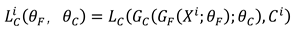
Where denotes the sample, denotes the fault category of the sample, andrepresent the parameters of the feature extractorsand the fault recognition module.The domain discrimination module is utilized to discriminate the from that domain,and its loss function is given in Equation (2).

Where represents the parameters of the domain discriminative module and denotes the label of the domain. Loss function is shown in Equation (3).
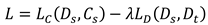
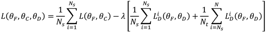
Where and denote the samples and there corresponding true labels, denotes the samples in the target domain, and is the equilibrium parameter. The total quantity of samples is assumed to be . and represent the quantity of samples in the source and target domains. The total loss function is shown in Equation (4).
3. Fault Diagnosis Transfer Model
To enable bearing fault diagnosis under different loading conditions, this paper proposes a novel transfer learning method by combining the domain adversarial neural network with the channel reconstruction unit module (CRU). Initially, the signal undergoes preprocessing, converting the original signal into a one-dimensional tensor, which is then fed into the feature extractor. Subsequently, domain invariable features are extracted through adversarial learning to facilitate modal recognition for unlabeled target domain samples. The model structure depicted in Figure 1, with further details described below.
3.1 Feature Extractor
The feature extractor comprises five feature extraction modules and five channel reconstruction modules. Each feature extraction module includes a one-dimensional convolutional layer, a normalization layer, and a maximum pooling layer, as illustrated in Figure 2. The parameters of each feature extraction module are detailed in Table 1.
The space formed by the source domain samples and the target domain samples is , is the data length for every smple. The convolution operation on the input data is expressed as Equation 5.
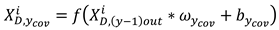
Where represents the output of the last feature extraction module, denotes the output of the current yth module, denotes the training parameters for the weights and biases in the convolutional computation, denotes the linear rectifier unit (RELU) activation function, the input to the first feature extraction module is a data sample that has undergone signal preprocessing.
Then the samples after the convolution operation are input into the normalization layer for normalization operation to prevent the order of magnitude difference of the input variables from affecting the operation results too much. The normalization operation process is shown in Equation 6.
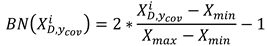
Where shows the maximum and minimum values in the operational data. Following normalization, the maximum pooling operation is applied on the normalized to reduce the model parameters and the operation cost. The maximum pooling operation is shown in Equation (7).

Where represents the length of the segment and is the starting point of the pooling position.
3.2. Basic Theory of CRU
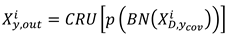
Following feature extraction by the yth feature extraction module, the output is then input to the channel reconstruction unit (CRU). The CRU, as depicted in Figure 3 was proposed by Li et al [25]. Unlike standard convolution, CRU employs splitting, transforming, and reconstruction strategies.
The first is the splitting strategy, which divides the pass into two parts, and channels, as depicted in figure 3. Here is the splitting ratio. The channels of feature mapping are subsequently compressed using convolution to improve the efficiency of computation. Following splitting, the feature channel is squeezed and the squeezing ratio is 2. Following splitting and squeezing, the feature from the feature module is divided into the upper portion and the lower portion , then enters into the transformation stage, with is inputted to the upper transformation stage. In the upper transformation stage, Group-by-Group Convolution (GWC) [26] and Point-by-Point Convolution (PWC) are used instead of convolution operation to extract deep information. The GWC and PWC operations are performed on the upper part of the output. After that, we sum the outputs to form the merged feature . The upper transform stage can be expressed by Equation 8 as:
Where , are the relevant parameters of GWC and PWC.
is input to the lower transform stage to generate features with shallow hidden details using PWC operation. This serves as a complement to the rich features generated earlier. Utilizing allows for the generation of additional features without incurring extra costs. Finally, the newly generated features and the reused features are concatenated to form the feature , and the lower transformation stage formula is shown in Equation (9):
Where is the relevant parameters of the lower input PWC.
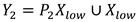
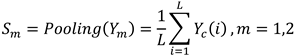
After the transformation, the output features , of the upper and lower transformation stages are fused using the simplified Sknet method [27], as depicted in the fusion section in Figure 3. Applying global average pooling to collect global spatial message for , which is computed as in Equation (10).
The global up-channel descriptions and global down-channel descriptions are then stacked together, and a channelized soft attention operation is used to generate the feature importance vectors and . Finally, the up- and down-channel descriptions are combined with by combining the upper feature and lower feature are merged by channel to obtain the channelized refinement feature . As in Equation (11) and Equation (12).
The result of the final processing of the features input from the feature module by the channel reconstruction unit can be expressed as Equation (13).
3.3. Fault Recognition Module
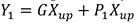
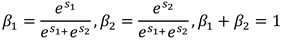
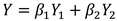
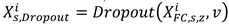
The output of the feature extractor is , which contains feature information learned from both domains. represents features learned from source domains that contain useful knowledge. The fault identification module consists of two fully connected layers, a layer and the output layer. The zth fully connected layer processes as in Equation (14).

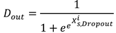
Where represents the parameters of the fully connected layer. Dropout's process for the second fully connected layer can be expressed as Equation (15).
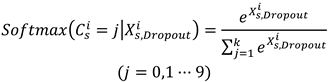
Where is the deactivation rate, which is taken as 0.5 in this paper. The softmax function is used as the output layer to identify the class of faults, the softmax function can be expressed as Equation (16)
Where denotes the fault label recognized by the output layer. The loss function of the fault recognition module is expressed as Equation (17).
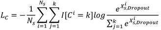
Where is the quantity of fault categories in the data sample and represents the indicator function.
3.4. Domain Discriminator Module
The structure of the domain discrimination module mirrors that of the fault recognition module, but the domain discrimination module is used to differentiate the domain labels of the samples by the features output from the feature extractor. The domain class of the sample is judged after first performing a convolution operation on the feature through two fully-connected layers as in Equation (14), then processed through a dropout layer as in Equation (15), and finally through an output layer. The output can be expressed as Equation (18).
When the output layer cannot discriminate the samples from that domain, its learned features are domain invariant features. Equation (19) is the loss function of the domain discrimination module .

where the domain label “0” or “1” and is the prediction label.
3.5.Model Loss Function
In the domain adversarial neural network adversarial training, the total loss function is expressed as Equation (20).

Where the equilibrium parameter varies dynamically with the number of iterations and the expression is shown in Equation (20).
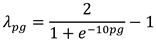
Where represents the training iteration relative process, and represents the rate of the times of current iterations to the total times of iterations.
4. Experiments
4.1. Case Western Reserve University (CWRU) Bearing Experiment Data Analysis
The CWRU's bearing dataset has been extensively utilized by researchers to validate various diagnostic methods. For the purposes of this section, the sampling frequency of the system chosen to collect the bearing vibration acceleration data is 48 kHz, the motor speed is 1797 r/min, and the load sizes applied to the bearings in the experimental conditions are 1 hp, 2 hp, and 3 hp. The bearings exhibit four health states at each load: normal condition (N), inner ring failure (IN), outer ring failure (OF), and roller failure (RF). Each failure state of the bearing includes three different damage levels in addition to the healthy state: 0.007 inches, 0.014 inches, and 0.021 inches. Two of the three different load conditions are chosen as the source domain dataset and the target domain dataset, respectively, and then 2,000 samples are randomly chosen from the sample data associated with each health state to serve as the training and testing sample sets for the two domains, and the total quantity of samples for training and testing is 40,000. The data setup under the experimental operation is summarized in Table 2, while the dataset under each load condition is presented in Table 3. Figure 4 illustrates the dataset for the 1 hp load condition under normal conditions, along with the time and frequency domain images of signals for each fault condition with a damage level of 0.007 inches.
4.1.1. Effect of Individual Modules on Experimental Test Results
In order to demonstrate the performance of this paper's kind of fault diagnostic model, the test results of methods lacking adversarial mechanisms or channel reconstruction units and this paper's method are visualized using the t-distributed stochastic neighbor embedding(t-SNE) algorithm. The visualization results of the migration task from Domain B to Domain A are depicted in Figure 5. In each category, there is a notable distribution of samples. However, as shown in Figure 5(a), when the adversarial mechanism is absent, a more severe cross-mixing phenomenon occurs between categories due to differences in data distribution. The model that lacks the adversarial mechanism is poor for recognizing the test samples in the target domain. In Figure 5(b), each category of samples has a large distance between them, and confounding occurs between sample class 7 and sample class 0. However, when deep features are extracted using the paper’s method, the method is better able to aggregate samples in each health state compared to the previous two methods.
As illustrated in confusion matrix in Figure 6, it can be seen that due to the lack of an adversarial mechanism, the accuracy of each category shown in Figure 6(a) is relatively low, especially for category 4, which has an accuracy of only 45%. (b) and Figure 6(c) depict that the adversarial module can effectively extract consistent features from the two domains and improve the accuracy of bearing fault recognition. Additionally, comparing Figure 6(b) and 6(c), the accuracy of nearly every category reaches 100% after introducing the channel reconstruction unit in the feature extractor. This indicates that deeper features associated with faults can be effectively learned after the introduction of the channel unit, reflecting the model's superiority. The results of other migration tasks for the three methods are shown in Table 4.
4.1.2. Impact of FC Layers on Experimental Test Results
Throughout the model, besides the feature extractor, the performance of the algorithm is also affected by the parameters in the fault identification module and the domain discrimination module. To investigate the effect of fully connected layers on the algorithm's performance, experiments were conducted to assess the classification accuracy with different quantity of fully connected layers over a certain number of iterations. According to the results in Table 5, it was found that the classification accuracy was higher in the structure that used two fully connected (FC) layers, a dropout layer, and an output layer. This is because a lower number of fully connected layers in the classifier reduces the model's expressive ability, adversely affecting its performance and failing to achieve the desired classification effect. On the other hand, a higher number of layers increases the model's computational cost and can easily lead to overfitting, negatively impacting the classifier's effectiveness. Based on this, the fault recognition module and domain discrimination module are structured with two fully connected layers, a dropout layer, and an output layer.
4.1.3. Comparative Experimental Analysis with Other Methods
The proposed method in this paper is analyzed on the Case Western Reserve University bearing dataset as shown in Table 6, where the number of samples per run condition is 40,000 and there are 2000 training samples and 2000 test samples included in each state. This paper's module is also compared with three other methods, which are SDAE+JGSA [28], DDC [29], and DACNN [30]. With the SDAE+JGSA method there are 3000 samples for each operating condition and every health state contains 300 samples. The algorithm first extracts the deep features of the image using the SDAE algorithm and then reduces the feature distribution differences using the JGSA algorithm.
As the results in Table 6 show, the first two methods utilize SAE and CNN to join the relevant JGSA and domain confusion loss function to align the distribution differences, and the highest diagnostic accuracy can be up to 98.3%, and both DACNN and the present method introduce the adversarial mechanism and thus realize the extraction of domain-invariant features; however, compared with DACNN, the present paper effectively improves the model to extract deeper features, as expressed from the table, each task of this paper's method has a better performance than the DACNN method, which shows that the introduction of CRU in domain adversarial network has a significant effect in increasing the diagnostic performance of bearing faults.
4.2. Analysis of Experimental Data of Bearing Failure Simulation on Bearing Life Prediction Test Bench
In the previous section of CWRU, the bearing data sets A, B, and C have loads corresponding to 1hp, 2hp, and 3hp, at a speed of 1797 rpm. the above experiments simulate the application performance for models with various load at the same speed, and for the purpose of further test the generalization performance of the models, the same simulation conditions are used in this section, and the four data samples are selected for experimental validation of the model.
4.2.1. LY-GZ-02 Experimental Bench Data Description
Select bearing model LZ-GZ-02 bearing experimental bench to simulate the faulty bearing working condition under normal working conditions, and use vibration acceleration sensors and data acquisition devices to collect vibration data under each faulty condition of the bearing. Figure 7 illustrates the relevant parts of the experimental setup, which mainly consists of hydraulic cylinders, operating table, data collector and other devices.
Four different states of health under the bearing respectively at the same speed of three different load conditions of operation. The bearing health states include normal (N), outer ring fault (OF), inner ring fault (IF) and rolling element fault (RF). As shown in Table 7, the loads are 0 N, 1000 N and 2000 N. The sampling frequency of the experimental acquisition device is 20 KHz. For each type of load, the samples for each bearing state are 1000, and the sample length is 1024. The time frequency images of the vibration acceleration signals of the bearings at 1000 rpm with the loads of 1000N for the four states are shown in Figure 8.
4.2.2. Experimental Comparisons
TCA, JDA and DACNN are validated with the performance of the proposed method presented herein. TCA utilizes kernel functions to map the number of samples into a high-dimensional regenerative kernel Hibert space, which narrows down the differences in the distribution of the pre-existing data and preserves the domain invariable features. In TCA, the radial basis function is chosen as the kernel function of TCA.JDA (Joint Distribution Adaptation) is traditional transfer learning methods, which extracts domain invariable features and predicts the target domain by maximizing the difference in the distribution of the categories of the source and target domains for the mapping of each category. In JDA, radial basis functions are selected. DACNN is also a migration learning model that learns domain invariant features using CNN and with adversarial mechanisms.
As can be illustrated in Table 8, the diagnostic accuracies of the TCA method and the JDA method between the three load conditions are 76.1% and 75.4%, respectively, which indicates that pure kernel space mapping and two domain categories The spatial mapping between them is hard to obtain valuable features under various loading conditions. Compared to the present method DACNN method fails to regard the significance and uniqueness of the features of the recognition process in the feature learning process, and the recognition accuracy is lower. This method further extracts the deep features in the samples by adding the channel reconstruction unit to the feature extractor species, and accordingly, the accuracy of the test between condition B and condition C reaches 100%, and the mean accuracy of the three conditions is 99.4%, which is clearly better than that of other methods.
A and B for the results shown in Figure 9 are the source and target domains, respectively. As depicted in Figure 9(a) and Figure 9(b), the feature categories learned by the TCA and JDA methods do not really perform effective alignment of distributional differences, and there are most of the samples labeled 3 (outer-ring faults) are incorrectly predicted, which do not allow for effective feature identification and sample classification. While the method shown in Figure 9(c) has improved in the overall effect, the adversarial training in a certain sense makes the network effectively learn the domain invariable features, which positively affects the fault classification module in the prediction of the test samples, but compared this paper’s model, this model has better capability of feature learning compared to DACNN, which can more obviously recognize the various health states of the target domain bearings. The results of the above analysis show that this model is superior to the other three models, and the combination of the adversarial mechanism and the channel reconstruction unit can significantly improve the fault diagnosis performance of the bearings under different loading conditions.
5. Conclusions
In this paper, a migration learning model combining domain adversarial network and CRU is proposed for high-speed train bearing fault diagnosis under variable load conditions. The model has three advantages: Firstly, the normalization is added to the feature extraction module to reduce the influence of individual difference samples on the network model, and the RELU activation function is used to improve the speed of the model operation. Secondly the influence of each module in the feature extractor on the performance of the algorithm is analyzed through experiments, and it is finally determined that the feature extraction module is combined with the CRU to strengthen the model's ability to learn domain invariant features. Finally, experimentally analyzing the impact of the quantity of fully connected layers on the performance of the algorithm, it is determined that the structure of the fault identification module and the domain discrimination module consists of two fully connected layers combined with the Dropout function, which reduces the model parameters and reduces the risk of model overfitting. In addition to this, the present method is compared with existing intelligent diagnosis methods to verify the good performance of the present method. However, this method only investigates the fault diagnosis under different load conditions in the same equipment, so in the next study, we will investigate the migration fault diagnosis method in different machines and equipment of high-speed trains or different types of bearings in the same equipment, so as to better monitor the health status of high-speed train bearings.
Author Contributions
Conceptualization, Y.Z. and W.Z.; methodology, W.Z.; software, W.Z.; validation, W.Z., T.L. and X.Z.; data curation, W.Z., T.L. and X.Z; writing—original draft preparation, W.Z.; writing—review and editing, Y.Z. and Y.S.; visualization, W.Z.; supervision, Y.S.; All authors have read and agreed to the published version of the manuscript.
Funding
This research was funded by Jilin Provincial Department of Science and Technology, Grant number 20230101208JC.
Institutional Review Board Statement
Not applicable.
Informed Consent Statement
Not applicable.
Data Availability Statement
The dataset used in Experiment 1 of this paper can be found at the following link: https://engineering.case.edu/bearingdatacenter/welcome. Data from Experiment 2 in this study are available upon request from the corresponding author. For privacy reasons, these data are not publicly available.
Conflicts of Interest
The authors declare no conflicts of interest.
References
- W. Hu, G. Xin, J. Wu, G. An, Y. Li, K. Feng, and J. Antoni, "Vibration-based bearing fault diagnosis of high-speed trains: A literature review," High-speed Railway, vol. 1, no. 4, pp. 219-223, Dec. 2023. [CrossRef]
- D. Hou, H. Qi, D. Li, C. Wang, D. Han, H. Luo, and C. Peng, "High-speed train wheel set bearing fault diagnosis and prognostics: Research on acoustic emission detection mechanism," Mechanical Systems and Signal Processing, vol. 179, Nov. 2022, Art. no. 109325. [CrossRef]
- K. Dragomiretskiy and D. Zosso, ‘‘Variational mode decomposition,’’ IEEE Trans. Signal Process., vol. 62, no. 3, pp. 531–544, Nov. 2014.
- J. B. Ali, N. Fnaiech, L. Saidi, B. Chebel-Morello, and F. Fnaiech, ‘‘Application of empirical mode decomposition and artificial neural network for automatic bearing fault diagnosis based on vibration signals,’’ Appl. Acoust., vol. 89, pp. 16–27, Mar. 2015. [CrossRef]
- Q. Zhang, J. Ding, and W. Zhao, ‘‘An adaptive boundary determination method for empirical wavelet transform and its application in wheelset-bearing fault detection in high-speed trains,’’ Measurement, vol. 171, Feb. 2021, Art. no. 108746. [CrossRef]
- C. He, T. Wu, R. Gu, Z. Jin, R. Ma, and H. Qu, ‘‘Rolling bearing fault diagnosis based on composite multiscale permutation entropy and reverse cognitive fruit fly optimization algorithm – Extreme learning machine,’’ Measurement, vol. 173, Mar. 2021, Art. no. 108636. [CrossRef]
- J. Li, X. Yao, X. Wang, Q. Yu, and Y. Zhang, ‘‘Multiscale local features learning based on BP neural network for rolling bearing intelligent fault diagnosis,’’ Measurement, vol. 153, Mar. 2020, Art. no. 107419. [CrossRef]
- J. Zhang, X. Kong, X. Li, Z. Hu, L. Cheng, and M. Yu, ‘‘Fault diagnosis of bearings based on deep separable convolutional neural network and spatial dropout,’’ Chin. J. Aeronaut., vol. 35, no. 10, pp. 301–312, Oct. 2022. [CrossRef]
- X. Liu, W. Sun, H. Li, Z. Hussain, and A. Liu, ‘‘The method of rolling bearing fault diagnosis based on multi-domain supervised learning of convolution neural network,’’ Energies, vol. 15, no. 4614, Apr. 2022. [CrossRef]
- C. Che, H. Wang, X. Ni, and R. Lin, ‘‘Hybrid multimodal fusion with deep learning for rolling bearing fault diagnosis,’’ Measurement, vol. 173, Mar. 2021, Art. no. 108655. [CrossRef]
- Z. Zhu, Y. Lei, G. Qi, Y. Chai, N. Mazur, Y. An, and X. Huang, ‘‘A review of the application of deep learning in intelligent fault diagnosis of rotating machinery,’’ Measurement, vol. 206, Jan. 2023, Art. no. 112346. [CrossRef]
- S. Zhang, S. Zhang, B. Wang, and T. G. Habetler, ‘‘Deep learning algorithms for bearing fault diagnostics—A comprehensive review,’’ IEEE Access, vol. 8, pp. 29857–29881, Feb. 2020.
- S. R. Saufi, Z. A. B. Ahmad, M. S. Leong, and M. H. Lim, ‘‘Challenges and opportunities of deep learning models for machinery fault detection and diagnosis: A review,’’ IEEE Access, vol. 7, pp. 122644–122662, Aug. 2019. [CrossRef]
- S. Pan and Q. Yang, ‘‘A survey on transfer learning,’’ IEEE Trans. Knowl. Data Eng., vol. 22, no. 10, pp. 1345–1359, Oct. 2010. [CrossRef]
- L. Misbah, C. K. M. Lee, and K. L. Keung, ‘‘Fault diagnosis in rotating machines based on transfer learning: Literature review,’’ Knowl.-Based Syst., vol. 283, Jan. 2024, Art. no. 111158. [CrossRef]
- M. Hakim, A. A. B. Omran, A. N. Ahmed, M. Al-Waily, and A. Abdellatif, ‘‘A systematic review of rolling bearing fault diagnoses based on deep learning and transfer learning: Taxonomy, overview, application, open challenges, weaknesses and recommendations,’’ Ain Shams Eng. J., vol. 14, no. 4, Apr. 2023, Art. no. 101945.
- J. Li, Z. Ye, J. Gao, Z. Meng, K. Tong, and S. Yu, ‘‘Fault transfer diagnosis of rolling bearings across different devices via multi-domain information fusion and multi-kernel maximum mean discrepancy,’’ Appl. Soft Comput., vol. 159, Jul. 2024, Art. no. 111620. [CrossRef]
- L. Wan, Y. Li, K. Chen, K. Gong, and C. Li, ‘‘A novel deep convolution multi-adversarial domain adaptation model for rolling bearing fault diagnosis,’’ Measurement, vol. 191, Mar. 2022, Art. no. 110752. [CrossRef]
- L. Guo, Y. Lei, S. Xing, T. Yan, and N. Li, ‘‘Deep convolutional transfer learning network: A new method for intelligent fault diagnosis of machines with unlabeled data,’’ IEEE Trans. Ind. Electron., vol. 66, no. 9, pp. 7316–7325, Sep. 2019. [CrossRef]
- H. Wen, W. Guo, and X. Li, ‘‘A novel deep clustering network using multi-representation autoencoder and adversarial learning for large cross-domain fault diagnosis of rolling bearings,’’ Expert Syst. Appl., vol. 225, Sep. 2023, Art. no. 120066. [CrossRef]
- L. Wan, Y. Li, K. Chen, K. Gong, and C. Li, ‘‘A novel deep convolution multi-adversarial domain adaptation model for rolling bearing fault diagnosis,’’ Measurement, vol. 191, Mar. 2022, Art. no. 110752. [CrossRef]
- D. Zhang and L. Zhang, ‘‘A multi-feature fusion-based domain adversarial neural network for fault diagnosis of rotating machinery,’’ Measurement, vol. 200, Aug.2022, Art. no. 111576. [CrossRef]
- Y. Wu, R. Zhao, H. Ma, Q. He, S. Du, and J. Wu, ‘‘Adversarial domain adaptation convolutional neural network for intelligent recognition of bearing faults,’’ Measurement, vol. 195, May. 2022, Art. no. 111150. [CrossRef]
- Y. Ganin, E. Ustinova, H. Ajakan, P. Germain, H. Larochelle, and F. Laviolette, ‘‘Domain-adversarial training of neural networks,’’ J. Mach. Learn. Res., vol. 17, no. 1, pp. 1996–2030, Apr. 2017. [CrossRef]
- J. Li, Y. Wen, and L. He, ‘‘SCConv: Spatial and channel reconstruction convolution for feature redundancy,’’ in Proc. IEEE/CVF Conf. Comput. Vis. Pattern Recognit. (CVPR), Vancouver, BC, Canada, 2023, pp. 6153–6162.
- Krizhevsky, I. Sutskever, and G. E. Hinton, ‘‘ImageNet classification with deep convolutional neural networks,’’ in Advances in Neural Information Processing Systems, vol. 25, pp. 1097–1105, 2012.
- X. Li, W. Wang, X. Hu, and J. Yang, ‘‘Selective kernel networks,’’ in Proc. IEEE/CVF Conf. Comput. Vis. Pattern Recognit., Long Beach, CA, USA, 2019, pp. 510–519.
- S. Dong, K. He, and B. Tang, ‘‘The fault diagnosis method of rolling bearing under variable working conditions based on deep transfer learning,’’ J. Braz. Soc. Mech. Sci., vol. 42, no. 11, Art. no. 585, Oct. 2020. [CrossRef]
- E. Tzeng, J. Hoffman, N. Zhang, K. Saenko, and T. Darrell, ‘‘Deep domain confusion: Maximizing for domain invariance,’’ arXiv preprint arXiv:1412.3474, Dec. 2014.
- T. Han, C. Liu, W. Yang, and D. Jiang, ‘‘A novel adversarial learning framework in deep convolutional neural network for intelligent diagnosis of mechanical faults,’’ Knowl.-Based Syst., vol. 165, pp. 474–487, Feb. 2019. [CrossRef]
Figure 1.
Structure of transfer learning fault diagnosis model
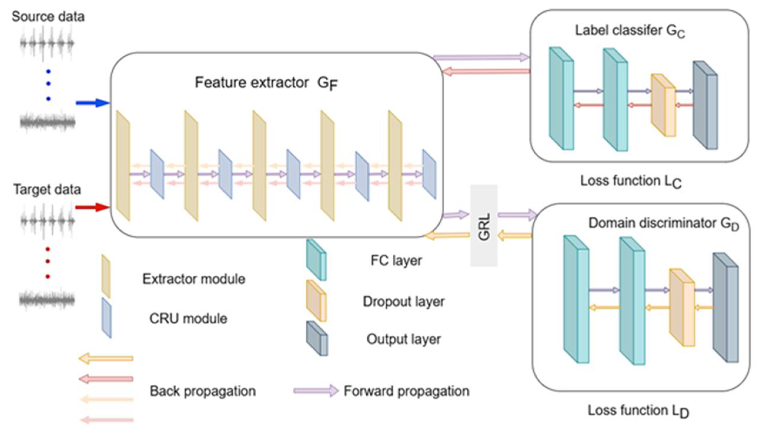
Figure 2.
Structure of feature extractor module
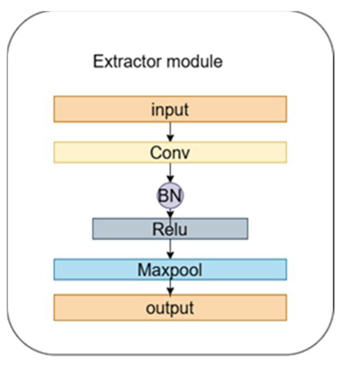
Figure 3.
Structure of CRU
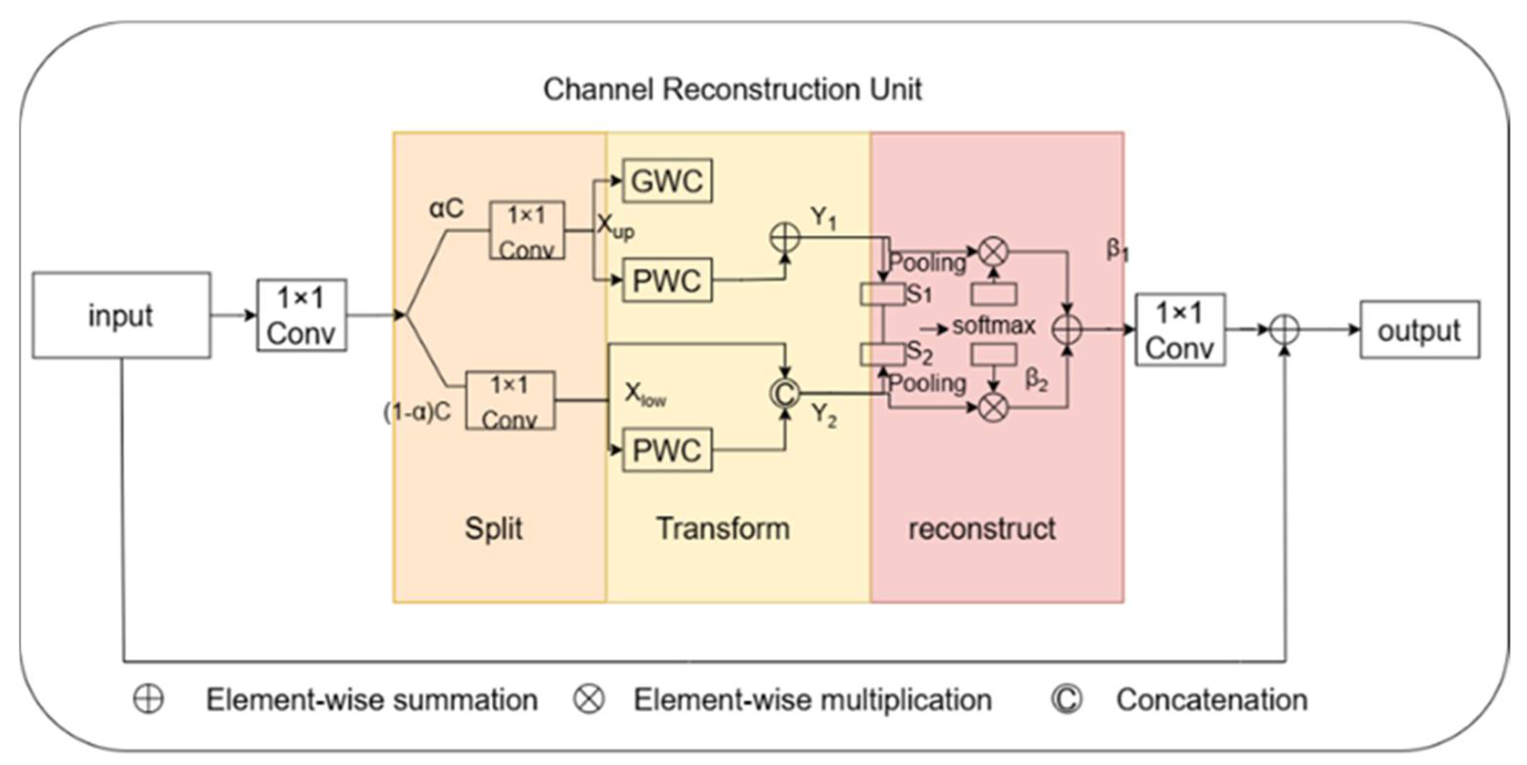
Figure 4.
Time-domain and frequency-domain images of each health state of the bearing
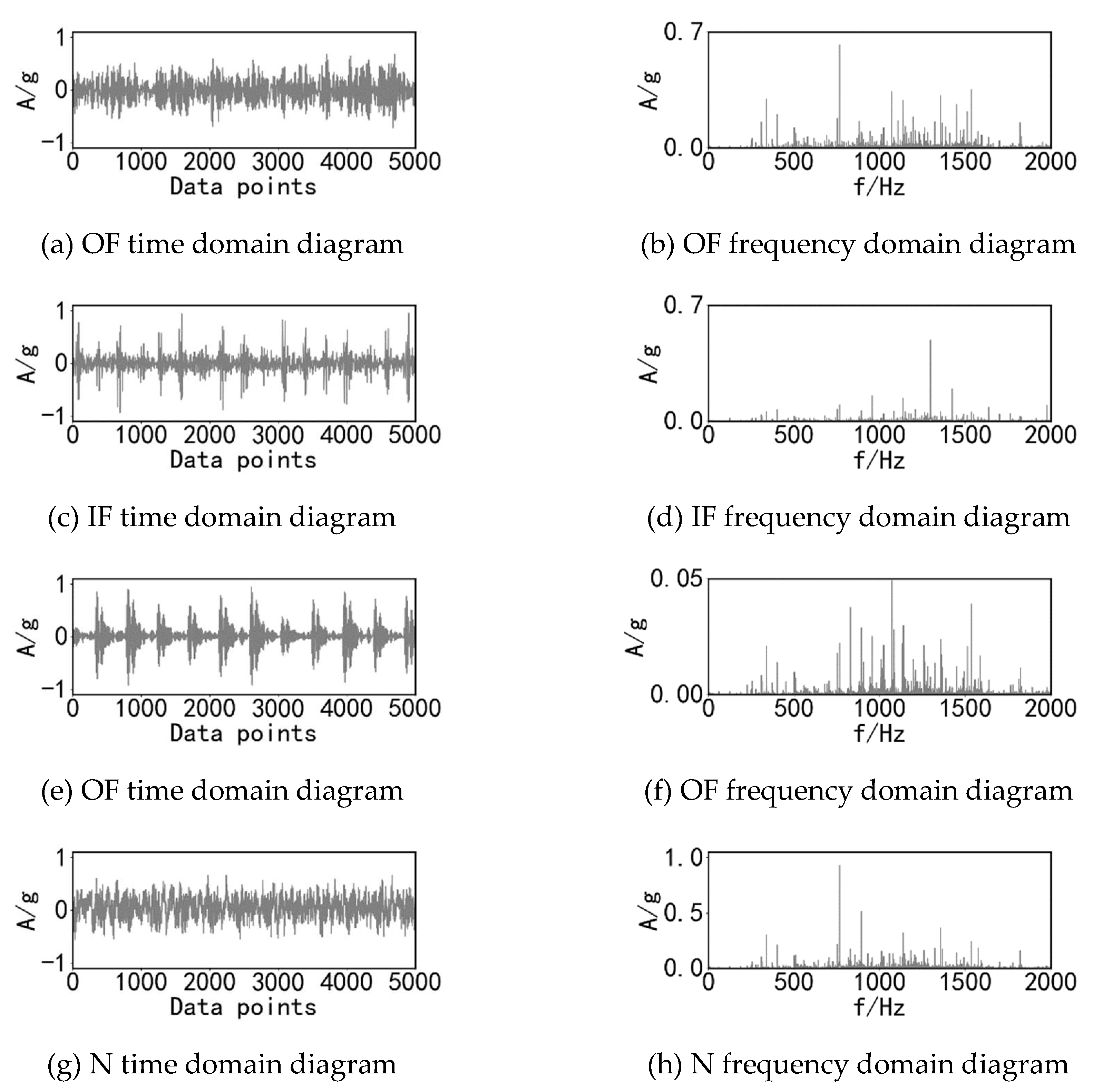
Figure 5.
Visualization of t-SNE for each experimental result
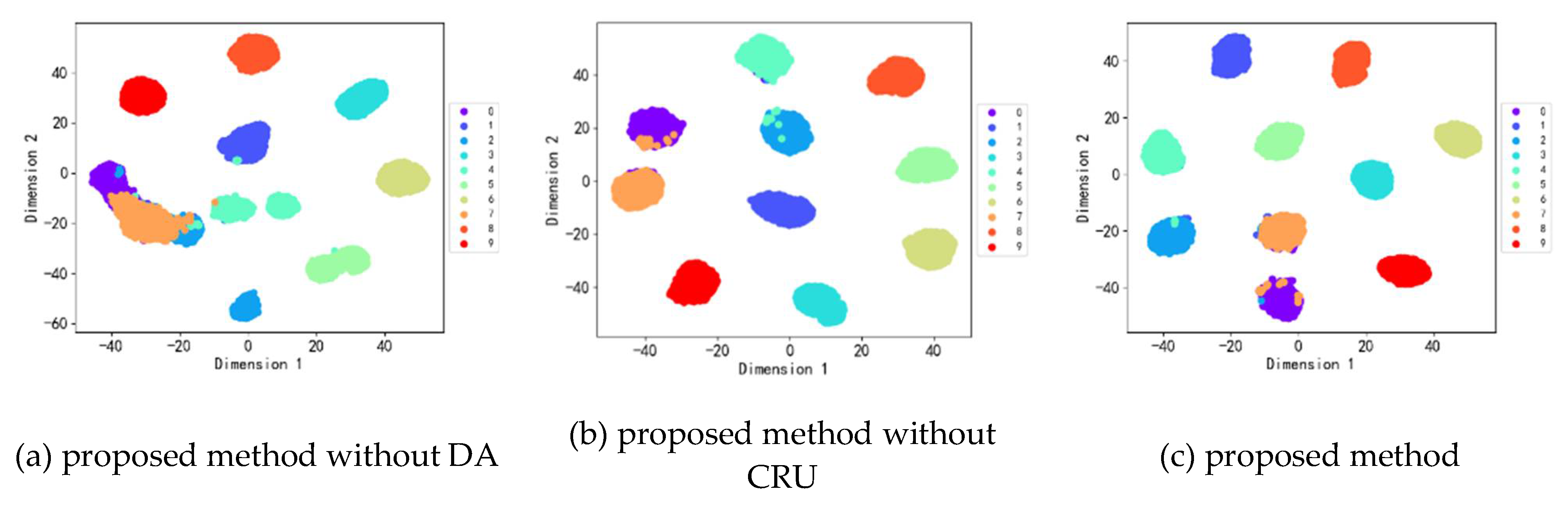
Figure 6.
Confusion matrix for each experimental result
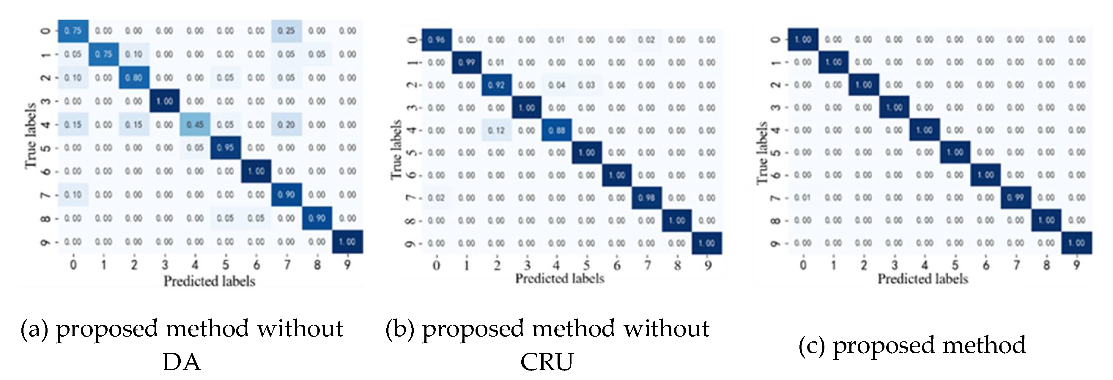
Figure 7.
LY-GZ-02 laboratory bench
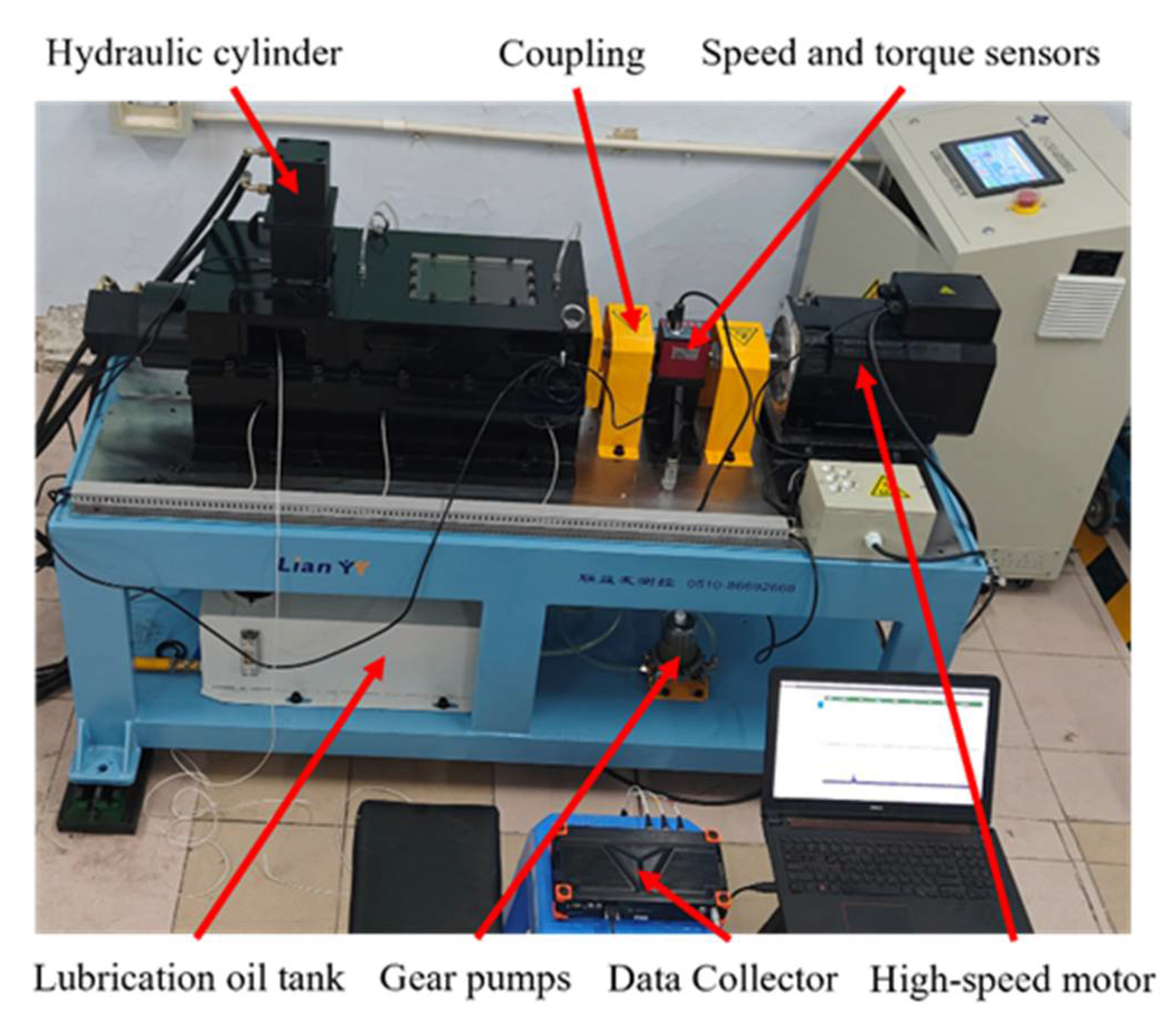
Figure 8.
Time-domain and frequency-domain images of four health states of Skf6007 bearings
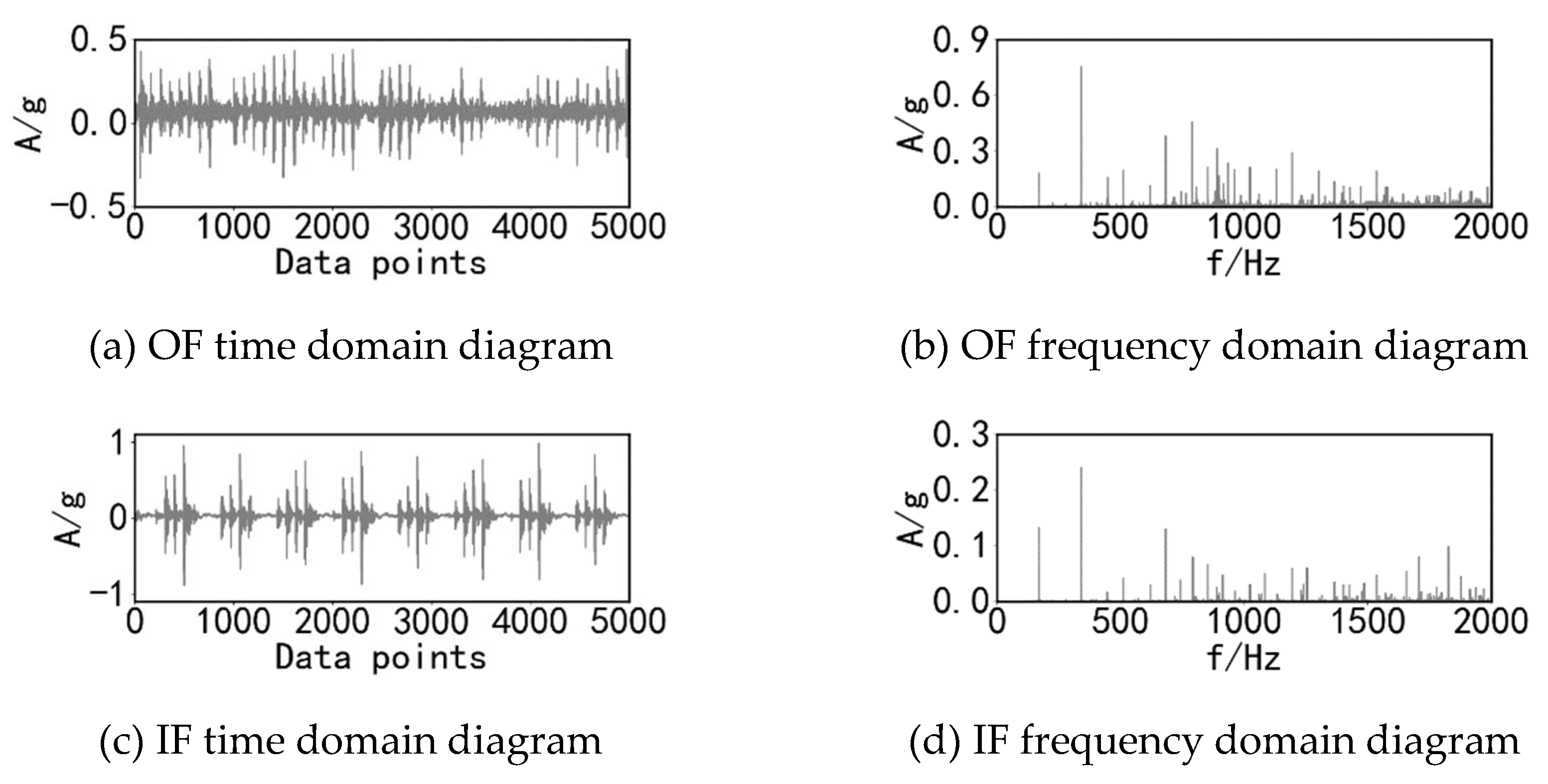
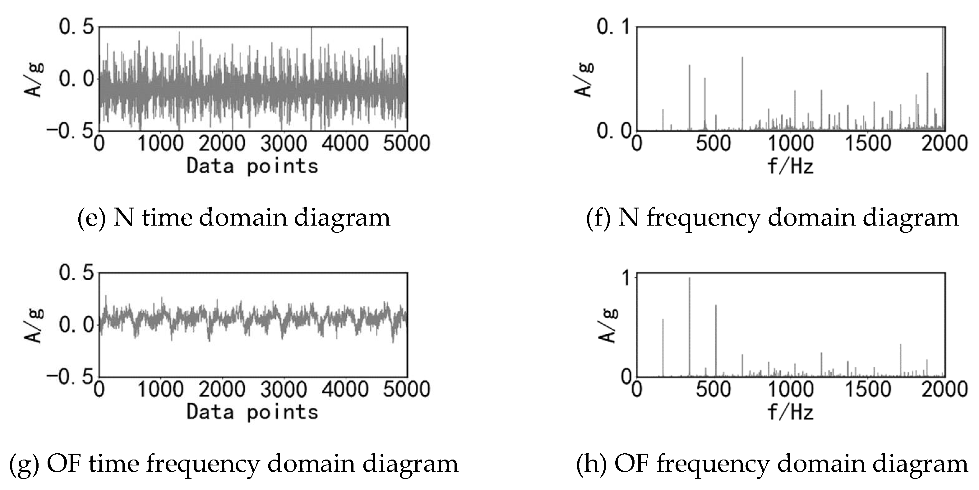
Figure 9.
Confusion matrix for each experimental method
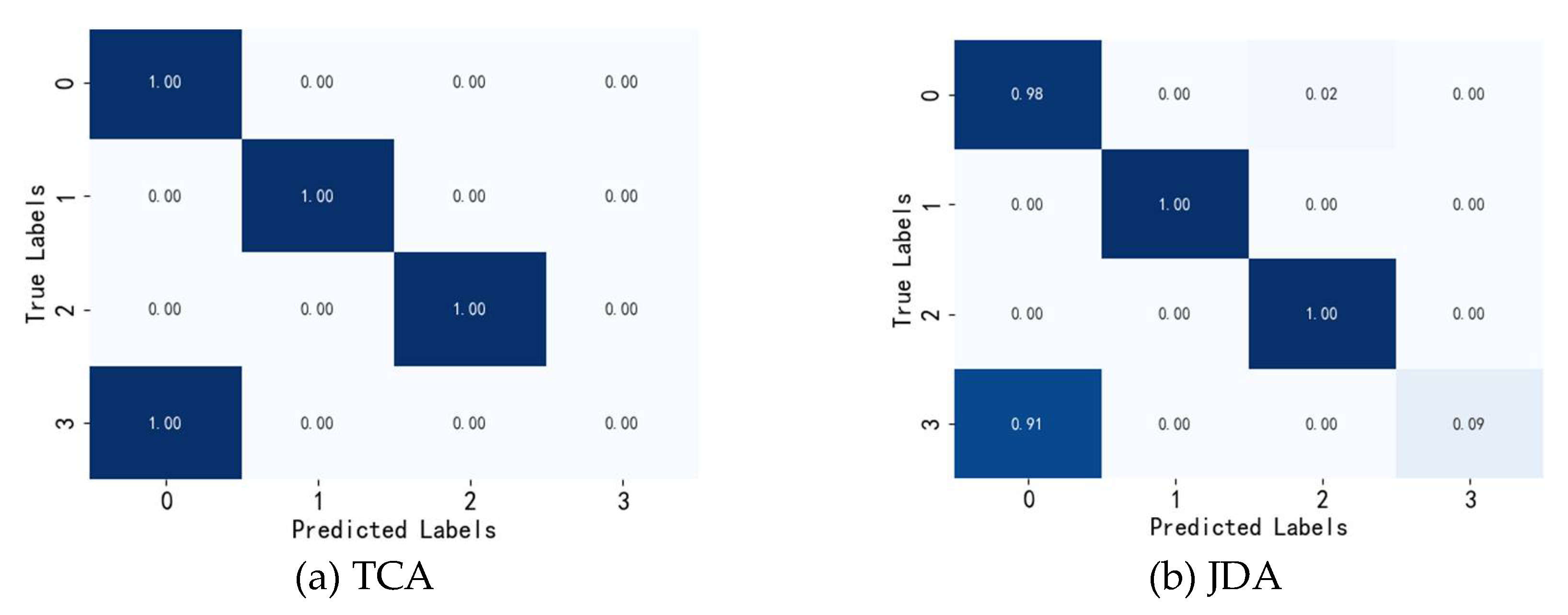
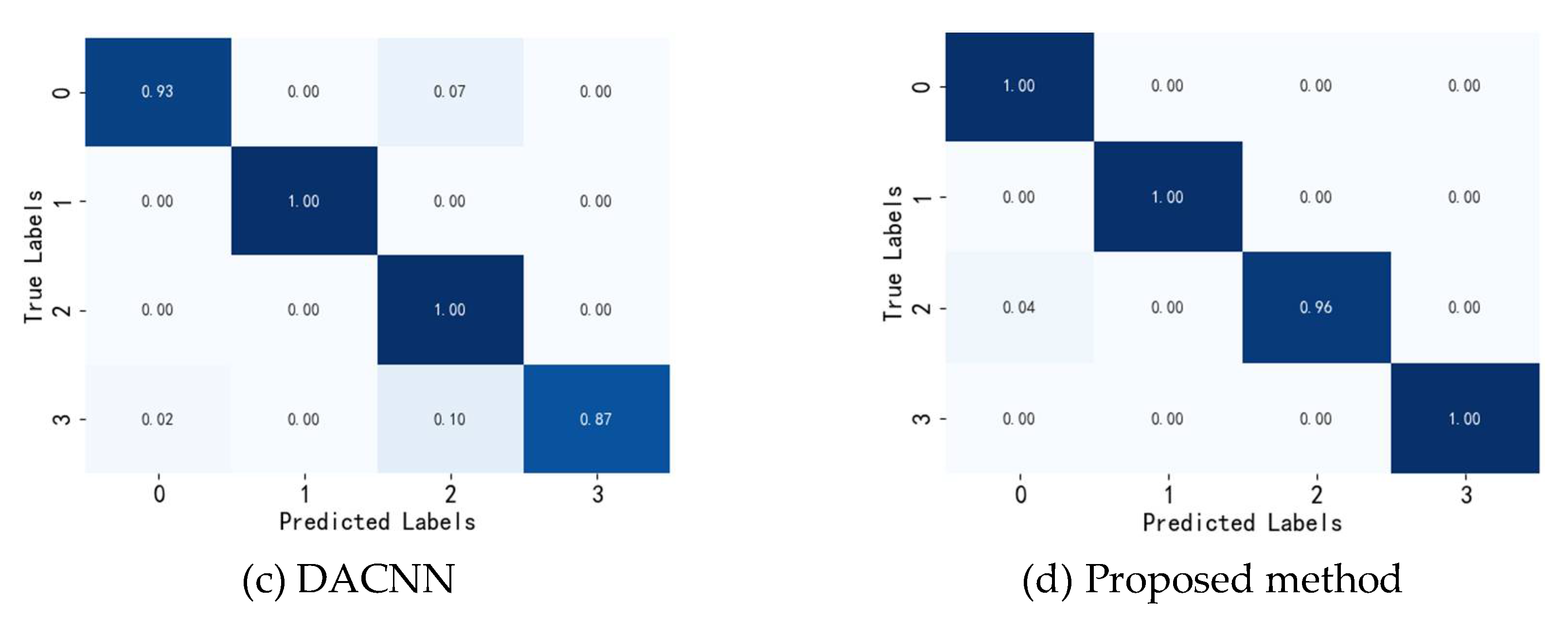

Table 1.
Structural parameters of the characterization module
| Module Sequence | Structural parameters |
| First feature extraction module | Cov1d(64×1,64)+BN(64)+ RELU + Maxpool(2,2) |
| Second feature extraction module | Cov1d(3×1,32) +BN(32)+ RELU + Maxpool(2,2) |
| Third feature extraction module | Cov1d(3×1, 64) +BN(64)+ RELU + Maxpool(2,2) |
| Fourth feature extraction module | Cov1d(3×1, 32) +BN(64)+ RELU + Maxpool(2,2) |
| Fifth feature extraction module | Cov1d(3×1, 64) +BN(64)+ RELU + Maxpool(2,2) |
Table 2.
Datasets description of different operating conditions
| Condition | Rotation speed/(r/min) | Load | Sample size | Sample length |
| A | 1797 | 1hp | 40000 | 1024 |
| B | 1797 | 2hp | 40000 | 1024 |
| C | 1797 | 3hp | 40000 | 1024 |
Table 3.
Dataset settings
| Fault type | Degree of damage | Sample size | 标签 |
| N | None | 2000 | 9 |
| IF | 0.007inch | 2000 | 8 |
| 0.014inch | 2000 | 7 | |
| 0.021inch | 2000 | 6 | |
| OF | 0.007inch | 2000 | 5 |
| 0.014inch | 2000 | 4 | |
| 0.021inch | 2000 | 3 | |
| RF | 0.007inch | 2000 | 2 |
| 0.014inch | 2000 | 1 | |
| 0.021inch | 2000 | 0 |
Table 4.
Test results for each method under each task
| Task | No DA | No CRU | Proposed method |
| A-B | 82.5% | 97.2% | 99.1% |
| A-C | 87.1% | 97.3% | 99.4% |
| B-A | 85.3% | 98.3% | 99.6% |
| B-C | 81.7% | 94.58% | 98.6% |
| C-A | 85.4% | 96.4% | 99.1% |
| C-B | 83.2% | 95.8% | 99% |
Table 5.
Experimental results for different FC layer counts under the A-C migration task
| Structure | Epoch | Accuracy |
| One FC layers + dropout + output | 1000 | 83.5% |
| Two FC layers + dropout + output | 1000 | 99.4% |
| Three FC layers + dropout + output | 1000 | 93.2% |
Table 6.
Testing results of different methods
| Method | A-B | A-C | B-A | B-C | C-A | C-B | Average accuracy |
| SDAE+JGSA28 | 93.4% | 90.1% | 90% | 93.8% | 91.2% | 94.7% | 92.2% |
| DDC29 | 98.4% | 95.7% | 97.7% | 98.3% | 88.5% | 96.7% | 95.9% |
| DACNN30 | 97.3% | 98.3% | 96.2% | 98.1% | 98.1% | 98.4% | 97.7% |
| Proposed method | 99.1% | 99.4% | 99.6% | 98.6% | 99.1% | 99% | 99.3% |
Table 7.
Descriptions of the dataset
| Condition | Fault type | Label | Sample size | Load |
| A | RF | 0 | 1000 | 0N |
| IF | 1 | 1000 | ||
| N | 2 | 1000 | ||
| OF | 3 | 1000 | ||
| B | RF | 0 | 1000 | 1000N |
| IF | 1 | 1000 | ||
| N | 2 | 1000 | ||
| OF | 3 | 1000 | ||
| C | RF | 0 | 1000 | 2000N |
| IF | 1 | 1000 | ||
| N | 2 | 1000 | ||
| OF | 3 | 1000 |
Table 8.
Testing results of different methods
| Method | A-B | A-C | B-A | B-C | C-A | C-B | Average accuracy |
| TCA | 76.9% | 75.1% | 74.2% | 77.5% | 74.4% | 78.3% | 76.1% |
| JDA | 75% | 74.4% | 76.3% | 76.5% | 73.3% | 76.7% | 75.4% |
| DACNN | 95.8% | 96.7% | 94.5% | 97.5% | 94.5% | 97.3% | 96.1% |
Disclaimer/Publisher’s Note: The statements, opinions and data contained in all publications are solely those of the individual author(s) and contributor(s) and not of MDPI and/or the editor(s). MDPI and/or the editor(s) disclaim responsibility for any injury to people or property resulting from any ideas, methods, instructions or products referred to in the content. |
© 2024 by the authors. Licensee MDPI, Basel, Switzerland. This article is an open access article distributed under the terms and conditions of the Creative Commons Attribution (CC BY) license (http://creativecommons.org/licenses/by/4.0/).
Copyright: This open access article is published under a Creative Commons CC BY 4.0 license, which permit the free download, distribution, and reuse, provided that the author and preprint are cited in any reuse.


