Submitted:
21 June 2024
Posted:
24 June 2024
You are already at the latest version
Abstract
Drought stress severely affects the normal growth and development of wheat, leading to reduced yields and quality. To address the lag and limitations of traditional drought monitoring methods, this paper proposes a drought stress monitoring model for winter wheat during critical growth stages based on deep learning. By acquiring drought stress images of winter wheat during three critical growth stages: rise-jointing, heading-flowering and flowering-maturity, a dataset correlating these images with soil moisture monitoring data was established. The DenseNet121 network model was selected as the base network to extract phenotypic features of winter wheat under drought stress. Variables such as the model's training approach, changes in learning rate, and whether an attention mechanism was included, were used to conduct eight sets of model training and optimization strategy experiments. A drought stress monitoring model for winter wheat during critical growth stages based on an improved DenseNet-121 was constructed. The results showed that the average recognition accuracy of the eighth group in the test set reached 94.67%, indicating good application prospects in the recognition of drought stress levels during critical growth stages of wheat.
Keywords:
Optimization strategy
; DenseNet-121
; winter wheat
; drought monitoring
1. Introduction
Wheat is one of the three most important cereals, with approximately 70% of the global wheat cultivation area located in arid and semi-arid agricultural zones[1]. Statistics indicate that China experiences droughts an average of 7.5 times annually, resulting in an average afflicted crop area ranging from 20 to 30 million hm2, leading to an average annual grain reduction of 250-300 billion hm2. This poses significant challenges to grain production and security[2]. The impact of drought on wheat yield and quality depends on factors like the severity and duration of the drought, the timing, and location. Research has shown that the extent of wheat yield reduction is not only related to the degree of drought stress but also to the growth stage during which the drought occurs[3]. Particularly during the wheat jointing, heading, and grain-filling stages, drought stress can severely impact wheat growth and yield levels, reducing its output and quality[4]. Therefore, obtaining real-time wheat drought monitoring data, accurately identifying drought stress in wheat, and swiftly implementing effective irrigation measures to prevent drought exacerbation are fundamental for ensuring wheat drought early warning and mitigation, playing a crucial role in enhancing grain output.
Traditional drought monitoring methods include agricultural meteorological drought monitoring, soil moisture measurement, thermal infrared imaging techniques, hyperspectral imaging, chlorophyll fluorescence techniques, and manual diagnostics. While these methods can evaluate crop drought, they all have inherent delays or limitations to some degree[5]. In agricultural irrigation areas, agricultural meteorological drought monitoring information is somewhat restricted. Irrigation can change soil moisture conditions but cannot promptly alter the humidity and temperature in meteorological monitoring systems[6]. Conversely, soil moisture monitoring is a common indirect method, but due to its limited coverage and accuracy, its application is somewhat constrained[7]. To directly monitor crop drought stress based on affected bodies, researchers employ thermal infrared imaging, hyperspectral imaging, and chlorophyll fluorescence techniques to diagnose and monitor the moisture condition of the canopy and leaves[8]. For instance, Meng Y et al. used thermal infrared imaging analysis of maize drought resistance, analysis of different genotypes of wheat canopy temperature parameters related information, to explore rapid and efficient selection of winter wheat drought-resistant varieties indicators and methods [9]. Mangus et al. leveraging high-resolution thermal infrared images, deeply explored the relationship between canopy temperature and soil moisture[10]. While thermal infrared technology can provide crop drought stress information by monitoring canopy air temperature differences, its spatial coverage is restricted, and it is also influenced by environmental conditions and crop varieties[11]. Hyperspectral technology reflects crop stress states through spectral features[12], extensively used in crop drought stress monitoring, with the drought-sensitive band typically between 1200nm-2500nm[13]. Chlorophyll fluorescence is sensitive to early crop drought stress, but monitoring severe drought stress with chlorophyll fluorescence parameters proves challenging. The current chlorophyll fluorescence technology is primarily restricted to studies on small plants or crops in their seedling stage.
Currently, monitoring large crops or in-field crop phenotypes remains a challenging task. However, with the continuous development of computer vision and image processing technologies, deep learning methods based on two-dimensional digital images have been widely employed for the identification and classification of both biotic and abiotic crop stresses[14]. Deep learning is an image recognition method that combines image feature extraction and classification. Compared to traditional machine learning, it can automatically extract image features, achieving higher recognition accuracy, and more accurately and objectively identifying and grading stresses. Furthermore, deep learning models have been proven to surpass previous image recognition techniques[15], with extensive research indicating their high recognition accuracy and broad application advantages[16,17]. Although some progress has been made in drought stress phenotype research, diagnosing crop drought stress using a single phenotype characteristic remains somewhat limited. Using multi-source sensors to capture crop phenotype information, integrating the color, texture, morphology, and physiological parameters of the crop, and combining pattern recognition algorithms for non-destructive, accurate rapid diagnosis and monitoring of crop drought stress are important future directions.
Therefore, this study selects the DenseNet121 network model as the base to extract phenotypic features under winter wheat drought stress. Using the model's training mode, the change in learning rate, and the presence or absence of attention mechanisms as variables, a total of eight combination experiments are conducted for model training and optimization strategies, constructing a winter wheat key growth stage drought stress recognition model based on DenseNet-121.
2. Datasets and Methods
2.1. Data Preparation
In the experiment, the setting of drought levels at three key growth stages of wheat was referenced from the "Field Survey and Grading Technical Specifications for Winter Wheat Disaster" Part One: Winter Wheat Drought Disaster (NY/T 2283-2012) of the People's Republic of China agricultural industry standard[18]. Three critical growth stages are rise-jointing (RJ), heading-flowering (HF) and flowering-maturity (FM). According to its requirements, drought levels were divided into five levels: Optimum moisture (OM), light drought (LD), moderate drought (MD), severe drought (SD), and extreme drought (ED) as shown in Table 1. Due to the uneven distribution of soil moisture content in the field and the difficulty in accurately controlling irrigation, soil moisture sensors were deployed based on a greedy ant colony algorithm node deployment strategy, with a calibrated accuracy of ±1%. By deploying soil moisture monitoring equipment in the field, data on soil moisture content were obtained. Monitoring devices were used to capture images of wheat under different drought levels (OM, LD, MD, SD, and ED), establishing a drought stress image dataset corresponding to wheat and soil moisture monitoring data.
2.2. Dataset Description
The experiment was conducted from April 2021 to June 2022 at the Agricultural Water Efficiency Laboratory of North China University of Water Resources and Electric Power. Three key growth stages of winter wheat with significant drought stress impact were selected, namely, RJ, HF, and FM. Through real-time monitoring of soil moisture sensors, images of wheat samples under different drought levels at the three key growth stages were collected. After annotation and screening, a total of 12,500 images were used for model training (see Table 2). The image capture time for wheat is shown in Table 3, and samples of winter wheat images are shown in Figure 1.
2.3. Deep Learning Model
The deep learning models selected in this paper are the ones with fewer parameters and higher accuracy trained on the ImageNet dataset, namely, AlexNet, ResNet101, and DenseNet121 as the base network models.
AlexNet, a deep convolutional neural network proposed by Hinton in 2012[19], swept the ImageNet image recognition competition that year. The structure of AlexNet is shown in Figure 2, which includes convolutional layers, pooling layers, fully connected layers, and an output layer. Several convolutional and pooling layers are alternately stacked, followed by two fully connected layers and one output layer. AlexNet led the development of deep learning in the field of computer vision. It pioneered the use of deep convolutional neural networks for image classification and laid the foundation for subsequent deep learning models.
ResNet (Residual Network) is a convolutional neural network model proposed by Kaiming He et al. in 2015[20]. By introducing residual connections, it addresses the vanishing and exploding gradient problems encountered during the training of deep networks. The network structure of ResNet-50 is shown in Figure 3, characterized by its use of residual learning. By introducing "residual blocks", it addresses the gradient vanishing and model degradation issues[21], enabling the network to learn deeper feature representations. ResNet101, with its deeper layers and stronger expressive power, is suitable for complex visual recognition tasks. The advent of ResNet greatly advanced the development of deep learning, making it possible to train deeper neural networks and achieving significant performance improvements in various tasks.
DenseNet (Densely Connected Convolutional Network) is a deep convolutional neural network structure proposed by Gao et al. in 2019[22]. As shown in Figure 4 of the DenseNet series network structure, unlike traditional convolutional neural networks, the output of each layer in DenseNet is connected to the output of all previous layers, forming a densely connected structure. This connection method allows for more efficient feature transfer within the model, effectively reducing the vanishing gradient problem, and improving the model's training efficiency and generalization capability. DenseNet-121 consists of 121 layers. This network adopts a novel structure, making it both concise and efficient, showing better performance on the CIFAR index than the residual network (ResNet).
3. Selection of Basic Deep Learning Mode
3.1. Model Test Environment and Evaluation Metrics
3.1.1. Test Environment
The configuration of the computer used for the test is shown in Table 4.
3.1.2. Model Evaluation Metrics
During the model training process, the values of hyperparameters such as optimizers and learning rates usually need to be adjusted continuously. When selecting a convolutional neural network model, the best-performing model from multiple hyperparameter sets is chosen as the final model. This ensures optimal performance and efficiency for the model.
This research uses multiple indicators to evaluate the winter wheat drought stress identification and classification model, including the Accuracy of drought stress identification (A1), Precision of drought stress classification (P1), and the comprehensive evaluation indicator F1 value. A1 assesses the accuracy of drought identification, P1 evaluates the classification results, and F1 is the harmonic mean of precision and recall, evaluating the model's recognition accuracy for wheat drought images, combining the advantages of both.
1)Accuracy (A1) refers to the proportion of samples correctly classified by the classifier to the total number of samples. Its formula is:
2) Precision (P1) refers to the proportion of actual positive samples in the samples predicted to be positive for each category. Its formula is:
3) Recall (R1) represents the proportion of positive samples in each category predicted as positive. The formula is:
4) The F1 value is a comprehensive evaluation indicator. It is the harmonic mean of precision and recall. A higher F1 value indicates better classifier performance. The F1 value formula is:
Where: TP represents the number of positive samples predicted as positive by the model. TN represents the number of negative samples predicted as negative by the model. FP represents the number of actual positive samples predicted as negative. FN represents the number of actual negative samples predicted as positive.

Table 5.
The confusion matrix for determining whether the classification of winter wheat is correct based on the recognition model.
Table 5.
The confusion matrix for determining whether the classification of winter wheat is correct based on the recognition model.
| Label Category | Model Prediction | ||
|---|---|---|---|
| 0 | 1 | ||
| Truth Label | 0 | True positive(TP) | False negative(FN) |
| 1 | False positive(FP) | True negative(TN) | |
3.2. Training Method of Deep Learning Model
Convolutional neural networks require extensive training to seek optimal hyperparameters. With different hyperparameters as variables, multiple control experiments are conducted. The design is as follows: First, three convolutional neural networks: ResNet-101, DenseNet-121, and AlexNet were employed to build a wheat drought stress classification identification model, and the model is trained from scratch. During the training process, all data is divided into training and test sets, randomly distributed at an 8:2 ratio, where 80% of the samples are used for model training, and 20% for model testing. During model training, the learning rate decay method is set to fixed (Fixed), with a learning rate of 0.001, optimizer set to Stochastic Gradient Descent (SGD), and a batch size of 100. Firstly, the model's convergence is judged by comparing the model's loss function, and at the same time, by comprehensively comparing indicators such as recognition accuracy and F1 value, the basic network model with the best generalization ability on this dataset is selected. Secondly, after selecting the basic network model, a total of 8 combination experiments are carried out with training methods, learning rate, and attention mechanism as variables, comprehensively comparing the model's recognition accuracy and F1 value indicators, to find the most suitable convolutional neural network model and corresponding hyperparameters
3.3. Training Method of Deep Learning Model
In this section, ResNet-101, DenseNet-121, and AlexNet convolutional neural networks are used to build the wheat drought stress classification identification model respectively. The model's generalization capability is judged by accuracy and F1 value, and the model's convergence is verified by the loss function, thereby selecting the network model with the best generalization capability on this dataset as the basic model. The experimental results of the evaluation indicators of the three deep learning models are shown in Table 6. Figure 5 displays the loss values, accuracy, and F1 values of ResNet-101, DenseNet-121, and AlexNet convolutional neural networks on the test set.
From Table 6, it can be observed: In terms of drought identification accuracy, the DenseNet-121 model has the highest precision with an accuracy of 87.60% on the test set. ResNet-101 and AlexNet models have accuracies of 74.80% and 55.83% respectively. Judging from the model's loss function and F1 value, the convergence speed of the DenseNet-121 model is faster than that of the ResNet-101 and AlexNet models, and the ResNet-101 model exhibits overfitting. The F1 value of the DenseNet-121 model is 0.8729, higher than the 0.7173 and 0.5326 of the ResNet-101 and AlexNet models respectively. In a comprehensive comparison, the DenseNet-121 network model is chosen as the experimental basic network model.
4. Model Optimization Strategies and Result Analysis
4.1. Model Optimization Strategy
This section is based on the DenseNet121 network model. Using the training method of the convolutional neural network model, the changing condition of the learning rate, and the addition of the attention mechanism as variables, 8 combination experiments were conducted in total. The results of the training are summarized in Table 7.
4.2. Result Analysis
4.2.1. Impact of Transfer Learning on the Model
To explore the impact of transfer learning on model training, several comparison experiments were designed under the same learning rate and attention mechanism. Specifically, Experiments 1, 2, 3, 4 were compared with Experiments 5, 6, 7, 8. The comparative results of Experiment 1 & 5 and Experiment 4 & 8 are shown in Figure 6. As shown, the accuracy rates of Experiment 1 and 5 are 75.87% and 90.27%, respectively, and the F1 scores are 0.7581 and 0.8535. The accuracy rates of Experiment 4 and 8 are 87.00% and 94.67%, respectively, with F1 scores of 0.8536 and 0.9438. The accuracy and F1 scores of models using transfer learning techniques both improved. This indicates that: ① Fine-tuning all layers performs better; ② Compared to fine-tuning only the last layer, models that fine-tune all layers achieve a significant increase in accuracy. This suggests that the dataset used in this study differs significantly from the ImageNet dataset in terms of feature characteristics. Fine-tuning all layers can integrate feature learning, share knowledge, and provide a larger network capacity, adapting better to the target task's requirements.
4.2.2. Impact of Gradient Learning Rate on the Model
To investigate the impact of the change in learning rate on the model training outcomes, under the conditions where the transfer learning method and attention mechanism remain consistent, several control experiments were designed, namely Experiments 1, 2, 5, 6 and Experiments 3, 4, 7, 8. The comparison results of Experiment 1 and 3, and Experiment 6 and 8 are shown in Figure 7. From the figure, it can be seen that the accuracy of Experiment 1 and Experiment 3 are 75.87% and 82.33% respectively, with F1 scores of 0.7581 and 0.8110 respectively. The accuracy of Experiment 6 and Experiment 8 are 91.20% and 94.67% respectively, with F1 scores of 0.9087 and 0.9438 respectively. The accuracy and F1 values of the model have been improved after using the gradient learning rate. It can be concluded that: ① The model using the gradient learning rate has slightly higher recognition accuracy than the one with a constant learning rate. In Experiment 1 and Experiment 3, the average recognition accuracy increased significantly. This indicates that the gradient learning rate method can effectively manage and adjust the learning speed of the model during the training process, allowing the model to use a larger learning rate in the initial stage for faster convergence, and gradually reduce the learning rate in the subsequent stages. This enables the model to fine-tune its parameters more delicately, thereby enhancing its generalization performance. In contrast, the model with a fixed learning rate may experience overfitting or underfitting in the early or later stages, resulting in subpar overall performance. ② The gradient learning rate method can better balance the model's learning speed at different training stages. In deep learning models, the learning rates of different layers may have different impacts on model performance. The gradient learning rate method can adjust the learning rates of different layers according to the specific task and network structure, allowing the model to learn and update the parameters of each layer more effectively, thereby enhancing the model's expressiveness. In contrast, the model with a fixed learning rate may not fully utilize the hierarchical features of the network structure, thus affecting the recognition accuracy. In this section, the initial learning rate is set to 0.001, and the learning rate is halved every 10 epochs.
4.2.3. Impact of the Attention Mechanism on the Model
To investigate the impact of the attention mechanism on the model training results, under the conditions where the transfer learning method and the learning rate remain consistent, several control experiments were designed, namely Experiments 1, 3, 5, 7 and Experiments 2, 4, 6, 8. The comparison results of Experiment 1 and 2, and Experiment 5 and 6 are shown in Figure 8. From the figure, it can be seen that the accuracy of Experiment 1 and Experiment 2 are 75.87% and 79.87% respectively, with F1 scores of 0.7581 and 0.7894 respectively. The accuracy of Experiment 5 and Experiment 6 are 90.27% and 91.20% respectively, with F1 scores of 0.9015 and 0.9087 respectively. The introduction of the attention mechanism has improved the model's accuracy and F1 values. It can be concluded that: ①Introducing the attention mechanism module can weight the importance of winter wheat to enhance the model's focus on its features and improve the model's ability to perceive the importance of different features. In deep learning models, the quality and importance of feature representations have a significant impact on the performance of the task. By introducing the attention mechanism, the model can dynamically adjust the weights and contributions of the features, allowing the model to focus more on key information and enhance the expression of the features. In contrast, models that do not incorporate an attention mechanism may fail to accurately distinguish the importance of different features, leading to suboptimal performance. ②Introducing the attention mechanism can enhance the model's perception of the importance of different time steps or spatial positions. In deep learning models, for sequential problems or tasks with spatiotemporal structures, the information from different time steps or spatial positions has varying importance. By using the attention mechanism, the model can dynamically adjust the importance weights of different time steps or spatial positions, better capturing the features of sequences or spatiotemporal patterns. Compared to models that do not use attention mechanisms, models that incorporate attention can better leverage temporal or spatial information, enhancing the performance of deep learning models.
4.3. Experimental Results Validation
The confusion matrix[23] is one of the factors used to evaluate the model. It is a heatmap in matrix form, where rows represent the actual category labels and columns represent the predictions. The confusion matrices for the results of experiment 1, experiment 4, and experiment 8 are derived through calculations, as shown in Figure 9. Analyzing Figure 9, we can discern: ① In the three different growth stages of wheat, certain stages are mistakenly identified as other stages. For instance, the "RJ" stage is sometimes wrongly identified as the "HF" stage. This is because the growth of wheat is a continuous process. As it transitions from the "RJ" stage to the "HF" stage, features like stem, leaves, and texture do not undergo significant changes in comparison to the "HF" stage. ② Adjacent drought levels within the same growth cycle are also easily confused. For instance, the appropriate state might be mistakenly determined as mild drought, mild drought may be wrongly classified as either appropriate or moderate drought, moderate drought might be mistakenly identified as mild or severe drought, and severe drought may be mistakenly identified as extreme drought. This is because drought stress is a continuous, dynamic accumulation process where the phenotypic differences of wheat plants under adjacent drought levels are minimal with unclear boundaries. ③ With continuous model improvements, misjudgments are alleviated. Especially evident from the confusion matrix of experiment 8, misjudgments are limited to the "RJ" stage. This is due to the minimal physiological and morphological phenotypic differences of wheat under drought stress during this stage, leading to potential misidentification. Therefore, by utilizing transfer learning, gradual learning rate adjustments, and the introduction of the attention mechanism, this section aims to enhance the drought identification accuracy of winter wheat, thereby refining the ability to determine drought stress during the wheat growth process.
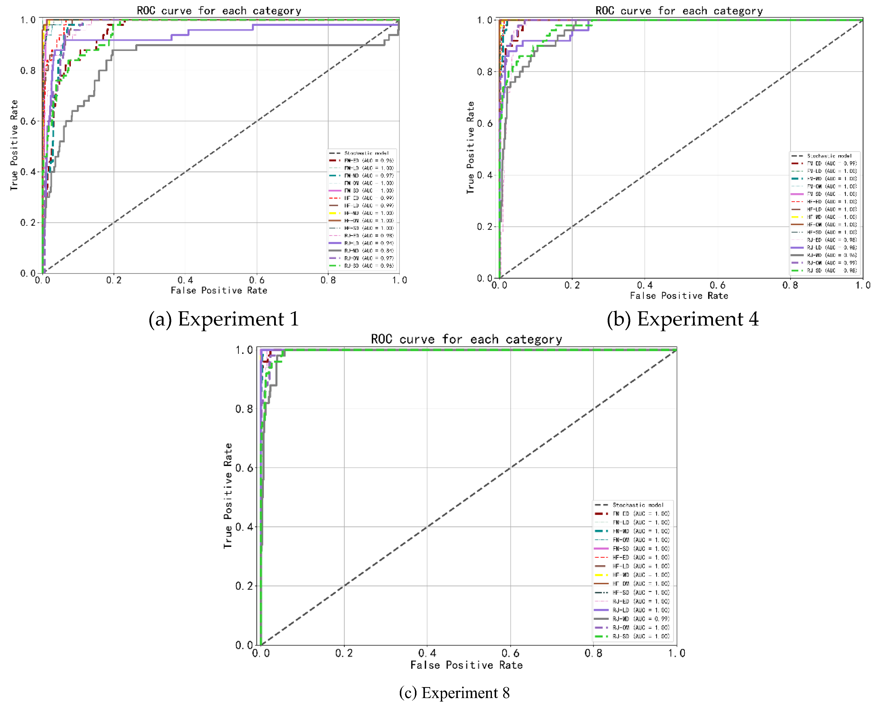
The Receiver Operating Characteristic (ROC) [23] is one of the factors used to evaluate the model. The X-axis of the horizontal coordinate of the ROC curve is the False Positive Rate (FPR), also known as the False Diagnosis Rate (FDR). As shown in equation (5), so the closer the X-axis is to zero, the higher the accuracy; the vertical coordinate Y-axis is the True Positive Rate, TPR, also known as the sensitivity, as shown in equation (6), the larger the Y-axis represents the higher the accuracy. AUC (Area under Curve, AUC) denotes the area under the ROC curve, which is mainly used to measure the model generalization performance, i.e., how well the classification is done. i.e. how good the classification is. It indicates the probability that positive examples are ranked in front of negative examples. Generally in classification models, the prediction results are expressed in the form of probability.
In addition, with the help of AUC, we discover that the false positive rate was considerably lower in the improved model compared to the unimproved model. Off in terms of both accuracy and AUC, the improved model performs better than the unimproved, and for trials 1 and 8, the AUC under RJ-MD classification increased by 15%. When the improved methods were compared with each other, the migration learning method that took the approach of fine-tuning the training of all layers, the asymptotic learning rate method, and the model that introduced the attention mechanism performed the best in terms of AUC and specificity. In conclusion, the improved model outperforms the pre-improved model in all aspects.
Figure 10.
ROC curves for different experimental results.
In this section, we explored the impacts of transfer learning methods and learning rates on model performance and investigated the effects of the attention mechanism on model training results. Experimental results show that fine-tuning all layers rather than just the final layer can further enhance model performance; models using a gradual learning rate method slightly outperform those with a fixed learning rate, indicating that the gradual learning rate method effectively manages and adjusts the learning rate of the model. Introducing an attention mechanism to models slightly improves recognition accuracy over models without it. This is because the attention mechanism enhances the model's weighted importance of wheat features and focuses on key information, improving the model's perception of importance across different features, time steps, and spatial positions. In this section, by leveraging the feature extraction capabilities of pre-trained models, dynamically adjusting learning rates, and enhancing attention to vital information and its importance, we aim to elevate the detection performance, accuracy, and generalization ability of the model. These strategies, applied across diverse tasks and network structures, can significantly boost the generalization capabilities of deep learning models. The integrated application of these methods in this section can improve the training results and generalization ability of the model, speed up model convergence, and enhance performance metrics such as recognition accuracy. Specifically, the test set's average recognition accuracy for experiment 8 reached 94.67%, demonstrating promising potential in recognizing drought levels during critical wheat growth stages.
5. Conclusions
This paper introduces a drought monitoring model for the growth process of winter wheat based on deep learning, aiming to identify and classify the degree of drought stress during the critical growth stages of winter wheat. We focused on three key growth periods of winter wheat: RJ, HF and FM to study drought stress. We collected images of winter wheat drought stress from field conditions during these periods and established a drought image set corresponding to soil moisture monitoring data. By comparing the drought stress recognition accuracy, classification accuracy, recall rate, and F1 value of the AlexNet, ResNet-101, and DenseNet-121 network models, the DenseNet-121 network model was chosen as the base model for this chapter. Building upon the selected DenseNet-121, we developed training and optimization strategies for the model, considering improvements like the use of transfer learning, the adoption of a gradual learning rate, and the introduction of the attention mechanism method. Eight experimental groups were carried out. The results indicate that through these improvements, the model's convergence speed is accelerated, and performance metrics, including recognition accuracy, are enhanced. This effectively improves the identification and classification of drought stress levels during the key growth stages of winter wheat. Notably, the test set's average recognition accuracy for experiment 8 reached 94.67%.
A comprehensive analysis reveals that deep learning algorithms provide a more reliable and accurate method for identifying and classifying the degree of wheat drought. This method has extensive application prospects in agricultural production, resource allocation, and other areas, offering reliable scientific support for decision-making.
Author Contributions
This research was a collaborative effort with each author contributing significantly to various aspects of the study. Jianbin Yao was instrumental in developing the Methodology, ensuring the study's approach was both robust and relevant. Yushu Wu took the lead in preparing the Writing—Original Draft, meticulously crafting the initial manuscript that laid the foundation for our work.Jianhua Liu provided essential Supervision throughout the project, guiding the research team with his expertise and ensuring the study met the highest academic standards. Hansheng Wang contributed by creating insightful Visualizations, effectively communicating complex data and findings in a clear and accessible manner.Each author has played a pivotal role in the research process, and all have read and agreed to the final published version of the manuscript. The authorship is attributed only to those who have made substantial contributions to the work as reported..
Funding
The work was supported by Major Science and Technology Projects of the Ministry of Water Resources(Grant No.SKS-2022029), Projects of Open Cooperation of Henan Academy of Sciences(Grant No.220901008), the Key Scientific Research Projects of Henan Higher Education Institutions(No.24A520022) and the North China University of Water Conservancy and Electric Power High-level experts Scientific Research foundation(202401014).
Data Availability Statement
We are committed to the principles of open science and data sharing. The data supporting the findings of our study are available in the public domain for the benefit of the scientific community. Specifically, the dataset used in our research, which pertains to the drought monitoring study of key growth stages of winter wheat based on multimodal deep learning, can be accessed through the following link: Minimal dataset for multimodal deep learning. This dataset includes wheat drought stress images, soil, and meteorological data, which were integral to our analysis. We encourage readers and fellow researchers to explore and utilize this dataset for further studies and applications.
Acknowledgments
The work was supported by Major Science and Technology Projects of the Ministry of Water Resources(Grant No.SKS-2022029), Projects of Open Cooperation of Henan Academy of Sciences(Grant No.220901008), the Key Scientific Research Projects of Henan Higher Education Institutions(No.24A520022) and the North China University of Water Conservancy and Electric Power High-level experts Scientific Research foundation(202401014).
Conflicts of Interest
The authors declare no conflicts of interest. We affirm that there were no personal circumstances or interests that could have inappropriately influenced the representation or interpretation of the reported research results.Furthermore, we wish to clarify that the funders had no role in the design of the study; in the collection, analyses, or interpretation of data; in the writing of the manuscript; or in the decision to publish the results. The independence of the research process and the integrity of the findings have been maintained throughout, ensuring that the conclusions drawn are solely based on the evidence presented.
References
- Mustafa, H.; Ilyas, N.; Akhtar, N.; et al. Biosynthesis and characterization of titanium dioxide nanoparticles and its effects along with calcium phosphate on physicochemical attributes of wheat under drought stress. Ecotoxicology and Environmental Safety 2021, 223, 112519. [Google Scholar] [CrossRef] [PubMed]
- Cao, Y.Q.; Lu, J.; Feng, X.X. Risk zoning of drought damage for spring maize in northwestern Liaoning. Journal of Natural Resources 2021, 36, 1346–1358. [Google Scholar] [CrossRef]
- Wang, J.; Xiong, Y.; Li, F.; et al. Effects of Drought Stress on Morphophysiological Traits, Biochemical Characteristics, Yield, and Yield Components in Different Ploidy Wheat: A Meta Analysis. Advances in Agronomy 2017, 139–173. [Google Scholar]
- Torres, G.M.; Lollato, R.P.; Ochsner, T.E. Comparison of Drought Probability Assessments Based on Atmospheric Water Deficit and Soil Water Deficit. Agronomy Journal 2013, 105, 428. [Google Scholar] [CrossRef]
- Zhou, J.; Francois, T.; Tony, P.; et al. Plant phenomics: Development, current situation and challenges. Journal of Nanjing Agricultural University 2018, 580–588. [Google Scholar]
- Zhang, Y.; Wang, Z.; Fan, Z.; et al. Phenotyping and evaluation of CIMMYT WPHYSGP nursery lines and local wheat varieties under two irrigation regimes. Breed Sci 2019, 69, 55–67. [Google Scholar] [CrossRef]
- Feng, C.H.; Wu, J.L.; Liu, X.L.; et al. Modeling and Prediction of Soil Moisture Content at Field-Scale Based on ln-situ Soil Spectroscopy. Chinese Journal of Soil Science 2020, 51, 1374–1379. [Google Scholar]
- Yang, N.; Deng, S.L.; et al. Research Progress in Agricultural Drought Monitoring Based on Multi-source Information. Journal of Catastrophology 2023, 1–17. [Google Scholar]
- Meng, Y.; Wen, P.F.; Ding, Z.Q.; et al. Identification and Evaluation of Drought Resistance of Wheat Varieties Based on Thermal Infrared Image. Scientia Agricultura Sinica 2022, 55, 2538–2551. [Google Scholar]
- Mangus, D.L.; Sharda, A.; Zhang, N. Development and evaluation of thermal infrared imaging system for high spatial and temporal resolution crop water stress monitoring of corn within a greenhouse. Computers and Electronics in Agriculture 2016, 121, 149–159. [Google Scholar] [CrossRef]
- Khanal, S.; Fulton, J.; Shearer, S. An overview of current and potential applications of thermal remote sensing in precision agriculture. Computers and Electronics in Agriculture 2017, 139, 22–32. [Google Scholar] [CrossRef]
- Baret, F.; Madec, S.; Irfan, K.; et al. Leaf-rolling in maize crops: From leaf scoring to canopy-level measurements for phenotyping. Journal of Experimental Botany 2018, 69, 2705–2716. [Google Scholar] [CrossRef] [PubMed]
- Wang, H.; Qian, X.; Zhang, L.; et al. A Method of High Throughput Monitoring Crop Physiology Using Chlorophyll Fluorescence and Multispectral Imaging. Frontiers in Plant Science 2018, 9, 407. [Google Scholar] [CrossRef]
- Singh, A.K.; Ganapathysubramanian, B.; Sarkar, S.; et al. Deep Learning for Plant Stress Phenotyping: Trends and Future Perspectives. Trends in Plant Science 2018, 23, 883–898. [Google Scholar] [CrossRef] [PubMed]
- Kamilaris, A.; Prenafeta-Boldú, F.X. Deep learning in agriculture: A survey. Computers and Electronics in Agriculture 2018, 147, 70–90. [Google Scholar] [CrossRef]
- Ma, J.; Du, K.; Zheng, F.; et al. A recognition method for cucumber diseases using leaf symptom images based on deep convolutional neural network. Computers and Electronics in Agriculture 2018, 154, 18–24. [Google Scholar] [CrossRef]
- Veeramani, B.; Raymond, J.W.; Chanda, P. Deep Sort: Deep convolutional networks for sorting haploid maize seeds. BMC Bioinformatics, 2018, 19, 289–296. [Google Scholar] [CrossRef]
- NY/T2283-2012. Technical specification for field survey and grading of winter wheat disasters [S]. Beijing: China Agricultural Press, 2012.
- Mohammed, S.; Matta, N.; et al. Coronavirus Pneumonia Classification Using X-Ray and CT Scan Images With Deep Convolutional Neural Network Models. Journal of Information Technology Research 2022, 15, 1–23. [Google Scholar]
- Zheng, Y.; Wang Yang, J.; et al. Principal characteristic networks for few-shot learning. Journal of Visual Communication and Image Representation 2019, 59, 563–573. [Google Scholar] [CrossRef]
- Wang, H.F.; Shen, Y.Y.; et al. Ensemble of 3D Densely Connected Convolutional Network for Diagnosis of Mild Cognitive Impairment and Alzheimer’s disease. Neurocomputing 2018, 333, 145–156. [Google Scholar] [CrossRef]
- Gao, J.L.; Wang, J.S.; Wang, X. Research on image recognition method based on DenseNet. Journal of Guizhou University (Natural Science Edition) 2019, 36, 58–62. [Google Scholar]
- Dhakshayani, J.; Surendiran, B. M2F-Net: A Deep Learning-Based Multimodal Classification with High-Throughput Phenotyping for Identification of Overabundance of Fertilizers. Agriculture 2023, 1238, 1–19. [Google Scholar] [CrossRef]
Figure 1.
Sample of some winter wheat.
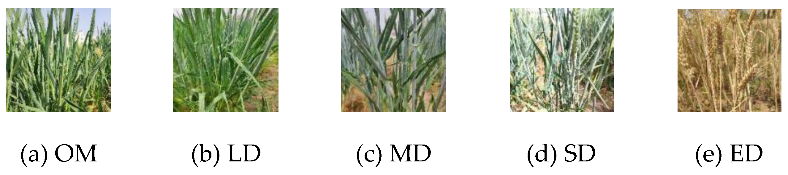
Figure 2.
AlexNet network structure diagram.
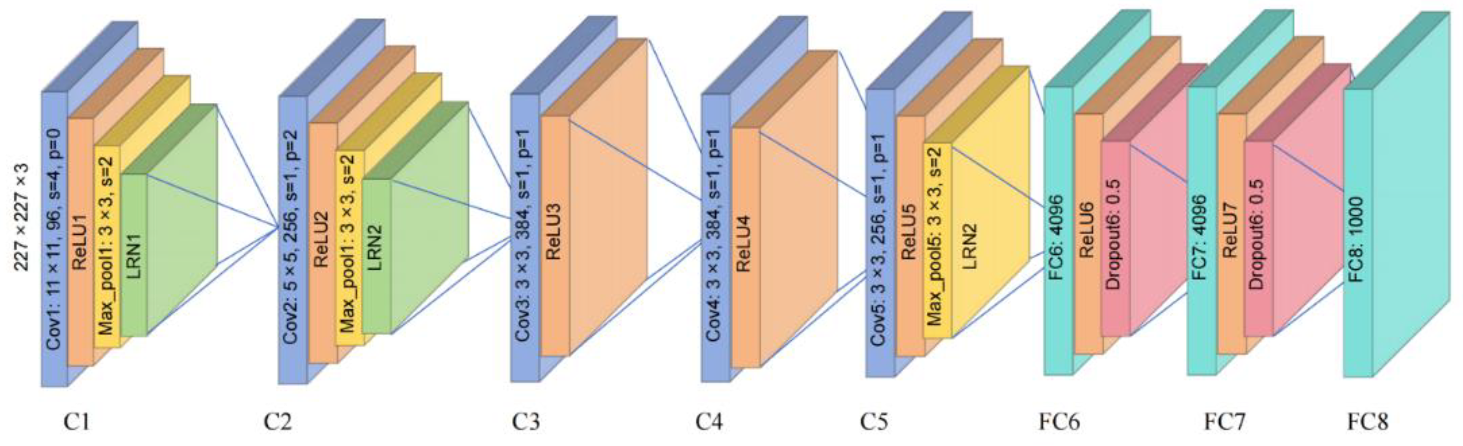
Figure 3.
ResNet-50 network structure diagram.
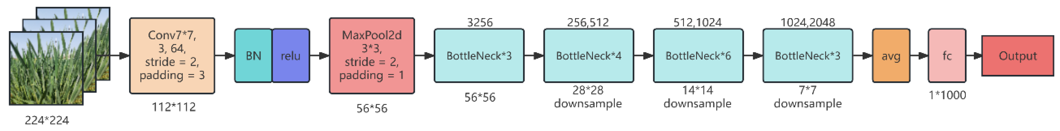
Figure 4.
DenseNet network structure diagram.
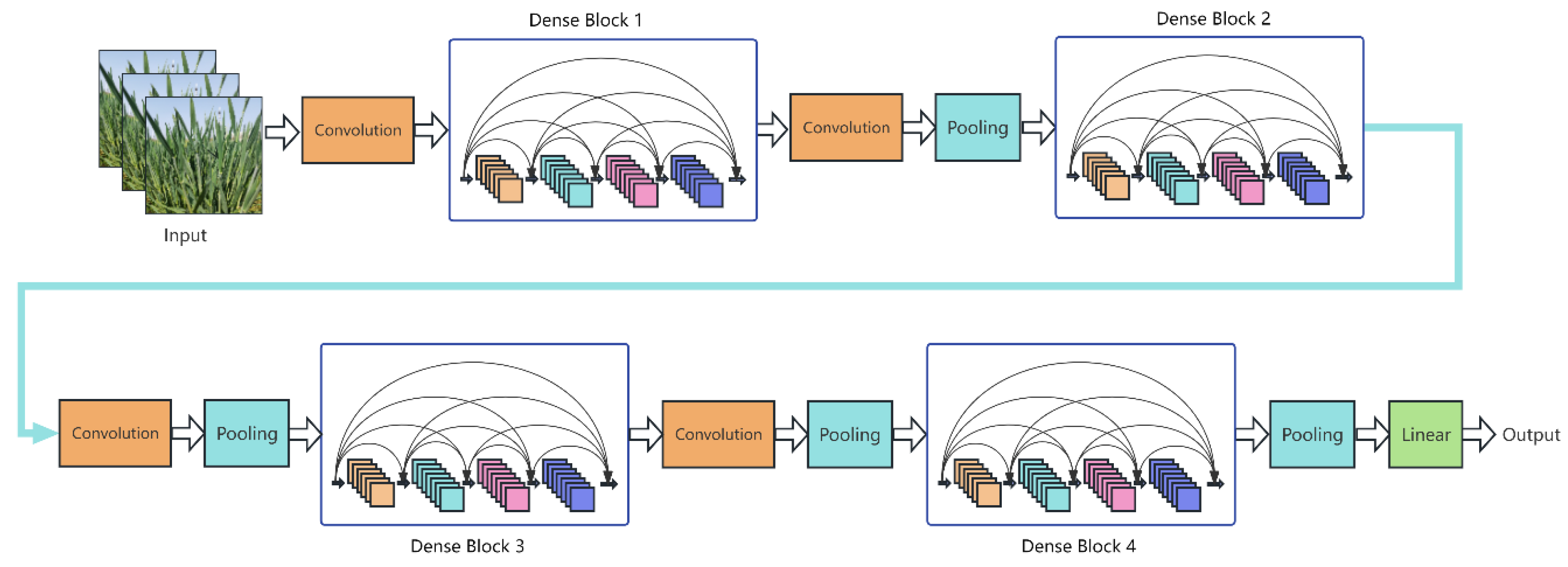
Figure 5.
Loss values, accuracy, and F1 values of differentdeep learning models on the test set.
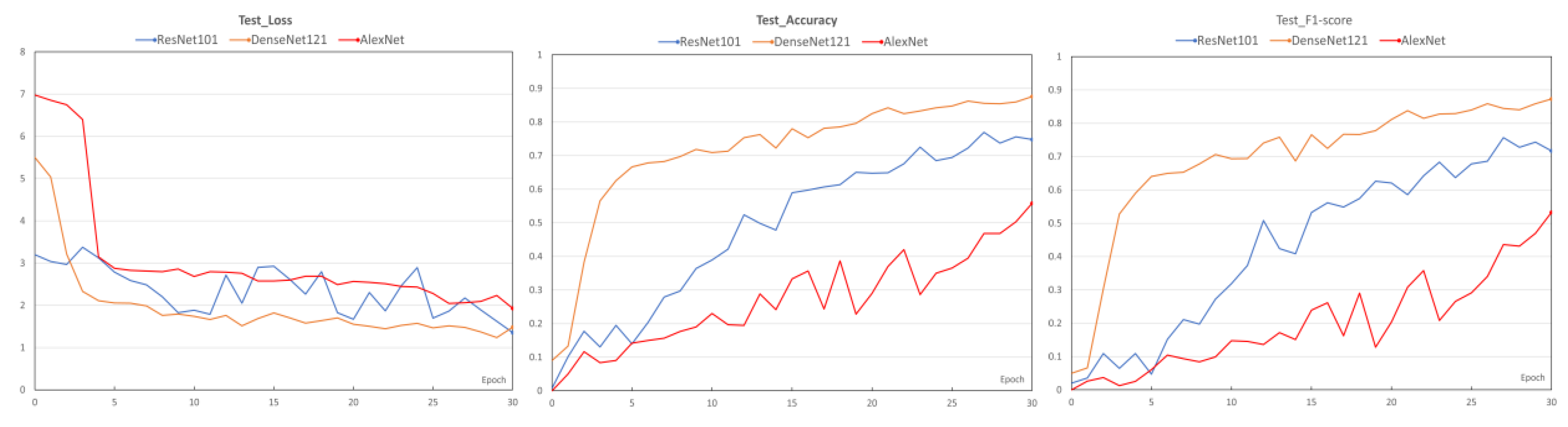
Figure 6.
Control chart of experimental results with and without transfer learning.
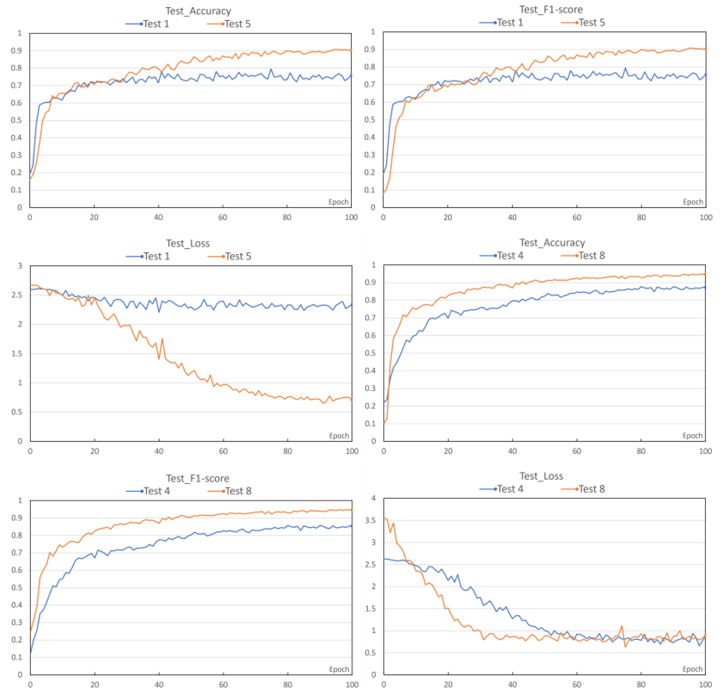
Figure 7.
Control chart of experimental results with and without asymptotic learning rate.
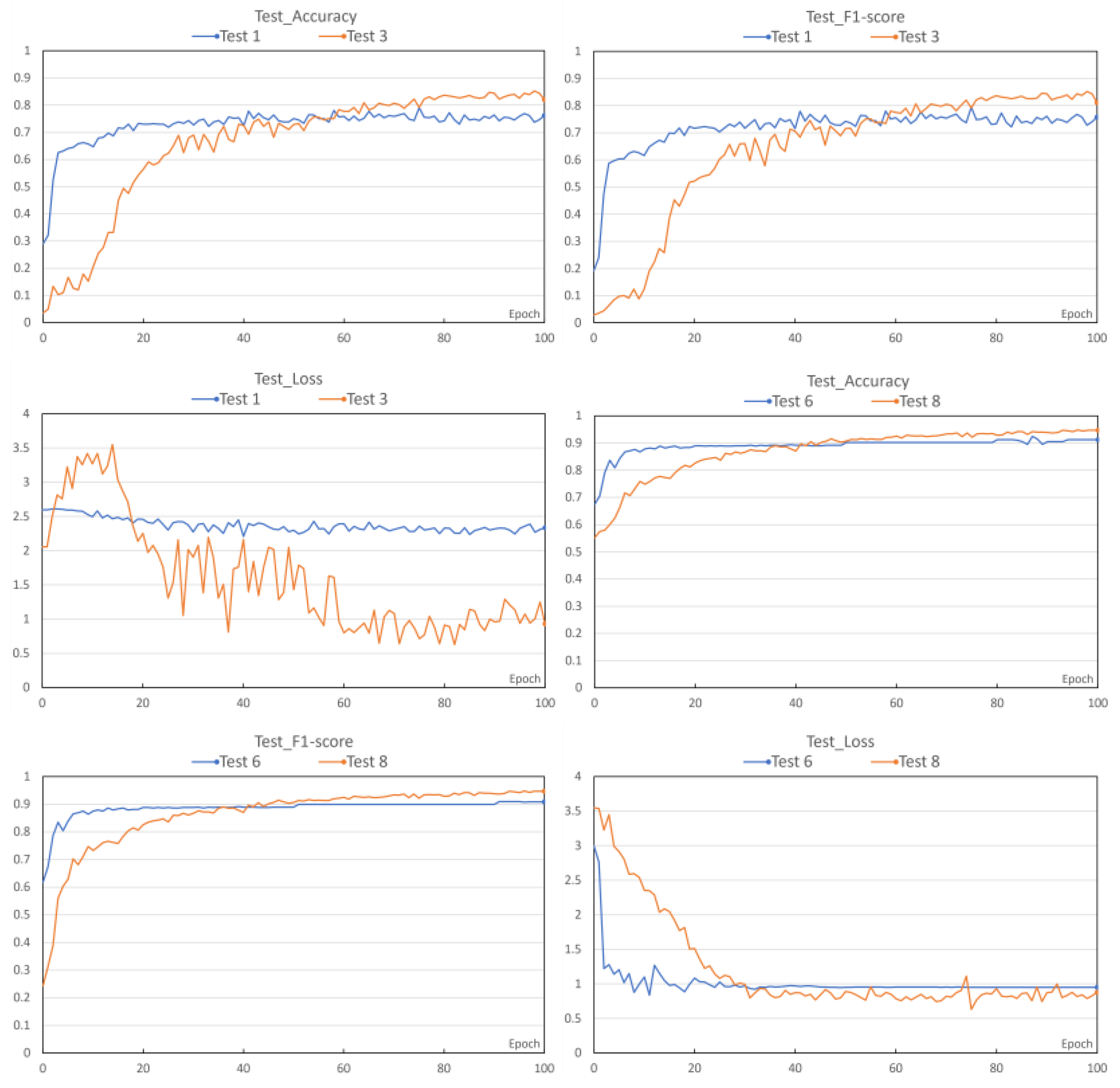
Figure 8.
Control chart of experimental results with and without the introduction of an attention mechanism.
Figure 8.
Control chart of experimental results with and without the introduction of an attention mechanism.
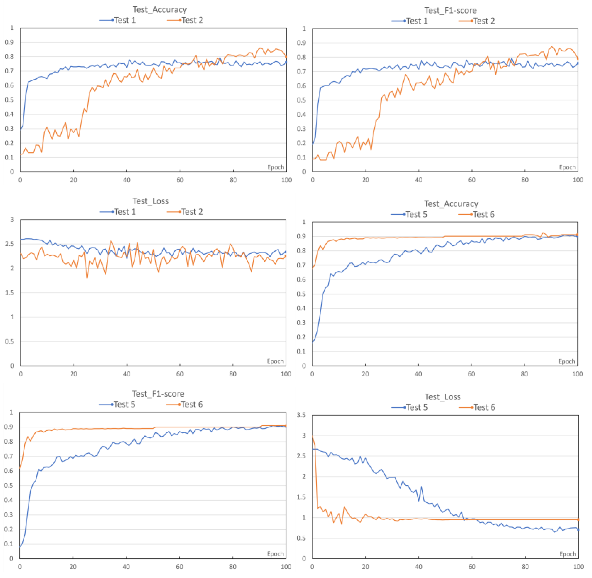
Figure 9.
Confusion matrix for different experimental results.
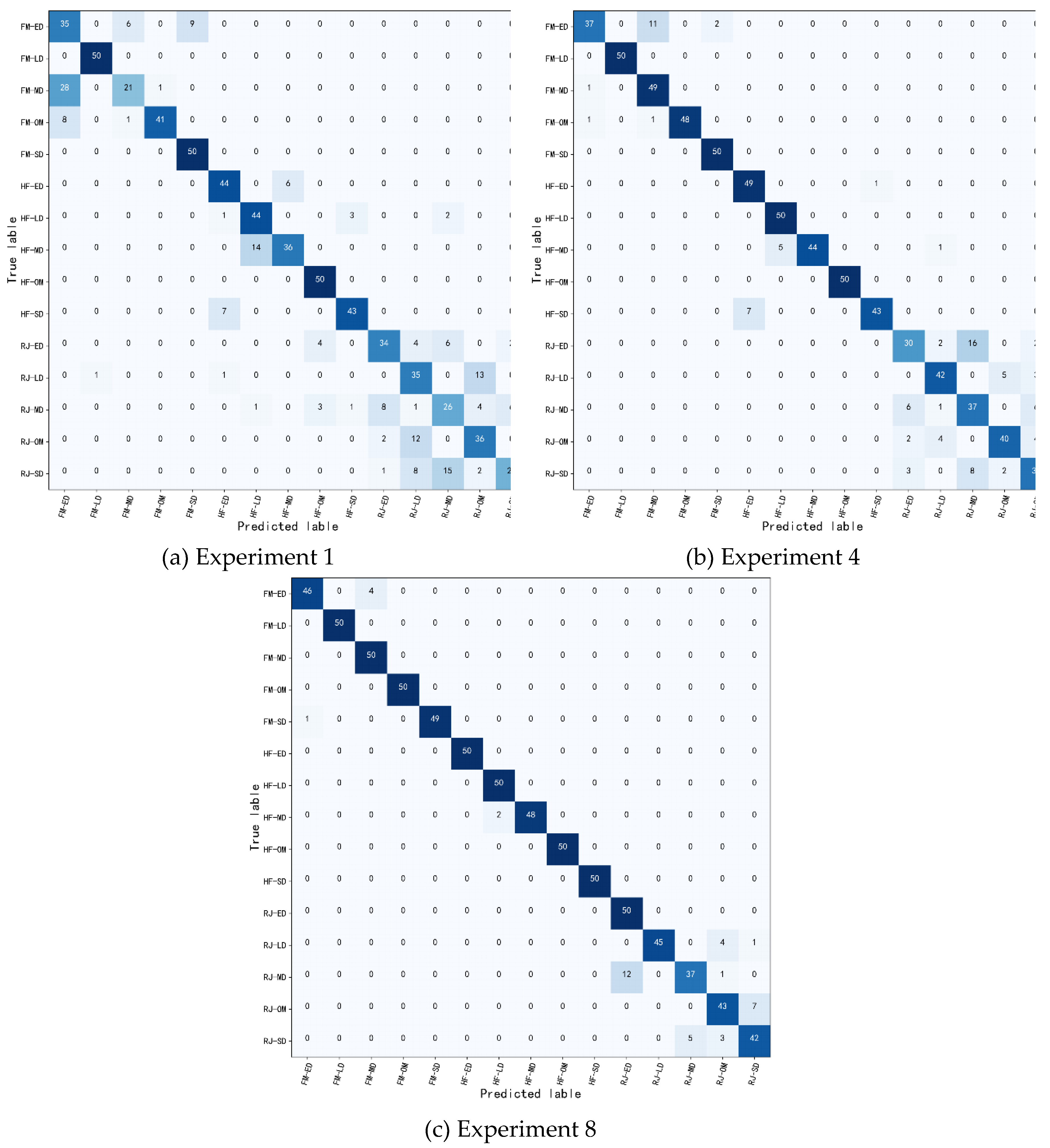
Table 1.
Standards for drought levels of wheat at different growth stages.
| Drought Level | RJ | HF | FM |
|---|---|---|---|
| OM | >65%FC | >70%FC | >70%FC |
| LD | 60%≤~<65%FC | 65%≤~<70%FC | 65%≤~<70%FC |
| MD | 55%≤~<60%FC | 60%≤~<65%FC | 60%≤~<65%FC |
| SD | 45≦~<55%FC | 55≤~<60%FC | 55≤~<60%FC |
| ED | <40%FC | <45%FC | <45%FC |
Note: FC (field capacity) is the field water holding capacity.
Table 2.
Image quantity table of wheat growth stages under different drought levels.
| Growth Stage | OM | LD | MD | SD | ED | Total Data |
|---|---|---|---|---|---|---|
| RJ | 950 | 900 | 880 | 820 | 650 | 4200 |
| HF | 900 | 840 | 840 | 845 | 775 | 4200 |
| FM | 1220 | 920 | 850 | 720 | 490 | 4100 |
Table 3.
Acquisition time of wheat drought images.
| Year | RJ(Month/Day) | HF (Month/Day) | FM (Month/Day) |
|---|---|---|---|
| 2021 | 04.03-04.23 | 04.24-05.02 | 05.03-05.23 |
| 2022 | 03.29-04.16 | 04.17-04.30 | 05.01-05.19 |
Table 4.
Acquisition time of wheat drought images.
| Configuration | Information |
|---|---|
| Operating System | Windows11 |
| RAM | 16 GB |
| CPU frequency | 3.20 GHz |
| GPU | NVIDIA GeForce RTX 3060 |
| GPU memory | 6GB |
Table 6.
Basic experimental results of three network models based on test sets.
| Evaluation Metrics | ResNet101 | DenseNet121 | AlexNet |
|---|---|---|---|
| Drought Identification Accuracy | 74.80% | 87.60% | 55.83% |
| Drought Classification Precision | 79.10% | 88.36% | 63.38% |
| Drought Identification Recall | 74.79% | 87.59% | 55.83% |
| F1 value | 0.7173 | 0.8729 | 0.5326 |
Table 7.
DenseNet-121 Network Model Training Results.
| Parameters | Transfer Learning | Gradient Learning Rate | Attention Mechanism | Accuracy | Loss Value | F1 Score |
|---|---|---|---|---|---|---|
| Experiment 1 | × | × | × | 75.87% | 2.3360 | 0.7581 |
| Experiment 2 | × | × | √ | 79.87% | 2.2569 | 0.7894 |
| Experiment 3 | × | √ | × | 82.33% | 0.9301 | 0.8110 |
| Experiment 4 | × | √ | √ | 87.00% | 0.8766 | 0.8536 |
| Experiment 5 | √ | × | × | 90.27% | 0.7059 | 0.9015 |
| Experiment 6 | √ | × | √ | 91.20% | 0.9521 | 0.9087 |
| Experiment 7 | √ | √ | × | 93.87% | 0.9274 | 0.9383 |
Disclaimer/Publisher’s Note: The statements, opinions and data contained in all publications are solely those of the individual author(s) and contributor(s) and not of MDPI and/or the editor(s). MDPI and/or the editor(s) disclaim responsibility for any injury to people or property resulting from any ideas, methods, instructions or products referred to in the content. |
© 2024 by the authors. Licensee MDPI, Basel, Switzerland. This article is an open access article distributed under the terms and conditions of the Creative Commons Attribution (CC BY) license (http://creativecommons.org/licenses/by/4.0/).
Copyright: This open access article is published under a Creative Commons CC BY 4.0 license, which permit the free download, distribution, and reuse, provided that the author and preprint are cited in any reuse.


