Submitted:
20 June 2024
Posted:
21 June 2024
You are already at the latest version
Abstract
Good Boussinesq equations will be considered in this work. First we apply three combined compact schemes to approximate spatial derivatives of good Boussinesq equations. Then three fully discrete schemes are developed based on symplectic scheme in time direction, which are sympletic-structure preserving.Meanwhile, the convergence and conservation of the fully discrete schemes are analyzed. Finally, we present numerical experiments to confirm our theoretical analysis. Both our analysis and numerical test indicate that the fully discrete schemes are efficient in solving the spatial derivative mixed equation.
Keywords:
Hamiltonian system
; good Boussinesq equation
; symplectic scheme
; combined compact scheme
; conservation
1. Introduction
Boussinesq equations are important mathematical physical models in characterizing ocean mixing, atmospheric convection, and intra-Earth convection, which play a key role in fields such as earth sciences, meteorology, and oceanography fields. The study of Boussinesq equation is of great value because it helps us to better understand the hydrodynamic behavior, especially in terms of thermal convection, ocean currents, and atmospheric phenomena. In addition, the study of the Boussinesq equation is essential for the development of numerical models for weather forecasting, climate research, and oceanography. These studies have also helped uncover the fundamental principles that govern fluid motion and heat transfer, contributing to advances in fields such as engineering, environmental science, and geophysics. The GB equation and its various extensions have been extensively analyzed in the existing literature, such as a closed form solution for the two soliton interaction in [1],a highly complicated mechanism for the solitary waves interaction in [2],and the nonlinear stability and convergence of some simple finite difference schemes in [3]. In recent works concerning the numerical solution of PDE, a significant amount addresses the Schrödinger equation, see [4,5,6,7,8,9]. In [9],using a combined compact difference method to solve Schrödinger equation and this scheme is Structure-Preserving.This method originated from [10],it also can be found in[11,12,13,14]. In addition,many works related to GB equations could be found in [15,16,17,18,19,20,21].Higher order Boussinesq equations have been investigated by Z.L. Zou [22].
In solving PDEs numerically, high-order compact (HOC) schemes are often used to discretize spatial derivatives.For example,HOC schemes have been applied to solve steady convection-diffusion equation [12], nonlinear Schrödinger equation [9], Klein-Gordon-Schrö-dinger equation [23], and good Boussinesq equation [17].Compared with general finite difference schemes, HOC schemes have the advantages of smaller error and higher accuracy under the same calculation amount. However, for PDEs with multiple order spatial derivatives, such as good Boussinesq equation , the advantages of classical HOC schemes are often offset. If multiple HOC schemes are used to discretize multiple spatial derivatives simultaneously, it is necessary to perform multiple matrix inverse operations, which will reduce the computational efficiency and affect the accuracy. In [9], Then combined high-order compact (CHOC) scheme is used to approximate PDEs with multiple order spatial derivatives and achieve some discrete conservation laws.
In this paper, three CHOC schemes of good Boussinesq equation are derived. Applying Taylor analysis to an equality combining the solution u and its first derivative, second derivative, and third derivative yields the first three-point CHOC scheme. This scheme has 6th-order precision and has extensive application. Then similarly, we propose the second three-point 8th-order scheme by using a combination of the first,second,third derivatives of the solution. Since the two schemes have a large amount of matrix operations and complex formulation, the third scheme is designed finally by composing the solution and its second derivative, fourth derivative, which greatly simplifies the matrix operations and ensures certain accuracy. In this scheme, through simpler computations, the relationship between the solution and its fourth-order derivative, as well as the relationship between the solution and its second-order derivative can be directly obtained, which can’t be done by first two schemes in this paper. Finally we will use the three schemes to simulate a motion invariant, and summarize the advantages and disadvantages of these schemes. At the same time, compared with a three-point compact scheme with sixth order accuracy derived by Chu and Fan in 1998 [10], our schemes are more accurate.
In this paper, we consider fully discrete schemes for linear good Boussinesq equation
where is a constant. The following nonlinear good Boussinesq equation is also numerically solved
We consider initial conditions and periodic boundary conditions as follows
2. Establishment of the CHOC Scheme
In this paper, we introduce three schemes for discretization of spatial derivatives. To detail the CHOC scheme, we introduce a uniform grid with and First, we introduce the simplest scheme (2.1) and (2.2)
where are coefficients to be determined according to the accuracy of the approximation. The three-point CHOC scheme for the combination of first and second derivatives is to relate to their neighbors . This scheme approximates first-order derivative and second-order derivative of u separately using above combinations by Wang and Kong et al [9].
By inserting Taylor expansion to equation (2.1)and(2.2), we can get the following Table 1 and Table 2.
To make this scheme with sixth order convergence, above coefficients must satisfy the following algebraic equations:
and
The solutions of above equations are
and
Therefore, schemes(2.1) and (2.2) are in the spacific forms
After conducting a thorough analysis, it is determined that this scheme has a relatively limited applicability. Its usage often necessitates complex matrix operations, and it is insufficient for differential equations involving certain high-order derivatives. For Good Boussinesq equation under study in this paper, a fourth-order spatial derivative is involved. To get the numerical solutions of Good Boussinesq equations, we need the discretization of and. Here, we adopt the combination of function values of u and its first-order derivative, second-order derivative to represent fourth-order spatial derivative
Under periodic boundary conditions, by combining (2.5) and (2.6) we have
where
Therefore, we can represent it in the following form:
By solving (2.8), we can obtain: For (2.7) we have
where
By substituting into it, above expression can be represented as follows
Let We will have the following schemes to the spatial derivatives
Next, we will give second CHOC scheme with eighth order accuracy with the combination of first, second and third derivatives relating to their neighbors and . Generalization of (2.1) and (2.2) to the case of three derivatives jields similarly the next CHOC scheme
where are coefficients to be determined according to the accuracy of the approximation. By Taylor expansion of equation(2.11),(2.12) and (2.13) we can get Table 3, Table 4 and Table 5.
To make these schemes of eighth order, they must satisfy the algebraic equations:
and
and
Their unique solutions are
and
and
respectively. Therefore, the scheme (2.11),(2.12) and (2.13) has in the following specific form:
This three-point scheme possesses eighth-order accuracy and involve three derivatives, so it is more applicable and allows for greater accuracy in comparison to (2.1) and (2.2).
Next, we adopt the combination of function values of u and its first three derivatives to represent fourth-order spatial derivative
By Combining (2.17), (2.18), (2.19) and (2.20) we obtain
where
Therefore, we can represent it as follows
In light of solving (2.22), we can obtain: ,
substituting into (2.21) gives that
let we will get the following discrete schemes of the spatial derivative:
For above scheme, we find that matrix operation becomes complicated. To get the discrete form of and according to the (2.11), (2.12) and (2.13), it requires many matrix operations, and subsequent simulation of numerical solution will be more difficult. So we consider constructing a direct combination of and u to look for third CHOC scheme. This scheme will maintain a 6th-order precision and can easily obtain the discrete forms of and , which will be more pertinent and accurate This scheme has the following formulation
We insert Taylor expansions to (2.25) to obtain
To make the scheme with sixth order accuracy, the coefficients must satisfy the algebraic equations
Similarly,for(2.26)we have:
To make the scheme with sixth order accuracy, coefficients must satisfy the algebraic equations
Under periodic boundary conditions, for (2.25) and (2.26), we obtain
where let
Therefore, we can represent it in the following form:
With (2.27), we can readily derive and by expressions of U, respectively. This significantly streamlines the matrix operations. By solving (2.27), we can obtain ,where For good Boussiensq equations, above scheme has higher spatial accuracy compared to the scheme given in [11].
3. Establishment of the Full Discrete Schemes
Let be temporal stepsize and , where . Denote the approximation of by . Define the following operators
Let , the considered good Boussinesq equation can be written as
Applying CHOC scheme (2.10) to the spatial derivatives of above equation gives that
where By adopting symplectic midpoint scheme with second-order accuracy to above equation, we have the following full discrete scheme
Similarly, using CHOC scheme (2.24) for the spatial derivatives yields that
where we obtain the corresponding full discrete scheme
Applying CHOC scheme (2.27) for the spatial derivatives gives that
where we get the following full discrete scheme similarly
By combining (3.2), (3.3), (3.4) with (3.1), respectively, we always obtain the algebraic equation as follows
where A and B are some invertible tridiagonal matrices depending on the corresponding schemes, and F is the corresponding nonlinear term.
For simplicity, we will denote the schemes corresponding to (3.2), (3.3) and (3.4) by CHOC-A, CHOC-B and CHOC-C, respectively.
4. Conservation Laws of CHOC Schemes
Under periodic boundary condition (1.3) with , some good Boussinesq equations have certain conservation laws. Below, we consider periodic domain .
Theorem 4.1.
Let denote the standard -norm for 1-periodic functions. Then along with , the quadratic functional
is an invariant of motion.
Proof.
According to (1.3), by multiplying both sides of by and integrating it by parts, we have
For (4.2), we take integration with respect to t to get
Therefore we get (4.1).
Theorem 4.2.
For nonlinear Boussinesq equation (1.2), the following conservation law is satisfied
If then we get the conservation law as follows
Proof. For , integrate with respect to x on both sides of (1.2), we obtain
According to (1.3), the integration on right side of above equation is i.e.
Taking integration with respect to t yields that , that is (4.3). If then which gives (4.4) by integration with respect to t.
First, we are interested in its discrete version of Theorem 4.1 and Theorem 4.2 under numerical analysis for CHOC schemes. To this goal, we list some important properties of circulant matrices [9]. A matrix written in the form
is said to be circulant matrix.
All of the matrices (), (), () are circulant. There are a lot of favourable characters of this kind of matrices.
We list some of them in the following which are useful in analyzing our schemes.
Proposition 4.3 ([9,23])If A, B are circulant matrices with the same number of rows and columns, then we have
(i) are circulant matrices.
(ii) If is well defined, then is also a circulant matrix.
(iii) A, B are commutators, that is AB = BA.
(iv) If A, B are symmetric and positive definite matrices, then AB = BA is a symmetric and positive definite matrix.
(v) The eigenvalues of the circulant matrix above is with the corresponding eigenvector
By Proposition 4.1, we can get the following proposition.
Proposition 4.4.For the matrices in the CHOC solvers (2.10), (2.24), (2.27), we have:
(i) , , , , , , , are symmetric and positive definite.
(ii) , , , , , , , are skew-symmetric.
(iii) , , , , , , , are symmetric.
(iv) A, , D, , are symmetric and positive definite, and , are skew-symmetric, , are symmetric.
(v) are symmetric and positive definite, and G, , I, are skew-symmetric, H, M, , are symmetric.
(vi) All of them are circulant.
Proof. The conclusions(i)–(iv) and (vi) can be observed or be verified from Proposition 4.1. The result (v) can be derived from the last conclusion in Proposition 4.1 by finding their eigenvalues.
Theorem 4.3.Define
where is the standard unitary inner product in discrete level for finite dimensional sequence vectors, R is the matrix coefficient in approximating fourth-order spatial derivative expressed by M(2.10), (2.24), (2.27). Then for CHOC solvers (2.10), (2.24), (2.27) to solve , the numerical solutions satisfy that
Moreover, to (2.24), (2.27), there exists C such that , therefore
Proof. Since , we have , then its discrete scheme is
By multiplying on both sides of above formula, we have
Therefore we obtain that
that is . Taking into symmetric positivity of (2.24), (2.27), there exists C such that which yields that
Therefore, we obtain that
Theorem 4.4.To nonlinear good Boussinesq equation (1.2) with periodic boundary condition, the schemes CHOC-A, CHOC-B and CHOC-C satisfy the following discrete conservation law
provided that
Proof. Firstly, we consider schemes CHOC-A to solve nonlinear system (1.2) and have the following formula
By calculation, we obtain that
Construct the following iterative algorithm
where and Then we get that
Considering and the symmetry of , we can obtain that The limit (4.10) yields that The conservation identity (4.6) for the schemes CHOC-B and CHOC-C can be derived similarity.
For linear good Boussinesq equation (1.1), we have the following equivalent Hamiltonian system
with the Hamiltonian function . Thus we obtain the symlecitic conservation law as follows
Symplectic schemes for Hamiltonian systems are proven to be more efficient than non-symplectic schemes for long-time numerical computations and are widely applied to practical problems arising in many fields of science and engineering which involves celestial mechanics, quantum physics, statistics and so on (see [13,24,25,26]). Next, we will derive that the considered CHOC schemes are symplectic.
Theorem 4.7.To linear good Boussinesq equation (1.1), the schemes CHOC-A, CHOC-B and CHOC-C are symplectic with the following conservation law
Proof. To (3.2), scheme has the formula as follows
Therefore through tedious calculations, scheme CHOC-A is symplectic. Similarity, the scheme CHOC-B and CHOC-C are also symplectic.
5. Numerical Experiments
In this section, we present some numerical results to illustrate above theoretical analysis about the CHOC schemes, mainly focusing on the convergence and discrete conservation laws for numerical solutions of the good Boussinesq equation.
First, for the linear good Boussinesq equation, we take the initial value and exact solution . Here, we focus on issues within a limited space-time domain . The and norm of the errors between numerical solution and exact solution are defined respectively as
where is the exact solution and is the numerical solution. The convergence order in the space and time directions is defined as and respectively
First, we test the convergence order of and take different step sizes in the direction to be considered, and takes very small step size in other direction.
Table 6 lists the error of numerical solution and exact solution under and norm, and the spatial convergence order calculated by for the three schemes by taking different spatial step sizes. In order to make the error in the time direction relatively negligible, we take the time step size .
Table 8 lists the error of numerical solution and exact solution under and norm, and the time convergence order calculated by when the three schemes take different time step size. In order to make the error in the spatial direction relatively negligible, takes the spatial step size . Next, Table 7 shows the ratio of numerical error in Table 6 calculated by
Secondly, for the linear principal part of the good Boussinesq equation, we simulate the discrete conservation law (4.5) in time interval , which is measured by the following approximate motion invariant error .
Thirdly, consider nonlinear good Boussinesq equation (1.2) with exact solitary wave solution as follows
where . Below we take a moderate amplitude , , and take step sizes. We simulate the discrete conservation law (4.6) in time interval , which is measured by the following approximate motion invariant error .
Finally, we give three-dimensional waveform diagrams of exact solution and numerical solution of three schemes. We also give a comparison between the numerical solution and the exact solution.
6. Conclusions
In this paper, for a kind of good Boussinesq equation, we construct three combined high-order compact symplectic schemes, that is ,, and . The schemes satisfy discrete conservation laws corresponding to structure-preserving property of good Boussinesq equation.
In numerical experiment, we first test the convergence order of by taking different step sizes in the direction to be considered, and taking very small step size in other direction. In Table 6, we test the spatial convergence order of . We can observe that the scheme is of four order accuracy in space. The schemes and are of six order accuracy in space. From Table 7 we can observe that the ratio of numerical error of is bigger than the scheme . In Table 8, we test the time convergence order of , and . We can observe that the schemes are of two order in time.
Second, from the approximate motion invariant error simulation in Figure 1, Figure 2 and Figure 3, we can see that the three schemes satisfy the discrete conservation law (4.5) for linear good Boussinesq equation.
Author Contributions
Conceptualization, Z.L. and X.Y.; methodology, Z.L. and X.Y.; software, Z.L. and X.Y.; validation, Z.L., X.Y., Y.L., Z.C., and S.K.; formal analysis, Z.L. and X.L.; investigation, Z.L., X.Y., Y.L., Z.C., and S.K.; resources, X.Y.; data curation, Z.L. and X.Y.; writing—original draft preparation, Z.L. and X.L.; writing—review and editing, Z.L. and X.L.; visualization, Z.L., X.Y. ; supervision, X.Y.; project administration, X.Y.; funding acquisition, X.Y.
Funding
This work is supported by Natural Science Foundation of Shandong (No. ZR202204010001), Science and Technology Plan Project of Dezhou (No. 2021dzkj1638), Research Platform Project of Dezhou University (No. 2023XKZX024).
Institutional Review Board Statement
Not applicable.
Informed Consent Statement
Not applicable.
Data Availability Statement
Not applicable.(Matlab codes can be provided if required).
Conflicts of Interest
The authors declare no conflicts of interest.
References
- Manotanjan,V. S.;Mitchell,A.R.;Morris,J.L.Numerical solutions of the good Boussinesq equation. Siam. J. Sci. Stat. Comput. 1984, 5, 946–957. [Google Scholar] [CrossRef]
- Manotanjan,V.S.;Ortega,T.;Sanz-Serna,J.M. Soliton and antisoliton interactions in the “good” Boussinesq equation. J. Math. Phys. 1988; 29, 1964–1968.
- Ortega,T. ;Sanz-Serna, J.M.Nonlinear stability and convergence of finite-difference methods for the “good” Boussinesq equation. Numer. Math. 1990, 58, 215–229. [Google Scholar] [CrossRef]
- Guo,Z. W.;Jiang,T.S.;Vasil’ev,V.I.;Wang,G.Complex structure-preserving method for Schrodinger equations in quaternionic quantum mechanics. Numer. Algorithms 2023, 150, 0893–9659. [Google Scholar]
- Jiang,T. S.;Wang,G.;Guo,Z.W.;Zhang,D.Algebraic algorithms for a class of Schrodinger equations in split quaternionic mechanics. Math. Math. Methods. Appl. Sci. 2024, 47, 5349–5354. [Google Scholar]
- Hu,H. Z.;Chen,Y.P.;Zhou,,J.W.Two-grid finite element method for time-fractional nonlinear schrodinger equation. J. Comput. Math. 2024, 42, 1124–1144. [Google Scholar] [CrossRef]
- Jiang,T. S.;Guo,Z.W.; Zhang,D.;Vasil’ev,V.I.A fast algorithm for the Schrödinger equation in quaternionic quantum mechanics. Appl. Math. Letters. 2024, 150, 108975. [Google Scholar] [CrossRef]
- Jiang,T. S.;Zhang,Z.Z.;Jiang,Z.W.Algebraic techniques for Schrodinger equations in split quaternionic mechanics. Comput. Math. Appl. 2018, 75, 2217–2222. [Google Scholar] [CrossRef]
- Wang,L. ;Kong,L.H.;Chen,M.et al.Structure-Preserving Combined High-Order Compact Schemes for Multiple Order Spatial Derivatives Differential Equations. J. Sci. Comput. 2023, 96, 8. [Google Scholar] [CrossRef]
- Chu,P. C.;Fan,C.A three-point combined compact difference scheme. J. Comput. Phys. 1998, 140, 370–399. [Google Scholar] [CrossRef]
- Kaur,Deepti. ;R.K.Mohanty.Highly accurate compact difference scheme for fourth order parabolic equation with Dirichlet and Neumann boundary conditions. Appl. Numer. Math. 2020, 378, 125202. [Google Scholar]
- Wang.R.F.;Wang.W.H.;Yang,J.H.Containing High Order Compact Scheme Source of Steady Convection-Diffusion Equation. Sci. Discovery. 2016.
- Chen,B. ;He,D.;Pan,K.A linearized high-order combined compact difference scheme for multidimensional coupled Burgers equations. Numer. Math. Theor. Methods. Appl. 2018, 11, 299–320. [Google Scholar] [CrossRef]
- Yu,C. H.;Wang,D.et al.An optimized dispersion–relation-preserving combined compact difference scheme to solve advection equations. J. Comput. Phys. 2015, 300, 92–115. [Google Scholar] [CrossRef]
- Zhang,C. ;Wang H.;Huang,J.F.;Wang,C.;Yue,X.Y. A second order operator splitting numerical scheme for the “good” Boussinesq equation. Appl. Numer. Math. 2017, 119, 179–193. [Google Scholar] [CrossRef]
- Chen.M;Kong.L.H.;Hong.Y.Efficient structure-preserving schemes for good Boussinesq equation. Math. Meth. Appl. Sci. 2018.
- Hu,W. P.;Deng,Z.C.Multi-symplectic method for generalized Boussinesq equation. Appl. Math. Mech. 2008, 29, 927–932. [Google Scholar] [CrossRef]
- Cienfuegos,R. ;Barthélemy,E.;Bonneton,P.A fourth-order compact finite volume scheme for fully nonlinear and weakly dispersive Boussinesq-type equations. Part II: boundary conditions and validation. Int. J. Numer. Methods Fluids. 2007, 53, 1423–1455. [Google Scholar] [CrossRef]
- Frutos,J. D.;Ortega,T.;Sanz-Serna,J.M.Pseudospectral method for the “good” Boussinesq equation. Math. Comput. 1991, 57, 109–122. [Google Scholar] [CrossRef]
- Oh,S. ;Stefanov,A.Improved local well-posedness for the periodic “good” Boussinesq equation. J. Differ. Equ. 2013, 254, 4047–4065. [Google Scholar] [CrossRef]
- Farah,L. ;Scialom,M.On the periodic “good” Boussinesq equation. Proc. Am. Math. Soc. 2010, 138, 953–964. [Google Scholar]
- Zou,Z. L.Higher order Boussinesq equations. Ocean Engineering. 1999, 26, 767–292. [Google Scholar] [CrossRef]
- Kong,L. H.;Chen,M.et al.A novel kind of efficient symplectic scheme for Klein-Gordon-Schrödinger equation. Appl. Numer. Math. 2019, 135, 481–496. [Google Scholar] [CrossRef]
- Bridges,T. J.;Reich.S.Multi-symplectic integrators: numerical schemes for Hamiltonian PDEs that conserve symplecticity. Physics Letters A. 2001, 284, 184–193. [Google Scholar] [CrossRef]
- Shen,J. ;Xu,J.;Yang,J. A new class of efficient and robust energy stable schemes for gradient flows. SIAM. Rev. 2019, 61, 474–506. [Google Scholar] [CrossRef]
- Jiménez,S.;Vázquez.L.Some remarks on conservative and symplectic schemes. World Scientific: Singapore. 1991; 151–162.
Figure 1.
Approximate motion invariant error diagram for when .
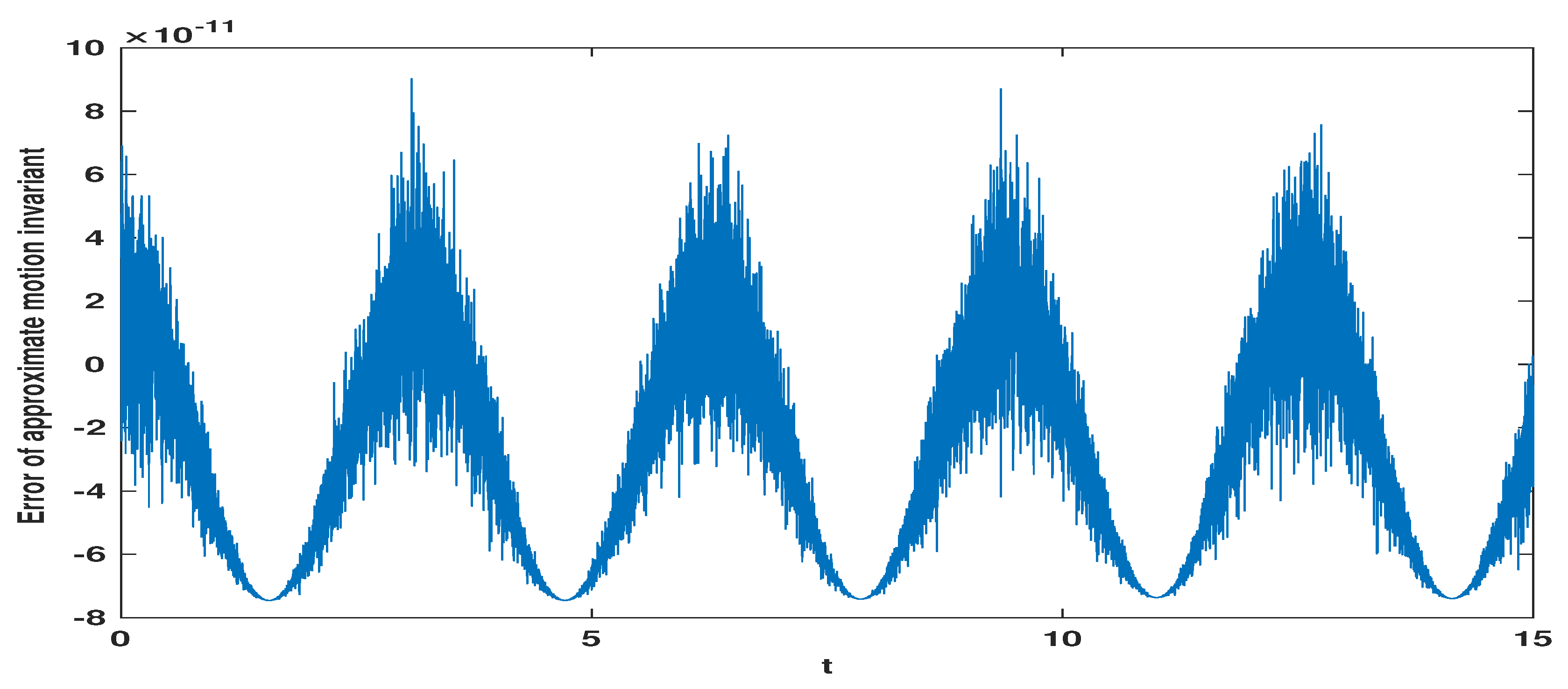
Figure 2.
Approximate motion invariant error diagram for when .
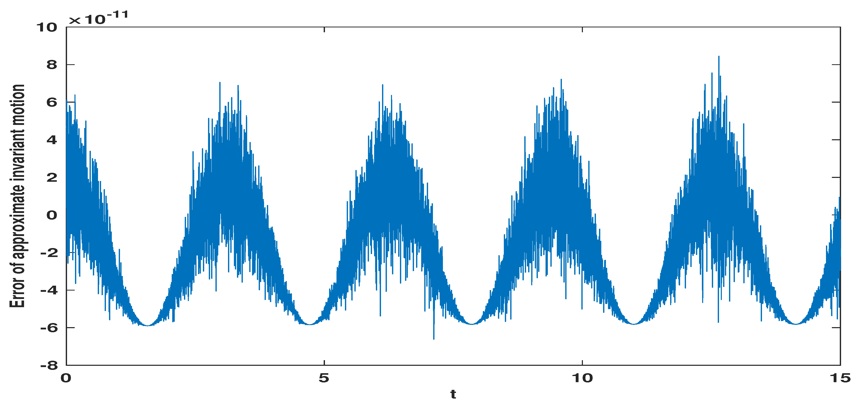
Figure 3.
Approximate motion invariant error diagram for when .
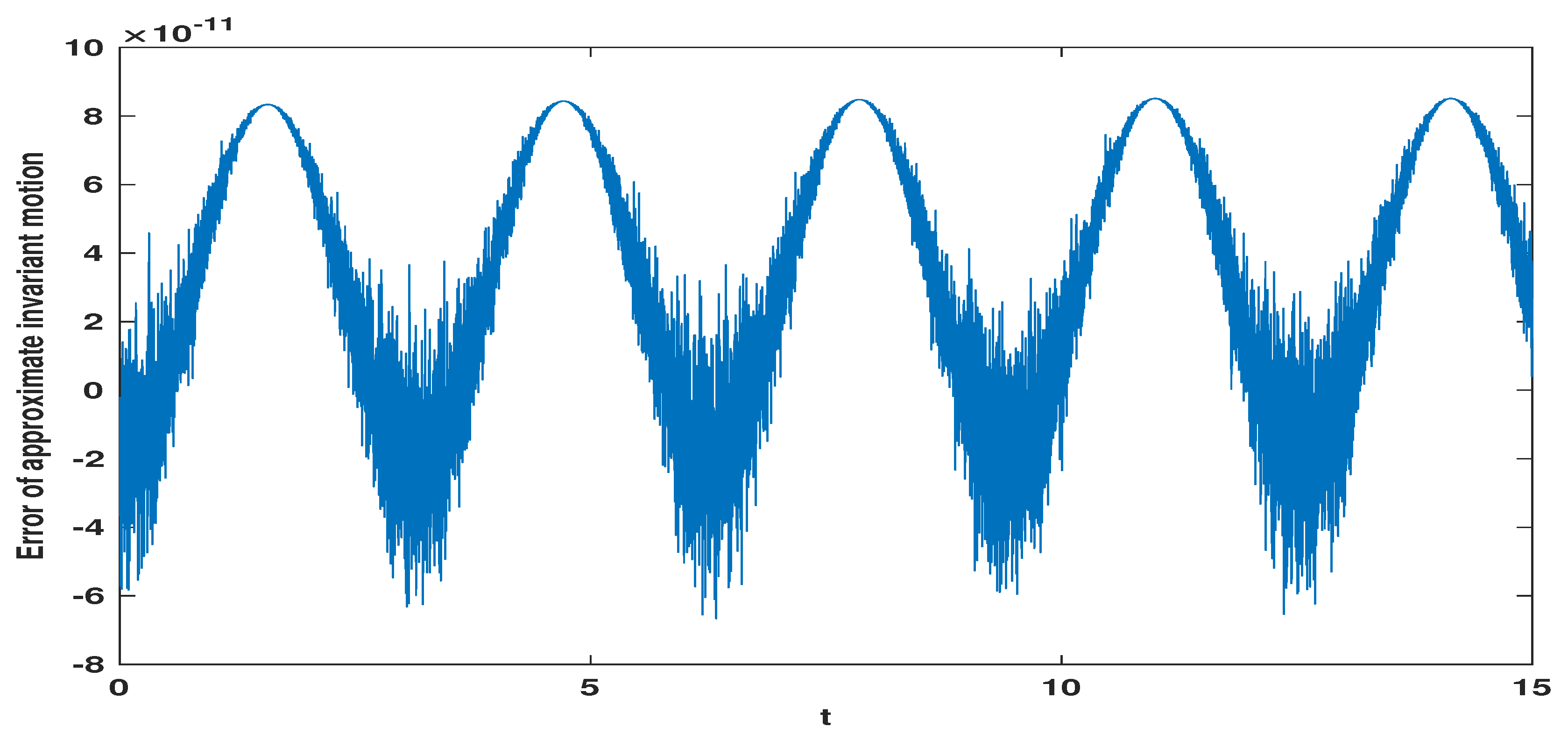
Figure 4.
error diagram for when .
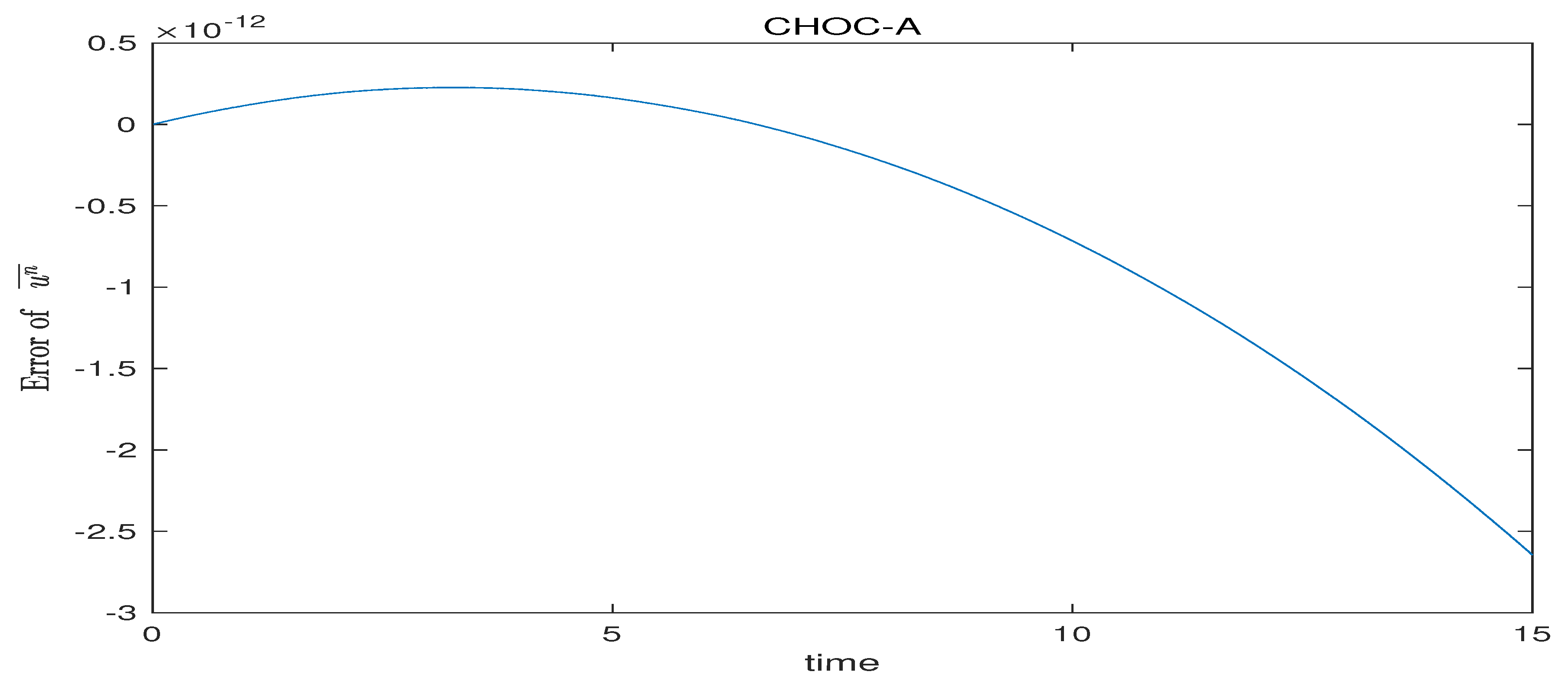
Figure 5.
error diagram for when .
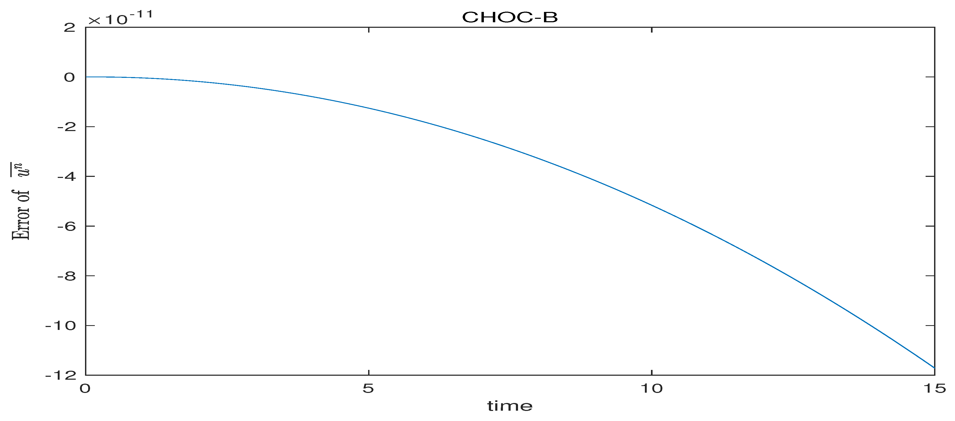
Figure 6.
error diagram for when .
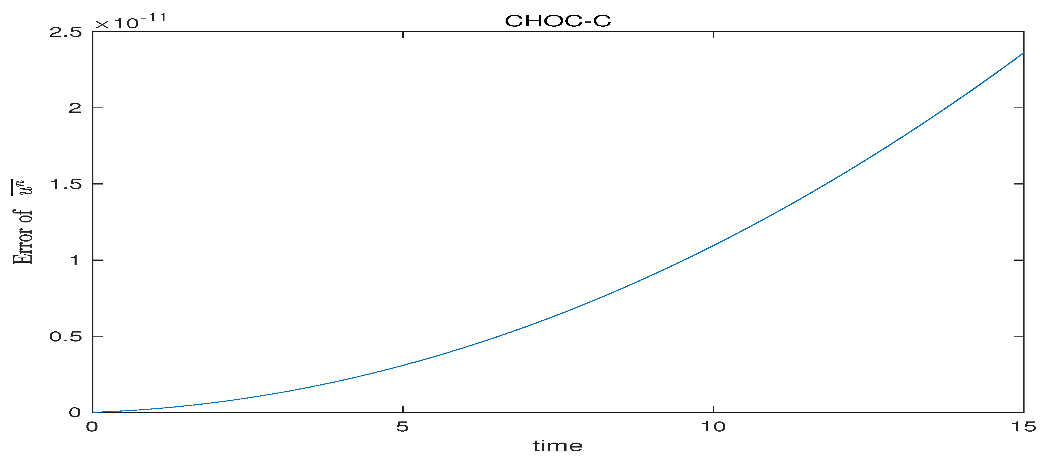
Figure 7.
When , three-dimensional waveform diagrams of the , and schemes, and three-dimensional waveform diagram of the exact solution.
Figure 7.
When , three-dimensional waveform diagrams of the , and schemes, and three-dimensional waveform diagram of the exact solution.
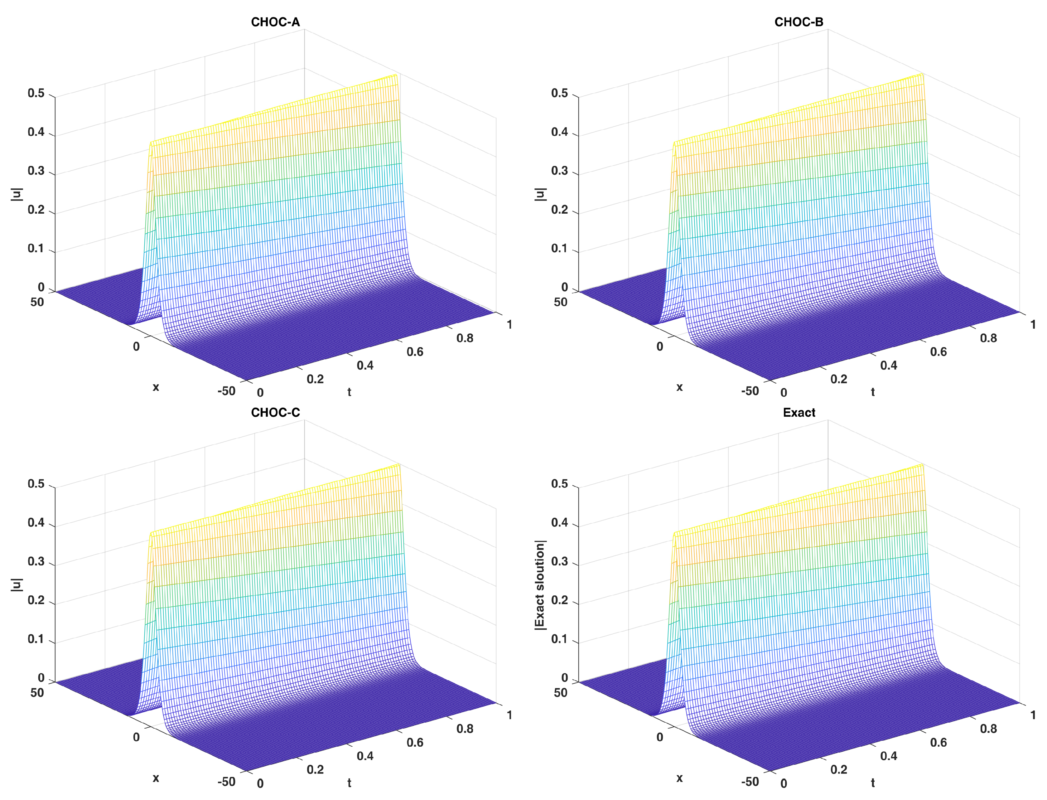
Figure 8.
when . The exact solution VS numerical solution of .
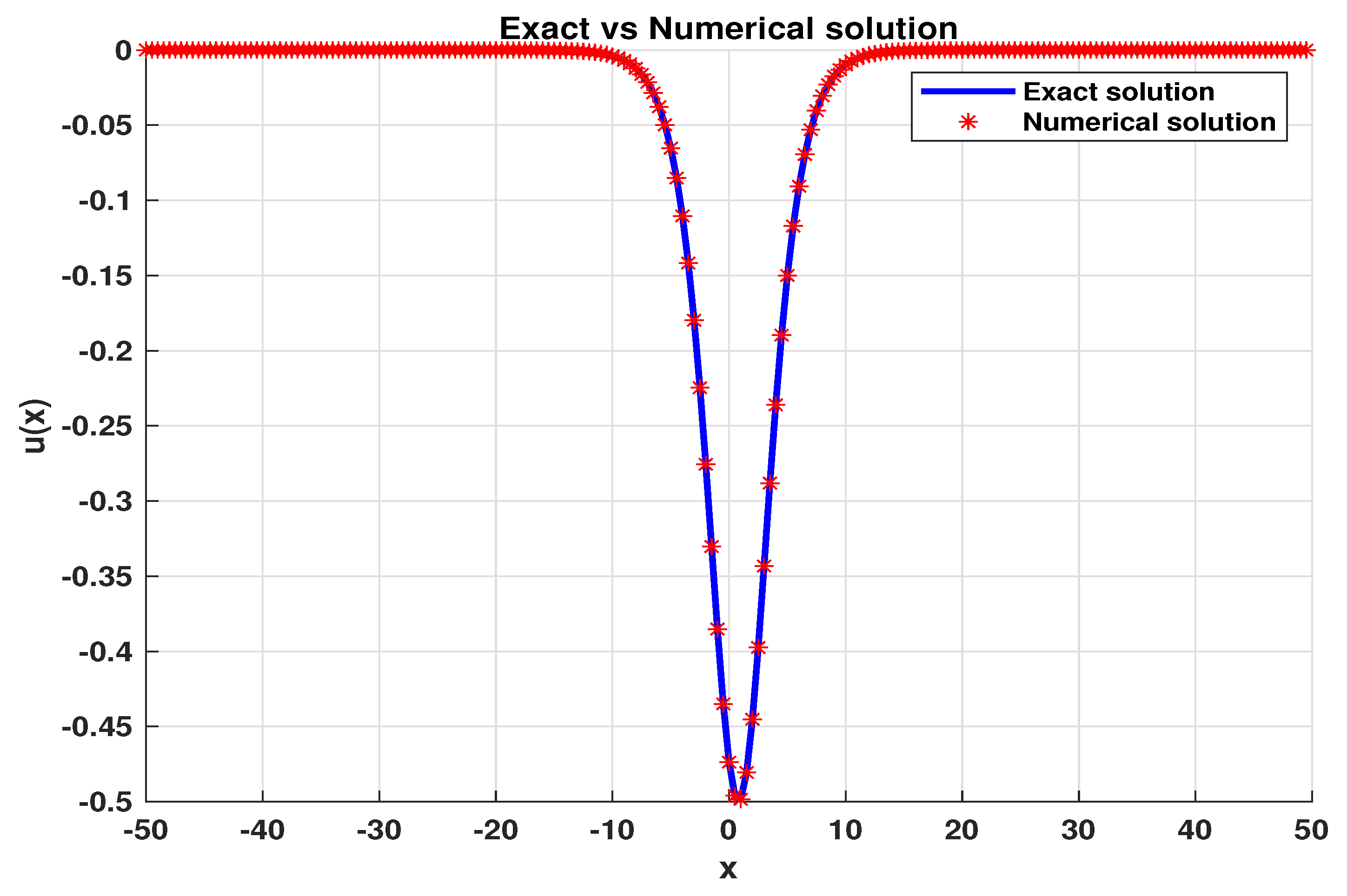
Figure 9.
when . The exact solution VS numerical solution of .
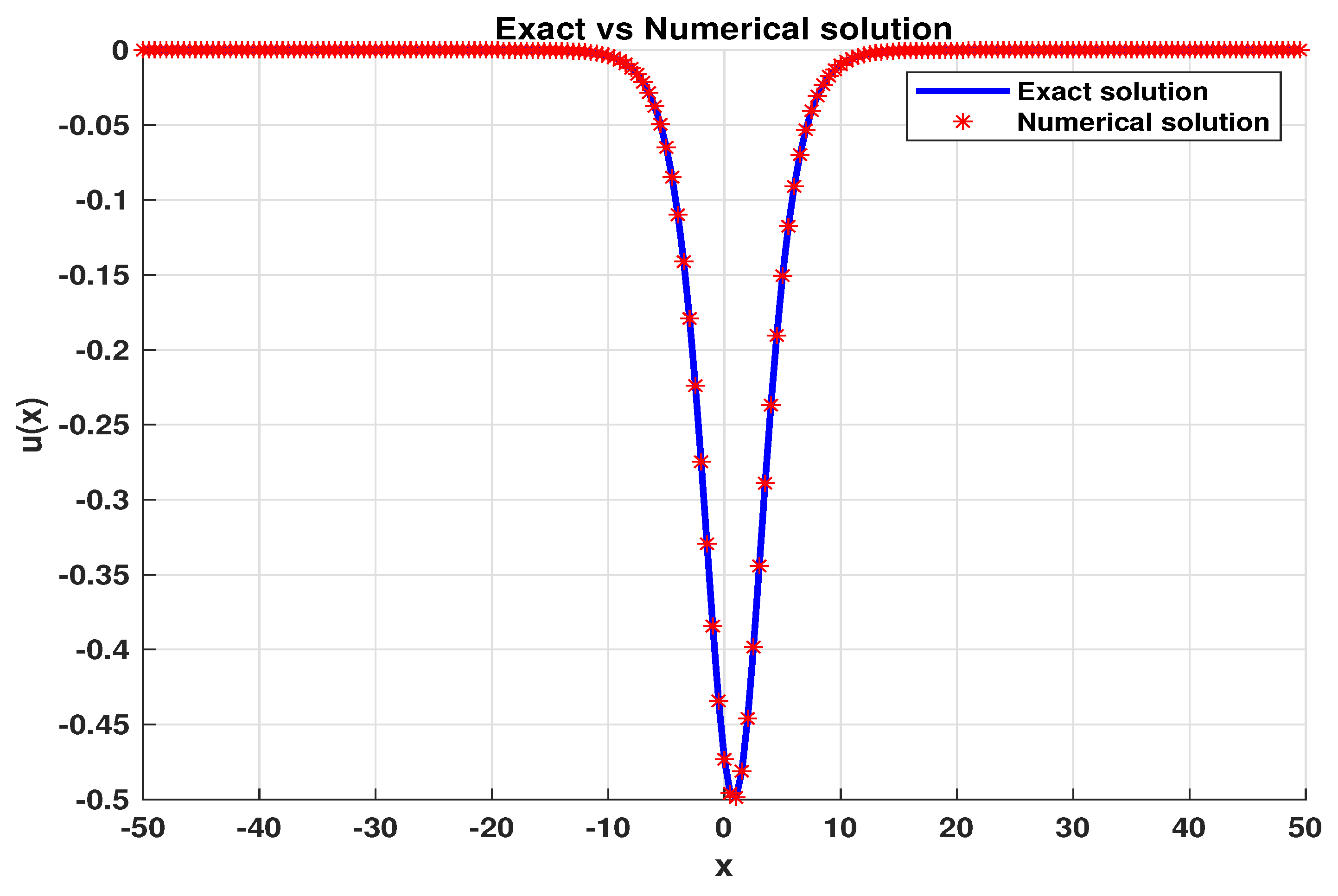
Figure 10.
when . The exact solution VS numerical solution of .
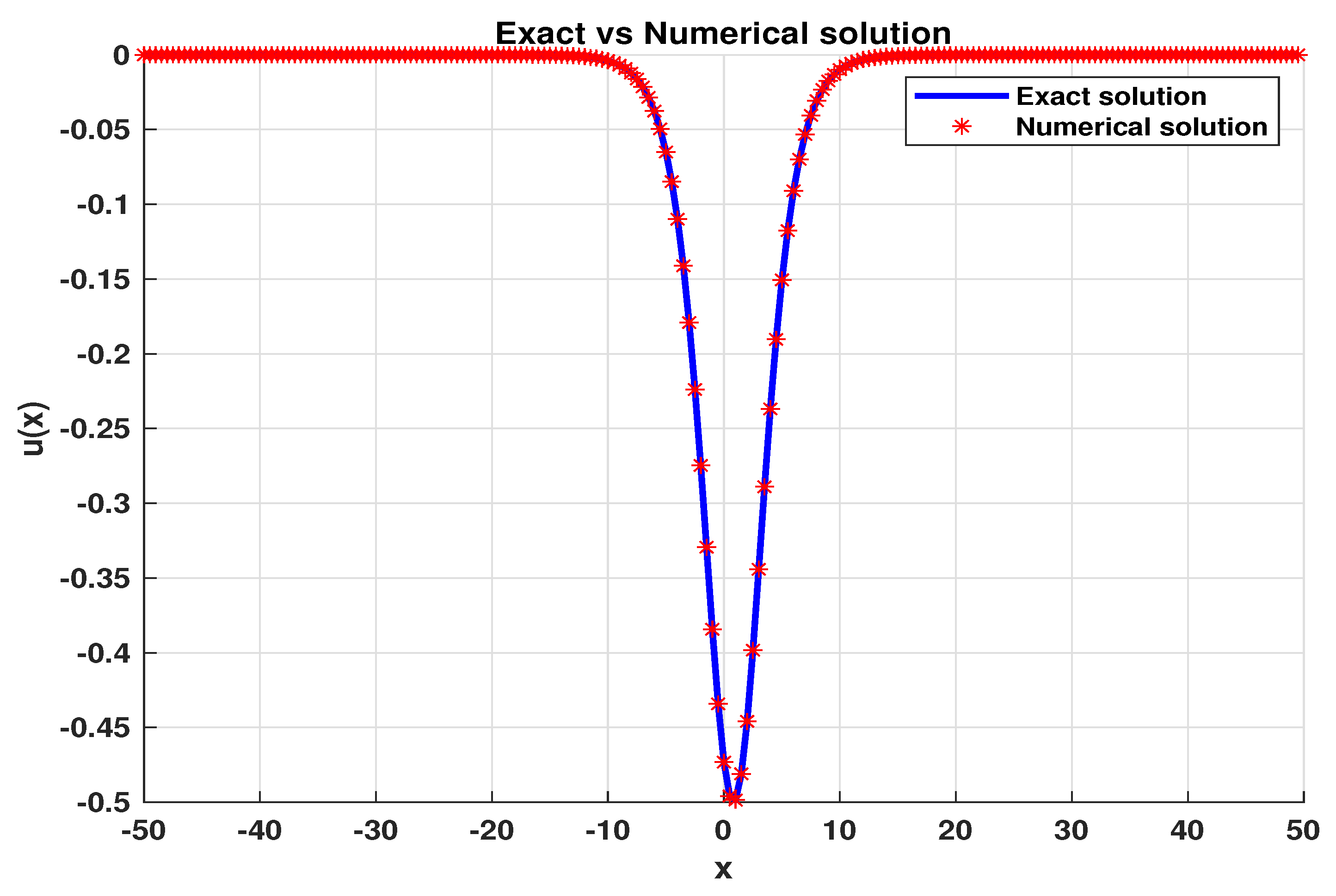

Table 1.
Taylor series of scheme(2.1).
| Term | |||||||||
|---|---|---|---|---|---|---|---|---|---|
| 0 | |||||||||
| 0 | |||||||||
| 0 | 1 | 0 | 0 | 0 | 0 | 0 | 0 | 0 | |
| 0 | 0 | ||||||||
| 0 | 0 | ||||||||
| 0 | 0 | 0 | 0 | 0 |
Table 2.
Taylor series of scheme(2.2).
| Term | |||||||||
|---|---|---|---|---|---|---|---|---|---|
| 0 | |||||||||
| 0 | |||||||||
| 0 | 0 | 1 | 0 | 0 | 0 | 0 | 0 | 0 | |
| 0 | 0 | ||||||||
| 0 | 0 | ||||||||
| 0 | 0 | 0 | 0 | 0 | 0 | 0 | 0 | ||
| 0 | 0 | 0 | 0 | 0 |
Table 3.
Taylor series of scheme(2.11).
| Term | |||||||||
|---|---|---|---|---|---|---|---|---|---|
| 0 | |||||||||
| 0 | |||||||||
| 0 | 1 | 0 | 0 | 0 | 0 | 0 | 0 | 0 | |
| 0 | 0 | ||||||||
| 0 | 0 | ||||||||
| 0 | 0 | 0 | |||||||
| 0 | 0 | 0 | |||||||
| 0 | 0 | 0 | 0 | 0 |
Table 4.
Taylor series of scheme(2.12).
| Term | |||||||||
|---|---|---|---|---|---|---|---|---|---|
| 0 | |||||||||
| 0 | |||||||||
| 0 | 0 | 1 | 0 | 0 | 0 | 0 | 0 | 0 | |
| 0 | 0 | ||||||||
| 0 | 0 | ||||||||
| 0 | 0 | 0 | |||||||
| 0 | 0 | 0 | |||||||
| 0 | 0 | 0 | 0 | 0 | 0 | 0 | 0 | ||
| 0 | 0 | 0 | 0 | 0 |
Table 5.
Taylor series of scheme(2.13).
| Term | |||||||||
|---|---|---|---|---|---|---|---|---|---|
| 0 | |||||||||
| 0 | |||||||||
| 0 | 0 | 0 | 1 | 0 | 0 | 0 | 0 | 0 | |
| 0 | 0 | ||||||||
| 0 | 0 | ||||||||
| 0 | 0 | 0 | |||||||
| 0 | 0 | 0 | |||||||
| 0 | 0 | 0 | 0 | 0 |
Table 6.
Numerical error of with .
| h | order | order | ||||
|---|---|---|---|---|---|---|
| − | − | |||||
| − | − | |||||
| − | − | |||||
Table 7.
The ratio of numerical error among different schemes of with .
| h | |||||||
|---|---|---|---|---|---|---|---|
| 10.3 | 10.5 | 8.03 | 8.2 | ||||
| 44.5 | 45.5 | 31.2 | 31.9 | ||||
| 102.1 | 102.6 | 69.4 | 69.7 | ||||
| 186.8 | 186.2 | 121 | 120.6 | ||||
| 320 | 320.6 | 178.8 | 179.2 | ||||
Table 8.
Verification of temporal convergence rate with .
| order | order | |||||
|---|---|---|---|---|---|---|
| − | − | |||||
| − | − | |||||
| − | − | |||||
Disclaimer/Publisher’s Note: The statements, opinions and data contained in all publications are solely those of the individual author(s) and contributor(s) and not of MDPI and/or the editor(s). MDPI and/or the editor(s) disclaim responsibility for any injury to people or property resulting from any ideas, methods, instructions or products referred to in the content. |
© 2024 by the authors. Licensee MDPI, Basel, Switzerland. This article is an open access article distributed under the terms and conditions of the Creative Commons Attribution (CC BY) license (https://creativecommons.org/licenses/by/4.0/).
Copyright: This open access article is published under a Creative Commons CC BY 4.0 license, which permit the free download, distribution, and reuse, provided that the author and preprint are cited in any reuse.


