Submitted:
21 May 2024
Posted:
22 May 2024
You are already at the latest version
Abstract
Real-time object detection remains a pivotal topic in the realm of computer vision. Balancing the accuracy and speed of object detectors poses a formidable challenge for both academic researchers and industry practitioners. While recent transformer-based models have showncase the prowess of the attention mechanism, delivering remarkable performance improvements over CNNs, their computational demands can hinder their effectiveness in real-time detection tasks. In this paper, we elect to use YOLOX as our robust starting point and introduce a series of effective enhancements, culminating in a new high-performance detector named YOLOAX. To further exploit the power of the attention mechanism, we devise multi-dimensional attention-based modules that activate CNNs, emphasizing the most pertinent regions and bolstering the capacity to learn the most informative image representations from feature maps. Moreover, we introduce a novel leading label assignment strategy called STA, along with a groundbreaking loss function named GEIOU Loss, to further refine our detector's performance. We provide extensive ablation studies on the COCO and PASCAL VOC 2012 detection datasets to validate our proposed methods. Remarkably, our YOLOAX is trained solely on the MS-COCO dataset from scratch, without leveraging any prior knowledge, which achieves an impressive 54.2% AP on the COCO 2017 test set while maintaining a real-time speed of 72.3 fps, surpassing YOLOX by a significant margin of 3.0% AP. Our source code and pre-trained models are openly accessible at https://github.com/KejianXu/yoloax.
Keywords:
real-time object detection
; information theory
; attention mechanism
; Region boosting
; label assignment
; information loss
1. Introduction
Object detection, especially real-time object detection, has always been a challenging topic in computer vision systems, requiring the detector to predict a bounding box with a category label as accurately and quickly as possible for each instance of interest in an image with several effective enhancements of information theory. Driven by the great success of region-based deep convolutional neural networks (R-CNNs) [1,2], the later incarnations such as Fast R-CNN, Faster R-CNN and others [3,4,5] pursuit higher accuracy while ignoring the reasoning cost on region proposals and high latency, which show poor performance to take real-time object detection tasks. With the development of object detection and information theory, research attention has been geared towards one-stage object detection. YOLO series [6,7,8,9,10] innovatively choose to trade in much faster computing speed at the cost of appropriately reduced accuracy, which achieve a better balance between high accuracy and optimal speed for real-time object detection tasks. Recently with the introduction of the anchor-free manner [11,12], the major advances with anchor-free in object detection academia like YOLOR [8] and YOLOX [9] have achieved significant performance boost over previous efforts. They focus on applying new advanced label assignment strategies [13,14,15] to automatically classify positive and negative training samples, dramatically increasing speed with guaranteed accuracy, instead of training with manually created allocation rules.
At the same time these recent years, Transformer [16] holds the best trade-off performance, a simple network framework based exclusively on multi-headed attention mechanisms for sequence transduction tasks. The follow-up efforts attempt to apply the Transformer on multiple vision tasks and begin to explore the attention mechanism in depth, which all attain SOTA results on various vision tasks. The Transformer-based models not only significantly improve the speed, but also reduce additional computational cost, which demonstrate the advantages of the attention. Despite the impressive achievements, those super large-scale models suffer from poor performance on the tasks in real-time object detection. As for conducting real-time detection tasks, we experientially argue that conventional attention-based approaches still have two main limitations: (1) Requiring enormous computing resources if the model bases solely on attention, which is not applicable for lightweight model; (2) Especially relying on strong data augmentation strategies or adequate annotations.
That’s what brings us here. Recent effort [17] show the benefit of combining transformer and convolution in series, regardless of the part in which the convolution is used. Most current mainstream object detectors are developed for GPU and use ResNet [18], CSPNet [19], or DarkNet [5] as the backbone of the network architecture. In this paper, considering the latest models may be somewhat over-optimized for anchor-free pipes, we choose YOLOX with CSPDarknet as our baseline and deliver the aforementioned advancements of information theory to YOLOX with experienced optimization. As shown in Figure 1, absorbing the essence of attention mechanism and equipped with the effective methods we proposed, we boost the YOLOX to 55.2% AP (YOLOAX) on MS-COCO 2017 test set, exceeding the counterpart YOLOX by 3.7% AP with fewer additional computational cost. We also take abundant ablation studies to validate the influence of our methods during the detector training.
2. Related Work
2.1. One-Stage Object Detectors
A conventional detector basically consists of two components, a backbone for extracting effective features, which is pre-trained on your dataset, and a head for predicting classes and regression of bounding boxes of target objects. In recent years, the most advanced two-stage detection models are mostly based on the R-CNN series, which focus on locating the object to get multi-scale anchors to ensure sufficient accuracy and recall in the first stage, and then classify the anchors to find a more precise location in the second stage. Nevertheless, as the development of one-stage models in real-time object detection, they are slow and hard to optimize comparing to other SOTA one-stage real-time detectors. The most representative one-stage object detection frameworks are mainly based on YOLO series, SSD [20] and RetinaNet [21], which can achieve much faster detection speeds at the cost of slightly reduced accuracy. To get faster speed without increasing additional inference cost, the one-stage object detectors with anchor-free manner are developed. The models of this sort are FCOS series [22,23]. Currently, the most representative real-time object detectors usually require a stronger and faster network architecture as the backbone like ResNet, CSPNet, DarkNet, etc. and may integrate various layers or more effective methods to further optimize the model. Some researchers put their attention on designing a new whole model or a new powerful backbone for object detection. By contrast, some efforts aim to explore more effective approaches for detection. Lin et al. (2017) [2] proposed a new mechanism called Feature Pyramid Network (FPN), which can learn informative image representations by fusing feature maps collecting from different shapes. Obviously shown in previous researches [9,14,21,24], a more robust and powerful loss function and an advanced label assignment strategy are both play an important role for models achieving high performance. One of the important contributions of this work is designing some new advanced learning methods associated with the mentioned above for optimizing the model.
2.2. Attention Mechanism
As for human visual system, one crucial property is that humans can selectively focus on salient parts through a sequence of partial glimpses when staying in a whole scene, which is largely attributable to attention mechanisms. Recently, the significance of attention in deep learning has been studied extensively in previous works [25,26]. Especially the proposal of Transformer took the research of attention to a new level. The follow-up models achieved impressive performance not only on multiple computer vision tasks but also on nature language processing tasks, showing the power of attention mechanism to tell where should focus and improve the image representation of interests. To further explore the potential of attention, in recent years, Hu et al. (2019) [27] proposed SENet, which is composed of two core parts, a squeeze module which is used to model channel dependencies of feature maps and learn the corresponding information between channels, and an excitation module which is used to adaptively learn the feature of interest based on channel-wise attention and weight the representations of different channels. Then Wang et al. (2020) [28] propose an enhanced network structure called ECANet, applying a local cross-channel engagement method for avoiding dimensional reduction, which result in excellence performance without increasing the model’s computational complexity. Additionally, the BAM and CBAM [29,30], which infer the attention weights along both spatial and channel dimensions in turn, can be seamlessly integrated into any deep learning architectures and trained in an end-to-end manner with the basic CNN to perform adaptive feature optimization. Based on these studies, one of the main goals of our work is to fully utilize the role of attention mechanism. In this paper, two new modules based on attention are proposed, to activate the model to focus more on the more useful and interesting regions and capture the most important image representations based on spatial attention, which can significantly boost the ability for global image representations learning.
3. Architecture
We opt for YOLOX with CSPDarknet as a strong baseline and have substantially modified the structure of YOLOX, forming a new high-performance detector YOLOAX. In the subsequent part, we will step-by-step introduce the entire architecture designs in YOLOAX. The overview of YOLOAX architecture is illustrated in Figure 2.
3.1. Cross-Stage Partial Attention Module
To exploit the potential of attention mechanism, we present a cross-stage partial attention module called CSPAM to serve as the base module of our backbone, as illustrated in Figure 3.
Given a feature map as input, CSPAM is a computational unit which can map the input to the output . The representations of the input will be initially learned through a channel self-attention module (CSAM) we proposed, which can activate the model to selectively inhibit less useful features and emphasize informative ones by learning to use global information. The CSAM can be embedded in any CNN modules to effectively enhance the ability of learning the representations useful for detectors. The whole architecture design of CSAM is illustrated in Figure 4 and the results of assessing the power of proposed CSPAM are demonstrated in section 4.2.
Considering the problem that each learned filters with a local receptive field has difficulty exploiting contextual information outside that region, we first decide to use global average pooling operation to squeeze global information into each channel space and refer to each channel output as . The statistic Z is formally generated by shrinking the spatial dimensions H × W of , as defined:
Subsequently, to analyze the mechanisms of each channel and focus on the most discriminative features, we utilize 1×1 base convolutional operation twice in succession. It’s our view that each information value the model learned is almost compressed from 2D feature maps of each channel and can be thought of as getting a global receptive field in a way of information theory. The output is denoted as S, which is calculated by:
where represents a standard 2d convolutional layer with batch normalization operation and SiLU.
To mitigate negative activations and normalize , as for non-linear activation function, instead of ReLU, our work opt for the smoother activation function SiLU, which outperforms ReLU especially when training deep learning models and processing with more complex information feature maps. By utilizing the as normalized weighting factors or scalar, the two dimensions of height and width of the input are rescaled with in each channel to obtain the final feature map U, which adaptively highlight the more informative representation of the information feature map:
⨂ represents channel-wise multiplication.
Since the outstanding performance of residual learning framework, our proposed CSPAM adopts the bottleneck architecture of the CSPDarknet to mitigate the gradient disappearance, and optimize the network degradation problems and the training difficulties. For the main considerations that reducing the computational density and the amount of hyperparameters, the channels of input will first be expanded to twice its original size after a 1×1 base convolutional operation , and then the channels will be split in half, which one less convolutional operation can be performed comparing to the previous module. The output will be processed separately on both channels, one is successively convolved using a 3×3 base convolutional kernel with a step size of two through three bottleneck structures, and its channels is divided into two halves each time, while the other without any operations. Information data from one of the channels of the feature map is retained for stacking at the end after each one pass through a bottleneck structure, which can be regarded as a dense residual structure or information extractor.
After initial feature extraction in multiple CSPAMs, the output of the penultimate and the third CSPAM from different shapes is saved and fed into the FPN structure for enhanced feature extraction. We decide to keep the original FPN structure with the fewest possible modifications and design a pooling module, which is based on spatial attention, in order to extract deterministic feature information from the output of the last CSPAM. More details please refer to the next section.
3.2. Spatial Feature Pooling Module
It is crucial for model to enhance the capability to capture spatial representations and information of features, therefore we propose a Spatial Feature Pooling Module called SFPM, showing in Figure 5, to replace the SPPBottleneck of CSPDarknet. The input from the last CSPAM is set to and the will first be fed into g and c separately for different feature extraction. g and c denote feature extractors. In c, to preserve original features as much as possible, it just contains a layer of 1×1 base convolution, but reduce the channels of the input map to half the original number, which tentatively generates the statistics . In g, it contains a layer of 3×3 base convolution, a layer of 1×1 base convolution, and a layer using global pooling. To explore the importance of each channel, after initial extraction in the first two layers, we can get a feature tensor denoted . Subsequently, we separately utilize global max pooling operations on the . Specifically, for learning useful spatial information, in global pooling layer, three parallel pooling kernels of different sizes will be adopted to extract feature representations of different shapes, and the output can be got:
Then we perform channel-wise dimensional concat on the and aggregate them together with the following equation:
Finally, after performing dimensional concat on with , and a 1×1 base convolutional operation , we obtain the most informative output :
The output, enriched with information from various sources, will be fed into the FPN structure. Here, it undergoes a process of fusion with other features, each possessing distinct shapes and carrying unique informational content. This integration is crucial in information theory, as it allows for the aggregation of diverse data streams, enriching the overall informational value. By extracting and combining these features, the FPN structure generates three enhanced features that capture a more comprehensive representation of the input data. These enhanced features, which embody the essence of the original information while also incorporating new perspectives, are ultimately utilized for prediction, leveraging the power of information theory to achieve accurate and insightful outcomes.
3.3. Anchor-Free
There are some known conflicts between classification and regression tasks when models using for object detection with original anchor-based detectors. In the aspects of the overall inference complexity and latency, anchor mechanism may become the potential bottleneck, especially moving large amount of predictions for each image between devices on serval special AI systems. Following the exploration of DenseBox [31] and YOLO, the performance of Anchor-free detectors has been widely acknowledged in the past five years, which can attain the same AP on object detection as anchor-based one while reducing the number of parameters.
Based on Anchor-free manner of YOLOX, we propose a new decoupled head, as shown in Figure 6, without the branch for IoU to lighten the model in terms of both speed and size. Firstly, we can obtain three enhanced features of different shapes via the FPN structure and define the input feature maps as . Then the input are separately processed through two parallel convolutional lines for the prediction of classification (Cls) and regression (Reg), which is composed of two layers of 3×3 base convolution and two 1×1 convolutional layers. We take tr to be an operator to denote the above series of convolutional operations of each line, to get the final tensor for the branches to compute loss:
We still opt for BCE Loss for training classification branch, but we propose a new information loss function Generalized Efficient IOU Loss called GEIOU Loss for regression branch because we infer the original use of IOU Loss may harm the performance. Compared to previous Losses, GEIOU introduces Generalized Focal Loss [24] to achieves the great balance between easy and hard samples in the regression stage, and address the problem of learning distributed and qualified representation for dense detection.
In GEIOU, given the box of prediction and the ground truth box , we divide the calculation of Reg loss into two parts: the first part uses EIOU Loss [21] to calculate the IOU between and ; the latter part uses GFL to accurately locate box in arbitrary distribution and depict the flexible distribution in real data. The specific formulation of EIOU Loss can be defined as follows:
where and mean the center points of each B and B^gt. , and , indicates the height and width of and , respectively. and represent the height and width of the smallest outer box that covers both boxes.
Considering the problem that, if the number of high-quality anchors is much less than poor samples’s with large regression errors, it may produce large gradient to affect the training phase when in a bounding box regression task. To tackle the problem, we reweight the EIOU Loss by using the value of GFL and get 𝓛GEIOU as follows:
where the specific formulation and derivation of GFL can be found in [24], and β can be seen as a controlling parameter to inhibit outliers. We also take ablation studies and observe significant improvements over counterparts trying other IOU Loss. More details are shown in section 4.2.
3.4. Simple Task Assigner
Due to the fact that advanced label assignments have become an important progress for object detection, we opt for SimOTA [9] as our start point and optimize it a bit. And considering the excellence of the dynamic label assignments, we choose to combine it with TaskAlignedAssigner [32] in a weighted way, and propose a simple task assigner named STA for optimal transport problem.
For reducing the cost between ground truth box and prediction , we first add a new element, which is defined as E and denotes the samples that are excluded in the intersection part of and , to the cost function in SimOTA and use a coefficient μ to control the degree of scaling of the E. The new cost we proposed is calculated as:
where 𝓛cls and 𝓛reg are Cls loss and Reg loss between and . The and are both balancing coefficients, and the is a controlling coefficient, an extremely large constant which we take the value of 10^5, to force the detector to prefer samples within the intersection for matching in the process of minimizing cost.
Cij = α𝓛cls + λ𝓛reg + μE,
Then inspired by the assigning strategy in TaskAlignedAssigner, which select positive samples based on the scores weighted by the Cls and Reg scores, we modify the as the follow equation:
For each , the degree of alignment can be measured by multiplying the two weighted loss, and finally the top k prediction with the least inference cost are selected as its positive samples. As shown in section 4.2, the STA show its power, which raises the performance of our detector from 50.7% AP to 51.3% AP.
4. Experiments
We perform sufficient experiments for our proposed object detection methods on COCO dataset [33] and PASCAL VOC test set [34]. All models of object detection in our experiments were not pre-trained, which were just trained from scratch. We choose 2017 train set to train our detector and use 2017 val dataset to validate and choose the optimal hyperparameter combinations. The high performance of our detector YOLOAX on the 2017 test dataset is shown at last. Experimental settings and detailed training parameter setup are described in the following section.
4.1. Experimental Settings
We opt for YOLOX with CSPDarknet as our baseline and design a basic model called YOLOAX for normal GPU. All the models and our proposed methods are trained on two parallel V100 GPU. Unless otherwise specified, our methods are all trained and tested at 640 × 640 resolution on the COCO dataset. Only the category labels of the images are used as annotations without any prior information.
To optimize our model, we experientially choose the SGD with a momentum of 0.937 as optimizer and set the total training process to 300 epochs. After several experimental comparisons, we initially set the learning rate to 1e-2 with warmup during the early processes of training, while reducing to 1/100 of last in a way of cosine annealing for every 30 epochs. And we employ a weight decay of 5e-4 and set the mini-batch size to 16. As for strong data augmentation strategies, we adopt Mix-up and Mosaic implementations during our training but stop it in the last 30 epochs for the model’s better performance. Nevertheless, during the training process, we found the benefit that suitable data augmentation strategies bring to model varies across different size of models. Therefore, when training small models such as YOLOAX-S, we weaken the Mosaic augmentation and remove the Mix-up. Such a modification, as demonstrated in Table 1, boost the performance of YOLOAX-S from 44.8% AP to 45.1% AP.
4.2. Ablation Studies
Proposed Modules In order to ensure a fair comparison, we opted to utilize the identical backbone as YOLOX, incorporating CSPDarknet along with the FPN structure. Recognizing the immense potential of the attention mechanism, we introduced a novel cross-stage partial attention module, christened CSPAM, that leverages channel attention. We integrated our CSPAM into the YOLOX-S model to evaluate its performance, followed by conducting ablation studies on the MS-COCO and PASCAL VOC datasets for comparative analysis. Figure 7 presents the compelling results of the attention visualization from superficial layers, clearly demonstrating that the CSPAM outperforms the baseline, bolstering the model's ability to learn meaningful image representations. The findings in Table 2 and Table 3 further corroborate the effectiveness of our CSPAM. On the MS-COCO dataset, the detector's AP rose from 40.5% to 40.8%, while on the PASCAL VOC dataset, it increased from 81.5% to 82.6%. These improvements were achieved while reducing the number of parameters by approximately 13%. This reduction in parameters not only enhances efficiency but also underscores the efficiency of our CSPAM in extracting critical features.
Proposed Optimization Methods In recent years, advanced label assignment is one of the core progresses of real-time object detection. For further optimize our model, based on the previous study SimOTA and TaskAlignedAssigner, we thus design a simple task assigner named STA. Comparing to SimOTA, we take the issue of the degree of scaling into account and set an extremely large constant to force the detector to prefer samples within the intersection for matching in the process of minimizing cost, which increase the speed of inference and accuracy of assigning true samples. It is obviously shown in Table 4 that our STA raises the performance of our detector from 51.0% AP to 52.3% AP on MS COCO. We also conduct ablation studies on other detectors to test the performance when applying STA, where STA achieves performance improvements against all the corresponding counterparts, especially about ~1.7% to ~3.1% AP improvements basing on FCOS.
Proposed Loss for Yolo_head Recently a trend for models in real-time object detection is to introduce two individual branch to take the prediction of localization and estimate the quality of regression, which the quality of prediction facilitates the classification ability to improve detector performance. Therefore, a more robust information loss is another important factor for real-time object detection process. Since we argue the Obj. branch plays a very minor role. Different from the manner of YOLOX, we only keep the branch for classification and regression with removing the Obj. branch, which can also increase the speed when computing loss. Normally, we still use BCE Loss for classification branch when training our detector. In terms of regression branch, we propose a Generalized Efficient IOU Loss called GEIOU, effectively reducing the regression loss of our object detector. To access the quality of our information loss, we select the YOLOX-M as our baseline and take some ablation studies on COCO dataset and PASCAL VOC dataset by trying different IOU Loss for the prediction of regression. In Table 5, it’s clear that the significant improvements over other counterparts can be observed based on our proposed method on PASCAL VOC, higher than EIOU and baseline by 0.4% AP and by 2.8% AP, respectively. And on COCO, there are also small performance gains on the MS-COCO dataset.
Backbones We adhere to the scaling rule outlined by YOLOX in order to develop the diverse models that comprise the YOLOAX series, which includes models designated as S, M, L, and X. In our rigorous testing process, we subjected all models to an image scale of 640 pixels and a batch size of 1, utilizing two parallel V100 GPUs. The results, as presented in Table 6, are nothing short of impressive. Our models demonstrate a consistent and significant improvement in performance compared to the YOLOX series. Specifically, we observe an increase in average precision (AP) ranging from approximately 5.0% to 3.0% on the MS COCO dataset, without any undue increase in inference cost. This remarkable performance enhancement in Figure 8 validates the effectiveness of our approach in designing and scaling the YOLOAX series of models.
4.3. Comparison with State-of-the-Arts
There is a tradition to show the state-of-the-art comparing table as in Table 7. Comparing to other SOTA models in real-time object detection for normal GPUs, our proposed detector comprehensively achieves the best accuracy-speed trade-off. Our method is on average about 25 fps faster and 4.1% more accurate on AP between our proposed YOLOAX series and YOLOX series, especially our YOLOAX-X is 24 fps faster than the YOLOX-X, boosting by about 41%. In addition, YOLOAX-M get 52.3% AP at 105 fps frame rate, while PPYOLOE-L has only 78 fps frame rate with the same AP, reducing about 34%. Our proposed YOLOAX series favor lighter weight, especially YOLOAX-M is 57% less than the YOLOv7 in terms of parameter usage, which is suitable for real-time detection. Keeping in mind that, as for computation and parameters, YOLOAX-X reduces 12% of computational parameters compared to YOLOX-X, but improves AP by 3.7%. And the visualization results of object detection in Figure 9 clearly demonstrates that YOLOAX outperforms YOLOX in terms of quantity and quality of object detection.
5. Conclusion
In this paper, we introduce several significant enhancements of information theory to the YOLOX framework, culminating in a high-performance object detector YOLOAX. Our proposed YOLOAX series excels over the YOLOX series in crucial aspects such as speed, accuracy, and model parameter efficiency. Leveraging the innovative modules we propose, namely CSPAM and SFPM, YOLOAX demonstrates an enhanced capacity to capture the most pertinent image representations compared to YOLOX. Additionally, by incorporating an advanced label assignment strategy called STA and an optimized information loss function GEIOU, YOLOAX achieves an optimal balance between accuracy and speed, surpassing other state-of-the-art real-time detectors. Notably, our YOLOAX-X model attains an impressive 55.2% AP on the MS-COCO dataset, maintaining a real-time speed of 82.4 fps, thereby surpassing YOLOX-X by a notable margin of 3.7% AP.
Author Contributions
Conceptualization, K.X.; methodology, K.X.; validation, K.X.; formal analysis, K.X., Z.X. and J.C.; investigation, K.X.; resources, K.X.; data curation, K.X.; writing—original draft preparation, K.X. and Z.X.; writing—review and editing, K.X., Z.X., Y.N. and J.C.; visualization, K.X.; supervision, Z.X., Y.N. and J.C.; project administration, J.C. All authors have read and agreed to the published version of the manuscript.
Funding
This work was funded by the Guangxi Science and Technology Development Project (AB23026315; AB21220011), and the Guilin Science and Technology Plan Project (20210220).
Institutional Review Board Statement
Not applicable.
Informed Consent Statement
Not applicable.
Data Availability Statement
Data are contained within the article.
Conflicts of Interest
The authors declare no conflict of interest.
References
- Girshick, R.; Donahue, J.; Darrell, T.; et al. Rich feature hierarchies for accurate object detection and semantic segmentation. In Proceedings of the IEEE conference on computer vision and pattern recognition; 2014; pp. 580–587. [Google Scholar]
- Lin, T.Y.; Dollár, P.; Girshick, R.; et al. Feature pyramid networks for object detection. In Proceedings of the IEEE conference on computer vision and pattern recognition; 2017; pp. 2117–2125. [Google Scholar]
- Girshick, R.; Donahue, J.; Darrell, T.; et al. Rich feature hierarchies for accurate object detection and semantic segmentation. In Proceedings of the IEEE Conference on Computer Vision and Pattern Recognition, Mandi, India, 16–19 December 2014; pp. 580–587. [Google Scholar]
- Ren, S.; He, K.; Girshick, R.; Sun, J. Faster R-CNN: Towards Real-Time Object Detection with Region Proposal Networks. IEEE Transactions on Pattern Analysis and Machine Intelligence 2016, 39, 1137–1149. [Google Scholar] [CrossRef] [PubMed]
- He, K.; Gkioxari, G.; Dollár, P.; et al. Mask r-cnn. In Proceedings of the IEEE international conference on computer vision; 2017; pp. 2961–2969. [Google Scholar]
- Xu, S.; Wang, X.; Lv, W.; et al. PP-YOLOE: An evolved version of YOLO. arXiv 2022, arXiv:2203.16250. [Google Scholar]
- glenn jocher et al. yolov5. 2021. Available online: https://github.com/ ultralytics/yolov5 (accessed on 18 May 2020).
- Wang, C.Y.; Yeh, I.H.; Liao, H.Y.M. You only learn one representation: Unified network for multiple tasks. arXiv 2021, arXiv:2105.04206. [Google Scholar]
- Ge, Z.; Liu, S.; Wang, F.; et al. Yolox: Exceeding yolo series in 2021. arXiv 2021, arXiv:2107.08430. [Google Scholar]
- Wang, C.Y.; Bochkovskiy, A.; Liao, H.Y.M. YOLOv7: Trainable bag-of-freebies sets new state-of-the-art for real-time object detectors. In Proceedings of the IEEE/CVF Conference on Computer Vision and Pattern Recognition; 2023; pp. 7464–7475. [Google Scholar]
- Huang, L.; Yang, Y.; Deng, Y.; et al. Densebox: Unifying landmark localization with end to end object detection. arXiv 2015, arXiv:1509.04874. [Google Scholar]
- Girshick, R.; Donahue, J.; Darrell, T.; et al. Rich feature hierarchies for accurate object detection and semantic segmentation. In Proceedings of the IEEE conference on computer vision and pattern recognition; 2014; pp. 580–587. [Google Scholar]
- Zhang, S.; Chi, C.; Yao, Y.; et al. Bridging the gap between anchor-based and anchor-free detection via adaptive training sample selection. In Proceedings of the IEEE/CVF conference on computer vision and pattern recognition; 2020; pp. 9759–9768. [Google Scholar]
- Zhang, X.; Wan, F.; Liu, C.; et al. Freeanchor: Learning to match anchors for visual object detection. Advances in neural information processing systems 2019, 32. [Google Scholar]
- Ma, Y.; Liu, S.; Li, Z.; et al. Iqdet: Instance-wise quality distribution sampling for object detection. In Proceedings of the IEEE/CVF Conference on Computer Vision and Pattern Recognition; 2021; pp. 1717–1725. [Google Scholar]
- Vaswani, A.; Shazeer, N.; Parmar, N.; Uszkoreit, J.; Jones, L.; Gomez, A.N.; Kaiser, L.; Polosukhin, I. Attention is all you need. In: NeurIPS (2017).
- Guo, J.; Han, K.; Wu, H.; et al. Cmt: Convolutional neural networks meet vision transformers. In Proceedings of the IEEE/CVF Conference on Computer Vision and Pattern Recognition; 2022; pp. 12175–12185. [Google Scholar]
- He, K.; Zhang, X.; Ren, S.; et al. Deep residual learning for image recognition. In Proceedings of the IEEE conference on computer vision and pattern recognition; 2016; pp. 770–778. [Google Scholar]
- Wang, C.Y.; Liao HY, M.; Wu, Y.H.; et al. CSPNet: A new backbone that can enhance learning capability of CNN. In Proceedings of the IEEE/CVF conference on computer vision and pattern recognition workshops; 2020; pp. 390–391. [Google Scholar]
- Liu, W.; Anguelov, D.; Erhan, D.; et al. Ssd: Single shot multibox detector. In Proceedings of the Computer Vision–ECCV 2016: 14th European Conference, Proceedings, Part I 14. Amsterdam, The Netherlands, 11–14 October 2016; Springer International Publishing, 2016; pp. 21–37. [Google Scholar]
- Zhang, Y.F.; Ren, W.; Zhang, Z.; et al. Focal and efficient IOU loss for accurate bounding box regression. Neurocomputing 2022, 506, 146–157. [Google Scholar] [CrossRef]
- Tian, Z.; Shen, C.; Chen, H.; et al. Fcos: Fully convolutional one-stage object detection. In Proceedings of the IEEE/CVF interna-tional conference on computer vision; 2019; pp. 9627–9636. [Google Scholar]
- Tian, Z.; Shen, C.; Chen, H.; et al. FCOS: A simple and strong anchor-free object detector. IEEE Transactions on Pattern Analysis and Machine Intelligence 2020, 44, 1922–1933. [Google Scholar] [CrossRef] [PubMed]
- Li, X.; Wang, W.; Wu, L.; et al. Generalized focal loss: Learning qualified and distributed bounding boxes for dense object detection. Advances in Neural Information Processing Systems 2020, 33, 21002–21012. [Google Scholar]
- Guo, M.H.; Xu, T.X.; Liu, J.J.; et al. Attention mechanisms in computer vision: A survey. Computational visual media 2022, 8, 331–368. [Google Scholar] [CrossRef]
- Choromanski, K.; Likhosherstov, V.; Dohan, D.; et al. Rethinking attention with performers. arXiv 2020, arXiv:2009.14794. [Google Scholar]
- Hu, J.; Shen, L.; Sun, G. Squeeze-and-excitation networks. In Proceedings of the IEEE conference on computer vision and pattern recognition; 2018; pp. 7132–7141. [Google Scholar]
- Wang, Q.; Wu, B.; Zhu, P.; et al. ECA-Net: Efficient channel attention for deep convolutional neural networks. In Proceedings of the IEEE/CVF conference on computer vision and pattern recognition; 2020; pp. 11534–11542. [Google Scholar]
- Park, J.; Woo, S.; Lee, J.Y.; et al. Bam: Bottleneck attention module. arXiv 2018, arXiv:1807.06514. [Google Scholar]
- Woo, S.; Park, J.; Lee, J.Y.; et al. Cbam: Convolutional block attention module. In Proceedings of the European conference on computer vision (ECCV); 2018; pp. 3–19. [Google Scholar]
- Huang, L.; Yang, Y.; Deng, Y.; et al. Densebox: Unifying landmark localization with end to end object detection. arXiv 2015, arXiv:1509.04874. [Google Scholar]
- Feng, C.; Zhong, Y.; Gao, Y.; et al. Tood: Task-aligned one-stage object detection. In Proceedings of the 2021 IEEE/CVF International Conference on Computer Vision (ICCV). IEEE Computer Society; 2021; pp. 3490–3499. [Google Scholar]
- Lin, T.Y.; Maire, M.; Belongie, S.; Bourdev, L.; Girshick, R.; Hays, J.; Perona, P.; Ramanan, D.; Zitnick, C.L.; Doll’ar, P. Microsoft coco: Common objects in context. In: ECCV (2014).
- Everingham, M.; Gool, L.; Williams, C.K.; Winn, J.; Zisserman, A. The pascal visual object classes (voc) challenge. IJCV (2010).
- Carion, N.; Massa, F.; Synnaeve, G.; Usunier, N.; Kirillov, A.; Zagoruyko, S. End-to-end object detection with transformers. In Proceedings of the European Conference on Computer Vision (ECCV); 2020; pp. 213–229. [Google Scholar]
Figure 1.
Comparison of our proposed YOLOAX and other real-time object detectors, our methods achieve the best accuracy-speed trade-off.
Figure 1.
Comparison of our proposed YOLOAX and other real-time object detectors, our methods achieve the best accuracy-speed trade-off.
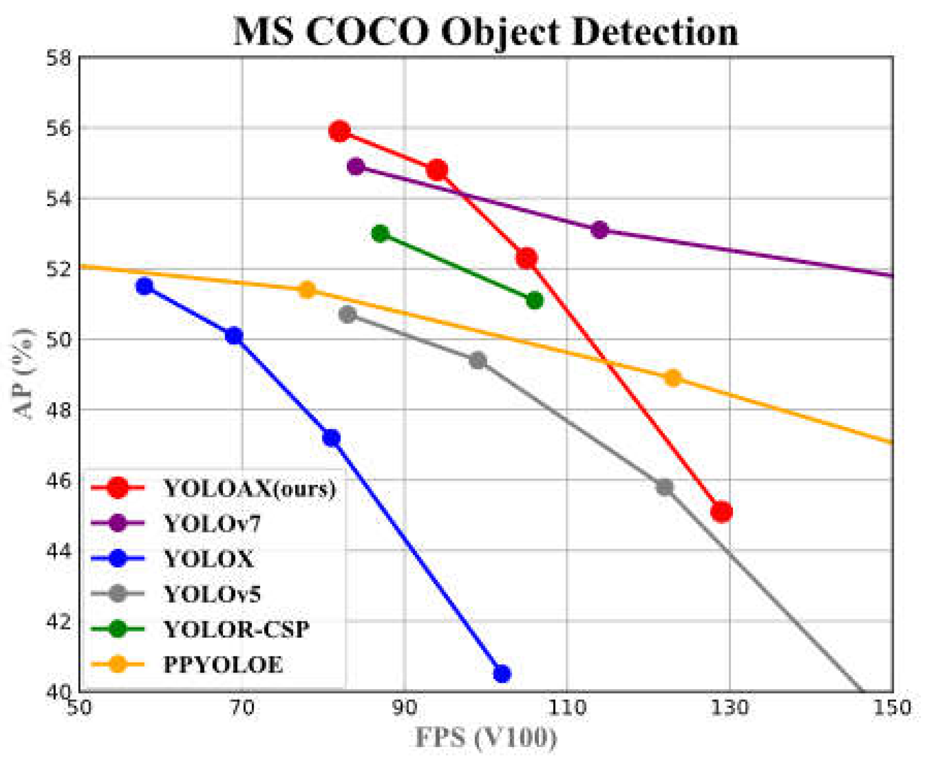
Figure 2.
The overview of our proposed architecture.
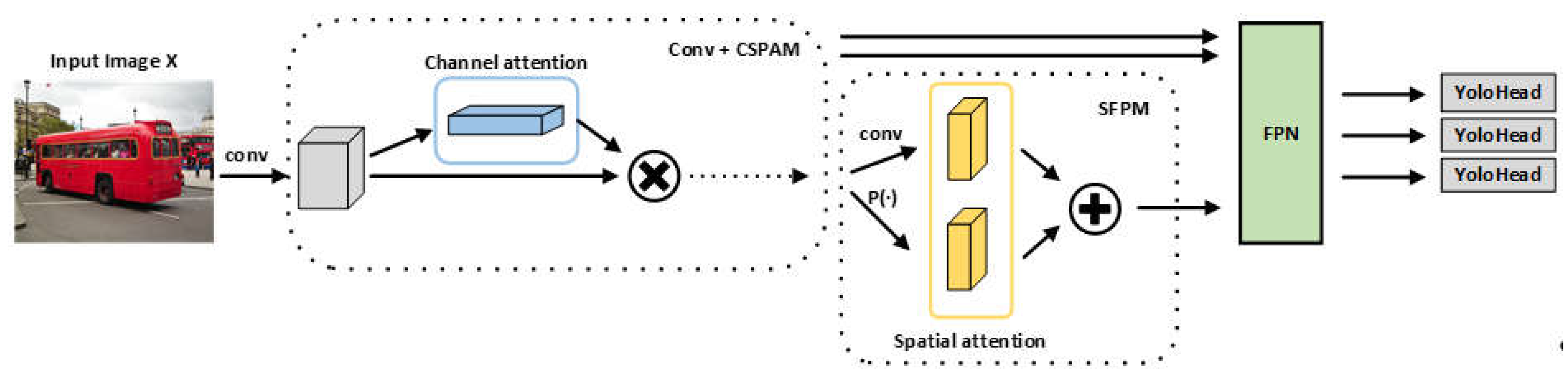
Figure 3.
(a) A single CSP layer; (b) Our proposed CSPAM. None: no information processing.
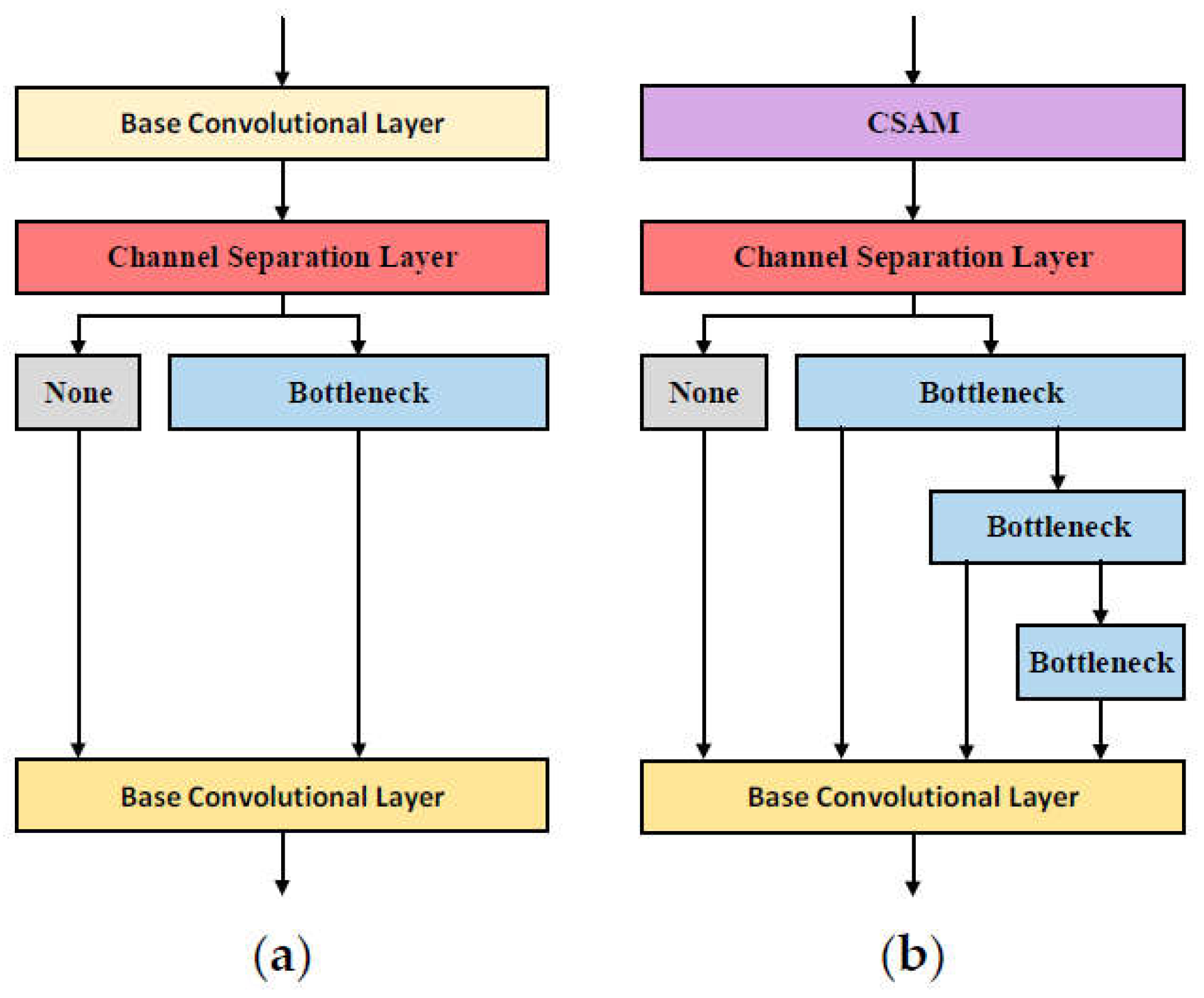
Figure 4.
The architecture of the CSAM. P(·) denote global average pooling operation and φ(·) denote 1×1 base convolutional operation.
Figure 4.
The architecture of the CSAM. P(·) denote global average pooling operation and φ(·) denote 1×1 base convolutional operation.
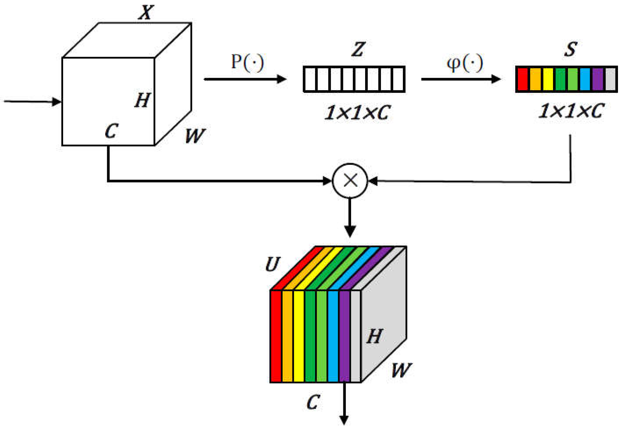
Figure 5.
Overview of our proposed SFPM. g and c denote global pooling feature and convolutional feature extractors. A: feature aggregation.
Figure 5.
Overview of our proposed SFPM. g and c denote global pooling feature and convolutional feature extractors. A: feature aggregation.
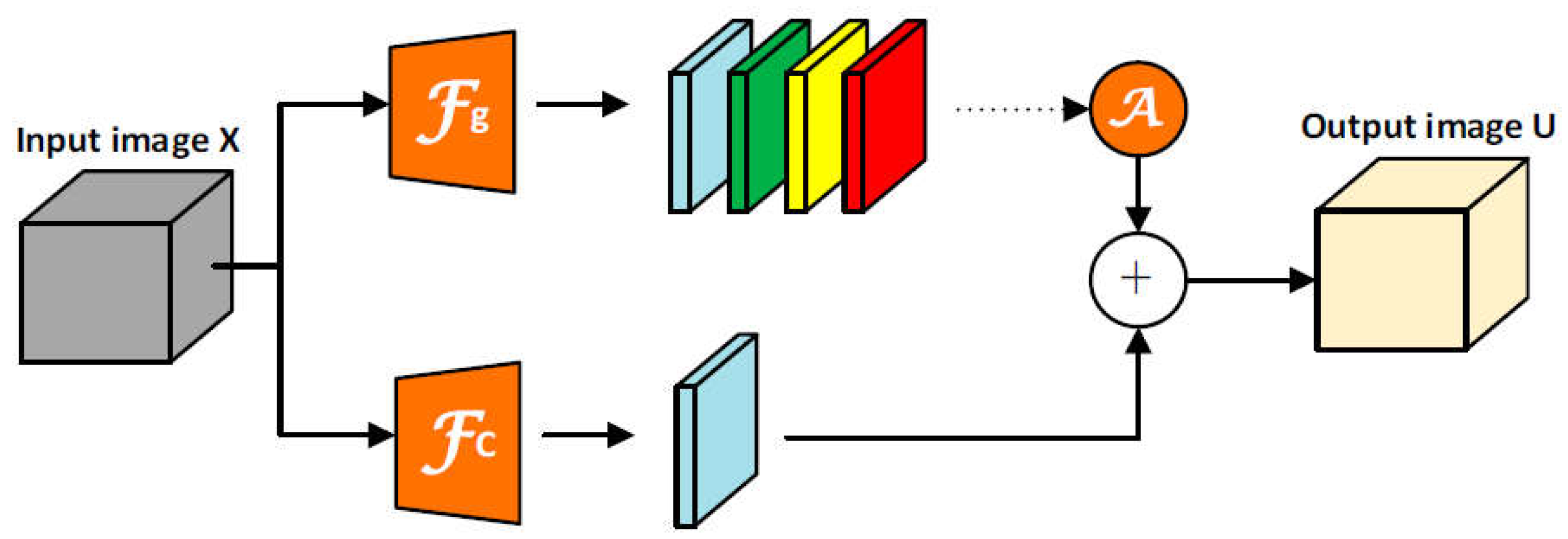
Figure 6.
Demonstration of the main difference between the head of YOLOX and our proposed decoupled head.
Figure 6.
Demonstration of the main difference between the head of YOLOX and our proposed decoupled head.
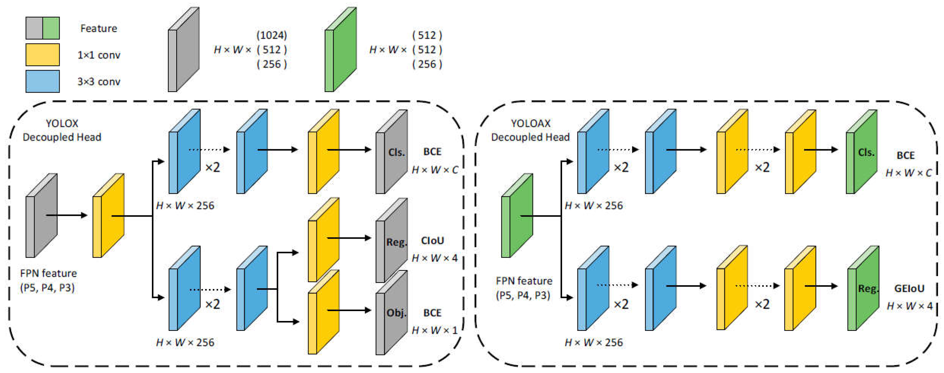
Figure 7.
The visualization results of heatmap. We take a comparison on the visualization results of heatmap of CSPAM-integrated detector (YOLOX + CSPAM) with baseline (YOLOX).
Figure 7.
The visualization results of heatmap. We take a comparison on the visualization results of heatmap of CSPAM-integrated detector (YOLOX + CSPAM) with baseline (YOLOX).
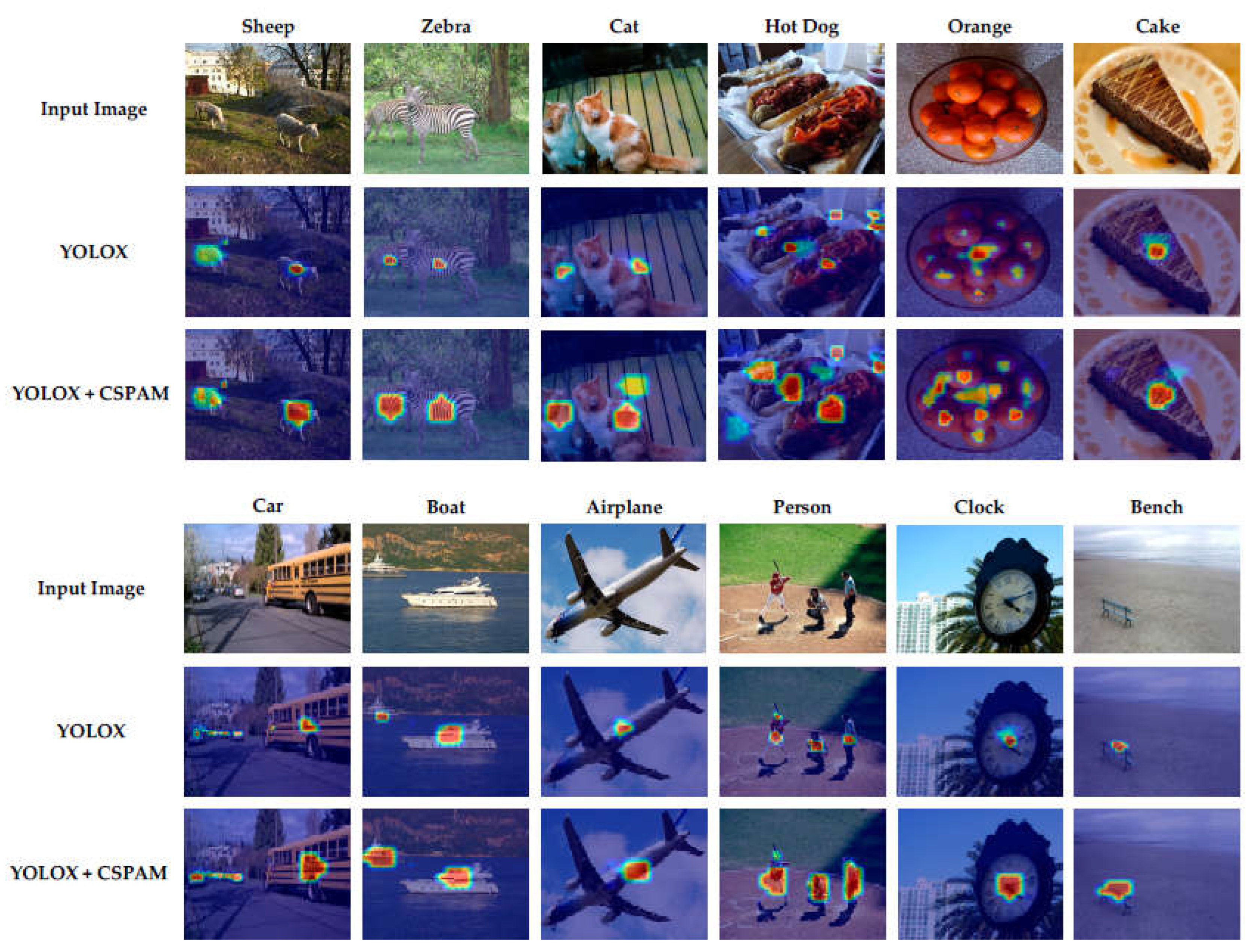
Figure 8.
Comparison of performance gains (left) and object classification loss (right).
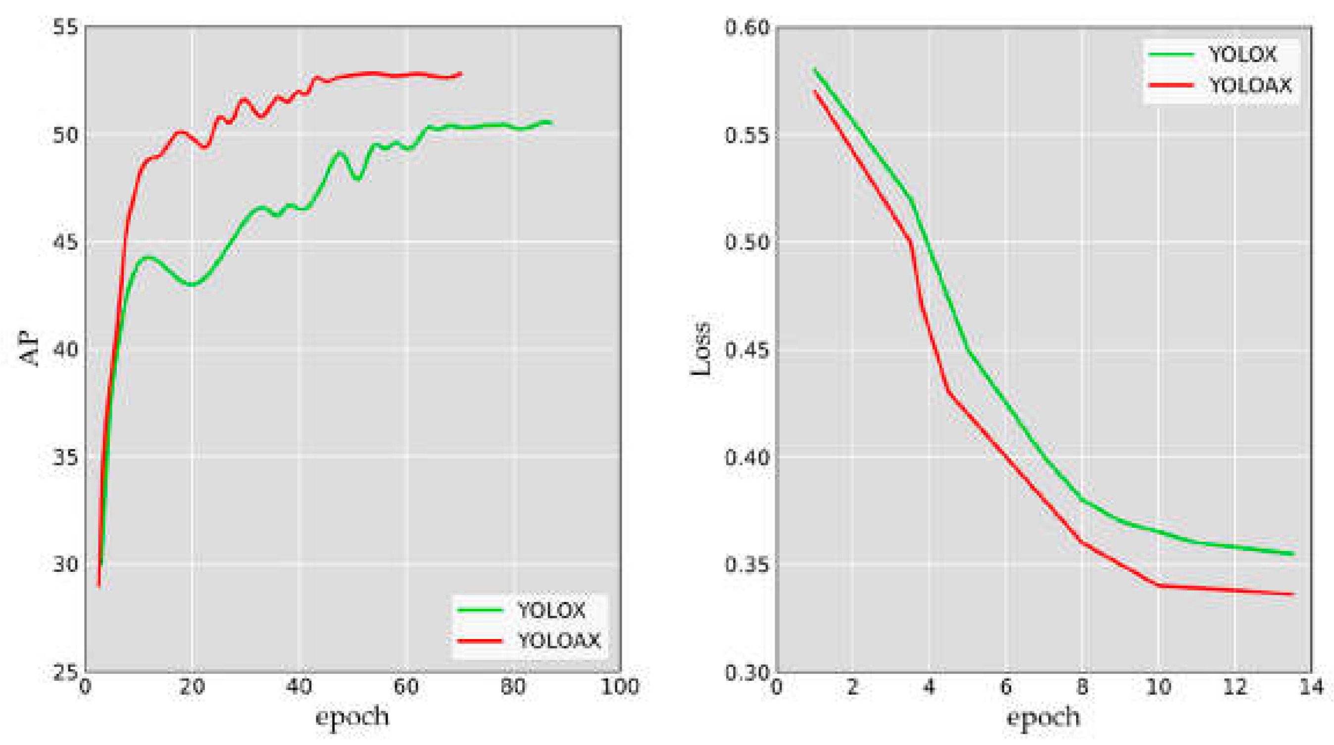
Figure 9.
Our YOLOAX and other real-time object detector visualization results.
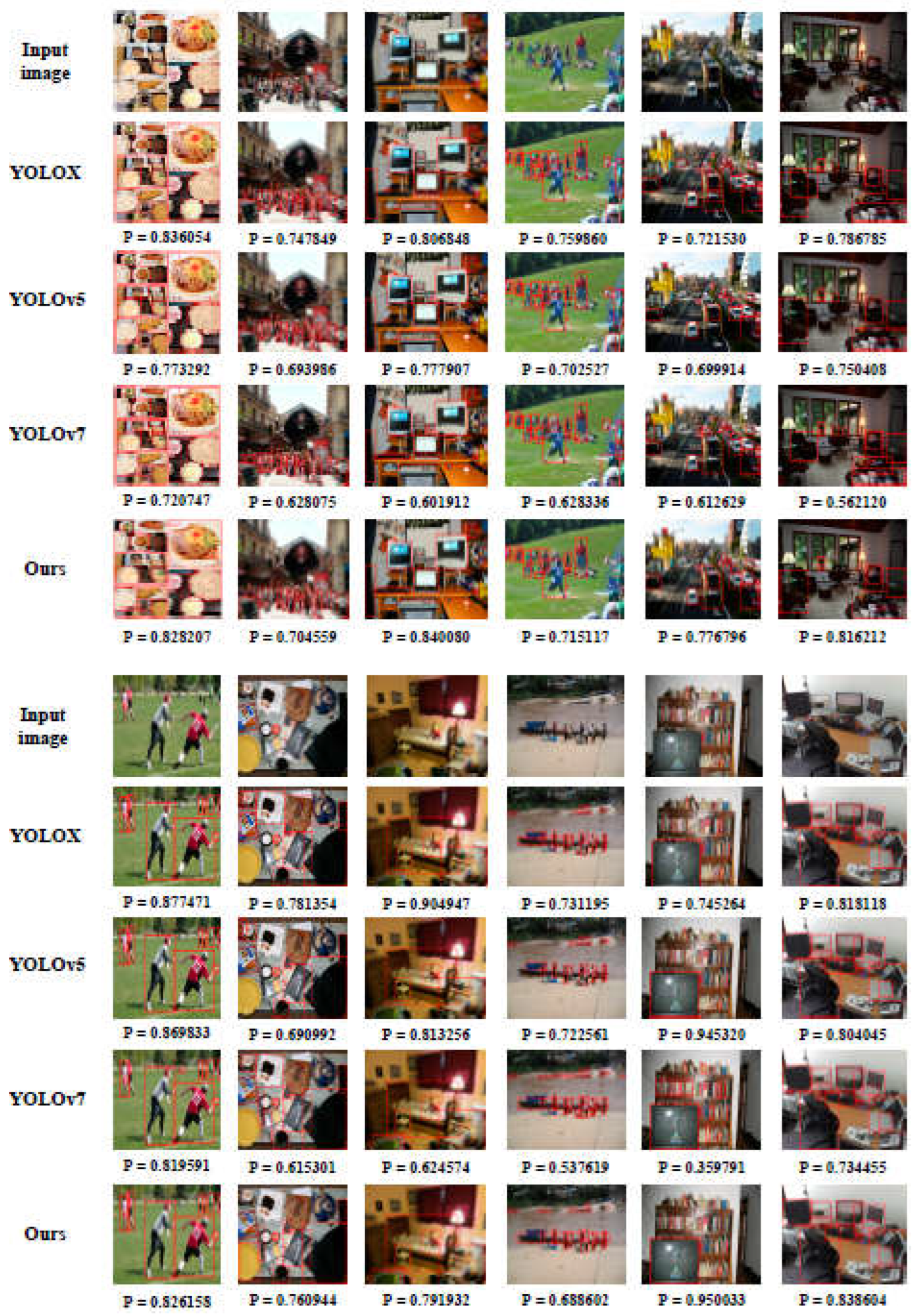

Table 1.
Effect of data augmentation across different size of models.
| Model | Mosaic | Mix-up | AP (%) |
|---|---|---|---|
| YOLOAX-S | √ | 45.1 | |
| √ | √ | 44.8 (-0.3) | |
| YOLOAX-X | √ | 53.9 | |
| √ | √ | 55.2 (+1.3) |
Table 2.
Ablation study on our CSPAM on COCO.
| Model | CSPAM | AP (%) | Parameters | GFLOPs |
|---|---|---|---|---|
| YOLOX-S | 40.5 | 9.0 M | 26.8 | |
| √ | 40.8 | 7.8 M | 24.2 | |
| improvement | + 0.3 | - 1.2 | - 2.6 | |
| YOLOX-M | 47.2 | 25.3 M | 73.8 | |
| √ | 47.4 | 22.2 M | 73.2 | |
| improvement | + 0.2 | - 3.1 | - 0.6 |
Table 3.
Ablation study on our CSPAM on PASCAL VOC.
| Model | CSPAM | AP (%) | Parameters | GFLOPs |
|---|---|---|---|---|
| YOLOX-S | 81.5 | 9.0 M | 26.8 | |
| √ | 82.6 | 7.8 M | 24.1 | |
| improvement | + 1.1 | - 1.2 | - 2.7 | |
| YOLOX-M | 83.2 | 25.3 M | 73.8 | |
| √ | 83.7 | 22.2 M | 73.2 | |
| improvement | + 0.5 | - 3.1 | - 0.6 |
Table 4.
Ablation studies on our proposed STA on MS COCO.
| Method | |||
|---|---|---|---|
| base (FCOS) | 41.5 | 60.7 | 45.0 |
| + STA (ours) | 43.2 (+1.7) | 63.8 (+3.1) | 47.2 (+2.2) |
| base (RetinaNet) | 39.1 | 59.1 | 42.3 |
| + STA (ours) | 41.8 (+2.7) | 60.4 (+1.3) | 43.5 (+1.5) |
| base (YOLOX) | 47.2 | 65.4 | 50.6 |
| + STA (ours) | 47.5 (+0.3) | 65.8 (+0.4) | 50.8 (+0.2) |
| base (YOLOAX) | 51.0 | 69.4 | 53.6 |
| + SimOTA | 51.5 (+0.5) | 69.8 (+0.4) | 53.9 (+0.3) |
| + STA (ours) | 52.3 (+1.3) | 70.5 (+1.1) | 54.3 (+0.7) |
Table 5.
Comparison of GEIOU Loss and the other counterparts IOU Loss in terms of AP (%) on COCO / PASCAL VOC.
Table 5.
Comparison of GEIOU Loss and the other counterparts IOU Loss in terms of AP (%) on COCO / PASCAL VOC.
| Method | |||
|---|---|---|---|
| Baseline | 47.2 / 64.4 | 65.4 / 85.9 | 50.6 / 72.0 |
| GIOU | 43.1 / 64.9 | 62.3 / 86.0 | 46.8 / 72.3 |
| DIOU | 43.2 / 66.1 | 63.6 / 86.4 | 47.0 / 73.1 |
| CIOU | 45.1 / 66.5 | 64.9 / 86.8 | 48.1 / 73.5 |
| EIOU | 46.3 / 66.8 | 65.4 / 87.0 | 48.8 / 73.7 |
| GEIOU (ours) | 47.4 / 67.2 | 65.5 / 87.3 | 50.7 / 74.0 |
Table 6.
Comparison of YOLOAX series and YOLOX series in terms of AP (%) on COCO, higher is better.
| Method | AP (%) | #Param. | GFLOPs | Latency |
|---|---|---|---|---|
| YOLOX-S | 39.6 | 9.0M | 26.8 | 9.8ms |
| YOLOAX-S | 45.1 (+5.5) | 7.9M | 36.3 | 10.9ms |
| YOLOX-M | 46.4 | 25.3M | 73.8 | 12.3ms |
| YOLOAX-M | 52.3 (+5.9) | 22.2M | 82.4 | 13.5ms |
| YOLOX-L | 50.0 | 54.2M | 155.6 | 14.5ms |
| YOLOAX-L | 54.8 (+4.8) | 47.6M | 172.7 | 15.3ms |
| YOLOX-X | 51.2 | 99.1M | 281.9 | 17.3ms |
| YOLOAX-X | 55.2 (+4.0) | 87.0M | 296.6 | 18.7ms |
Table 7.
Comparison of other state-of-the-arts in real-time object detection.
| Model | Backbone | #Param. | FLOPs | Size | FPS | |||
|---|---|---|---|---|---|---|---|---|
| PPYOLOE-S [6] | CSPResNet | 7.9M | 17.4G | 640 | 208 | 43.1 / 42.7 | 60.5 | 46.6 |
| PPYOLOE-M [6] | CSPResNet | 23.4M | 49.9G | 640 | 123 | 48.9 / 48.6 | 66.5 | 53.0 |
| PPYOLOE-L [6] | CSPResNet | 52.2M | 110.1G | 640 | 78 | 51.4 / 50.9 | 68.9 | 55.6 |
| PPYOLOE-X [6] | CSPResNet | 98.4M | 206.6G | 640 | 45 | 52.2 / 51.9 | 69.9 | 56.5 |
| YOLOv7 [10] | - | 36.9M | 104.7G | 640 | 161 | 51.4 / 51.2 | 69.7 | 55.9 |
| YOLOv7-X [10] | - | 71.3M | 189.9G | 640 | 114 | 53.1 / 52.9 | 71.2 | 57.8 |
| YOLOv7-W6 [10] | - | 70.4M | 360.0G | 1280 | 84 | 54.9 / 54.6 | 72.6 | 60.1 |
| YOLOR-CSP [8] | Modified CSP v5 | 52.9M | 120.4G | 640 | 106 | 51.1 / 50.8 | 69.6 | 55.7 |
| YOLOR-CSP-X [8] | Modified CSP v5 | 96.9M | 226.8G | 640 | 87 | 53.0 / 52.7 | 71.4 | 57.9 |
| YOLOX-S [9] | Darknet-53 | 9.0M | 26.8G | 640 | 102 | 40.5 / 40.5 | - | - |
| YOLOX-M [9] | Modified CSP v5 | 25.3M | 73.8G | 640 | 81 | 47.2 / 46.9 | 65.4 | 50.6 |
| YOLOX-L [9] | Modified CSP v5 | 54.2M | 155.6G | 640 | 69 | 50.1 / 49.7 | 68.5 | 54.5 |
| YOLOX-X [9] | Modified CSP v5 | 99.1M | 281.9G | 640 | 58 | 51.5 / 51.1 | 69.6 | 55.7 |
| F-RCNN-FPN+ [1] | ResNet 101 | 60.0M | 246.0G | 1333 | 20 | - / 44.0 | - | - |
| DETR DC5 [35] | ResNet 101 | 60.0M | 253.0G | 1333 | 10 | - / 44.9 | - | - |
| Swin-L [16] | - | - | 1382.0G | 1280 | 9.2 | - / 53.9 | 72.4 | 58.8 |
| YOLOAX-S | CSPDarknet | 7.9M | 36.3G | 640 | 129 | 45.1 / 45.0 | 62.8 | 47.7 |
| YOLOAX-M | CSPDarknet | 22.2M | 82.4G | 640 | 105 | 52.3 / 52.0 | 70.5 | 54.3 |
| YOLOAX-L | CSPDarknet | 47.6M | 172.7G | 640 | 94 | 54.8 / 54.5 | 72.2 | 58.2 |
| YOLOAX-X | CSPDarknet | 87.0M | 296.6G | 640 | 82 | 55.2 / 55.0 | 73.1 | 60.6 |
Disclaimer/Publisher’s Note: The statements, opinions and data contained in all publications are solely those of the individual author(s) and contributor(s) and not of MDPI and/or the editor(s). MDPI and/or the editor(s) disclaim responsibility for any injury to people or property resulting from any ideas, methods, instructions or products referred to in the content. |
© 2024 by the authors. Licensee MDPI, Basel, Switzerland. This article is an open access article distributed under the terms and conditions of the Creative Commons Attribution (CC BY) license (http://creativecommons.org/licenses/by/4.0/).
Copyright: This open access article is published under a Creative Commons CC BY 4.0 license, which permit the free download, distribution, and reuse, provided that the author and preprint are cited in any reuse.


