

Submitted:
06 May 2024
Posted:
07 May 2024
You are already at the latest version
Abstract
This paper presents a statistical approach to identify the underlying roughness characteristics in synthetic aperture radar (SAR) intensity data. The physical modeling of this kind of data allows the use of the Gamma distribution in the presence of fully-developed speckle, i.e., when there are infinitely many independent backscatterers per resolution cell, and none dominates the return. Such areas are often called ``homogeneous'' or ``textureless'' regions. The GI0 distribution is also a widely accepted law for heterogeneous and extremely heterogeneous regions, i.e., areas where the fully-developed speckle hypotheses do not hold. We propose three test statistics to distinguish between homogeneous and inhomogeneous regions, i.e., between gamma and GI0 distributed data, both with a known number of looks. The first test statistic uses a bootstrapped non-parametric estimator of Shannon entropy, providing a robust assessment in uncertain distributional assumptions. The second test uses the classical coefficient of variation (CV). The third test uses an alternative form of estimating the CV based on the ratio of the mean absolute deviation from the median to the median. We apply our test statistic to create maps of \(p\)-values for the homogeneity hypothesis. Finally, we show that our proposal, the entropy-based test, outperforms existing methods, such as the classical CV and its alternative variant, in identifying heterogeneity when applied to both simulated and actual data.
Keywords:
SAR
; heterogeneity
; entropy
; coefficient of variation
; hypothesis tests
1. Introduction
Synthetic Aperture Radar (SAR) technology has become essential for environmental monitoring and disaster management. It provides valuable images under various conditions, including day or night and weather situations [1,2]. However, the effective use of SAR data depends on a thorough understanding of its statistical properties because it is corrupted by speckle. This noise-like interference effect is inherent in SAR data due to the coherent nature of the imaging process [3].
Speckle in intensity format is non-Gaussian. Thus, SAR data require reliable statistical models for accurate processing. The distribution, which is suitable for SAR data, includes the Gamma law as the limiting case for fully-developed speckle [4] and provides flexibility with fewer parameters for analysis.
Our work aims to improve the identification of potential roughness features in SAR intensity data. Physical modeling of SAR data allows the use of the Gamma distribution in the presence of fully-developed speckle, where an infinite number of independent backscatterers per resolution unit is assumed, commonly referred to as homogeneous regions.
In this context, we present a set of three novel test statistics that aim to distinguish between homogeneous and non-homogeneous returns, particularly between gamma and distributed data, assuming the number of looks is known. We use properties such as entropy and coefficient of variation.
Entropy is a fundamental concept in information theory with far-reaching applications in pattern recognition, statistical physics, image processing, edge detection and SAR image analysis [5,6,7,8,9]. Shannon introduced it in 1948 [10] for a random variable to measure information and uncertainty. Shannon entropy is a crucial descriptive parameter in statistics, especially for evaluating data dispersion and performing tests for normality, exponentiality and uniformity [11,12]. Entropy estimation is challenging, especially when the model is unknown. In these cases, non-parametric methods are used. Spacing methods have been discussed as a non-parametric approach in Refs. [13,14]. This strategy is flexible and robust because it does not enforce a model or parametric constraints.
The coefficient of variation (CV), introduced in 1896 by Pearson [15], is a relative dispersion measure widely used in various fields of applied statistics, including sampling, biostatistics, medical and biological research, climatology and other fields [16,17,18,19]. It facilitates the comparison of variability between different populations and is particularly valuable for relating variables with different units. This is because when the primary purpose is to compare the variations of several variables, the standard deviation can only serve as an adequate measure of variation if all variables are expressed in the same unit of measurement and have identical means. If these conditions are not met, then the CV is the relative measure that is usually used in real applications. The variable with the highest CV value has the largest relative dispersion around the mean value [20]. The coefficient of variation is the primary measure of heterogeneity in SAR data [21,22]. We study two ways of estimating the coefficient of variation.
The other parameter we study is the Shannon entropy. Different roughness levels materialized as models for SAR data, have different entropy values, but this fundamental quantity can also be estimated in a model-agnostic way. We exploit this property and design a bootstrap-improved non-parametric estimator for the Shannon entropy.
We devise test statistics based on these three estimators: the classical coefficient of variation, a robust version, and the Shannon entropy estimator. We apply these test statistics to generate maps of evidence of homogeneity that reveal different types of targets in the SAR data. We show that our proposed method is superior to existing approaches with simulated data and SAR images.
The article is structured as follows: Section 2 deals with statistical modeling and entropy estimation for intensity SAR data. Section 3 outlines hypothesis tests based on non-parametric entropy and coefficients of variation estimators. In Section 4 we present experimental results. Finally, we draw conclusions in Section 5.
2. Background
2.1. Statistical Modeling of Intensity SAR Data
The primary models for intensity SAR data include the Gamma and distributions [23]. The first is suitable for fully-developed speckle and is a limiting case of the second model. This is interesting due to its versatility in accurately representing regions with different roughness properties [24]. We denote and to indicate that Z follows the distributions characterized by the respective probability density functions (pdfs):
and
where is the mean, is the scale, measures the roughness, is the number of looks, is the gamma function, and is the indicator function of the set A.
The rth order moments of the model are
provided , and infinite otherwise. Therefore, assuming , its expected value is
2.2. The Shannon Entropy
The parametric representation of Shannon entropy for a system described by a continuous random variable is:
here, is the pdf that characterizes the distribution of the real-valued random variable Z.
Using (6), we obtain the Shannon entropy of in (1) and in (5):
where is the digamma function. Figure 1, shows the entropy of as a function of when . Notice that it converges to the entropy of when , as expected. The more heterogeneous (large values) the SAR region is, the larger the entropy (or degree of disorder) is.
2.3. Estimation of the Shannon Entropy
The problem of the non-parametric estimation of has been studied by many authors, including [11,26,27,28]. Their proposals use estimators based on differences between order statistics: spacings.
Vasicek [26] introduced one of the first non-parametric estimators based on spacings. Under the assumption that is a random sample from the distribution , the estimator is defined as:
where is a positive integer, are the order statistics, and is the m-spacing, in which if , if .
Several authors have explored adaptations to Vasicek’s estimator. We consider three estimators known for their superior performance [24]:
- Correa [27]:where , , for and for . Based on simulations, he showed that his estimator has a smaller mean square error than Vasicek’s approach.
These estimators are asymptotically consistent, i.e., they converge in probability to the true value when and . However, we will use improved bootstrap-improved versions because we need them to perform well with small samples.
2.4. Enhanced Estimators with Bootstrap
We use the bootstrap technique to refine the accuracy of non-parametric entropy estimators. In this approach, new data sets are generated by replicate sampling from an existing data set [31].
Let us assume that the non-parametric entropy estimator is inherently biased, i.e,:
Our bootstrap-improved estimator is of the form:
where B is the number of observations obtained by resampling from with replacement. Applying this methodology, the original estimators of Correa, Ebrahimi and Al-Omari are now referred to as the proposed bootstrap-improved versions: , , and , respectively.
We analyzed the performance of these estimators with a Monte Carlo study: 1000 samples from the distribution of size , with and . The results are consistent with other situations. We used bootstrap samples and the heuristic spacing , as recommended in the literature.
In Figure 2 we show the bias and mean squared error (MSE) of the original non-parametric entropy estimators and their respective bootstrap-enhanced versions. Bootstrap-enhanced estimators have smaller bias and MSE, especially for sample sizes below 81. The results of the simulation can be found in Table 1.
2.5. Coefficient of Variation and a Robust Alternative
The population CV is defined as a ratio of the population standard deviation to the population mean :
The CV can be easily estimated as the ratio of the sample mean to the sample standard deviation.
We explore a robust alternative to estimate the CV, as described by [32]: the ratio between the mean absolute deviation from the median (MnAD) and the median, two well-known robust measures of scale and location, respectively. The sample version for the MnAD is defined as , where is an estimate for the median of the population, for example, the sample median.
3. Hypothesis Testing
We aim to test the following hypotheses:
We are testing the hypothesis that the data are fully-developed speckle versus the alternative of data with roughness. As for the parametric problem, once it is not possible to define the hypothesis , it is impossible to solve this problem with parametric inference alternatives (such as likelihood ratio, score, gradient, and Wald hypothesis test). The proposed tests to solve this physical problem in SAR systems are described below.
3.1. The Proposed Test Based on Non-Parametric Entropy
For a random sample from a distribution , a test statistic is proposed. It is based on an empirical distribution that arises from the difference between non-parametrically estimated entropies and the analytical entropy of (7) evaluated at the logarithm of the sample mean, where is known.
Hence, the entropy-based test statistic is defined as:
This test statistic aims to assess the behavior of the data under the null hypothesis using the empirical distribution. If the data represent fully-developed speckle, the density should center around zero, i.e., . Otherwise, the empirical distribution would shift from zero under the alternative hypothesis, suggesting significant differences and heterogeneous clutter.
The comparison between the bootstrap-improved estimators is shown in Table 2, where the test accuracy under the null hypothesis is presented alongside running times. The test accuracy is evaluated through 1000 simulated samples of different sizes, with each size replicated 100 times using bootstrap resampling.
The processing time is an important feature, especially considering the application of these estimators to large datasets of SAR images, as seen in Section 4.
As visible from Table 2, the accuracy of the test results across the three estimators shows similarities in specific sample sizes. However, practical scenarios in SAR image processing often involve small sample sizes, typically obtained over windows of size .
It is also noteworthy that the estimator exhibited the shortest processing time, followed by and . Considering this aspect, we select the estimator for subsequent simulations. Henceforth, the test statistical (13) will be denoted as: .
We now verify the normality of the data generated by the test. Figure 3 shows the empirical densities obtained by applying the test to different sample sizes drawn from the distribution, where L takes values and . Additionally, Table 3 summarizes the main descriptive statistics, including mean, standard deviation (SD), variance (Var), skewness (SK), excessive kurtosis (EK) and Anderson–Darling p values for normality. Results with p values greater than do not indicate a violation of the normality assumption. A low variance, skewness, and excessive kurtosis of almost zero indicate limited dispersion, asymmetry, and a light tail. Normal Q–Q plots confirm no evidence against a normal distribution, as shown in Figure 4.
After checking the data’s normality, we examined the proposed test’s abilities in terms of size and power. Under , the distribution of the test statistic is asymptotically normal. Therefore, the p values are calculated as , where is the standard Gaussian cumulative distribution function, and is the standardized test statistic given by:
We have nominal levels of 1 , 5 , and 10 . In terms of size, 1000 simulations were used for different sample sizes from the distribution, with varying values of L, and . In all cases, the nominal level was achieved. We assessed the test power using 1000 simulations for different sample sizes from the distribution, with , and . The power generally improves with increasing sample size and number of looks. The results are shown in Table 4.
3.2. The Proposed Test Based on Coefficient of Variation and a Robust Alternative
In addition to the test, we also propose a test statistic based on the classical CV. This test statistic is defined as follows:
where S and are the sample standard deviation and mean, respectively.
Similarly, we use another test statistic based on the ratio of the MnAD to the median. This statistic is given by:
We proceed to identify suitable models for these estimators of the CV, and then form test statistics.
The situations in which the use of CV and may be appropriate, i.e., when the observations are positive, the log-normal (LN) and the inverse Gaussian distribution (IG) are often more appropriate than the Gamma and Weibull distributions [33,34].
It is shown that the IG distribution is well approximated by the log-normal distribution, which means that the IG distribution also does not share the problem of the non-existence of a fixed-width confidence interval with the Gaussian case [35].
The biparametric LN distribution has density:
with is any real number, and is positive.
3.3. Model Selection Criterion
We used the Akaike information criterion (AIC) and the Bayesian information criterion (BIC) to select the best-fitting distribution.
The AIC deals with the trade-off between the goodness-of-fit and the model’s simplicity in terms of the number of model parameters [36]. The model or distribution with the lowest value of AIC is chosen to be the best. The BIC assesses goodness-of-fit of a distribution or model, but avoids overfitting by penalising additional degrees of freedom [37]. The model with the lowest BIC value is chosen as the best.
The AIC and BIC results in Table 5, Table 6, Table 7 and Table 8 indicate that the CV and data from different distributed and synthetic sample sizes match the properties of an LN distribution. It is important to note that this conclusion was drawn empirically based on a dictionary of analytically tractable distributions and well-defined under biparametric, unimodal, asymmetric, and positive distributions.
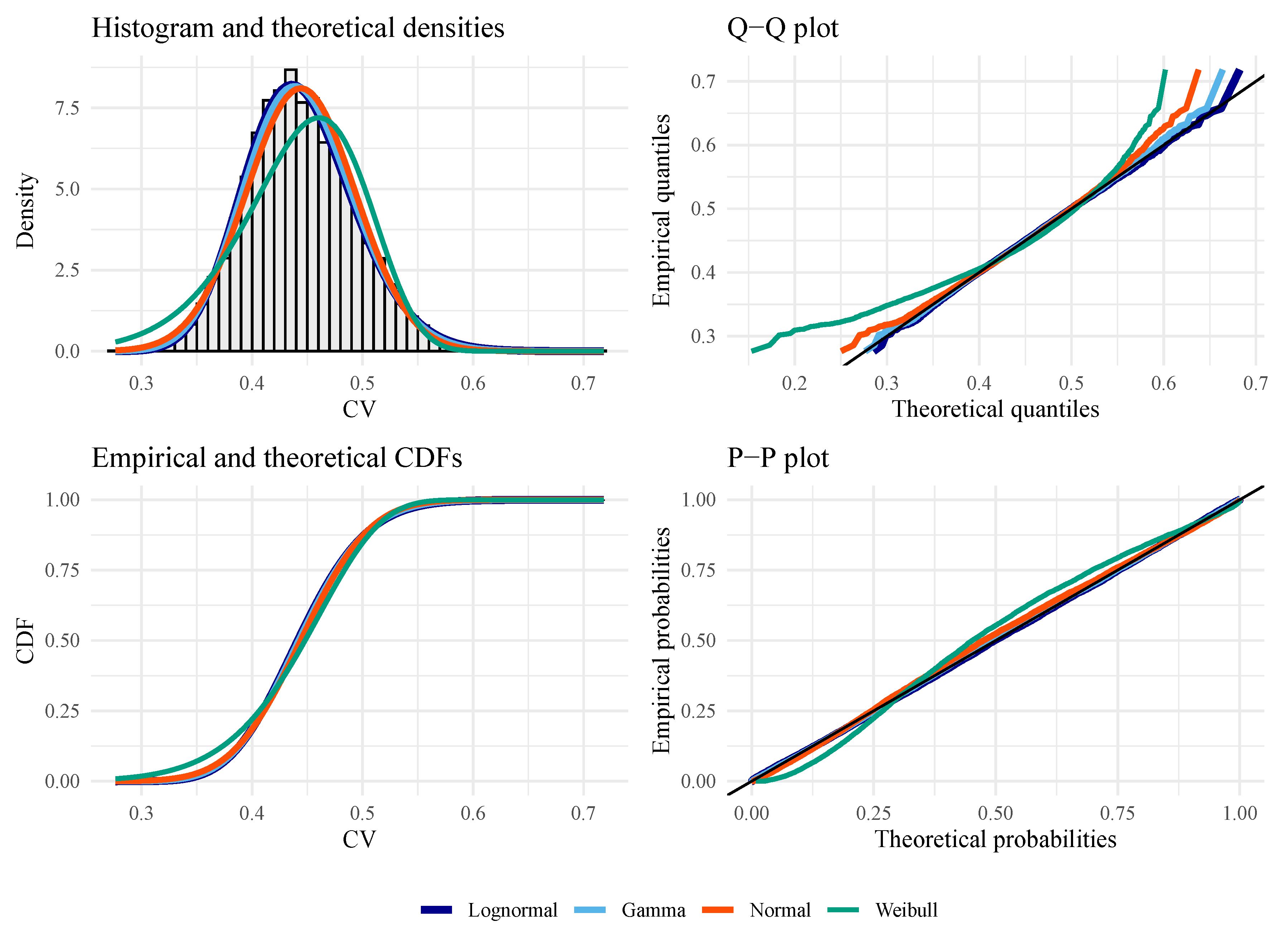
Figure 6, Figure 7 and Figure 8 show empirical and fitted density plots, Q–Q plots, P–P plots, as well as empirical and fitted cumulative distribution functions. They provide qualitative sources that confirm that the LN distribution is the most appropriate distribution. As expected, both test statistics work well under the null hypothesis. Under the alternative hypothesis, the P–P plot shows that is more robust than CV, although both statistics suffer from the tail effect caused by the distributed data.
Figure 5.
Goodness of fit plots for evaluating the best distribution with CV data from (under the null hypothesis), with , , and .
Figure 5.
Goodness of fit plots for evaluating the best distribution with CV data from (under the null hypothesis), with , , and .
4. Results
This section presents the simulations we performed to evaluate the proposed test statistics’ performance, followed by applications to SAR data.
4.1. Simulated Data
Figure 9(a) shows the phantom with dimensions of pixels. It was proposed by Gomez et al. [38] as a tool to assess the performance of speckle-reduction filters.
Figure 9(b) shows the simulated image, where each small phantom displaying texture variations. The observations are independent draws from the distribution (5), with and varying and , annotated in the image for each quadrant. Light regions correspond to textured observations (heterogeneous), while darker regions represent textureless areas (homogeneous).
The parameter of the distribution is essential for interpreting texture characteristics. Values near zero greater than suggest extremely textured targets, such as urban zones [39]. As the value decreases, it indicates regions with moderate texture (in the region), related to forest zones, while values below correspond to textureless regions, such as pasture, agricultural fields, and water bodies [40].
We applied the three test statistics, namely , , and , to the simulated image using local sliding windows of size , as shown in Figure 10(a)–(c).
The resulting p-values for each test are shown in Figure 11(a)–(c). In Figure 12(a)–(c), maps are depicted using a color table between black, gray levels, and white. All p-values above are represented in white (indicating no evidence to reject the null hypothesis), while those below are shown in black (indicating evidence to reject the hypothesis). We notice that the performs significantly better than the other tests in identifying heterogeneous areas in the simulated image.
4.2. SAR Data
We evaluated the proposed test statistics using three SAR images: one of the coast of Jalisco, Mexico (with a spatial resolution of 20 m both along azimuth and range directions) and two of Illinois, USA (with a spatial resolution of 10 both along azimuth and range directions), acquired by the Sentinel-1B satellite operating in C-band, with VV polarization and intensity format. The first two images have a size of pixels, while the third has pixels, and they contain mountainous areas, agricultural regions, water bodies, and urban areas, as shown in Figure 13(a)–(c).
The three statistical tests are applied to the SAR images using local sliding windows, as illustrated in Figure 14, Figure 17 and Figure 20.
The p-values obtained for each test are presented in Figure 15, Figure 18 and Figure 21, respectively.
In Figure 16, Figure 19 and Figure 22, the maps of p-values composed of a linear gradient of black and white colors, represent the decisions at a 5 significance level. Dark areas represent values below , indicating evidence to reject the null hypothesis and suggesting heterogeneity in these regions. In contrast, values above 0.05 are represented as white areas, indicating no evidence to reject the fully-developed speckle hypothesis.
Figure 14.
Results of applying the test statistics, Coast of Jalisco: (a) , (b) , and (c) .
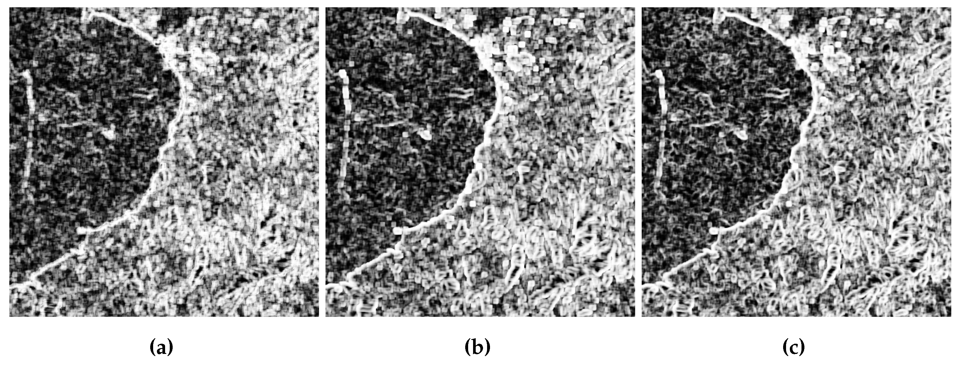
Figure 15.
Map of p-values, Coast of Jalisco: (a) . (b) . (c) .
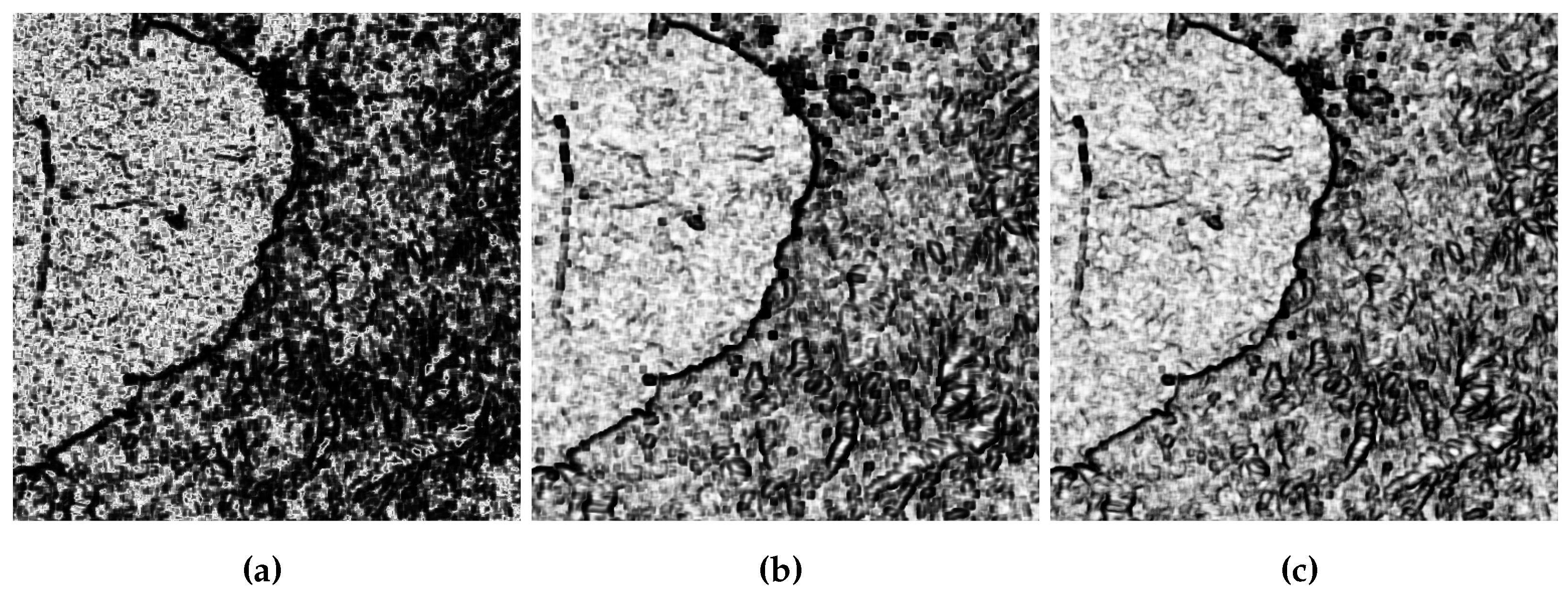
Figure 16.
Results for a threshold of of the p-value, Coast of Jalisco. (a) , (b) , and (c) .
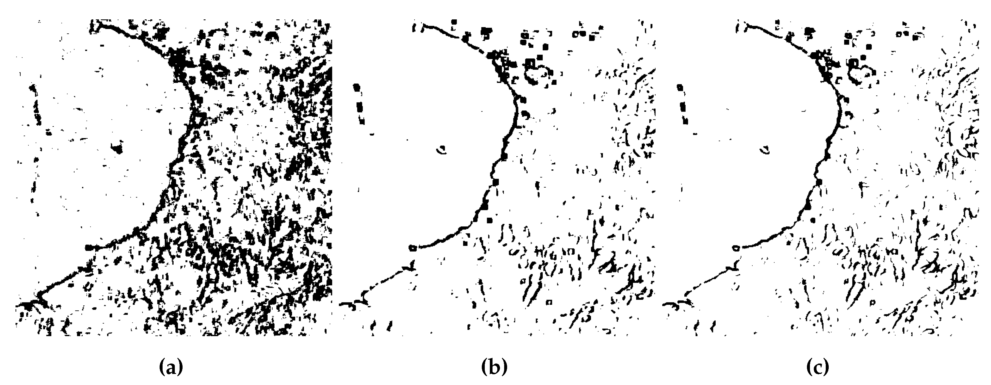
Figure 17.
Results of applying the test statistics, Illinois-Region 1: (a) , (b) , and (c) .

Figure 18.
Map of p-values, Illinois-Region 1: (a) , (b) , and (c) .
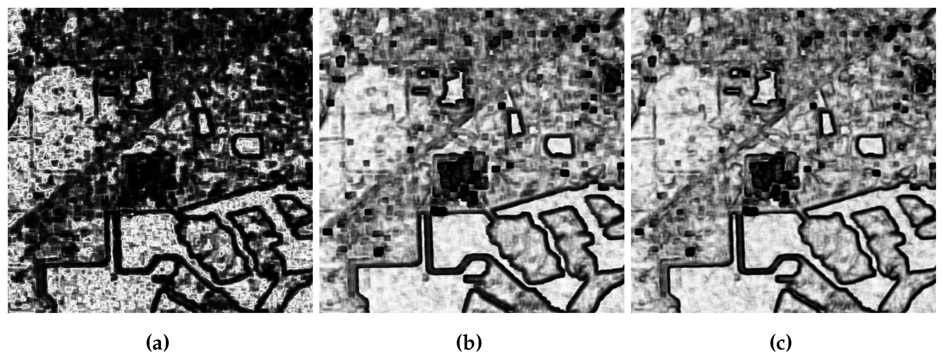
Figure 19.
Results for a threshold of of the p-value, Illinois-Region 1. (a) , (b) , and (c) .
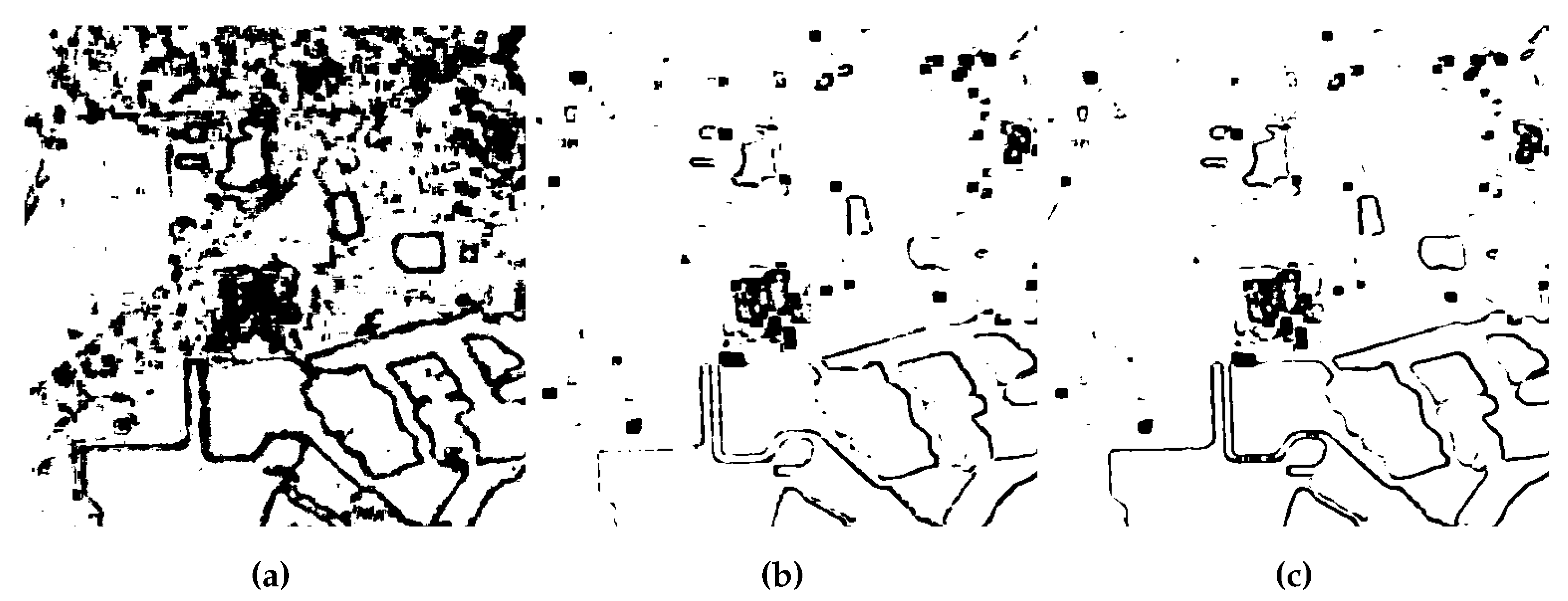
Using Shannon entropy is more meaningful than using the original and robust CV to capture heterogeneity. It is justified that the dark areas of the maps based on the and show coverage patterns similar to those reported for the map. This suggests that although CV-based tests may produce slightly less pronounced results than the entropy-based test, they still demonstrate a comparable ability to detect heterogeneity within SAR images.
Figure 20.
Results of applying the test statistics, Illinois-Region 2: (a) , (b) , and (c) .
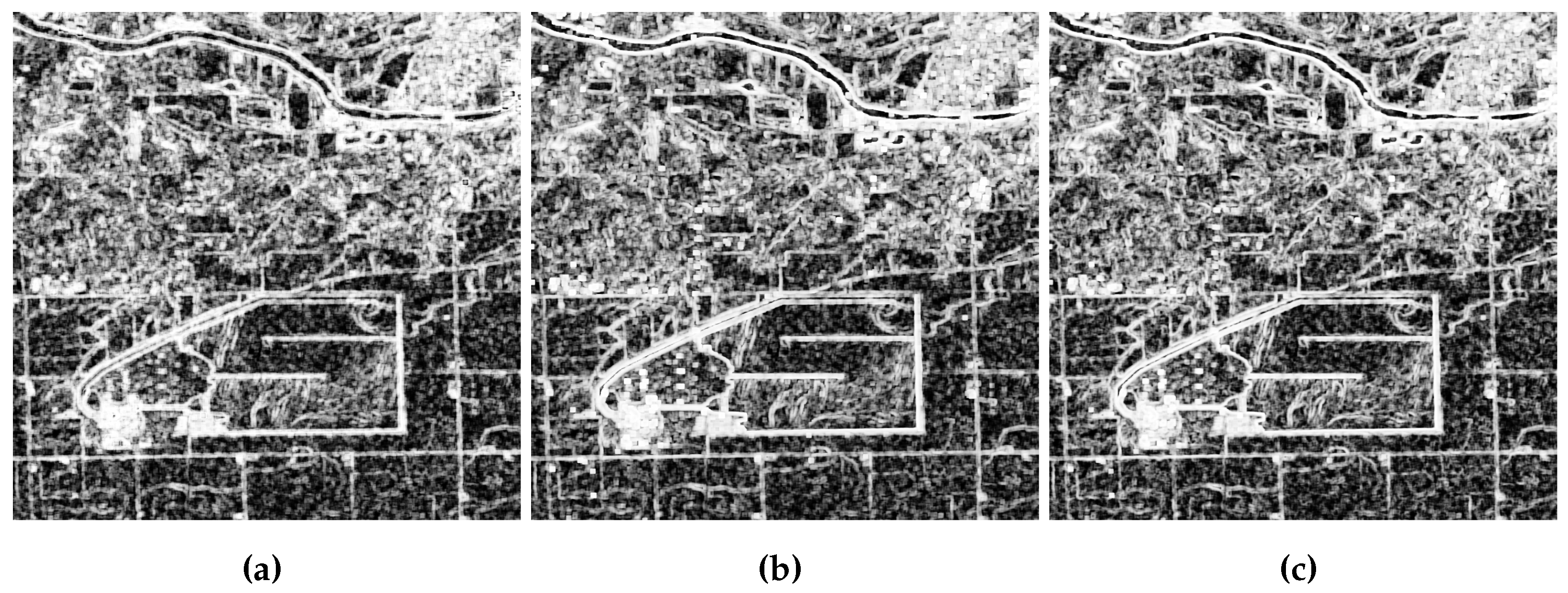
Figure 21.
Map of p-values, Illinois-Region 2: (a) , (b) , and (c) .
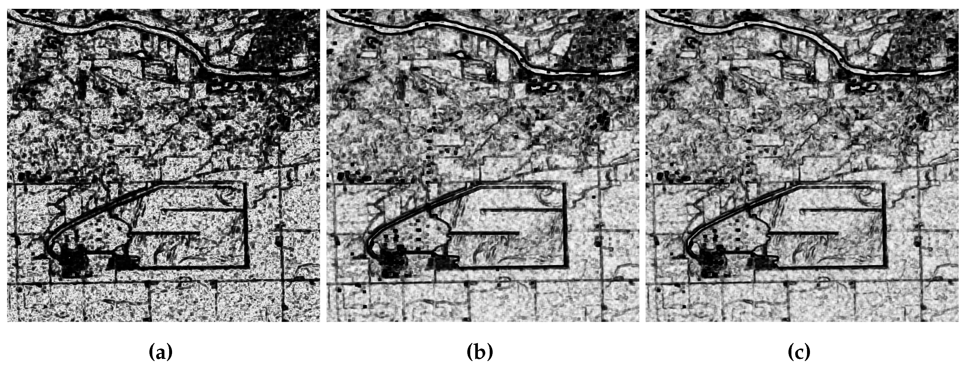
Figure 22.
Results for a threshold of of the p-value, Illinois-Region 2. (a) , (b) , and (c) .
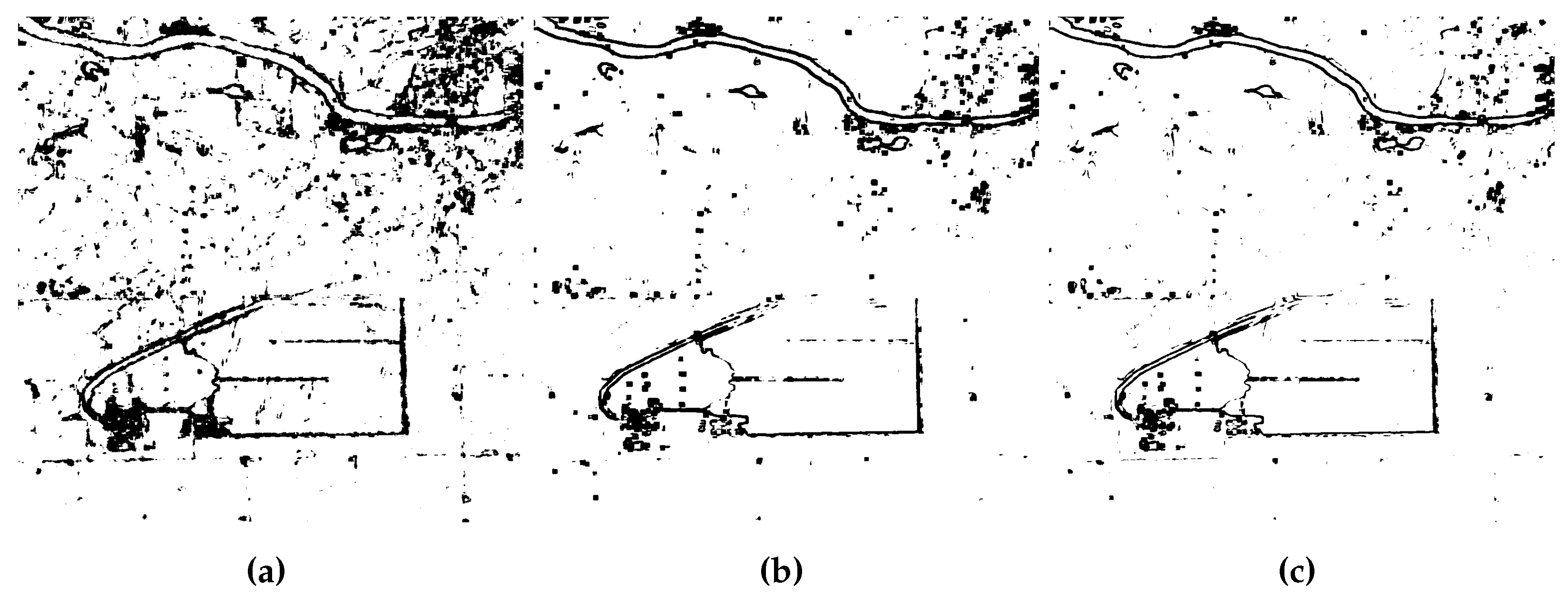
It is noticeable that the entropy and CV-based tools predicted heterogeneity regions and boundaries where the statistical properties of texture vary. The test was shown to be an effective edge detector. It emerges as a robust alternative to the classical CV test, making it less susceptible to the influence of outliers and allowing it to produce more precise edges. Considering a higher significance level may increase the sensitivity to edge detection but also increase the risk of detecting false heterogeneous regions.
5. Conclusions
This article provides a practical and theoretical answer to the following physical question: How to detect heterogeneity in SAR images, assuming that the SAR intensity follows the model. To this end, we proposed three novel hypothesis tests, one from the Shannon entropy and two from the variation coefficient variants. The performance of our proposals was evaluated using a Monte Carlo study. The results showed that they were conservative in estimating the probability of a type I error (false alarm rate) and the test power (probability of detection), which increases with sample size. An application to three recent SAR images was performed. The results showed that the Shannon entropy-based test was more robust than the CV-based tests. In addition, all tests could recognize images with different textures and identify edges where the texture type changes.
Supplementary Materials
This article was written in Rmarkdown and is fully reproducible. The code and data are accessible at https://github.com/rjaneth/identifying-heterogeneity-in-sar-data-with-new-test-statistics (accessed on 30 April 2024).
Author Contributions
All authors (A.C.F., J.A, and A.D.C.N.) discussed the results and contributed to the research. All authors have read and agreed to the published version of the manuscript.
Funding
This research received no external funding.
Institutional Review Board Statement
Not applicable.
Data Availability Statement
The Sentinel-1 images are made publicly available by the European Space Agency via Copernicus Data Space Ecosystem at https://dataspace.copernicus.eu/ (accessed on 24 April 2024).
Acknowledgments
The author J.A. would like to thank the Coordenação de Aperfeiçoamento de Pessoal de Nível Superior (CAPES) and the Fundação de Amparo à Ciência e Tecnologia de Pernambuco (FACEPE) for their support.
Conflicts of Interest
The authors declare no conflict of interest.
References
- Moreira, A.; Prats-Iraola, P.; Younis, M.; Krieger, G.; Hajnsek, I.; Papathanassiou, K.P. A tutorial on synthetic aperture radar. IEEE Geoscience and Remote Sensing Magazine 2013, 1, 6–43. [Google Scholar] [CrossRef]
- Mu, Y.; Huang, B.; Pan, Z.; Yang, H.; Hou, G.; Duan, J. An Enhanced High-Order Variational Model Based on Speckle Noise Removal With G0 Distribution. IEEE Access 2019, 7, 104365–104379. [Google Scholar] [CrossRef]
- Argenti, F.; Lapini, A.; Bianchi, T.; Alparone, L. A Tutorial on Speckle Reduction in Synthetic Aperture Radar Images. IEEE Geoscience and Remote Sensing Magazine 2013, 1, 6–35. [Google Scholar] [CrossRef]
- de, A. Ferreira, J.; Nascimento, A.D.C. Shannon Entropy for the GI0 Model: A New Segmentation Approach. IEEE J. Sel. Top. Appl. Earth Obs. Remote Sens. 2020, 13, 2547–2553. [Google Scholar]
- Pressé, S.; Ghosh, K.; Lee, J.; Dill, K.A. Principles of maximum entropy and maximum caliber in statistical physics. Reviews of Modern Physics 2013, 85, 1115–1141. [Google Scholar] [CrossRef]
- Mohammad-Djafari, A. Entropy, Information Theory, Information Geometry and Bayesian Inference in Data, Signal and Image Processing and Inverse Problems. Entropy 2015, 17, 3989–4027. [Google Scholar] [CrossRef]
- Avval, T.G.; Moeini, B.; Carver, V.; Fairley, N.; Smith, E.F.; Baltrusaitis, J.; Fernandez, V.; Tyler, B.J.; Gallagher, N.; Linford, M.R. The Often-Overlooked Power of Summary Statistics in Exploratory Data Analysis: Comparison of Pattern Recognition Entropy (PRE) to Other Summary Statistics and Introduction of Divided Spectrum-PRE (DS-PRE). Journal of Chemical Information and Modeling 2021, 61, 4173–4189. [Google Scholar] [CrossRef] [PubMed]
- Nascimento, A.D.C.; Horta, M.M.; Frery, A.C.; Cintra, R.J. Comparing Edge Detection Methods Based on Stochastic Entropies and Distances for PolSAR Imagery. IEEE Journal of Selected Topics in Applied Earth Observations and Remote Sensing 2014, 7, 648–663. [Google Scholar] [CrossRef]
- Nascimento, A.D.C.; Frery, A.C.; Cintra, R.J. Detecting Changes in Fully Polarimetric SAR Imagery With Statistical Information Theory. IEEE Trans. Geosci. Remote Sens. 2019, 57, 1380–1392. [Google Scholar] [CrossRef]
- Shannon, C.E. A Mathematical Theory of Communication. Bell Syst. Tech. J. 1948, 27, 379–423. [Google Scholar] [CrossRef]
- Wieczorkowski, R.; Grzegorzewski, P. Entropy estimators-improvements and comparisons. Comm. Statist. Simulation Comput. 1999, 28, 541–567. [Google Scholar] [CrossRef]
- Zamanzade, E.; Arghami, N.R. Testing normality based on new entropy estimators. J. Stat. Comput. Simul. 2012, 82, 1701–1713. [Google Scholar] [CrossRef]
- Alizadeh Noughabi, H. A new estimator of entropy and its application in testing normality. Journal of Statistical Computation and Simulation 2010, 80, 1151–1162. [Google Scholar] [CrossRef]
- Subhash, S.; Sunoj, S.M.; Sankaran, P.G.; Rajesh, G. Nonparametric estimation of quantile-based entropy function. Commun. Stat. Simul. Comput. 2021, 52, 1805–1821. [Google Scholar] [CrossRef]
- Pearson, K.; Henrici, O.M.F.E. VII. Mathematical contributions to the theory of evolution.—III. Regression, heredity, and panmixia. Philosophical Transactions of the Royal Society of London. Series A, Containing Papers of a Mathematical or Physical Character 1896, 187, 253–318. [Google Scholar]
- Walter A. Hendricks, K.W.R. The Sampling Distribution of the Coefficient of Variation. The Annals of Mathematical Statistics, Vol. 7, No. 3 (Sep., 1936), pp. 129-132.
- Tian, L. Inferences on the common coefficient of variation. Statistics in Medicine 2005, 24, 2213–2220. [Google Scholar] [CrossRef] [PubMed]
- Subrahmanya Nairy, K.; Aruna Rao, K. Tests of Coefficients of Variation of Normal Population. Communications in Statistics - Simulation and Computation 2003, 32, 641–661. [Google Scholar] [CrossRef]
- Chankham, W.; Niwitpong, S.A.; Niwitpong, S. The Simultaneous Confidence Interval for the Ratios of the Coefficients of Variation of Multiple Inverse Gaussian Distributions and Its Application to PM2.5 Data. Symmetry 2024, 16, 331. [Google Scholar] [CrossRef]
- Banik, S.; Kibria, B.M.G. Estimating the Population Coefficient of Variation by Confidence Intervals. Communications in Statistics - Simulation and Computation 2011, 40, 1236–1261. [Google Scholar] [CrossRef]
- Ulaby, F.; Kouyate, F.; Brisco, B.; Williams, T.H. Textural Information in SAR Images. IEEE Transactions on Geoscience and Remote Sensing 1986, GE-24, 235–245. [CrossRef]
- Touzi, R.; Lopes, A.; Bousquet, P. A statistical and geometrical edge detector for SAR images. IEEE Transactions on Geoscience and Remote Sensing 1988, 26, 764–773. [Google Scholar] [CrossRef]
- Frery, A.C.; Muller, H.J.; Yanasse, C.; Sant’Anna, S. A model for extremely heterogeneous clutter. IEEE Trans. Geosci. Remote Sens. 1997, 35, 648–659. [Google Scholar] [CrossRef]
- Cassetti, J.; Delgadino, D.; Rey, A.; Frery, A.C. Entropy Estimators in SAR Image Classification. Entropy 2022, 24, 509. [Google Scholar] [CrossRef] [PubMed]
- Nascimento, A.D.C.; Cintra, R.J.; Frery, A.C. Hypothesis Testing in Speckled Data With Stochastic Distances. IEEE Trans. Geosci. Remote Sens. 2010, 48, 373–385. [Google Scholar] [CrossRef]
- Vasicek, O. A test for normality based on sample entropy. J. R. Stat. Soc. Ser. B Methodol. 1976, 38, 54–59. [Google Scholar] [CrossRef]
- Correa, J.C. A new estimator of entropy. Commun. Stat. – Theory Methods 1995, 24, 2439–2449. [Google Scholar] [CrossRef]
- Al-Omari, A.I.; Haq, A. Novel entropy estimators of a continuous random variable. Int. J. Model. Simul. Sci. Comput. 2019, 10, 1950004. [Google Scholar] [CrossRef]
- Ebrahimi, N.; Pflughoeft, K.; Soofi, E.S. Two measures of sample entropy. Stat. Probab. 1994, 20, 225–234. [Google Scholar] [CrossRef]
- I. Al-Omari, A. Estimation of entropy using random sampling. J. Comput. Appl. Math. 2014, 261, 95–102. [Google Scholar] [CrossRef]
- Michelucci, U.; Venturini, F. Estimating Neural Network’s Performance with Bootstrap: A Tutorial. Machine Learning and Knowledge Extraction 2021, 3, 357–373. [Google Scholar] [CrossRef]
- Ospina, R.; Marmolejo-Ramos, F. Performance of Some Estimators of Relative Variability. Frontiers in Applied Mathematics and Statistics 2019, 5. [Google Scholar] [CrossRef]
- Chaubey, Y.P.; Singh, M.; Sen, D. Symmetrizing and Variance Stabilizing Transformations of Sample Coefficient of Variation from Inverse Gaussian Distribution. Sankhya B 2017, 79, 217–246. [Google Scholar] [CrossRef]
- Takagi, K.; Kumagai, S.; Matsunaga, I.; Kusaka, Y. Application of inverse Gaussian distribution to occupational exposure data. The Annals of Occupational Hygiene 1997, 41, 505–514. [Google Scholar] [CrossRef]
- Whitmore, G.; Yalovsky, M. A normalizing logarithmic transformation for inverse Gaussian random variables. Technometrics 1978, 20, 207–208. [Google Scholar] [CrossRef]
- Burnham, K.P.; Anderson, D.R. Multimodel Inference: Understanding AIC and BIC in Model Selection. Sociological Methods & Research 2004, 33, 261–304. [Google Scholar] [CrossRef]
- Dziak, J.J.; Coffman, D.L.; Lanza, S.T.; Li, R.; Jermiin, L.S. Sensitivity and specificity of information criteria. Briefings in Bioinformatics 2019, 21, 553–565. [Google Scholar] [CrossRef]
- Gomez, L.; Alvarez, L.; Mazorra, L.; Frery, A.C. Fully PolSAR image classification using machine learning techniques and reaction-diffusion systems. Neurocomputing 2017, 255, 52–60. [Google Scholar] [CrossRef]
- Frery, A.C.; Gambini, J. Comparing samples from the G0 distribution using a geodesic distance. TEST 2019, 29, 359–378. [Google Scholar] [CrossRef]
- Neto, J.F.S.R.; Rodrigues, F.A.A. Improving Log-Cumulant-Based Estimation of Heterogeneity Information in SAR Imagery. IEEE Geoscience and Remote Sensing Letters 2023, 20, 1–5. [Google Scholar] [CrossRef]
Figure 1.
converges to the when , with .
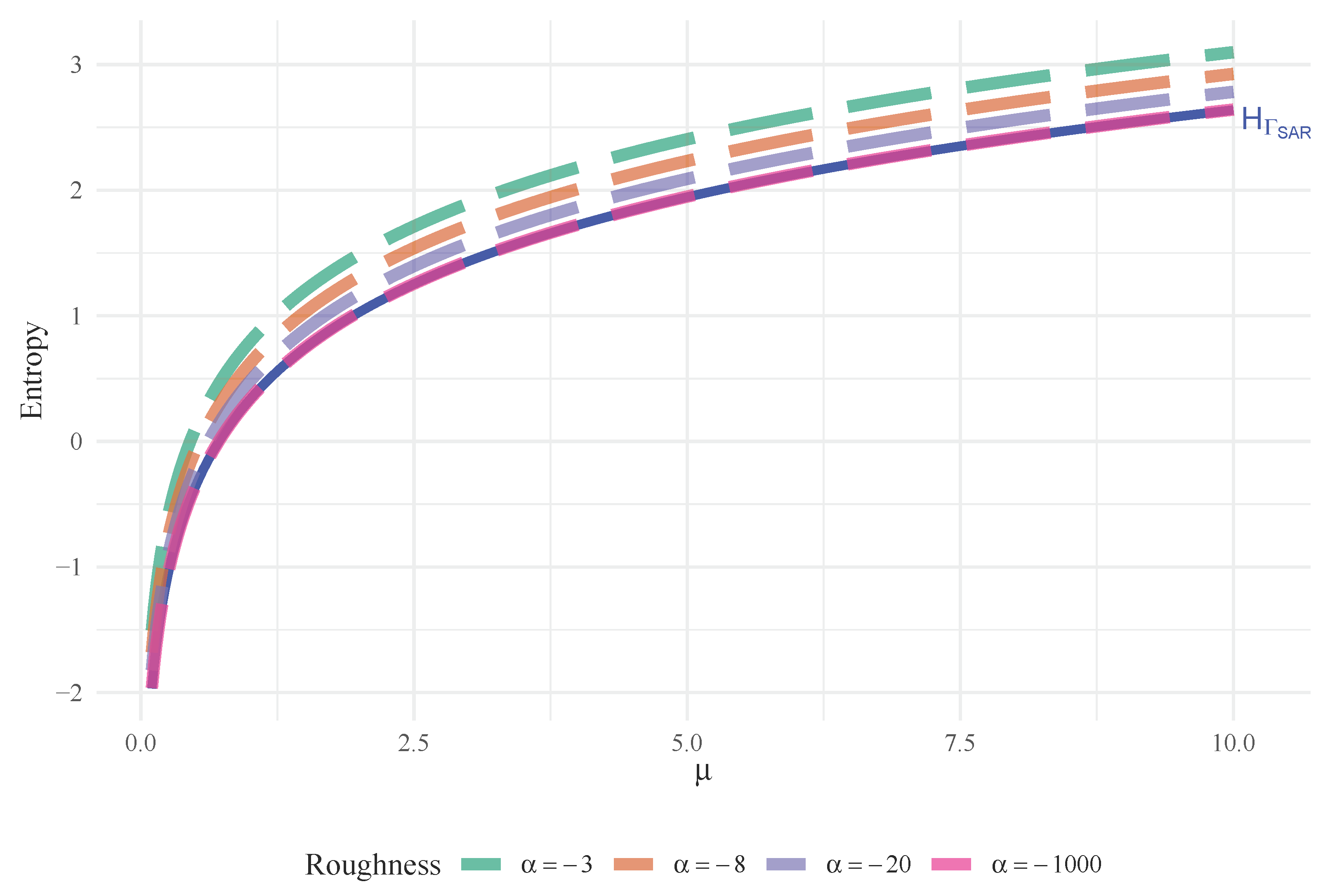
Figure 2.
Bias and MSE of the entropy estimators for the , with .
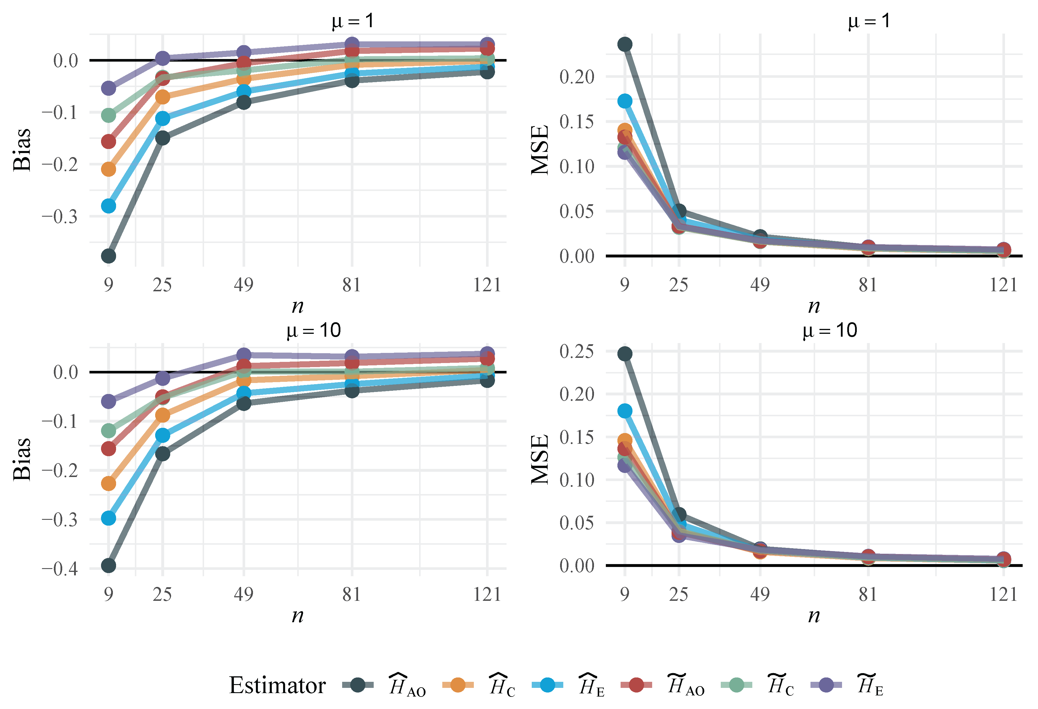
Figure 3.
Empirical densities obtained from test under the null hypothesis.
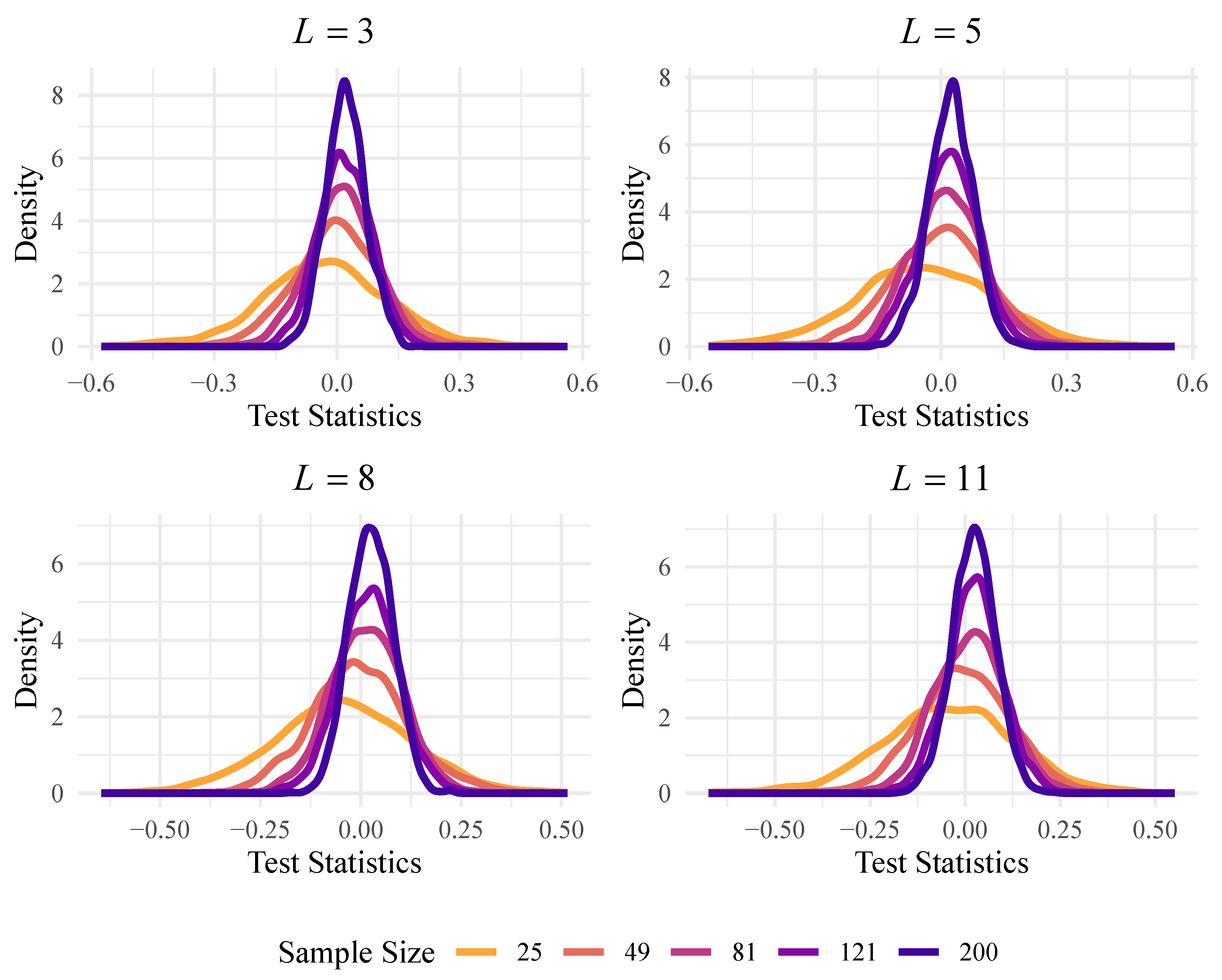
Figure 4.
Normal Q–Q plots for .
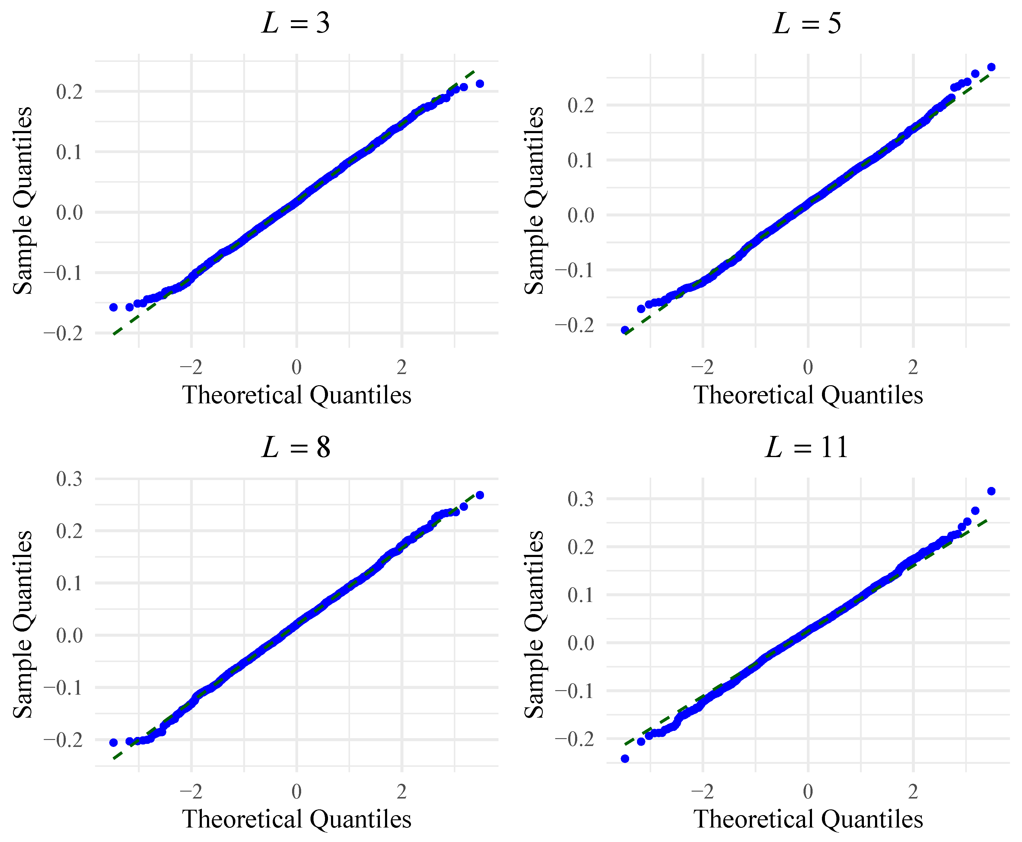
Figure 6.
Goodness of fit plots for evaluating the best distribution with CV data from (under the alternative hypothesis), with , , , and .
Figure 6.
Goodness of fit plots for evaluating the best distribution with CV data from (under the alternative hypothesis), with , , , and .
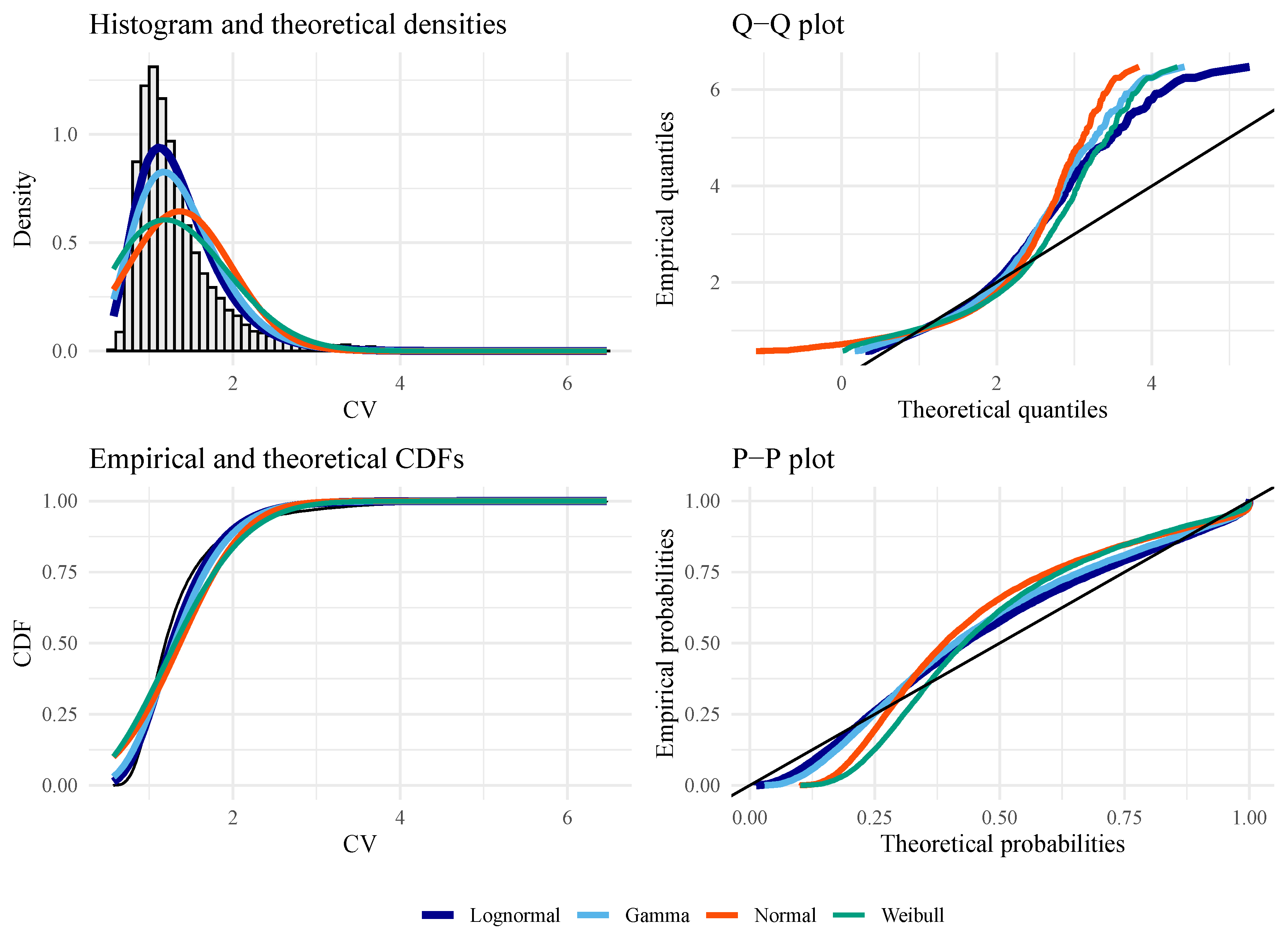
Figure 7.
Goodness of fit plots for evaluating the best distribution with data from (under the null hypothesis), with , , and .
Figure 7.
Goodness of fit plots for evaluating the best distribution with data from (under the null hypothesis), with , , and .
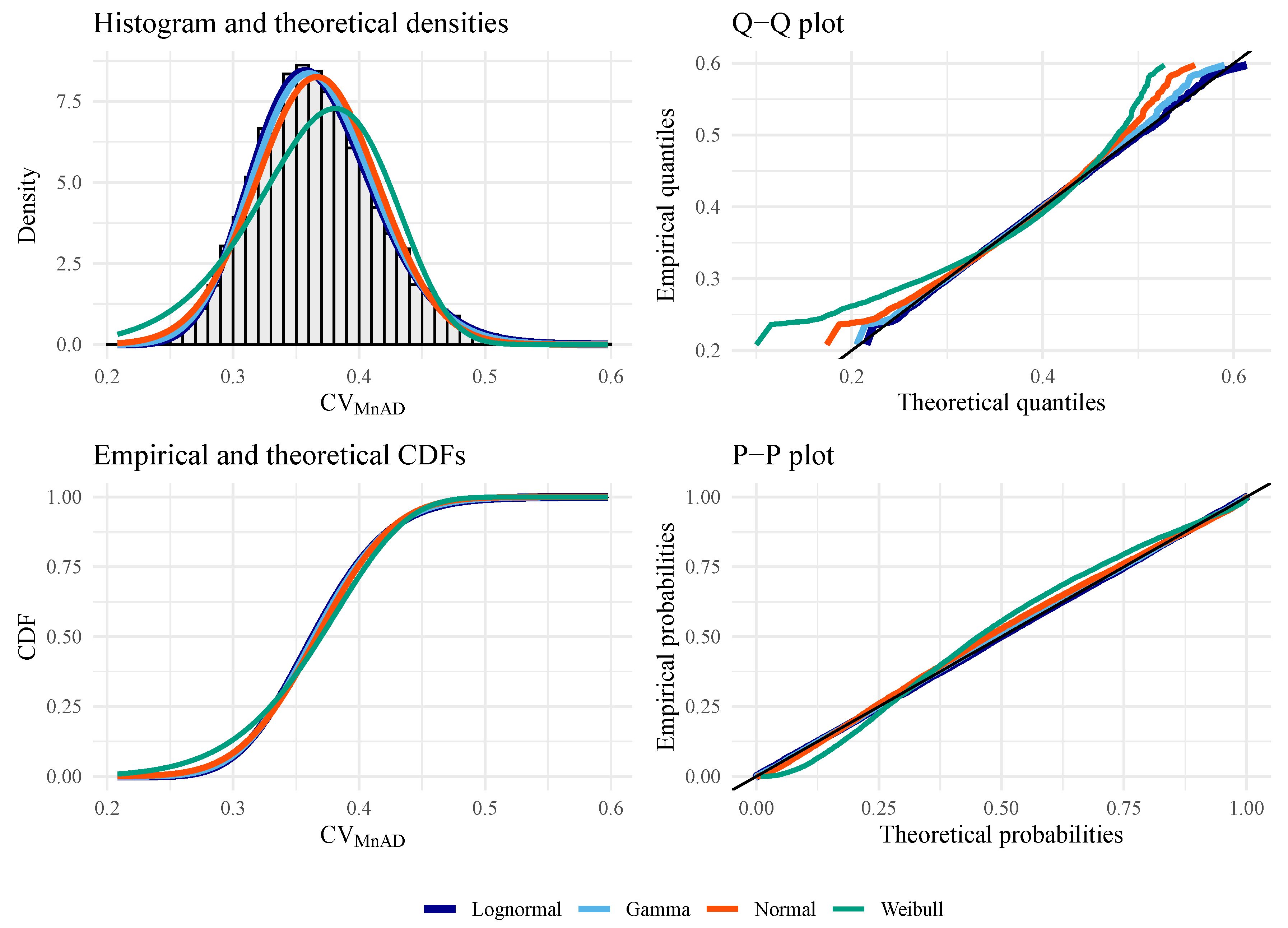
Figure 8.
Goodness of fit plots for evaluating the best distribution with data from (under the alternative hypothesis), with , , , and .
Figure 8.
Goodness of fit plots for evaluating the best distribution with data from (under the alternative hypothesis), with , , , and .
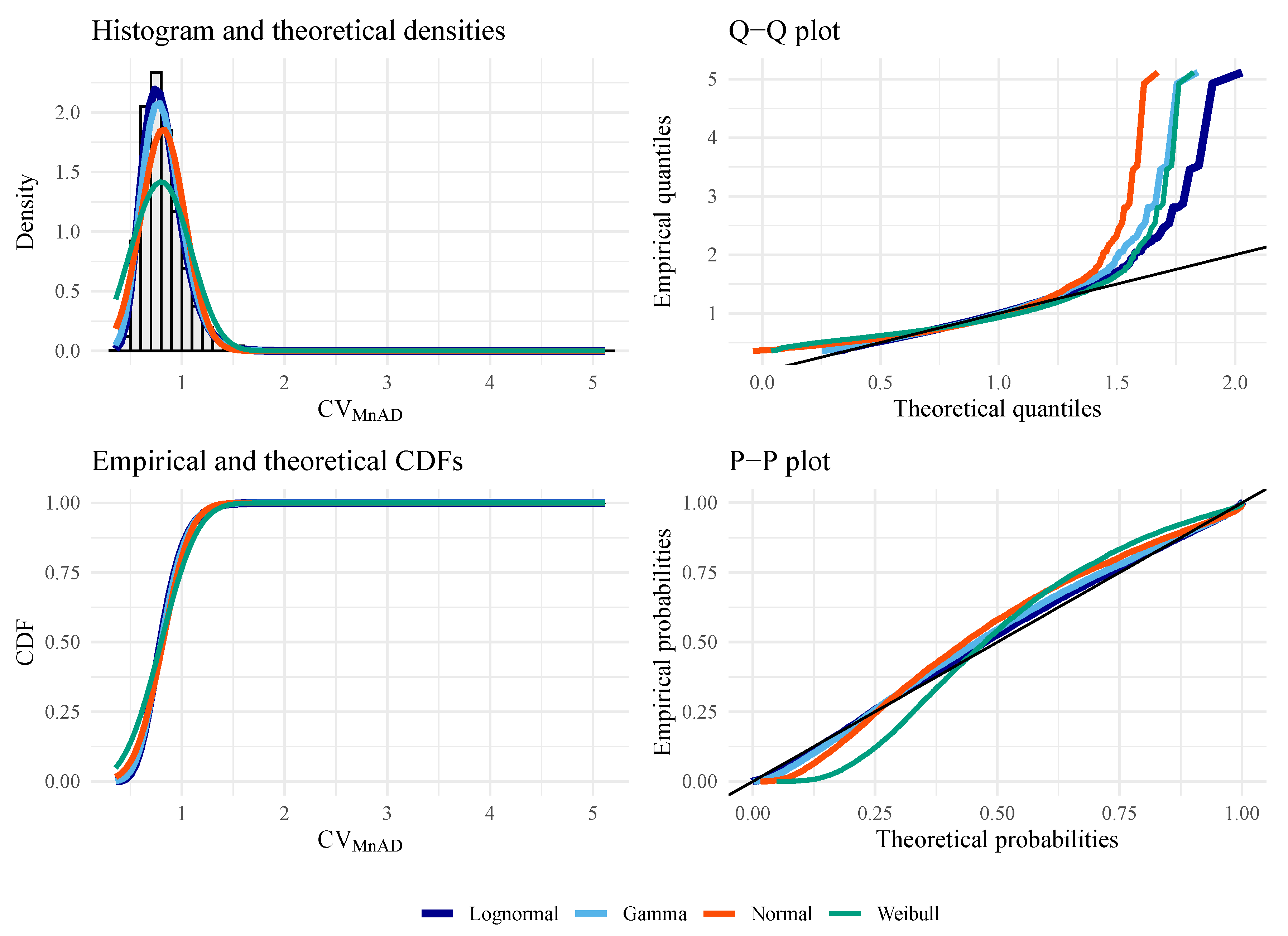
Figure 9.
Synthetic dataset: (a) Phantom. (b) Simulated image, varying and , with .
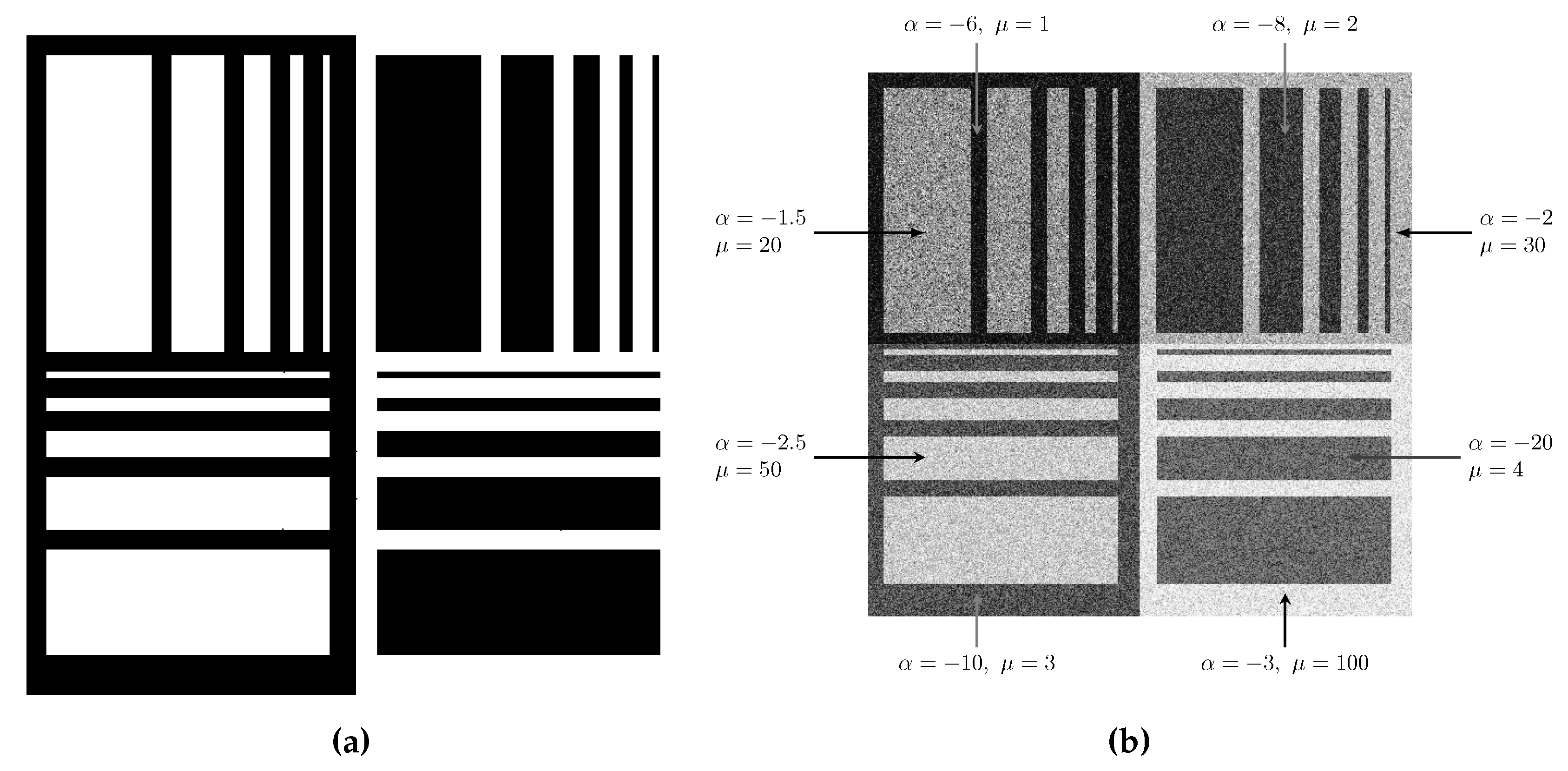
Figure 10.
Results of applying the test statistics: (a) , (b) , and (c) .
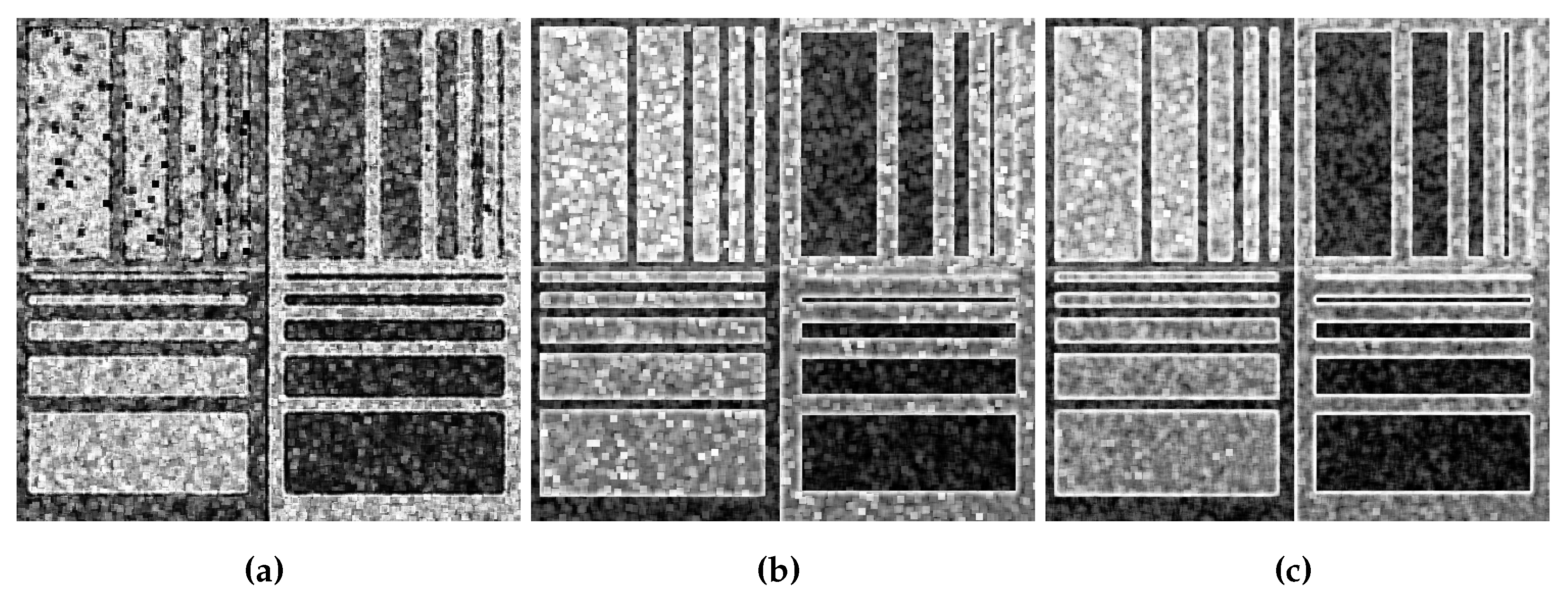
Figure 11.
Map of p-values: (a) , (b) , and (c) .
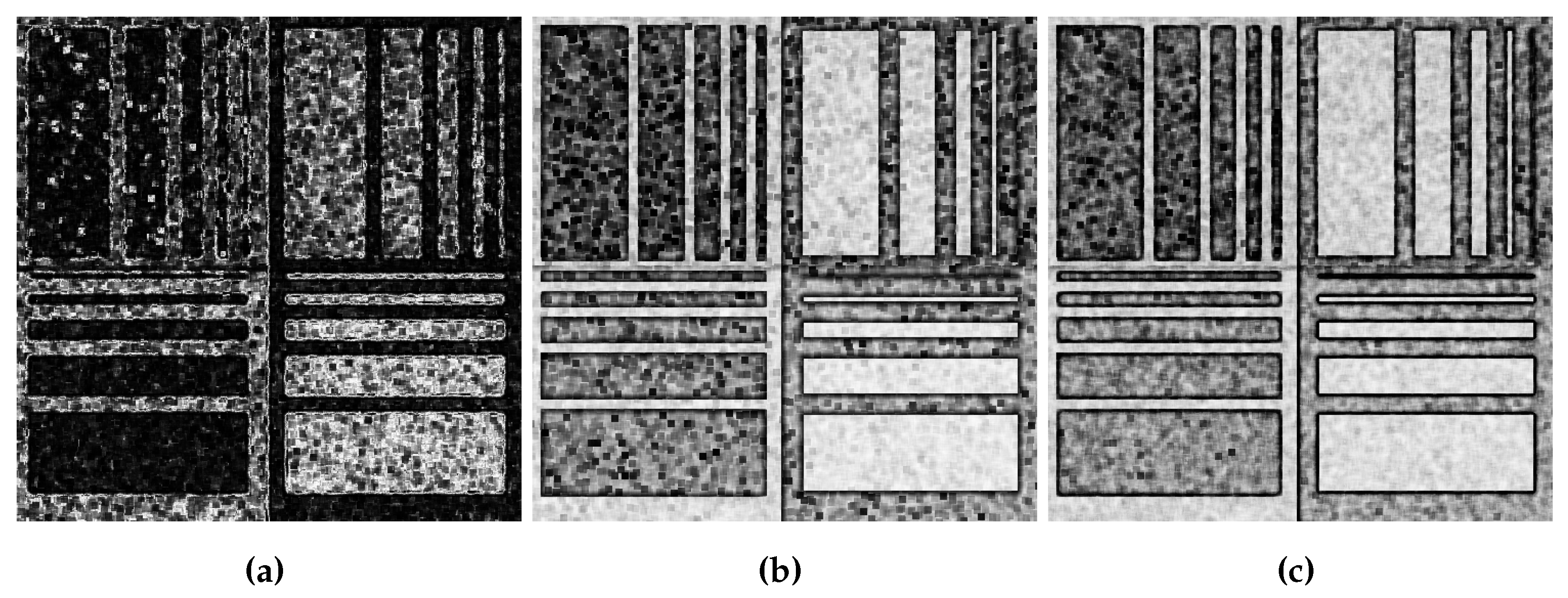
Figure 12.
Results for a threshold of of the p-value: (a) , (b) , and (c) .
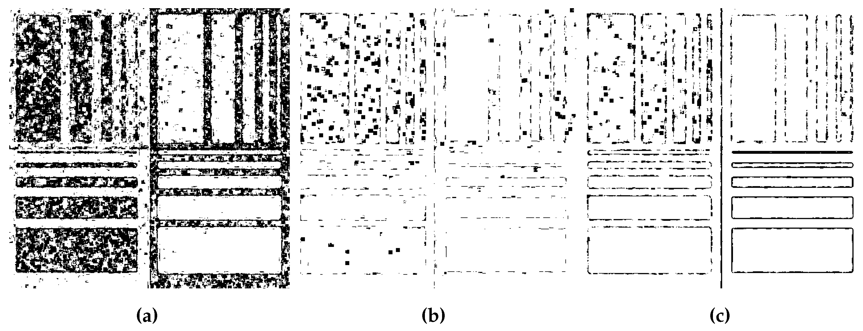
Figure 13.
SAR images: (a) Coast of Jalisco, with . (b) Illinois-Region 1, with . (c) Illinois-Region 2, with .
Figure 13.
SAR images: (a) Coast of Jalisco, with . (b) Illinois-Region 1, with . (c) Illinois-Region 2, with .
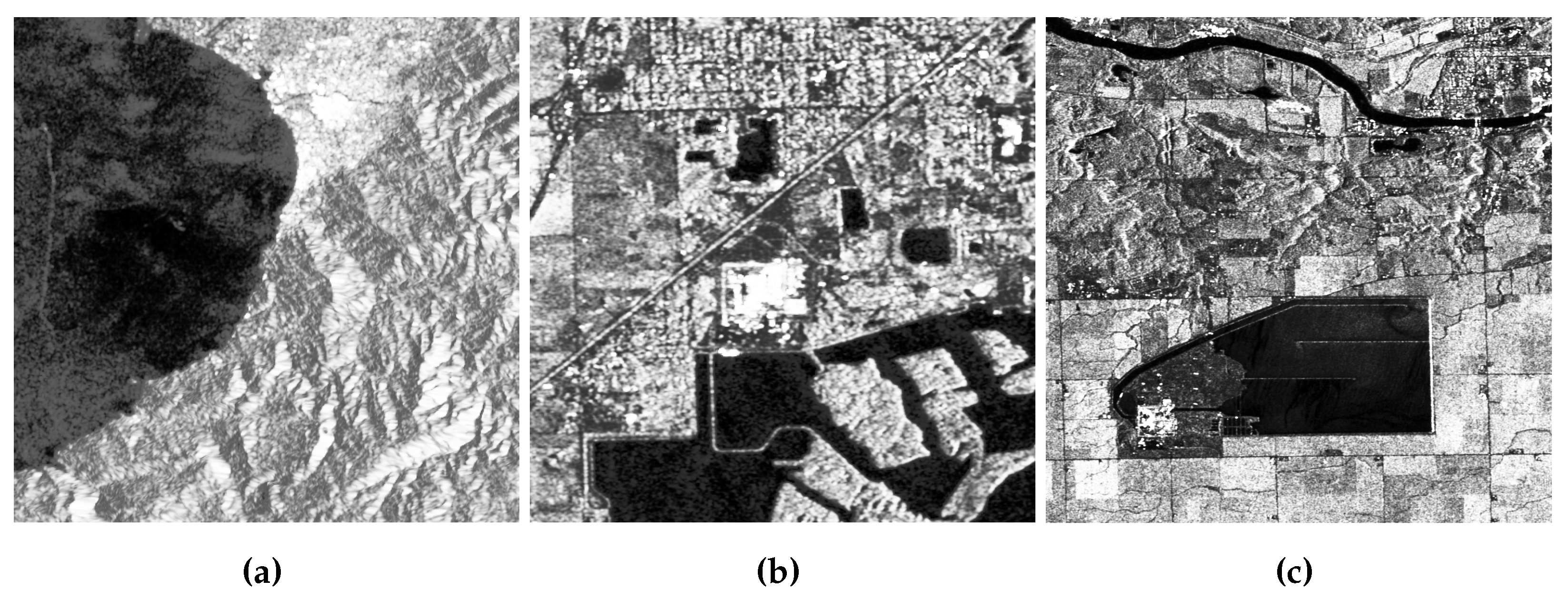

Table 1.
Bias and MSE of the entropy estimators for the , with .
| Bias | MSE | ||||||||||||
| 9 | |||||||||||||
| 1 | 25 | ||||||||||||
| 49 | |||||||||||||
| 81 | |||||||||||||
| 121 | |||||||||||||
| 9 | |||||||||||||
| 10 | 25 | ||||||||||||
| 49 | |||||||||||||
| 81 | |||||||||||||
| 121 | |||||||||||||
Table 2.
Test accuracy and processing time for each bootstrap-improved estimator.
| Estimator | L | n | Time (s) | |
| 25 | 22.53 | |||
| 2 | 49 | 40.35 | ||
| 81 | 63.93 | |||
| 121 | 97.06 | |||
| 25 | 22.25 | |||
| 8 | 49 | 33.42 | ||
| 81 | 50.94 | |||
| 121 | 97.35 | |||
| 25 | 4.66 | |||
| 2 | 49 | 5.55 | ||
| 81 | 6.89 | |||
| 121 | 7.90 | |||
| 25 | 4.81 | |||
| 8 | 49 | 5.43 | ||
| 81 | 6.38 | |||
| 121 | 7.46 | |||
| 25 | 4.61 | |||
| 2 | 49 | 5.19 | ||
| 81 | 6.70 | |||
| 121 | 7.41 | |||
| 25 | 4.74 | |||
| 8 | 49 | 5.35 | ||
| 81 | 6.21 | |||
| 121 | 7.48 |
Table 3.
Descriptive analysis of , with and .
| L | n | Mean | SD | Var | SK | EK | p-Value |
|---|---|---|---|---|---|---|---|
| 25 | |||||||
| 3 | 49 | ||||||
| 81 | |||||||
| 121 | |||||||
| 200 | |||||||
| 25 | |||||||
| 5 | 49 | ||||||
| 81 | |||||||
| 121 | |||||||
| 200 | |||||||
| 25 | |||||||
| 8 | 49 | ||||||
| 81 | |||||||
| 121 | |||||||
| 200 | |||||||
| 25 | |||||||
| 11 | 49 | ||||||
| 81 | |||||||
| 121 | |||||||
| 200 |
Table 4.
Size and Power of the test statistic.
| Size | Power | ||||||
| 25 | |||||||
| 3 | 49 | ||||||
| 81 | |||||||
| 121 | |||||||
| 25 | |||||||
| 5 | 49 | ||||||
| 81 | |||||||
| 121 | |||||||
| 25 | |||||||
| 8 | 49 | ||||||
| 81 | |||||||
| 121 | |||||||
| 25 | |||||||
| 11 | 49 | ||||||
| 81 | |||||||
| 121 | |||||||
Table 5.
AIC and BIC values for evaluating the best distribution with CV data from .
| Criterion | n | Normal | Lognormal | Gamma | Weibull | Inverse Gaussian |
|---|---|---|---|---|---|---|
| 25 | ||||||
| AIC | 49 | |||||
| 81 | ||||||
| 121 | ||||||
| 25 | ||||||
| BIC | 49 | |||||
| 81 | ||||||
| 121 |
Table 6.
AIC and BIC values for evaluating the best distribution with CV data from .
| Criterion | n | Normal | Lognormal | Gamma | Weibull | Inverse Gaussian |
|---|---|---|---|---|---|---|
| 25 | ||||||
| AIC | 49 | |||||
| 81 | ||||||
| 121 | ||||||
| 25 | ||||||
| BIC | 49 | |||||
| 81 | ||||||
| 121 |
Table 7.
AIC and BIC values for evaluating the best distribution with data from .
| Criterion | n | Normal | Lognormal | Gamma | Weibull | Inverse Gaussian |
|---|---|---|---|---|---|---|
| 25 | ||||||
| AIC | 49 | |||||
| 81 | ||||||
| 121 | ||||||
| 25 | ||||||
| BIC | 49 | |||||
| 81 | ||||||
| 121 |
Table 8.
AIC and BIC values for evaluating the best distribution with data from .
| Criterion | n | Normal | Lognormal | Gamma | Weibull | Inverse Gaussian |
|---|---|---|---|---|---|---|
| 25 | ||||||
| AIC | 49 | |||||
| 81 | ||||||
| 121 | ||||||
| 25 | ||||||
| BIC | 49 | |||||
| 81 | ||||||
| 121 |
Disclaimer/Publisher’s Note: The statements, opinions and data contained in all publications are solely those of the individual author(s) and contributor(s) and not of MDPI and/or the editor(s). MDPI and/or the editor(s) disclaim responsibility for any injury to people or property resulting from any ideas, methods, instructions or products referred to in the content. |
© 2024 by the authors. Licensee MDPI, Basel, Switzerland. This article is an open access article distributed under the terms and conditions of the Creative Commons Attribution (CC BY) license (http://creativecommons.org/licenses/by/4.0/).
Copyright: This open access article is published under a Creative Commons CC BY 4.0 license, which permit the free download, distribution, and reuse, provided that the author and preprint are cited in any reuse.