Submitted:
30 April 2024
Posted:
02 May 2024
You are already at the latest version
Abstract
Deterministic simulations using the SWAN model were conducted along a stretch of the Tietê-Paraná waterway in the Ilha Solteira dam reservoir, São Paulo, Brazil, to assess the water waves generated by winds. Simultaneously employs a probabilistic metamodeling approach (PCE) and Sobol indices, to quantify uncertainty of the five involved physical parameters (wind velocity and direction, bottom friction (JONSWAP), whitecapping and depth-induced breaking index). In the deterministic part, Janssen’s formulation yielded the most successful and accurate estimations of wave heights. Probabilistic analysis underscored the importance of wind data and the whitecapping parameter in model calibration, with a significant influence of wind speed indicated by Sobol indices. The results not only refined the model calibration process, but also allowed the creation of contour maps for wave height and period that offer practical pre-project applications. This work advances understanding of wind wave hydrodynamics deterministically and probabilistically, with good concordance and performance indices compared to field data, despite being scarce.
Keywords:
Wave modeling
; Wind waves
; SWAN model
; Metamodeling
; Sobol’s index
; Uncertainty quantification
1. Introduction
The analysis of hydrodynamics in dam reservoirs is a topic of growing global importance, with significant implications for navigation safety, environmental preservation, and project planning, especially in the context of hydroelectric power plants. Although hydrodynamic understanding in open environments, such as coastal zones, has been extensively studied, the investigation in closed enclosures, such as reservoirs, still faces challenges due to the scarcity of field data and in obtaining the database (e.g. winds and bathymetry) necessary for the calibration and validation of numerical modeling [1-13].
The safety of inland navigation and the mitigation of significant erosion phenomena in lake environments, enclosed areas such as dam reservoirs, require an accurate estimate of the action of wind waves (wave force/energy) on the banks of the reservoir and on structures, whether fixed (such as dams, retaining walls, mooring structures, and guide walls) or mobile (such as the vessel itself).
For these reasons, it has become increasingly important to develop methodologies and tools capable of forecasting and monitoring wind waves in reservoirs and stretches of waterway. In this sense, controlling the level of agitation of the reservoir's free surface and its effects on fixed or mobile structures and banks is, in fact, an essential element in building a basis for a future warning system [8, 14-21].
To develop these methodologies and tools, numerical models are very useful for assessing the generation and forecasting of wind waves. One of the most widely used tools is the SWAN (Simulating Waves Nearshore) model, proposed by Booij et al. [2,3], which can simulate the generation, propagation and dissipation of waves in coastal regions and inland waters, based on wind kinetics and the wave action conservation equation. Although very useful, numerical models such as SWAN require validation and calibration using empirical data, obtained from measuring stations (floats).
In this context, Gruijthuijsen [1] presented a validation of the SWAN model using field data from Lake George, Australia. This lake is considered shallow, with a practically constant depth of 2.0 m. Using data obtained from eight floats along the longest axis (north-south) of the lake and three studies of case with constant wind speeds (stationary mode), the author demonstrated the applicability of the SWAN model in restricted waters, evaluating and calibrating different parameters and formulations.
Along these lines, Jin & Ji [22] also used the SWAN model in the shallow waters of Lake Okeechobee in Florida (average depth 3.0 m), using two sets of wave height and wind data: 1) data from 6 days in 1989 to calibrate the model; and 2) data from 6 days in 1996 to validate the model. The analyses showed good agreement between the measured and simulated data, as well as a solid correlation between wave height and wind field.
The SWAN model was also used by Moeini & Etemad-Shahidi [23] to analyze wind waves in Lake Erie, North America. The researchers considered wind dynamics and a complex bathymetry varying up to 58 m in depth, with an average depth of 19 m. The study data was collected for 276 hours over eleven and a half days. Among the main results, the researchers highlight that the SWAN model showed a good ability to predict variations in 𝐻𝑠 (significant wave height) and 𝑇𝑝 (peak period) when the wind suddenly changes direction and speed.
Mao et al. [4] used a 10-year database of wind speed and significant wave height to check the sensitivity of the equations and parameters of the SWAN model using unstructured meshes and then calibrate it. Good agreement was found between the numerical and field data.
The Brazilian research group has been working on the reservoir of Ilha Solteira’s / SP (Brazil) reservoir since 2002 and has produced a number of studies, including Vieira et al., [24], Vieira [25], Mattosinho [26], Mattosinho, Maciel and Vieira [20], Mattosinho et al, [8] and Mattosinho, Ferreira and Maciel [27], based on previous versions of the SWAN model, obtaining promising statistical index, but emphasizing the continuous need for improvement in terms of calibration. A few additional endeavors are underway in Brazil, notably around Lagoa dos Patos / RS, where the SWAN model has been consistently underestimating observed data and can be verified in Lemke et al., [31], Simão [32], Lemke et al., [6, 33], Lima et al., [34], Marinho et al. [7] and Lemke et al. [35].
This study focuses on the application of the third generation SWAN (Simulating Waves Nearshore) model to analyze wind waves in a strech of the Tietê-Paraná Waterway, located in the reservoir of the Ilha Solteira Hydroelectric Power Plant / SP, Brazil. The choice of this scenario is justified by the economic and environmental importance of the region, highlighting the need to understand wind wave phenomena and their effects.
This research differs from previous work by the research group, mainly by adopting version 41.31 of the SWAN model on an open platform, where the simulations are carried out based on a persistence level of 99.5% of 𝐻𝑠, using more refined meshes (ensuring GCI: Grid Convergence Index); physical analysis of the main parameters involved in wave propagation and the adoption of hourly averages for wind data (speed and direction). In addition, this work takes a pioneering approach to metamodeling and uncertainty quantification for the study area.
The aim of this article is therefore to explore the hydrodynamics of wind waves in the Ilha Solteira DAM lake, using a deterministic approach with the SWAN code and a probabilistic approach to quantify uncertainties, including the development of a Polynomial Chaos Expansion (PCE) metamodel via regression [36]. The aim is to determine the sensitivity and quantify the uncertainties of the physical parameters involved in the generation and propagation of waves, in a way that has not yet been explored, contributing to multidisciplinary projects and studies aimed at improving social, economic and safety conditions, especially for navigation and environmental preservation.
2. Materials and Methods
This section presents a description of the study area, the methodological procedures for the numerical simulations carried out in the SWAN 41.31 model, as well as the probabilistic methods applied to analyze the physical parameters involved in the dynamics of wind-generated waves.
2.1. Description of the Study Area
The research focuses on the reservoir of the Ilha Solteira Dam (Figure 1), part of the Urubupungá Complex, the sixth largest hydroelectric complex in the world. Located approximately 5 km from the city of Ilha Solteira, a municipality in the northwest of the state of São Paulo, the reservoir has an important role in the Tietê-Paraná waterway and on the MERCOSUL (Southern Commom Market) trade route.
In climatological terms, the region is classified as a savannah climate (Koppen Aw), with rainfall predominantly in summer. The winds, which are mostly moderate (with an average wind of 5 m/s), can reach speeds of over 10 m.s-¹, with extreme gusts of 33.3 m/s (120 km/h) recorded in exceptional situations [37, 38]. The prevailing wind direction is northeast, influencing the formation of waves along the navigation route [25].
The reservoir of the Ilha Solteira Dam is geographically located at a latitude of 20º25'58" south and a longitude of 51º20'33" west, with an altitude of approximately 335 meters. Strategically located at the confluence of the Tietê and Paraná rivers, on the border with the state of Mato Grosso do Sul, it covers an area of 1,195 km², with a length of 5,605 meters according to CESP (former Energy Company of São Paulo).
With a maximum effective fetch of around 22.5 km in a north-easterly direction, the study area stands out as a vital part of the Tietê-Paraná waterway, essential for commercial transportation in the MERCOSUL region. The reservoir draws water from a vast area of 375,460 km², with operating levels ranging from 323 to 328 meters above sea level.
The field data used in this research was obtained during the ONDISA project (ONDas no reservatório de Ilha SolteirA) [28, 29]. Wind speed and direction were measured by a 2D sonic anemometer positioned 1.2 m above water level. Pressure data was measured by a Druck PDCR 1830 pressure sensor (for up to 50 psig, 0.06% full scale nonlinearity, equipped with a 150 m power cable) positioned 1.0 m below the water level. Further details of the field work are presented in Maciel et al., [39]; Vieira [25]; Mattosinho et al., [40] and Mattosinho et al., [8].
2.2. Numerical Modeling
Numerical simulations were carried out using the SWAN model (version 41.31) in its standard version, following the guidelines of the development team [40]. The methodological procedures for the deterministic approach are shown in Figure 4.
A notable feature of SWAN is its flexibility in modeling different scales, from coastal areas to large ocean basins. This versatility, combined with the ability to simulate complex interactions between waves and other coastal processes, gives SWAN an outstanding position in the numerical modeling of hydrodynamic phenomena.
SWAN uses rectangular meshes for spatial discretization, employing a spectral approach in which space is divided into elementary cells with constant spacing and . This offers constant directional resolution and constant relative frequency resolution This logarithmic frequency distribution is essential for an accurate representation of wave conditions. The wind field does not depend on depth ().
In the calculation phase, the model uses the spectrum action balance equation, which is a function of the action density, where is the relative frequency, is the direction of the wave and is the energy density. Formulated in Eulerian coordinates, the action spectrum equation is given by Equation 1.
In summary, the left side of Equation 1 represents the kinematic component of the model, while the right side represents the source/sink term. Term 𝑆𝑡𝑜𝑡 is then expressed by Equation 2.
These six terms for wave energy sources and sinks represent wave growth by wind input, non-linear wave energy transfer through triple and quadruple wave interactions, wave decay due to whitecapping, bottom friction and depth-induced wave breaking, respectively.
On the deterministic side, wave heights are simulated using data from the ONDISA project referring to January 2011. The comparison between the simulated and measured results focuses on the significant wave height (𝐻𝑠), considering the limited data available, such as the wave period. The appropriate resolution of the SWAN model mesh is assessed using the Grid Convergence Index (GCI) method [42, 43] for 250 m, 150 m and 100 m resolution meshes, Table 1. The frequency band considered is 0.04 to 1.00 Hz with 144 intervals and the nautical convention is used.
Five statistical indices [45] are used to compare the numerical results with the experimental ones. All the analyses are carried out using data from the monitoring station and results from various cases simulated using the SWAN model, varying the formulations for wave generation, friction in the wind speed field, background friction, whitecapping, as well as checking the activation and deactivation of the diffraction and wave breaking index parameters. Wind data from January 2011 was used for this purpose.
- -
- Root Mean Square Error (𝑅𝑀𝑆𝐸) given by Equation 3, the lower its value, the greater the agreement between the numerical and experimental results.
- -
- Willmott's Concordance Index () (Equation 4) determines the accuracy of the method and indicates how far the estimated values are from the observed values. This index ranges from 0, for no agreement, to 1, for perfect agreement.
- -
- Dispersion Index ( represents a measure of relative error (Equation 5).
- -
- represents the systematic deviation from the actual value (Equation 6).
- -
- Person's Correlation Coefficient () given by Equation 7.
- -
- Performance Index () expressed by Equation 8.where:
: dada observed via monitoring station
: average of observed data
: simulated data via Swan
: average of simulated data
: amount of data
2.3. Metamodeling
On the probabilistic side, the procedures carried out are shown in Figure 5.
In the initial phase, the sample number is determined by analyzing the convergence of the significant wave height results in relation to the input random variables, namely: wind speed and direction, JONSWAP bottom friction coefficient, induced wave breaking index and whitecapping coefficient from Komen's formulation. The values and probability distributions are established considering the principle of maximum entropy [46]. Probabilistic methods for propagating uncertainties, such as PCE, are applied, and the global sensitivity is evaluated by Sobol Indices [47] of first and second order to determine the percentage influence of each random variable using the UQLab library [36], a platform recognized for its effectiveness in the comprehensive analysis of uncertainties. In fact, to strengthen the reliability and robustness of the SWAN simulations, we used Uncertainty Quantification (UQ) that is important for validating and improving models, especially when the data is scarce or subject to variations.
Given a mathematical model that has independent input parameters grouped into an input vector and a scalar output , we have (Equation 9):
It’s possible to define in the decomposition into sums of different dimensions [48]. To simplify the notation of this example, all the following equations will assume that the input variables are uniform and that the support of the input set is . Thus, is defined by Equation (10).
where all the sums in the expansion can be calculated by means of recursive integrals, the first term is constant and equal to the expected value (Equation 11):
The other terms represent the conditional mean values for the parameters and ().
In this context, the Sobol decomposition can be defined in terms of conditional variances [47]. In this way, first-order Sobol indices are obtained, which measure the additive effect of each input individually in relation to the total variance (Equation 12). The interaction effects between the inputs, on the other hand, are used as a second-order index (Equation 13).
The Sobol indices calculated by PCE can be found in Crestaux, Maitre and Martinez [49] and Palar et al. [50]. The first-order Sobol indices, by quantifying the individual influence of each input variable, reveal the proportion of the model's total variance attributed to each variable. These indices are essential for identifying the variables that have the greatest single impact on the model's performance, providing an in-depth understanding of the relative importance of each factor.
On the other hand, second-order Sobol indices go further, considering interactions between pairs of input variables. By analyzing the contribution of interactions between two variables to the total variance of the model, these indices provide a more comprehensive view of the relationships between variables. This approach is valuable for understanding how combinations of variables influence the behavior of the system, highlighting patterns and synergies that may not be evident when analyzing only the variables in isolation.
Subsequently, the PCE technique is implemented to build a substitutive model that approximates the behavior of the original SWAN model. This is achieved by developing multivariate polynomials, considering the input random variables and their corresponding coefficients. The PCE method, operated using the UQLab library [51] in MATLAB, provides a substantial reduction in processing time while maintaining the accuracy of the results. The substitutive model is validated using the 80/20 method in combination with the bootstrap technique with 1000 iterations.
Finally, Global Sensitivity Analysis (GSA) is conducted to quantify the contribution of each input variable to the results of the SWAN model [52, 53]. The Sobol Indices method is adopted, allowing the total variance of the system's response to be broken down into the individual and joint contributions of the input variables. The first order and second Sobol Indices are calculated directly from the substitutive model constructed. GSA in conjunction with UQ emerges as a unique approach to elucidating the relationships between the model's input and output variables.
It should be noted that the methodology presented provides a comprehensive analysis, integrating both deterministic and probabilistic modeling, with a view to gaining an in-depth understanding of the dynamic behavior of waves, taking into consideration the uncertainty associated with the input parameters.
3. Results and Discussion
This section presents the results of the deterministic and probabilistic approaches. Firstly, a mesh sensitivity analysis was carried out using the Grid Convergence Index (GCI) method.
The GCI method is widely used in the literature to estimate uncertainties and errors in computational fluid dynamics. The final value, GCI, is given as a percentage and there are no studies in the literature that define the maximum admissible value, except for the norm ASME V&V 20-2009 [43]. As such, GCIs of less than 5% are considered adequate. Table 2 shows the data used to determine the GCI. The procedures for determining this can be found in norm ASME V&V 20-2009 in item 2-4.1. For the calculations, the wind speed is considered constant.
Having verified the applicability of the 150 m resolution mesh, it was decided to use the 100 m resolution mesh, which is also in the range allowed in the SWAN model user manual, between 50 and 1000 m [44] to carry out the physical analyses in the intermediate and shallow water region to verify the model's sensitivity in the region. It should be noted that analyses for wind speeds of 10, 15 and 20 m/s showed GCI percentage values even lower than 1.65%.
After that, we proceeded to analyze the field data in relation to the SWAN model results for the monitoring station, which is in deep water (relative depth ) [54], using the 1000 m mesh due to its good statistical performance compared to the others, as shown in Table 3.
These results reinforce the theory that bathymetry can contain imperfections, which become more evident in more refined meshes. This is due to the interpolation between the nodes, which in the 1000 m mesh ends up generating a bathymetric mesh with a smoother bottom.
The meticulous approach adopted in this research, integrating field measurements, deterministic modeling, and probabilistic analysis, revealed substantial knowledge about wind waves in enclosed areas, with a focus on the Ilha Solteira reservoir, for a scenario of scarce field data. In sections 3.1 and 3.2, we present and discuss the results obtained from both the deterministic and probabilistic approaches, highlighting the significant contributions to understanding the phenomenon in question.
3.1. Deterministic Approach
On the deterministic side, the Janssen formulation for wave generation and the whitecapping phenomenon showed superior performance in modeling the waves in the reservoir (Figure 5, Table 4 and Table 5). The statistical analysis revealed notable improvements compared to previous work by the research group (Vieira, 2013 [25]; Mattosinho et al. 2022 [8]), marking a significant advance in the representation of the specific hydrodynamic conditions of Ilha Solteira. Although the ideal calibration, with a determination index () of over 95% has not been fully achieved, the progress made is significant.
Modeling in previous work by the research group was carried out using Komen's formulations for wave generation and whitecapping effects, and this work shows that Janssen's formulation provides better statistical results.
Figure 6.
Analysis of third-generation equations (GEN3) of the swan model, alongside significant wave height () data from pressure sensor and wind speed collected by anemometer at the monitoring station for the period of January 2011.
Figure 6.
Analysis of third-generation equations (GEN3) of the swan model, alongside significant wave height () data from pressure sensor and wind speed collected by anemometer at the monitoring station for the period of January 2011.

It is worth mentioning that the changes for the modeling and analysis are made only to the parameters presented. Except for the JONSWAP bottom friction coefficient () the other variables and parameters of the SWAN model have been maintained in accordance with the standard recommended in the manual. In addition, the Komen wave generation formulation is adopted in the case study for the effect of whitecapping formulations presented in Table 5.
It should be noted that the physical wave generation formulation ST6 (GEN3 ST6) of Rogers et al., (2012 [55]), as investigated in the work of Sapiega, Zalewska, Struzik (2023 [12]), stood out as a viable alternative for the Southern Baltic Sea region. However, for the case of the Ilha Solteira dam reservoir, Janssen's formulation for wave generation and whitecapping proved to be more suitable, highlighting the need for careful evaluation of formulations for different study locations.
The SWAN team [41] state that the “ST6” source term package was implemented in an unofficial version of SWAN starting in 2008 and initial development was documented in Rogers et al. (2012). At the time, it was referred to as “Babanin et al. physics” rather than “ST6”. ST6 was implemented in the official version of WAVEWATCH III R(WW3) starting in 2010, and this implementation was documented in Zieger et al., (2015). Since 2010, developments in the two models have largely paralleled each other, insofar as most notable improvements are implemented in both models. As such, the documentation for WW3 (public release 24 Chapter 2 versions 4 or 5) is largely adequate documentation of significant changes to the source terms in SWAN since the publication of Rogers et al. (2012).
Analyzing current works, such as those by Nikishova et al., (2017 [5]) and Zhang et al., (2023 [11]), the critical influence of the wind field as the main factor in wave generation is evident. This corroborates the need to verify various physical models, including the whitecapping parameter and coefficient, to achieve a more accurate calibration and replication of field data. Zhang et al. (2023 [11]) state that the whitecapping coefficient in the formulations must be calibrated to adjust the model's results curve to the field results.
Given the foregoing, studies analyzing the values of the whitecapping coefficient for the Komen and Janssen formulations should still be carried out for the case of Ilha Solteira to improve the calibration of the model, which currently has a performance index of 70% (Table 4 and Table 5). Zhang et al. (2023 [11]) proposed, for example, a dissipation coefficient for whitecapping in the Komen equation of 3,25 × 10⁻⁵ for the validated model, a value substantially different from that recommended in the SWAN model manual, which is 2,36 × 10⁻⁵. This highlights the significant influence of this coefficient on calibration in each study area and justifies continuous improvement and refinement.
3.1. Probabilistic Approach
The case study consists of the analysis of five random variables chosen due to the high recurrence of mentions of their relevance in research involving calibration of the SWAN model. Speed (𝑣𝑒𝑙) and direction (𝑑𝑖𝑟) of the wind, the JONSWAP bottom friction coefficient (), the induced wave breaking index ( where is local depth) and the whitecapping coefficient from the standard formulation (𝑐𝑑𝑠𝑤).
The input variables, wind speed and direction, were taken from the ONDISA Project database, covering the period from October 2010 to March 2011. In this context, the most appropriate maximum entropy probability distribution for the field data was analyzed using the Python programming language.
It was found that the wind direction fits the uniform distribution, while the wind speed fits the Weibull distribution, as shown in Figure 7. Where is the Weibull probability distribution function, is the shape factor and is the scale factor. This distributional fitting process is crucial for the subsequent stages of probabilistic modeling.
The other variables were considered to have a uniform probability distribution due to the unavailability of field data and were considered to have maximum entropy. Therefore, the maximum and minimum values to be used as supports were checked in the literature. The exception was the whitecapping coefficient, which was a 10% variation around the standard value, as Nikishova, et al., (2017 [5]) proceeded. Table 6 shows the support values for the variables. To guarantee the replicability of this study, "seed = 1102" was used.
Samples of 100, 300, 500, 700, 1000, 1500, 2000 and 3000 random data were generated, and the input files were created and executed in the SWAN model in the same way as in the deterministic model to obtain the results for significant wave height (𝐻𝑠). Once the convergence of the samples had been analyzed, the sample with 3000 data was adopted for the case study.
The significant contribution of this research was the quantification of uncertainties and the analysis of Sobol indices, an approach notably scarce in the existing literature on wind waves in dam reservoirs. The results highlighted the sensitivity of the SWAN model to different physical configurations, underlining the importance of considering different models for a more accurate calibration.
The first check carried out refers to the histogram containing the model's true outputs and the predictions of the grade 8 PCE (Figure 8), which shows the good behavior and replication of the PCE. Other points of interest are the verification of the Sobol indices of 1st order (Figure 9), 2nd order (Figure 10) and the correlation and determination coefficients between these values (Figure 11), which show excellent behavior.
The observation of a significant influence of the speed variable (𝑣𝑒𝑙) compared to the other variables, as evidenced by the first-order Sobol indices, is consistent with the sensitivity analysis carried out. Given that the sum of the first-order Sobol indices is less than 1, these results suggest that the total variation in the model cannot be completely attributed to the independent variations of each input variable. There are therefore other variables not yet dealt with in this article which may interfere with the results.
In this context, speed emerges as the main contributor to variations in the model's results, accounting for approximately 96% of the total influence. The low contribution of the other variables, such as direction (𝑑𝑖𝑟 ≅ 2%), bottom friction coefficient (), induced wave breaking index (𝑔𝑎𝑚𝑚𝑎), and whitecapping coefficient of the standard formulation (𝑐𝑑𝑠𝑤), is consistent with the observation of negligible influence. This suggests that these variables have less impact on the fluctuations and behavior of the modeled system, corroborating the results of the sensitivity analysis.
The unequal distribution of importance between variables highlights the need to focus on more influential variables, such as speed, when optimizing model performance or identifying key areas for intervention or improvement. This conclusion reinforces the usefulness of Sobol indices as a valuable tool for identifying the relative contribution of input variables in complex models, aiding interpretation, and informed decision-making.
These results are in line with relevant studies, such as those by Nikishova, et al., (2017 [5]), Zhang et al., (2023 [11]) and Sapiega, Zalewska, Struzik (2023 [12]), among others, which point to wind data (speed and direction) as the main variables in modeling and their sensitivity in calibrating the model to real cases in the field, as observed in the deterministic approach.
It is worth noting that the whitecapping parameter is also considered to be of great importance in the calibration of the SWAN model [11], however, in the analyses presented so far, the influence of the whitecapping coefficient of the standard formulation was not observed. To investigate the influence of this parameter in relation to the others considered, the simulation is run in a similar way to the previous one for 3000 data points with a constant speed of 5 m/s and NE direction (northeast = 45º), which are the prevailing winds data in the region (Figure 12, Figure 13 and Figure 14).
There is a greater dispersion in the data and a slight reduction in the correlation and determination coefficients compared to the previous case. However, despite these results, it can be said that the modeling is adequately represented by the PCE.
In this scenario, the whitecapping coefficient of the standard formulation (𝑐𝑑𝑠𝑤) has a significant 1st order Sobol index, reaching 97%. The induced wave breaking index (𝑔𝑎𝑚𝑚𝑎) is 2.4%, while the background friction coefficient () shows a reduced magnitude when we consider wind speed and direction as constant. This set of results can be interpreted in the light of existing literature, indicating that the most impactful parameters and equations in hydrodynamic modeling of closed environments, such as dam reservoirs, are concentrated in the wind data (speed and direction) and in the whitecapping formulation, whose coefficient, as indicated by Zhang et al. (2023 [11]) must be calibrated for the specific wind field used in the modeling.
On the probabilistic side, we confirmed the empirical knowledge of the importance of wind data and the whitecapping parameter in modeling and calibration. Despite the lack of field data, contour maps for significant wave height and mean wave period were generated from the results of the simulations (Figure 15 and Figure 16), providing information for practical applications in preliminary projects in the region, such as those for navigation, fish farming and environmental protection. We emphasize that the maps are in line with the physics of the problem and previous estimates, such as those pointed out by Vieira (2013 [25]) and other productions by the research group.
It could be observed that the wave heights (𝐻𝑠) are greater than 0.4 m if the wind speed is greater than 8 m/s in the NE direction. In this case, the average period is over 0.86 s, with an average of 1.33 s. It should be noted that the prevailing wind speed in Ilha Solteira is moderate, around 5 m/s [27]. In extreme cases of strong gusts, as occurred in 2010 [37, 38], the wind speed can exceed 33 m/s (120 km/h).
To verify the good physical replication in the modeling, the percentage of occurrence of wind direction data in each direction of wave propagation (16 intervals) can be analyzed for the data set (Figure 17), where the ranges in the order of 45° (NE) and 315° (NO) show the highest occurrence.
The NE direction stands out as dominant in the simulated data, just as it did in the field data. As for the NO direction, we hypothesize that its high occurrence is due to the geometry of the lake and wave reflection at the point under analysis, which is the monitoring station relatively close to the shore. The same phenomenon is observed when analyzing the peak direction (Figure 18).
Turning to the analysis of the mean absolute and peak periods of the numerical results, we can see that they are in good agreement with the wind data (Figure 19 and 20). For the data set, the mean absolute and peak periods are 1.3 s and 1.7 s, respectively. This indicates the model's good performance for the case study.
The results of this study not only provide a more refined calibration of the SWAN model for the specific case of Ilha Solteira, but also suggest more assertive directions for future research. The intrinsic complexity of the phenomenon highlights the ongoing need for research and improvement in wind wave studies. The methodology adopted is replicable in other reservoirs, and comprehensive analysis of the SWAN model is crucial to achieving accurate calibration in the study area.
4. Conclusions
The work presented here provides a more detailed analysis of the complex phenomena associated with wind waves in the Ilha Solteira reservoir, incorporating both deterministic and probabilistic approaches. The results obtained not only refine the calibration of the SWAN model, but also establish new research fronts in hydrodynamics of reservoirs.
On the deterministic side, the application of Janssen's formulation for wave generation and energy dissipation by whitecapping shows notable advances in the modeling of waves in the reservoir. The modeling still requires more refined calibration of the whitecapping coefficient and other variables that have not yet been explored, but we stress that the progress made is crucial for the continuous improvement of results.
In the probabilistic analysis, we confirmed the crucial importance of wind data and the whitecapping parameter in modeling and calibration. The contour maps for significant wave height and mean wave period (Figure 15 and Figure 16) were generated from the simulations and provide initial data for practical applications in pre-projects in the region. We would remind you that these maps agree with the physics of the problem and previous estimates, such as those pointed out by Vieira (2013 [25]) and other productions by the research group.
When analyzing the Sobol indices and the correlation and determination coefficients (Figure 9, Figure 10 and Figure 11), we can see that the wind speed variable has approximately 96% influence on the results, followed by wind direction with 2%. The other variables have an insignificant influence for this specific case study, results which are corroborated by relevant studies such as those by Nikishova, et al., (2017 [5]), Zhang et al., (2023 [11]) and Sapiega, Zalewska, Struzik (2023 [12]).
In terms of comparison with previous studies by the research group, this work adds a significant layer of understanding to the deterministic and probabilistic modeling, showing an 82% concordance index and a 67% performance index in comparison with field data in the deterministic aspect for the 1000 m mesh (Table 3), against a backdrop of scarce monitored data. The improvements highlighted in the application of Janssen's formulation and in the probabilistic analysis, especially the introduction of Sobol indices, reinforce the relevance and innovation of this study.
In summary, this study contributes not only to a more refined calibration of the SWAN model for Ilha Solteira, but also suggests valuable directions for future research in wind waves in enclosed areas. The comprehensive methodology and the results presented establish an initial but solid basis for significant advances in the understanding and modeling of these complex phenomena, with direct implications for the preliminary design phase for the activities carried out in and around the reservoir.
Author Contributions
Conceptualization, G.O.M. and G.F.M.; methodology, G.O.M and F.O.F.; software, G.O.M; validation, G.O.M; F.O.F, G.F.M; formal analysis, G.O.M; F.O.F, G.F.M; investigation, G.O.M; resources, G.O.M. and G.F.M; data curation, G.O.M and F.O.F; writing—original draft preparation, G.O.M; writing—review and editing, G.O.M and F.O.F; visualization, G.O.M and F.O.F; supervision, G.F.M; project administration, G.F.M; funding acquisition, G.F.M. All authors have read and agreed to the published version of the manuscript.
Funding
This research received no external funding.
Data Availability Statement
The data are available from the authors by request and will be available at the following link in the future: https://github.com/mattosinho02/2024_water.git.
Acknowledgments
For the support of the Federal Institute of Education, Science and Technology of Minas Gerais – Piumhi Advanced Campus in the development of this work.
Conflicts of Interest
The authors declare no conflicts of interest.
References
- Gruijthuijsen MFJ. Validation of the wave prediction model SWAN using field data from Lake George, Australia. [Internet] [Thesis]. [Faculty of Civil Engineering and Geosciences, Delft University of Technology, The Netherlands, 1996.]; 1996. Available from: https://repository.tudelft.nl/islandora/object/uuid%3Aa8a1face-a0ef-4307-85cf-7931c92bb6eb.
- Booij N, Holthuijsen LH, Ris RC. THE “SWAN” WAVE MODEL FOR SHALLOW WATER. Coastal Engineering. 1996 Jan 29;1(25):668–76. [CrossRef]
- Booij N, Ris RC, Holthuijsen LH. A third-generation wave model for coastal regions: 1. Model description and validation. Journal of Geophysical Research: Oceans [Internet]. 1999 Apr 15 [cited 2019 Sep 5];104(C4):7649–66. Available from: http://iodlabs.ucsd.edu/falk/modeling/swan1_jgr99.pdf.
- Mao M, Westhuysen van der, Xia M, Schwab DJ, Chawla A. Modeling wind waves from deep to shallow waters in Lake Michigan using unstructured SWAN. Journal of Geophysical Research: Oceans. 2016 Jun 1;121(6):3836–65. [CrossRef]
- Nikishova A, Kalyuzhnaya A, Boukhanovsky A, Hoekstra A. Uncertainty quantification and sensitivity analysis applied to the wind wave model SWAN. Environmental Modelling & Software. 2017 Sep;95:344–57. [CrossRef]
- Lemke N, Fontoura JAS, Calliari LJ, Ferreira NM. ESTIMATIVA DE CENÁRIOS CARACTERÍSTICOS DE ONDAS NA ENSEADA DE SÃO LOURENÇO DO SUL, LAGOA DOS PATOS – RS. Exatas & Engenharia. 2018 Feb 22;8(20).
- Marinho C, Neto JA, Nicolodi JL, Lemke N, Fontoura josé AS. Wave regime characterization in the northern sector of Patos Lagoon, Rio Grande do Sul, Brazil. OCEAN AND COASTAL RESEARCH. 2020 Jan 1;68. [CrossRef]
- Mattosinho G de O, Ferreira F de O, Maciel G de F, Vieira AS, Yuri Taglieri Sáo. Meteorological-hydrodynamic model coupling for safe inland navigation of waterway stretches in dam reservoirs, using a scarce database. Brazilian Journal of Water Resources. 2022;27(e1).
- Alves JH, Tolman HL, Roland A, Abdolali A, Ardhuin F, Mann G, et al. NOAA’s Great Lakes Wave Prediction System: A Successful Framework for Accelerating the Transition of Innovations to Operations. AMERICAN METEOROLOGICAL SOCIETY (BAMS). 2022 Dec 14;(104):E837–50. [CrossRef]
- Shu Z, Zhang J, Wang L, Jin J, Cui N, Wang G, et al. Evaluation of the impact of multi-source uncertainties on meteorological and hydrological ensemble forecasting. Engineering. 2022 Jul;24. [CrossRef]
- Zhang W, Zhao H, Chen G, Yang J. Assessing the performance of SWAN model for wave simulations in the Bay of Bengal. Ocean Engineering. 2023 Oct 1;285:115295–5. [CrossRef]
- Sapiega P, Zalewska T, Struzik P. Application of SWAN model for wave forecasting in the southern Baltic Sea supplemented with measurement and satellite data. Environmental Modelling & Software. 2023 Jan;163:105624. [CrossRef]
- Majidi AG, Ramos V, Amarouche K, Santos PR, Neves L das , Pinto FT. Assessing the impact of wave model calibration in the uncertainty of wave energy estimation. Renewable Energy. 2023 Aug 1;212:415–29. [CrossRef]
- Diebold M, Heller P. Scaling wind fields to estimate extreme wave heights in mountainous lakes. Journal of Applied Water Engineering and Research. 2017 Apr 23;7(1):1–9. [CrossRef]
- Marques M, Andrade FO. Automated computation of two-dimensional fetch fields: case study of the Salto Caxias reservoir in southern Brazil. Lake and Reservoir Management. 2017 Jan 2;33(1):62–73. [CrossRef]
- Mattosinho G de O, Maciel G de F, Ferreira F de O, Vieira AS. Dissipação de energia de ondas dela vegetação em recintos fechados. In: Proceedings of the IAHR XXVIII Congreso Latinoamericano de Hidráulica . Buenos Aires, Argentina; 2018.
- Różyński G. Local Wave Energy Dissipation and Morphological Beach Characteristics along a Northernmost Segment of the Polish Coast. Archives of Hydro-Engineering and Environmental Mechanics. 2018 Dec 1;65(2):91–108. [CrossRef]
- Jalil A, Li YP, Zhang K, Gao X, Wang W, KHAN HOS, et al. Wind-induced hydrodynamic changes impact on sediment resuspension for large, shallow Lake Taihu, China. International Journal of Sediment Research. 2019 Jun 1;34(3):205–15. [CrossRef]
- Li J, Zang J, Liu S, Jia W, Chen Q. Numerical investigation of wave propagation and transformation over a submerged reef. Coastal Engineering Journal. 2019 May 2;61(3):363–79. [CrossRef]
- Mattosinho G de O, Maciel G de F, Vieira AS. O modelo Swan-Veg como ferramenta útil na previsão de ondas em reservatórios de barragens. Brazilian Journal of Development. 2019;5(7):8618–28.
- Holanda FS, Wanderley L de L, Mendonça B de S, Santos LDV, Rocha IP, Pedrotti A. Formação de ondas e os processos erosivos nas margens do lago da UHE Xingó. Revista Brasileira de Geografia Física. 2020 Apr 20;13(2):887–7.
- Jin KR, Ji ZG. Calibration and verification of a spectral wind–wave model for Lake Okeechobee. Ocean Engineering. 2001 May 1;28(5):571–84. [CrossRef]
- Moeini MH, Etemad-Shahidi A. WAVE PARAMETER HINDCASTING IN A LAKE USING THE SWAN MODEL. Scientia Iranica. 2009 Apr 1;16(2):156–64.
- Vieira AS, Fortes JC, Maciel G de F. Comparative analysis of wind generated waves on the Ilha Solteira lake, by using numerical models OndisaCad and Swan. In: 5th SCACR International Short Conference on APPLIED COASTAL RESEARCH. COASTAL RESEARCH; 2011.
- Vieira AS. Análises, aplicações e validações–numérico/experimentais do modelo SWAN em áreas restritas e ao largo [Thesis]. Aleph. [FACULDADE DE ENGENHARIA DE ILHA SOLTEIRA, PROGRAMA DE POS-GRADUAÇÃO EM ENGENHARIA ELÉTRICA, UNIVERSIDADE ESTADUAL PAULISTA ”JULIO DE MESQUITA FILHO”]; 2013. p. 251p.
- Mattosinho G de O. Dissipação de Energia de Ondas Geradas por Ventos em Reservatórios de Barragens, devido à presença de Vegetação [Dissertação (Mestre em Engenharia Mecânica)]. [Universidade Estadual Paulista (UNESP), Faculdade de Engenharia de Ilha Solteira]; 2016. p. 85.
- Mattosinho G de O, Mateus Barbosa Nishigima, Ferreira F de O, Evandro Fernandes Cunha, Maciel G de F. Modelagem de ondas em reservatórios: inovações para otimização dos usos múltiplos do reservatório de ilha solteira. Peer Review. 2023;5(13):271–90.
- Trovati LR. PRODUÇÃO DE ONDAS INDUZIDAS PELO VENTO NO LAGO DE ILHA SOLTEIRA [Internet]. Ilha Solteira: Universidade Estadual Paulista (UNESP,) Faculdade de Engenharia , Laboratório de Hidrologia e Hidrometria; 2001 p. 1–61. Available from: https://www.feis.unesp.br/Home/departamentos/engenhariacivil/hidrologialh/rel_final_ondisa1.pdf.
- Trovati LR. Projeto ONDISA5: Hidrovia Tietê–Paraná: alerta de vento e ondas para segurança da navegação: relatório final. Ilha Solteira: Universidade Estadual Paulista (UNESP), Faculdade de Engenharia, Laboratório de Hidrologia e Hidrometria; 2011 Jun.
- Fortes CJ, Pinheiro L, Santos JA, Neves MG, Capitão R. SOPRO – Pacote integrado de modelos de avaliação dos efeitos das ondas em portos. Tecnologias da Água. 2006;1:51–61.
- Lemke N, Fontoura JAS, Calliari LJ, Aguiar DF, Melo E, Nicolodi JL, et al. Estudo comparativo entre modelagem e medições de ondas na Lagoa dos Patos - RS, Brasil. In: XI Simpósio sobre Ondas, Marés, Engenharia Oceânica e Oceanografia por Satélite (XI OMARSAT). Arraial do Cabo, RJ: Instituto de Estudos do Mar Almirante Paulo Moreira.; 2015.
- Simão CE. Estudo do Padrão de Ondulações na Lagoa dos Patos utilizando o modelo SWAN (DELFT3D), RS, Brasil [Dissertation]. [ Universidade Federal do Rio Grande (FURG)]; 2016.
- Lemke N, Calliari LJ, Fontoura josé AS, Aguiar DF. Wave directional measurement in Patos Lagoon, RS, Brazil. Brazilian Journal of Water Resources. 2017 Jan 1;22(0). [CrossRef]
- Lima GMV, Fontoura JAS, Lemke N, Da Silva MJB. Estimativa do Transporte Sedimentar Induzido por Ondas de Norte na Porção Sul da Margem Oeste do Canal do Canal de Acesso ao Porto do Rio Grande (4a Secção da Barra do Rio Grande, RS). Revista Interdisciplinar de Pesquisa em Engenharia. 2019 Feb 12;5(1):177–85.
- Lemke N, Calliari LJ, Fontoura josé AS, Serpa CG, Silva M. Morfodinâmica da foz do Arroio Carahá em laguna costeira micromaré (Lagoa dos Patos, sul do Brasil). Pesquisas em Geociências. 2021 Sep 30;48(3).
- Marelli S, Lüthen N, Sudret B. UQLAB USER MANUAL POLYNOMIAL CHAOS EXPANSIONS [Internet]. Zurich, Switzerland: Chair of Risk, Safety and Uncertainty Quantification, ETH Zurich, ; 2022. Available from: https://www.uqlab.com/pce-user-manual.
- Hernandez FBT. Torres de transmissão de energia caem em Ilha Solteira - VENTO FORTE CAUSOU A QUEDA [Internet]. www.youtube.com. 2010 [cited 2022 Jul 31]. Available from: https://www.youtube.com/watch?v=-7aUYZA0XpQ.
- Hernandez FBT. TEMPORAL PREJUDICA GERAÇÃO DE ENERGIA ELÉTRICA EM ILHA SOLTEIRA [Internet]. UNESP - Área de Hidráulica e Irrigação Unesp.br. 2010 [cited 2022 Jul 31]. Available from: https://www2.feis.unesp.br/irrigacao/temmais_com_19out10.php.
- Maciel G de F, Vieira AS, Fortes CJ, Cunha EF, Ferreira F de O, Fiorot GH. Aplicação do Modelo Numérico SWAN à Geração e Propagação de Ondas Geradas por Vento em Recintos Fechados . In: XXV Congreso Latinoamericano de Hidráulica. San José, Costa Rica.: IAHR; 2012.
- Mattosinho G.O, Nishigima M.B, Ferreira F de O, Maciel G de F. MODELOS DE PREVISÃO DE ALTURAS DE ONDAS: ESTUDO DE CASO COM MODELOS DE SEGUNDA E TERCEIRA GERAÇÃO. In: Proceedings of the 29th IAHR LAD Congress. México: IAHR; 2021.
- The SWAN team. SCIENTIFIC AND TECHNICAL DOCUMENTATION. Delft, The Netherlands: Environmental Fluid Mechanics Section, Environmental Fluid Mechanics Section, Delft University of Technology; 2020.
- ASME (The American Society of Mechanical Engineers). Procedure for Estimation and Reporting of Uncertainty Due to Discretization in CFD Applications. Journal of Fluids Engineering. 2008;130(7):078001.
- ASME (The American Society of Mechanical Engineers). Verification & Validation in Computational Fluid Dynamics & Heat Transfer - ASME [Internet]. www.asme.org. 2009. Available from: https://www.asme.org/codes-standards/find-codes-standards/v-v-20-standard-verification-validation-computational-fluid-dynamics-heat-transfer.
- The SWAN team. USER MANUAL SWAN Cycle III version 41.31. Delft, The Netherlands: Environmental Fluid Mechanics Section, Faculty of Civil Engineering and Geosciences, Delft University of Technology; 2020.
- Willmott CJ, Ackleson SG, Davis RE, Feddema JJ, Klink KM, Legates DR, et al. Statistics for the evaluation and comparison of models. Journal of Geophysical Research. 1985;90(C5):8995. [CrossRef]
- Soize C. Uncertainty Quantification: An Accelerated Course with Advanced Applications in Computational Engineering [Internet]. Softcover reprint of the original 1st ed. 2017 edition. Amazon. Springer; 2018 [cited 2023 Jul 3]. Available from: https://www.amazon.com/Uncertainty-Quantification-Applications-Computational-Interdisciplinary/dp/3319853724.
- Saltelli A, Ratto M, Andres T, Campolongo F, Cariboni J, Gatelli D, et al. Global Sensitivity Analysis. The Primer. John Wiley & Sons, Ltd. 2007 Dec 18;
- Sobol IM, Shukman BV. Random and quasirandom sequences: Numerical estimates of uniformity of distribution. Mathematical and Computer Modelling [Internet]. 1993 Oct 1 [cited 2023 Jul 3];18(8):39–45. Available from: https://www.sciencedirect.com/science/article/pii/089571779390160Z?via%3Dihub . [CrossRef]
- Crestaux T, Maitre OL, Martinez JM. Polynomial chaos expansion for sensitivity analysis. Reliability Engineering & System Safety. 2009 Jul 1;94(7):1161–72. [CrossRef]
- Palar PS, Zuhal LR, Shimoyama K, Tsuchiya T. Global sensitivity analysis via multi-fidelity polynomial chaos expansion. Reliability Engineering & System Safety. 2018 Feb 1;170:175–90. [CrossRef]
- Marelli S, Sudret B. UQLab: A Framework for Uncertainty Quantification in Matlab. Second International Conference on Vulnerability and Risk Analysis and Management (ICVRAM) and the Sixth International Symposium on Uncertainty, Modeling, and Analysis (ISUMA). 2014 Jul 7;2554–63.
- Nagel JB, Rieckermann J, Sudret B. Principal component analysis and sparse polynomial chaos expansions for global sensitivity analysis and model calibration: Application to urban drainage simulation. Reliability Engineering & System Safety. 2020 Mar;195:106737. [CrossRef]
- Nispel A, Ekwaro-Osire S, Dias JP, Cunha A. Uncertainty Quantification for Fatigue Life of Offshore Wind Turbine Structure. ASCE-ASME J Risk and Uncert in Engrg Sys Part B Mech Engrg. 2021 Jul 12;7(4). [CrossRef]
- Coastal Engineering Research Center (CERC). SHORE PROTECTION MANUAL VOLUME 1 [Internet]. Vol. 1, TUDelft. Washington, DC 20314: US Army Corps of Engineers; 1984 p. 1–652. Available from: https://repository.tudelft.nl/islandora/object/uuid%3A98791127-e7ae-40a1-b850-67d575fa1289.
- Rogers WE, Babanin AV, Wang DW. Observation-Consistent Input and Whitecapping Dissipation in a Model for Wind-Generated Surface Waves: Description and Simple Calculations. Journal of Atmospheric and Oceanic Technology [Internet]. 2012 Sep 1 [cited 2022 Nov 20];29(9):1329–46. Available from: https://journals.ametsoc.org/view/journals/atot/29/9/jtech-d-11-00092_1.xml . [CrossRef]
Figure 1.
Section of the Tietê-Paraná waterway in the reservoir of the Ilha Solteira Dam / SP, with names of rivers, states, and points of interest. The red line indicates the course of the waterway (reference: SIRGAS 2000/UTM ZONE 22S – EPSG:4618).
Figure 1.
Section of the Tietê-Paraná waterway in the reservoir of the Ilha Solteira Dam / SP, with names of rivers, states, and points of interest. The red line indicates the course of the waterway (reference: SIRGAS 2000/UTM ZONE 22S – EPSG:4618).
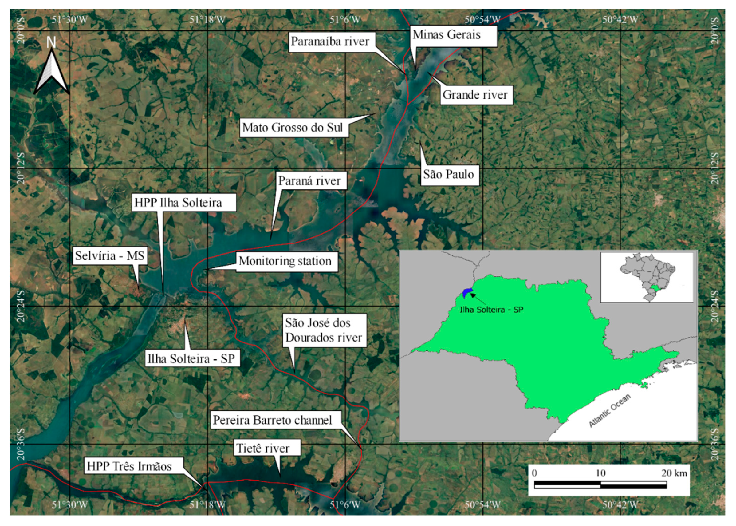
Figure 2.
Plan view representation of the bathymetry of Lake Ilha Solteira/SP.
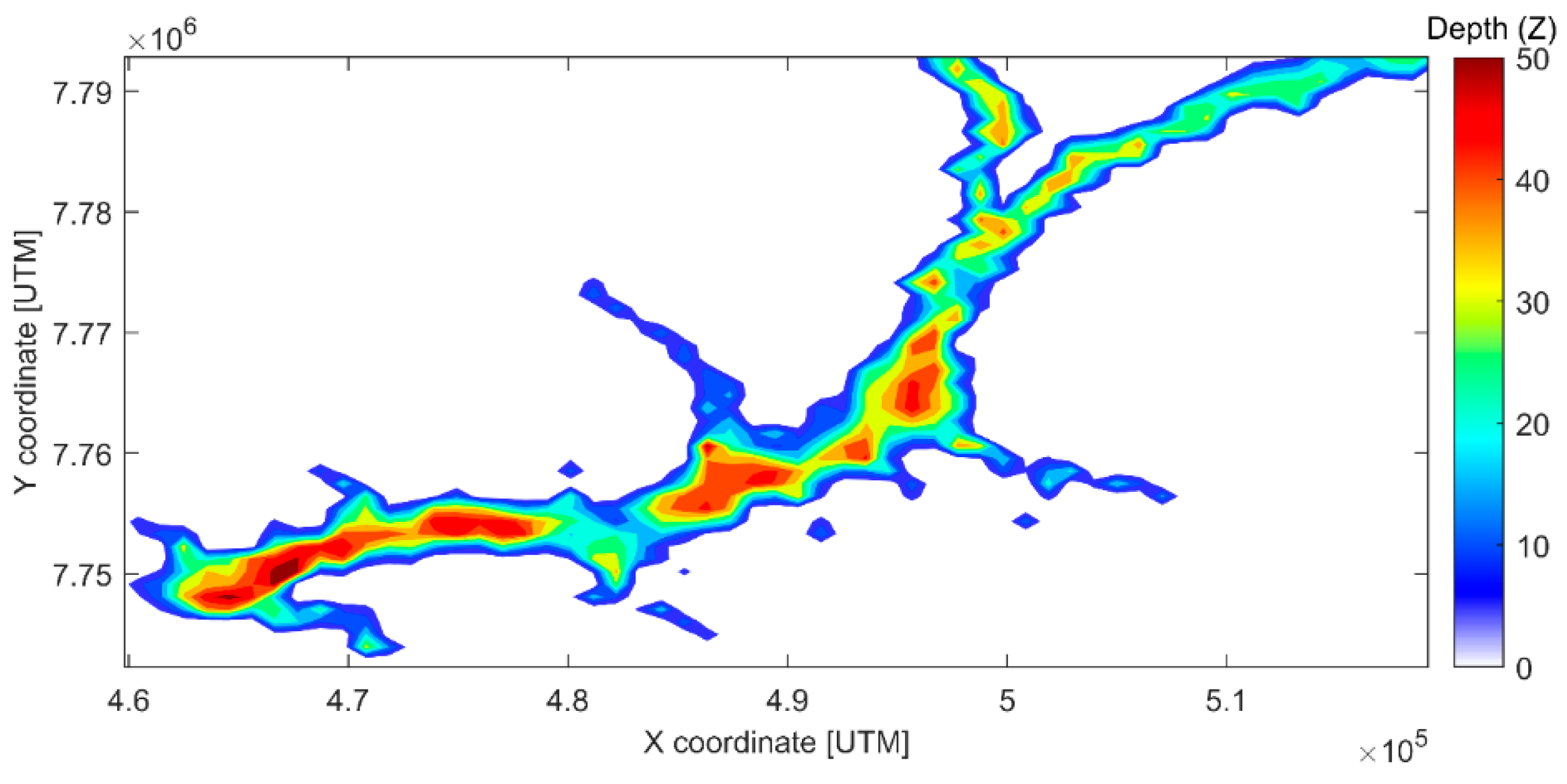
Figure 3.
Wind rose for the month of January with hourly averages of wind data (710 data points).
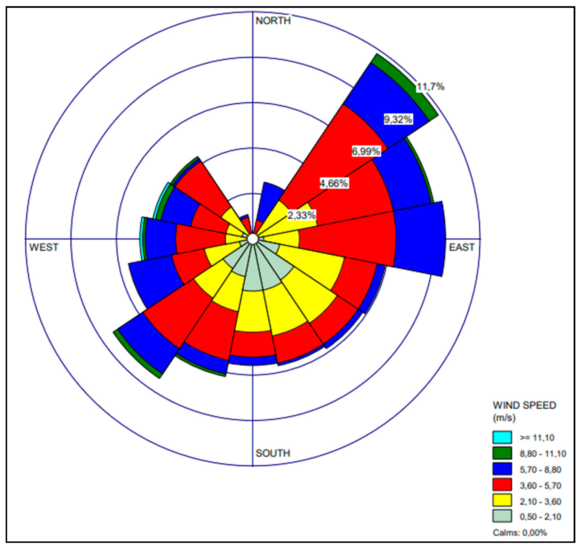
Figure 4.
Synthetic flowchart of the deterministic approach. Note: SMS (System Modeling Surface) AQUAVEO is software used to create meshes.
Figure 4.
Synthetic flowchart of the deterministic approach. Note: SMS (System Modeling Surface) AQUAVEO is software used to create meshes.
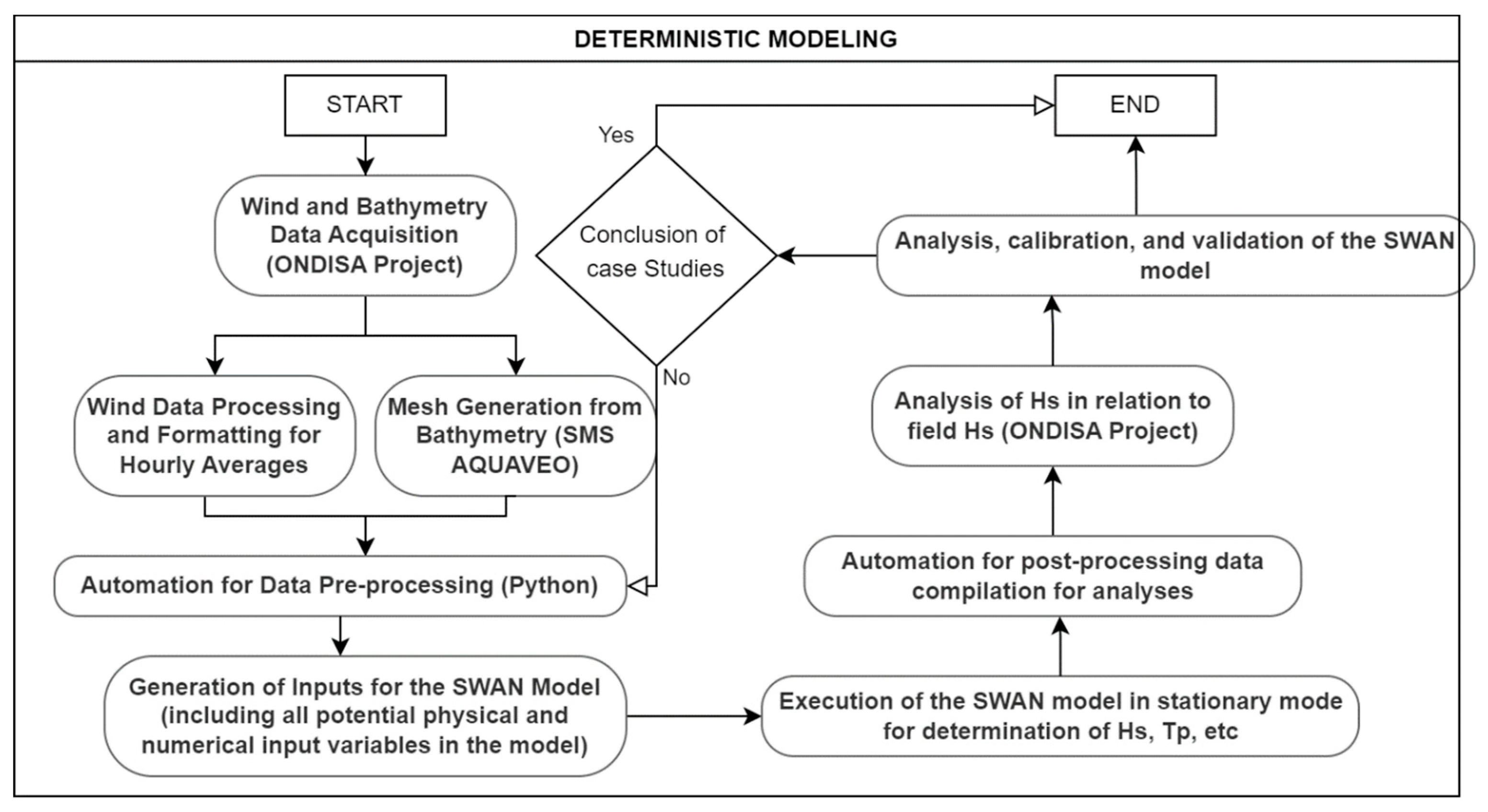
Figure 5.
Synthetic flowchart of the probabilistic approach.
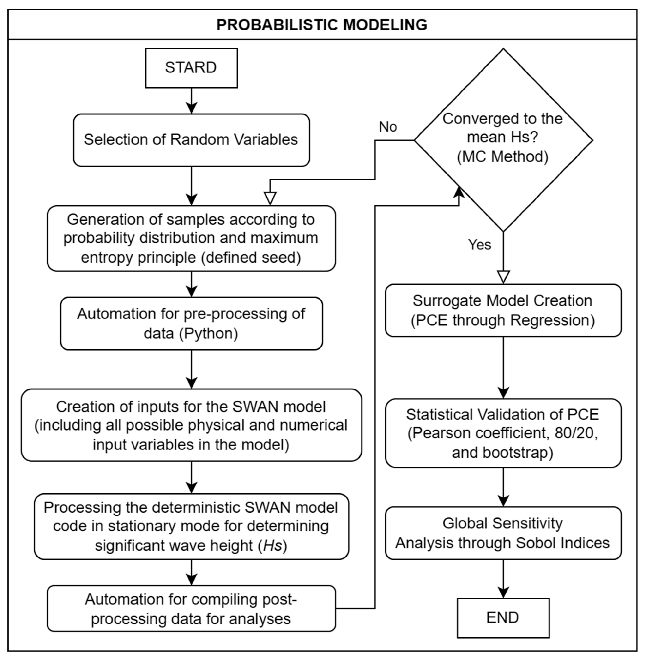
Figure 7.
Graphical representation of the probability and frequency distribution of wind speeds utilizing field data spanning from October 2010 to March 2011 (ONDISA Project database).
Figure 7.
Graphical representation of the probability and frequency distribution of wind speeds utilizing field data spanning from October 2010 to March 2011 (ONDISA Project database).
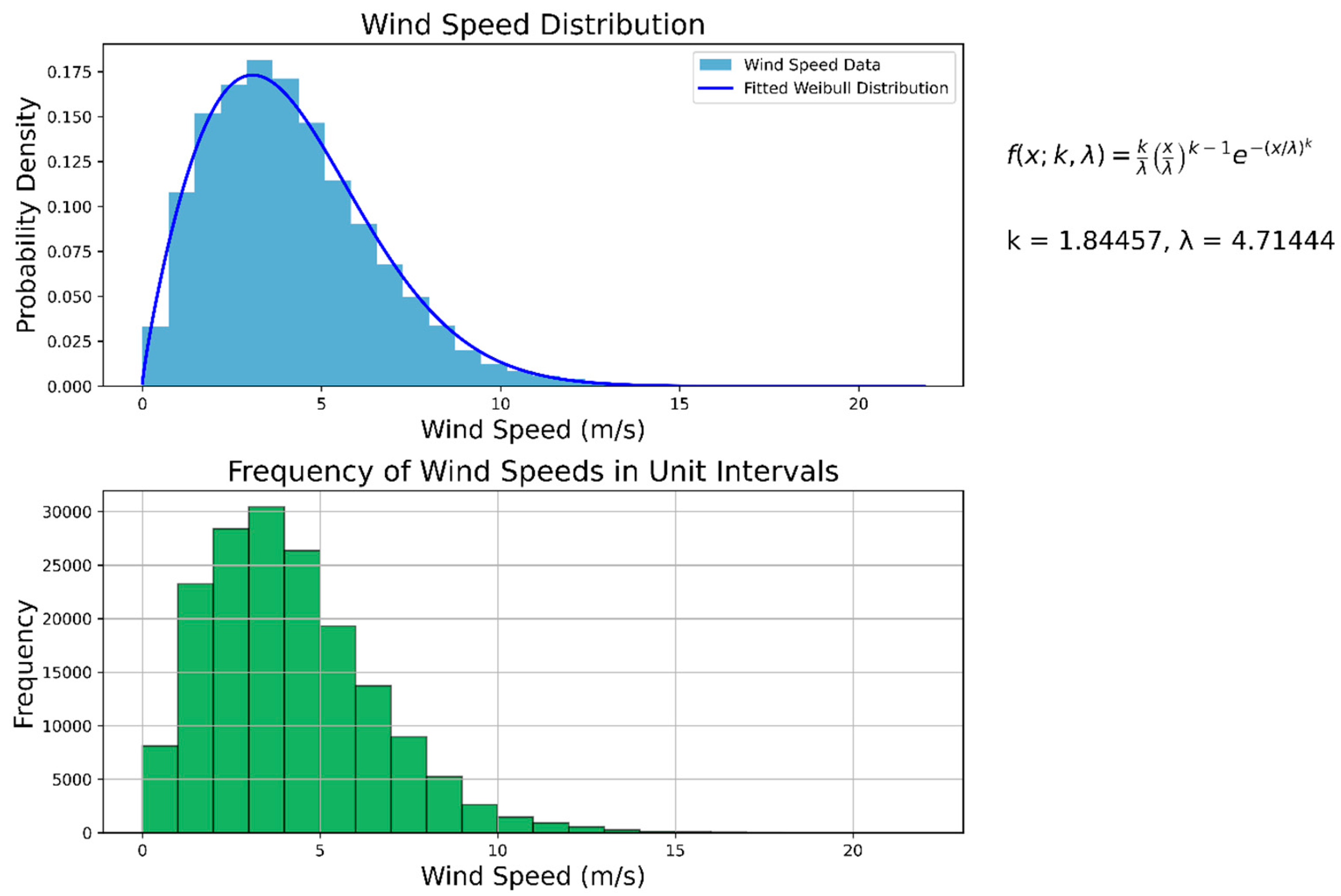
Figure 8.
Histogram of true output vs. PCE prediction.
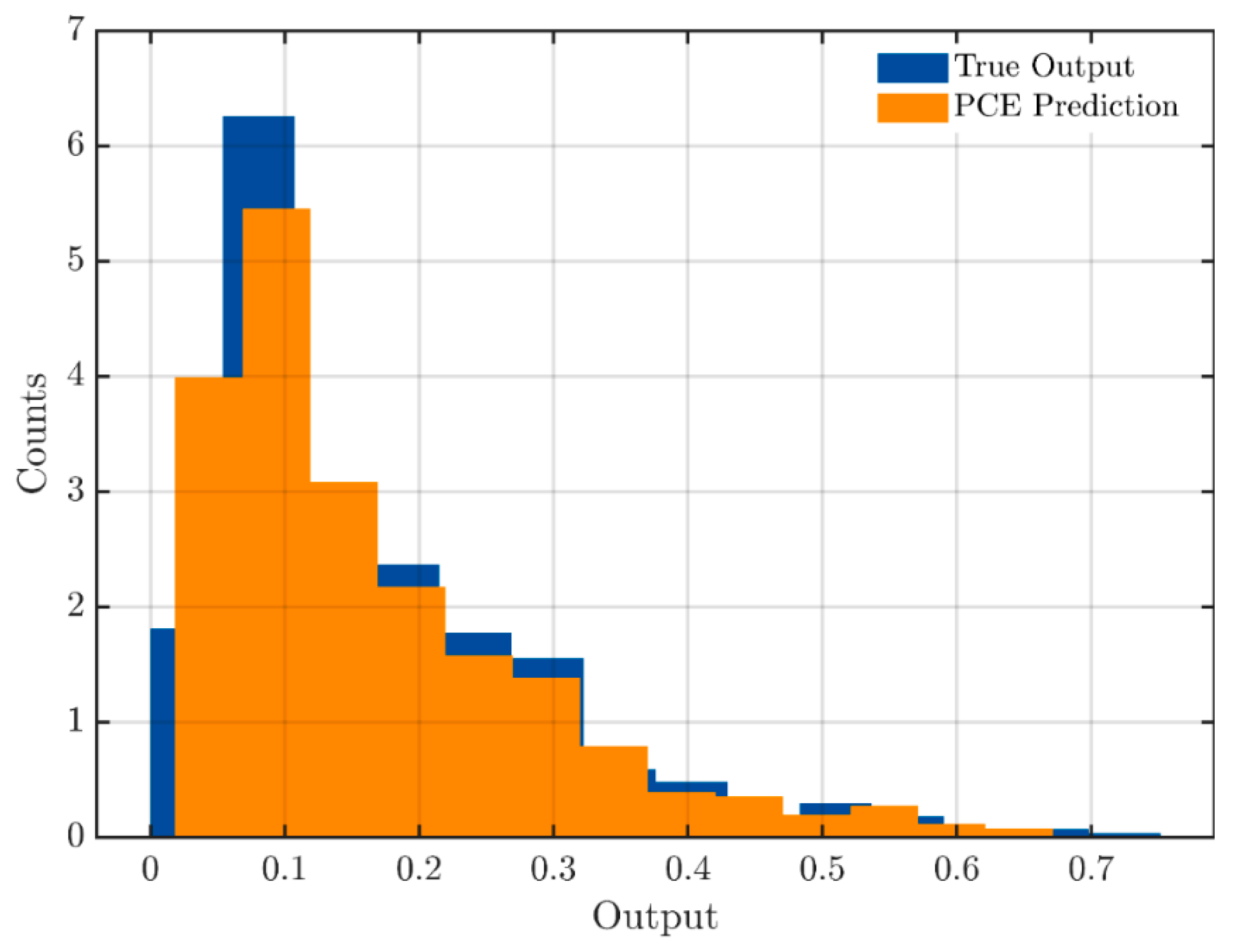
Figure 9.
First-order Sobol indices ().
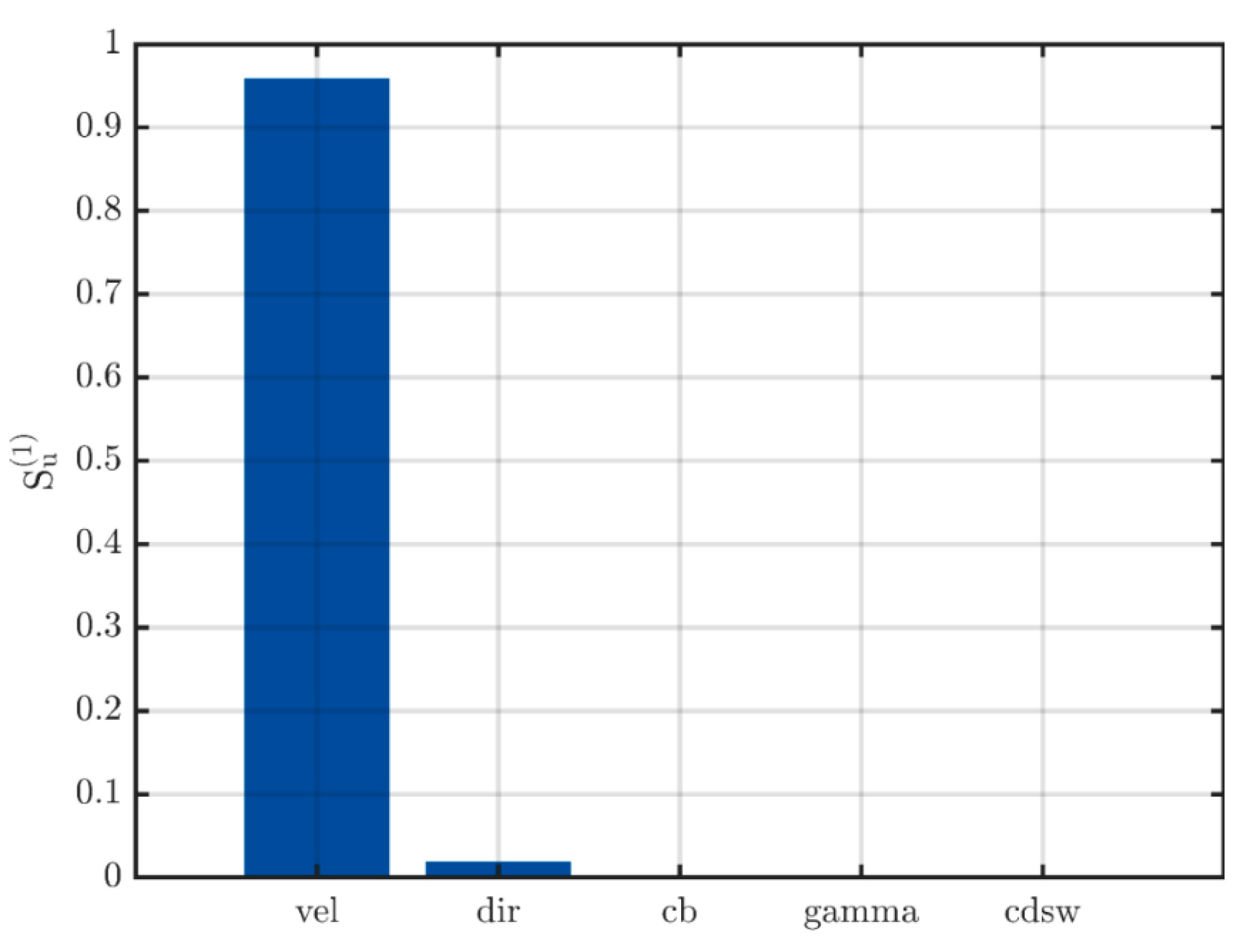
Figure 10.
Second-order Sobol indices ().
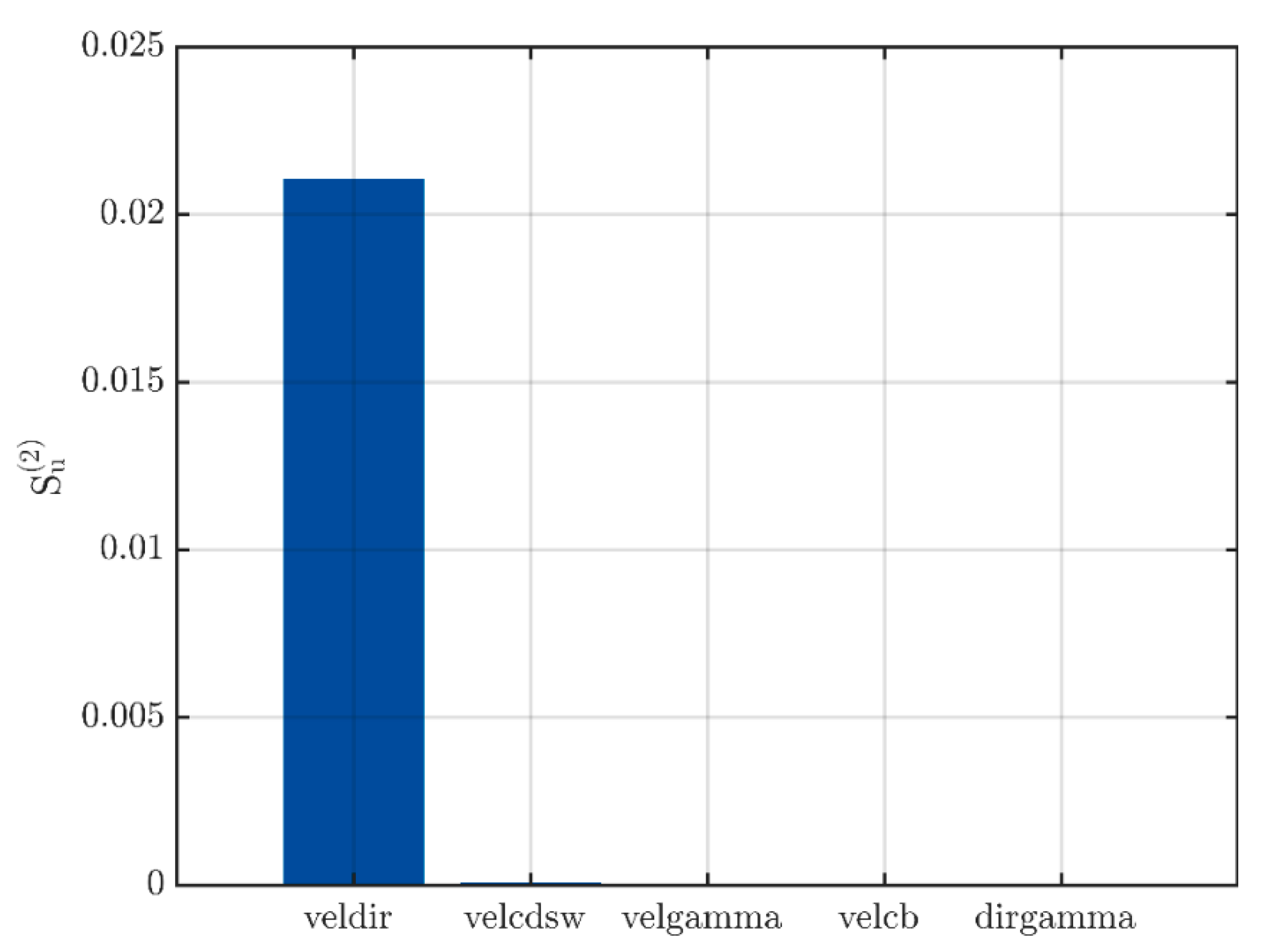
Figure 11.
Correlation and determination coefficients of the PCE.
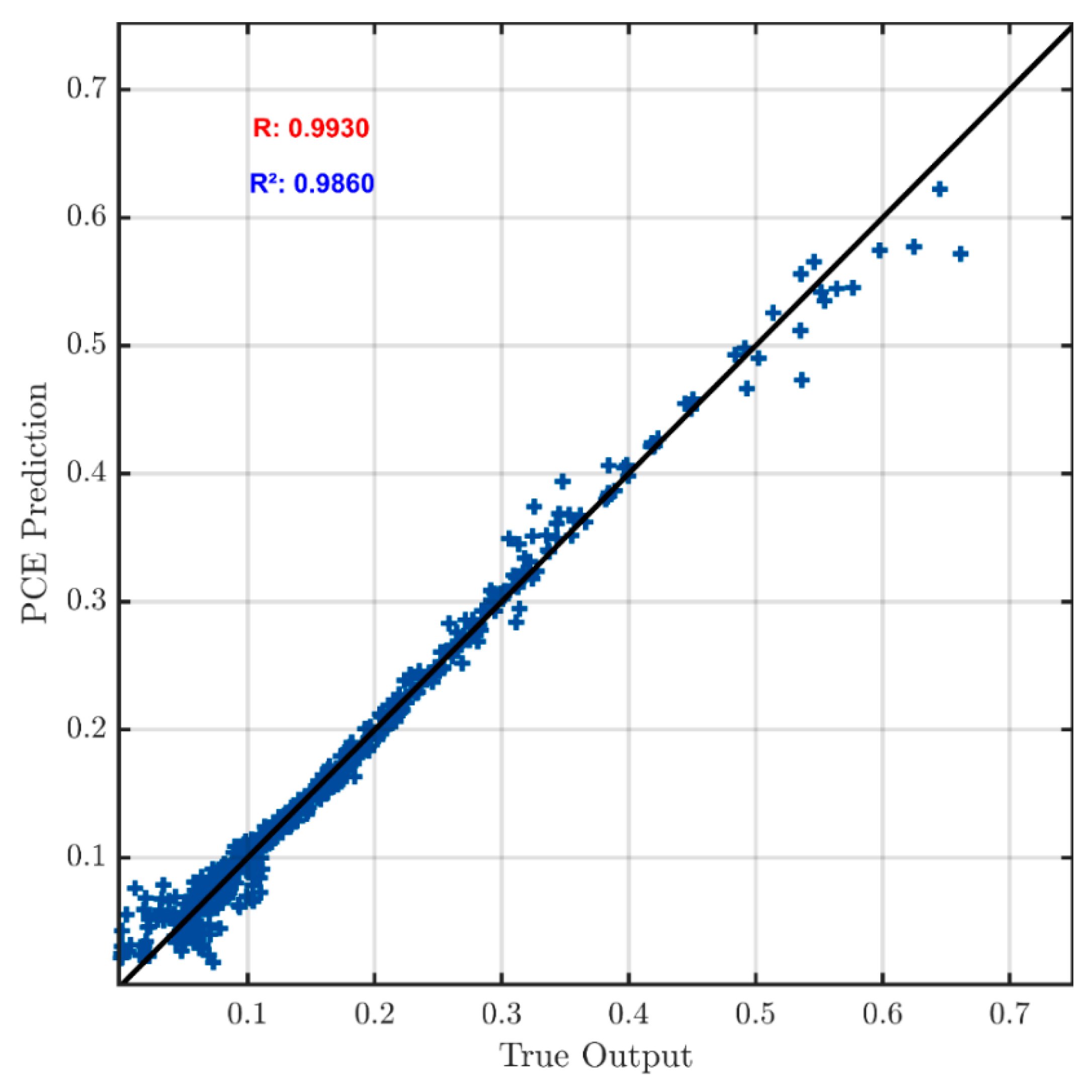
Figure 12.
Histogram of true output vs. PCE prediction with constant wind data.
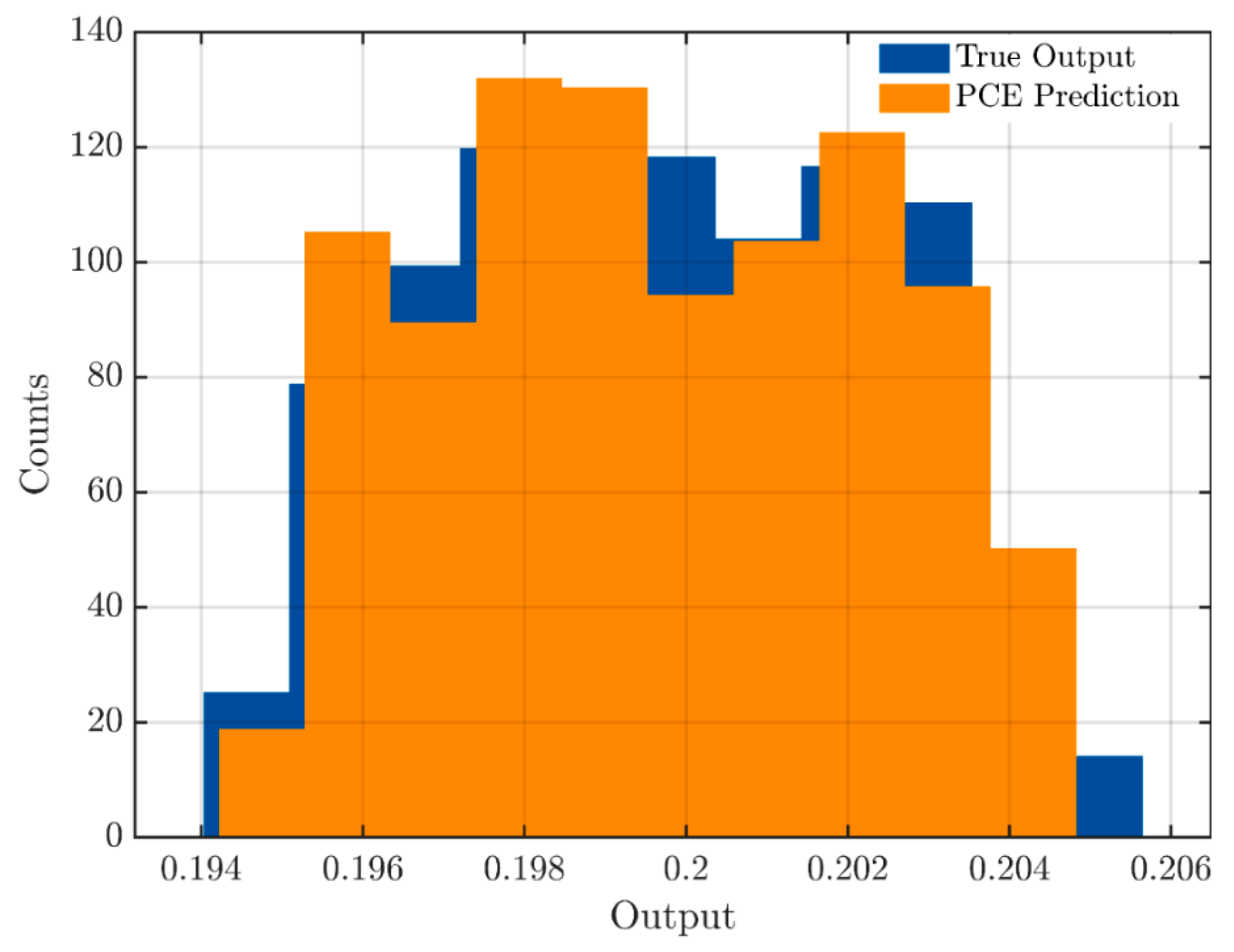
Figure 13.
First-order Sobol indices () with constant wind data.
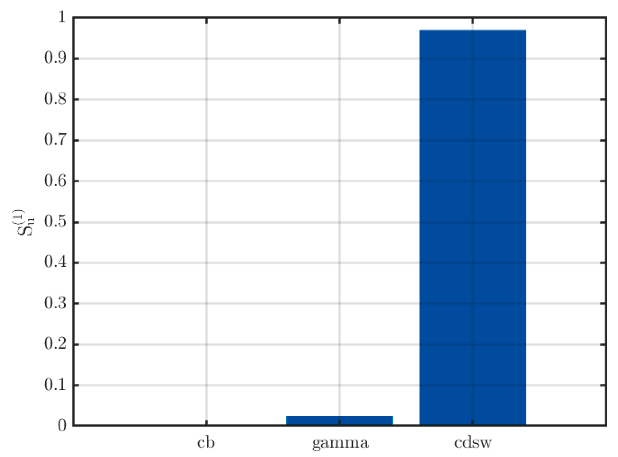
Figure 14.
Correlation and determination coefficients of the PCE with constant wind data.
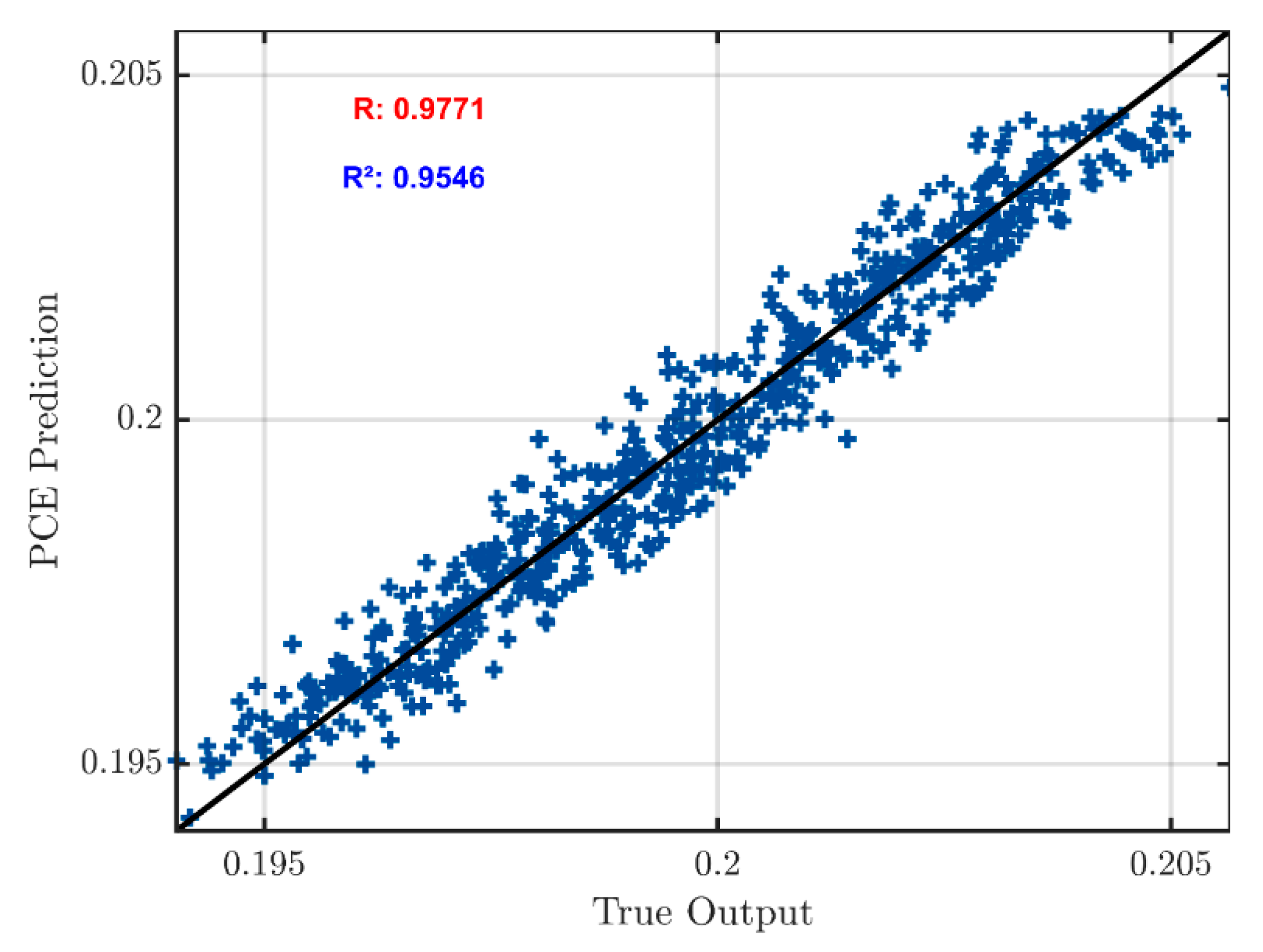
Figure 15.
Contour map of wind data in relation to .
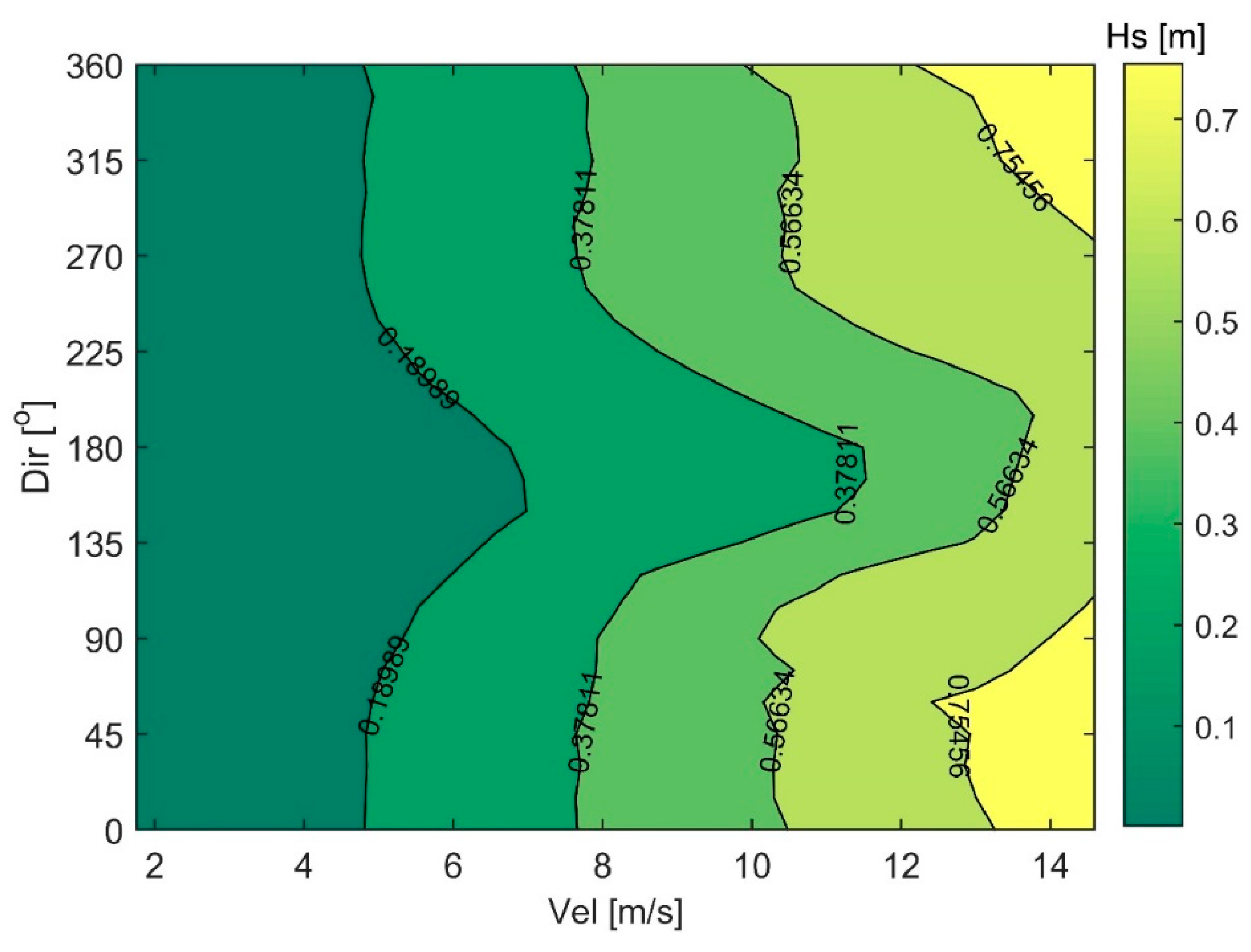
Figure 16.
Contour map of wind data in relation to the mean wave period.
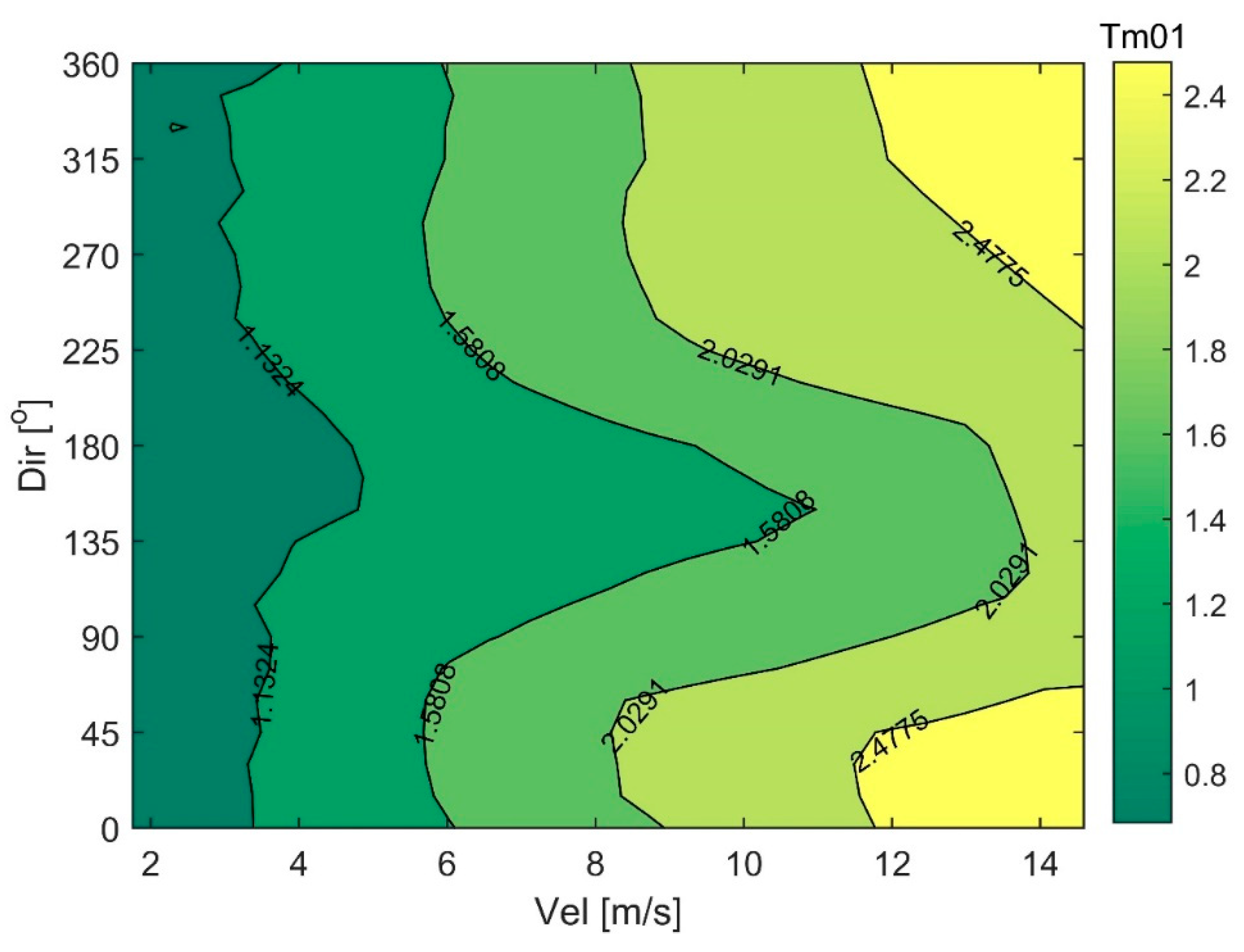
Figure 17.
Percentage distribution of mean wave propagation direction across 16 intervals for the dataset.
Figure 17.
Percentage distribution of mean wave propagation direction across 16 intervals for the dataset.
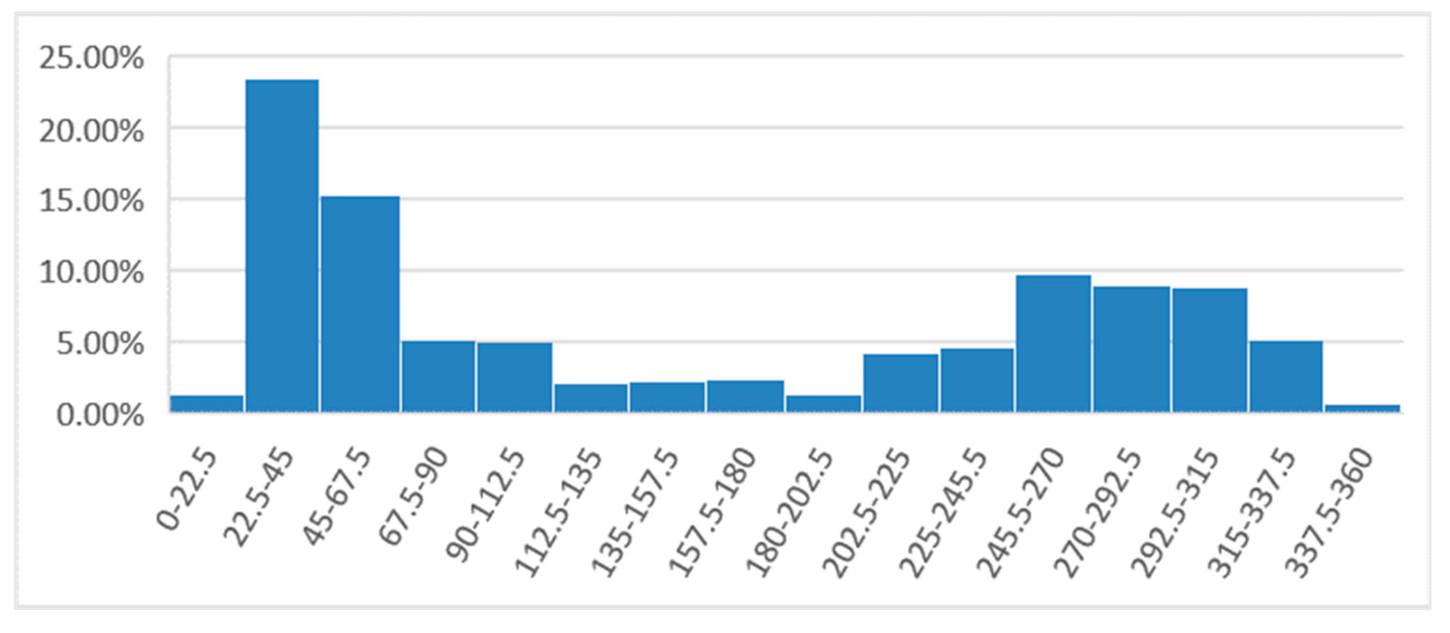
Figure 18.
Percentage distribution of peak wave propagation direction across 16 intervals for the dataset.
Figure 18.
Percentage distribution of peak wave propagation direction across 16 intervals for the dataset.
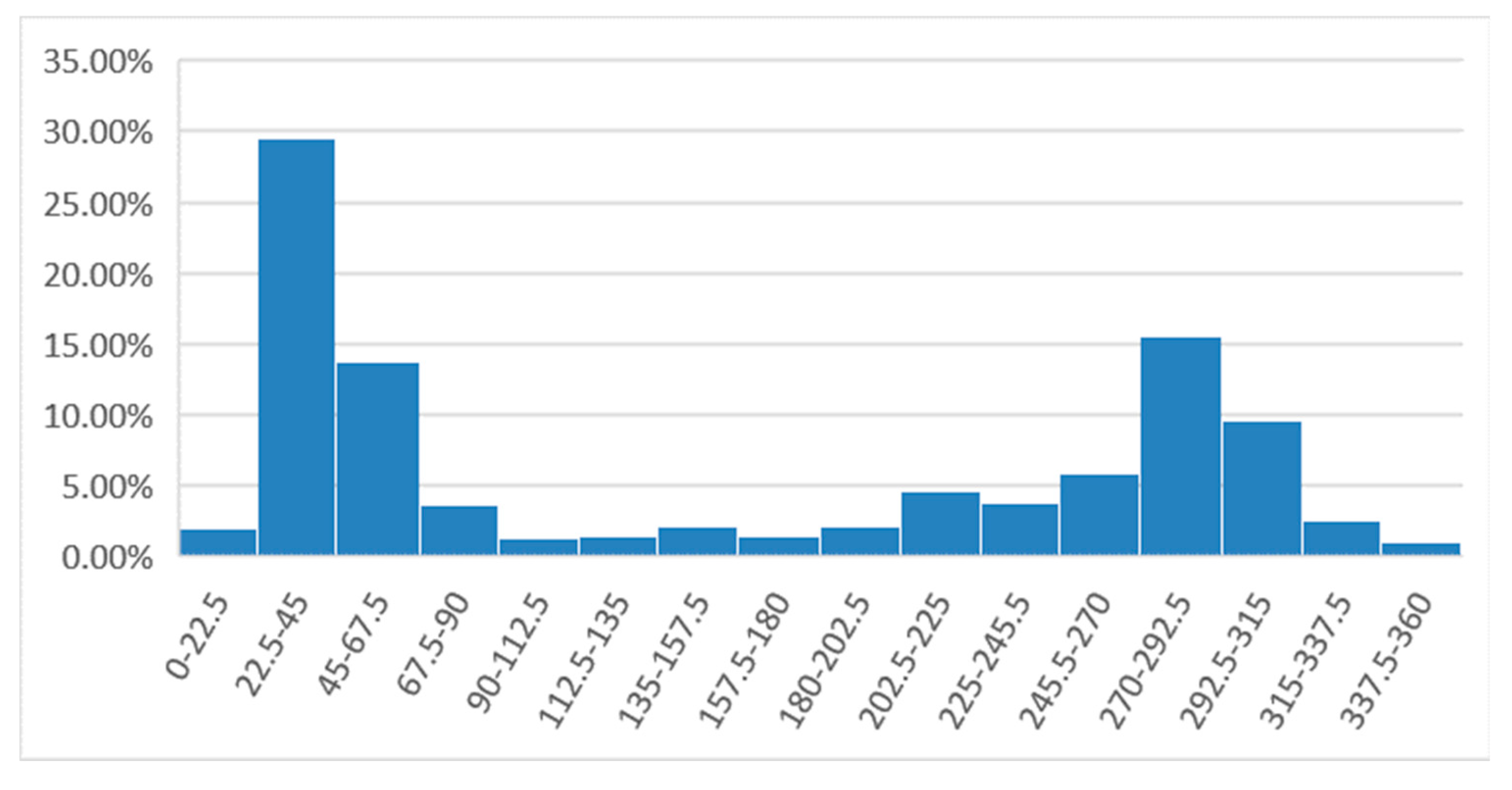
Figure 18.
Absolute mean wave propagation periods and wind speed distribution arranged for the dataset.
Figure 18.
Absolute mean wave propagation periods and wind speed distribution arranged for the dataset.
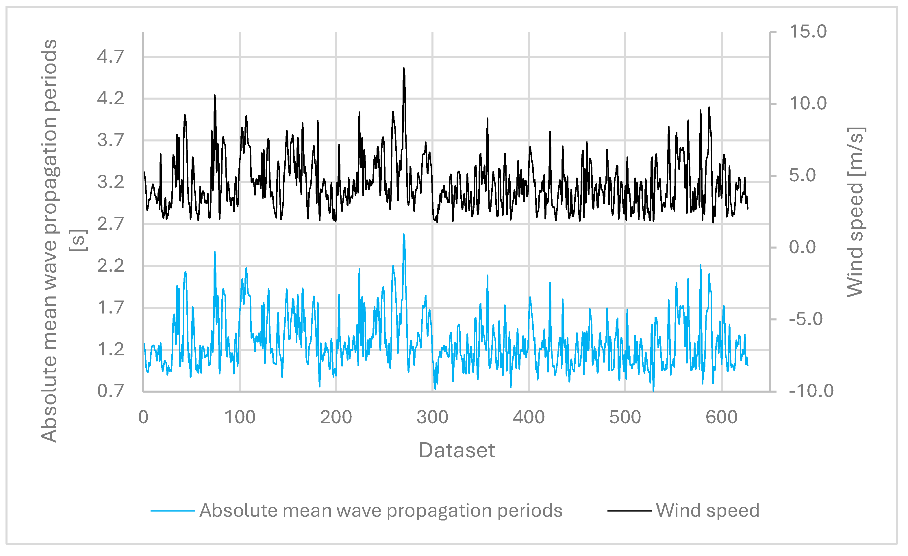
Figure 19.
Peak Period in the Variance Density Spectrum (Relative Frequency Spectrum) and Wind Speed Arranged for the Dataset.
Figure 19.
Peak Period in the Variance Density Spectrum (Relative Frequency Spectrum) and Wind Speed Arranged for the Dataset.
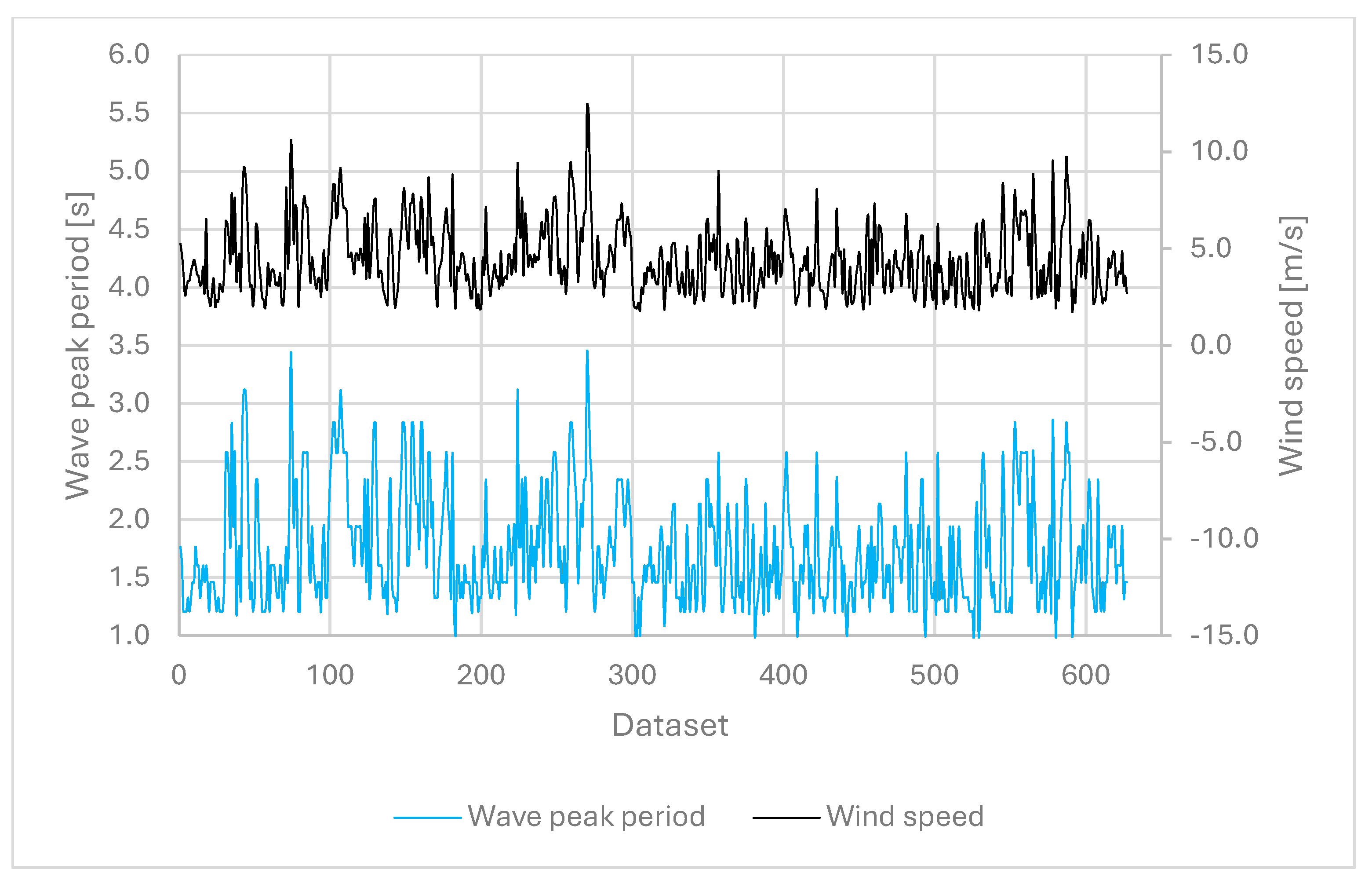

Table 1.
Characteristics of the Used Meshes.
| MESH | X COORD. [UTM] | Y COORD. [UTM] | ||
| 100 m | 458710 | 7742040 | 521 | 387 |
| 150 m | 445905 | 7741400 | 541 | 310 |
| 250 m | 459645 | 7742090 | 208 | 155 |
| 1000 m | 456680 | 7741700 | 58 | 33 |
Table 2.
Calculations for discretization of uncertainties using the GCI Method.
| Variables and parameters | Values |
| Wind speed | 5.0 m/s |
| Mesh1, Mesh2, Mesh3 | 100, 150, 250 [m] |
| No. of nodes X, Y (Mesh1) | 521, 387 |
| No. of nodes X, Y(Mesh2) | 541, 310 |
| No. of nodes X, Y(Mesh3) | 263, 174 |
| ( | 0.178, 0.177, 0.180 [m] |
| 100, 150, 250 | |
| 1.50, 1.63 (OK, | |
| 0.179 [m] | |
| 0.007 | |
| 0.006 | |
| 1.65% |
where are the representative cells (mesh Resolution); are the mesh refinement factors, with is the extrapolated value; is approximately the dimensionless relative; is the estimated value of the extrapolated relative error; and finally, is the refinement index of the lowest resolution mesh.
Table 3.
Statistical data for mesh sizes of 1000 m, 250 m, 150 m, and 100 m.
| Data | Mesh 1000 m | Mesh 250 m | Mesh 150 m | Mesh 100 m |
| (pressure sensor) | 0.0 a 0.39 m | 0.0 a 0.39 m | 0.0 a 0.39 m | 0.0 a 0.39 m |
| (SWAN) | 0.0 a 0.71 m | 0.0 a 0.70 m | 0.0 a 0.69 m | 0.0 a 0.69 m |
| 0.08 m | 0.08 m | 0.08 m | 0.08 m | |
| 0.04 m | 0.04 m | 0.04 m | 0.04 m | |
| average pressure sensor | 0.10 m | 0.10 m | 0.10 m | 0.10 m |
| average SWAN | 0.14 m | 0.14 m | 0.14 m | 0.14 m |
| 0.76 | 0.80 | 0.82 | 0.83 | |
| 0.82 | 0.81 | 0.81 | 0.80 | |
| 0.81 | 0.81 | 0.79 | 0.79 | |
| 0.67 | 0.65 | 0.64 | 0.63 |
: significant wave height; : root mean square error; : dispersion index; : concordance index; : Pearson correlation coefficient; performance index.
Table 4.
Statistical data for third-generation model formulations (GEN3) for the period of January 2011.
Table 4.
Statistical data for third-generation model formulations (GEN3) for the period of January 2011.
| Dados | GEN3 KOM | GEN3 JANS | GEN3 WESTH | |
| (pressure sensor) | 0.0 a 0.39 m | 0.0 a 0.39 m | 0.0 a 0.39 m | |
| (SWAN) | 0.0 a 0.71 m | 0.0 a 0.77 m | 0.0 a 1.59 m | |
| 0.08 m | 0.06 m | 0.20 m | ||
| 0.04 m | 0.02 m | 0.11 m | ||
| average pressure sensor | 0.10 m | 0.10 m | 0.10 m | |
| average SWAN | 0.14 m | 0.12 m | 0.21 m | |
| 0.76 | 0.64 | 2.01 | ||
| 0.82 | 0.86 | 0.58 | ||
| 0.81 | 0.79 | 0.81 | ||
| 0.67 | 0.68 | 0.47 |
: significant wave height; : root mean square error; : dispersion index; : concordance index; : Pearson correlation coefficient; performance index.
Table 5.
Statistical data for whitecapping formulations for the period of January 2011.
| Dados | WCAP KOM | WCAP JANS | WCAP LHIG | WCAP AB |
| (pressure sensor) | 0.0 a 0.39 m | 0.0 a 0.39 m | 0.0 a 0.39 m | 0.0 a 0.39 m |
| (SWAN) | 0.0 a 0.71 m | 0.0 a 0.63 m | 0.0 a 0.54 m | 0.0 a 0.59 m |
| 0.08 m | 0.06 m | 0.12 m | 0.06 m | |
| 0.04 m | 0.01 m | 0.09 m | 0.02 m | |
| average pressure sensor | 0.10 m | 0.10 m | 0.10 m | 0.10 m |
| average SWAN | 0.14 m | 0.12 m | 0.19 m | 0.12 m |
| 0.76 | 0.62 | 1.21 | 0.62 | |
| 0.82 | 0.87 | 0.67 | 0.86 | |
| 0.81 | 0.81 | 0.78 | 0.81 | |
| 0.67 | 0.70 | 0.52 | 0.70 |
: significant wave height; : root mean square error; : dispersion index; : concordance index; : Pearson correlation coefficient; performance index.
Table 6.
Supports of the considered random variables.
| VARIABLE | MINIMUM | MAXIMUM |
| Wind speed | 0.1 m/s | 22.0 m/s |
| Wind direction | 0.0° | 359.99° |
| Bottom friction coef. () | 0.029 | 0.067 |
| Depth-induced wave breaking ( | 0.3 | 0.8 |
| Whitecapping coef. | 2.124 10-5 | 2.596 10-5 |
Disclaimer/Publisher’s Note: The statements, opinions and data contained in all publications are solely those of the individual author(s) and contributor(s) and not of MDPI and/or the editor(s). MDPI and/or the editor(s) disclaim responsibility for any injury to people or property resulting from any ideas, methods, instructions or products referred to in the content. |
© 2024 by the authors. Licensee MDPI, Basel, Switzerland. This article is an open access article distributed under the terms and conditions of the Creative Commons Attribution (CC BY) license (http://creativecommons.org/licenses/by/4.0/).
Copyright: This open access article is published under a Creative Commons CC BY 4.0 license, which permit the free download, distribution, and reuse, provided that the author and preprint are cited in any reuse.


