Examination of the Spatial-Temporal Variations in Terrestrial Water Reserves and the Efficiency of Green Water Usage in China’s Three Northeastern Provinces

1. Introduction

Surface water reserves serve as an essential hydrological parameter, illustrating the aggregate impact of various water inflows and outflows in a specific region [1]. Water use efficiency (WUE) in ecosystems underscores models of carbon and water cycles, along with their interplay [2]. Most scholars have integrated the concept of the green efficiency of water resources, initially suggested by Sun Caizhi et al. [3] (2017), into their water efficiency analytical framework.

Research on water use efficiency can be classified into two types: theoretical and empirical [4]. Major techniques for the empirical quantification of water use efficiency include stochastic frontier analysis (SFA), entropy weights, and data envelopment analysis (DEA), along with derived models such as NDDF [5], SBM-Malmqist, and MinDS [6]. As research evolved, the significance of nondesired outputs came to light. This insight promoted the escalating use of SBM models in examining water use efficiency, making it the foremost measurement approach. Deng et al. (2019)[7] utilized the SBM-DEA model to assess water use efficiency across 31 Chinese provinces (municipalities and autonomous regions) using sewage discharge volume as a yardstick. Yang Gaosheng et al. (2019)[8] utilized the SE-SBM model to evaluate water use efficiency in 11 provinces (municipalities) of the Yangtze River Economic Belt, taking the human sustainable development index and total wastewater discharge as the intended and unintended outputs. Mengfei Gao et al. (2020)[9] employed the SBM-undesirable model to empirically explore the temporal and spatial progression of GWRE within the Yellow River Basin during 2003–2017. Li Jian et al. (2021)[10] applied the Super-SBM model to investigate the efficiency of green water resource utilization along with its temporal and spatial differences within the Beijing-Tianjin-Hebei urban agglomeration.

Alterations in the global gravity field are powerful tools for studying changes in terrestrial water storage [11]. The Gravity Recovery and Climate Experiment (GRACE), a joint initiative of the National Aeronautics and Space Administration (NASA) and the German Space Flight Center (DLR), generates timely gravity field data that mirror the dynamic interplay between the atmosphere, terrestrial water, oceans, and the solid Earth [12]. Wahr et al. [13] (2009) were the first to use eleven months of GRACE data to estimate water storage fluctuations in the Mississippi, Amazon River Basin, and Bay of Bengal regions. This pioneering work underscores the potential of the Earth's gravity field as a monitoring tool for regional water storage changes. GRACE has become a universally accepted tool in both global and regional research studies concerning terrestrial water storage [14]. This study utilizes GRACE data spanning from January 2003 to October 2020 to infer terrestrial water storage in the three northeastern provinces. These data are then input into the Super-SBM model to investigate the water-use efficiency in these provinces and assess the contribution of total terrestrial water resources to the utilization of water resources.

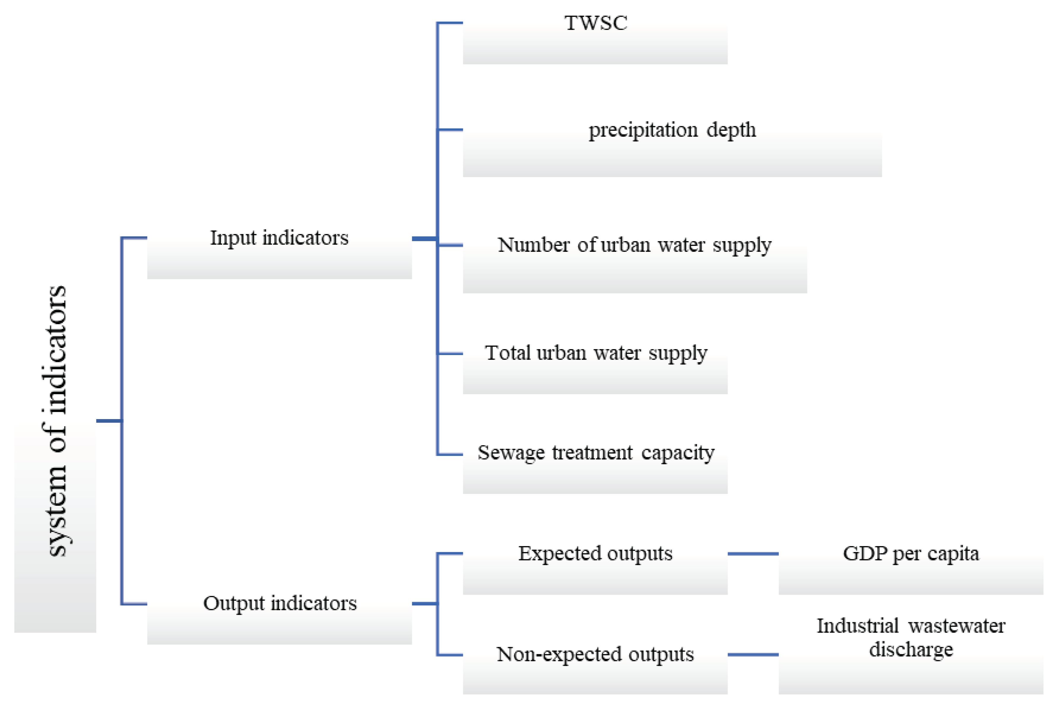
There is currently no consensus among domestic scholars regarding the establishment of a metric system for water resource utilization efficiency. The majority of scholars typically select input indicators based on factors such as capital, technology, labor, and supply, with economic output generally considered an optimal output indicator. However, water resource pollution is frequently identified as an undesirable output indicator. However, water resource pollution is frequently identified as an undesirable output indicator. He Wei[15] (2021) selected several input indicators for the DEA efficiency evaluation system of water resource utilization. These include total water supply, domestic water consumption, water-user population, employed population, and fixed asset investment within urban areas. The GDP of local municipalities is designated as the intended output indicator. In the 2022 research by Chen Yanping and colleagues[16], water resources, labor, and capital were identified as input indicators. Moreover, they considered economic output as the output indicator. In their 2010 study, Sun Caizhi et al.[17] utilized domestic and production water use, employment, and fixed asset inputs as input indicators, with GDP being the output indicator. Consequently, for this study, GDP per capita is selected as the anticipated output, while industrial wastewater discharge is viewed as the unintended output. This approach assists in creating a comprehensive water use efficiency evaluation index system. For a detailed modelling system, please refer to Figure 2.

The three eastern provinces boast abundant water resources [18,19]. However, recent population growth, misuse of water resources, and water pollution have disturbed their distribution. Studying water resource utilization has become crucial, as has efficiently monitoring spatial and temporal shifts in regional water reserves. This approach not only promotes scientific and reasonable water resource development but is also an indispensable tool for addressing water resource issues. A dearth of relevant studies on prefecture-level cities in the three eastern provinces currently prevents us from providing specific recommendations. Hence, it is crucial to conduct an in-depth study on water storage and usage within the prefecture-level cities of the three eastern provinces.

2. Data and Methods

2.1. Overview of the Study Area

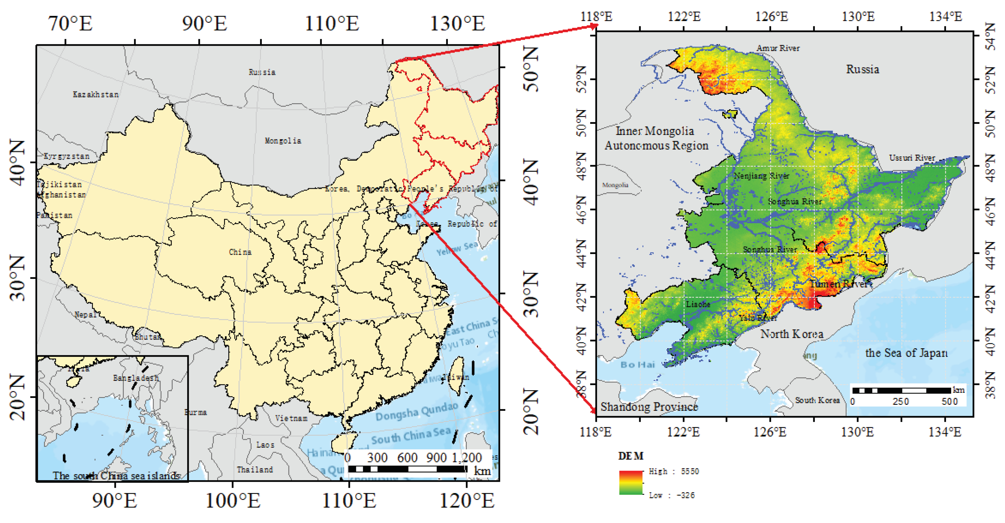
Liaoning, Jilin, and Heilongjiang constitute the three eastern provinces, encompassing a total of 36 prefectural and municipal administrative entities. This study was limited to 34 prefectural and municipal entities, as data for Yanbian Korean Autonomous Prefecture in Jilin Province and Daxinganling District in Heilongjiang Province were unavailable. Spanning an approximate area of 79.18×104 km2, the three northeastern provinces experience brief, warm summers and prolonged, chilly winters, fostering a vast water network owing to substantial snowfall and its subsequent slow melt. The region is characterized by major rivers such as Heilongjiang, Songhua, Ussuri, Mudan, Yalu and Liao, which are primarily fed by meltwater from snow and ice, precipitation, and groundwater.

This region, ideally situated amid mountains and water bodies, boasts advantageous conditions for agricultural cultivation and plays an essential role as a major grain-producing area in China. Concurrently, the trios of the eastern provinces are endowed with abundant mineral resources and represent the birthplace of heavy industry in contemporary China. The trajectory of industrial development in these three eastern provinces started at an earlier stage, and they are currently undergoing a phase of transition. Both the agriculture and industry sectors impose rigorous demands on the reserves and quality of water resources in these three eastern provinces.

Figure 1. Geographical Overview of Northeast China.

Figure 1. Geographical Overview of Northeast China.

2.2. Data Processing

2.2.1. GRACE Data

This study utilizes GRACE and GRACE-fo RL06 spherical harmonic coefficient monthly solution data furnished by the University of Texas between January 2003 and October 2020 and processes them appropriately. The specific processing steps are as follows:

(1) Execution of the spatial filtering and interpolation process

• The GRACE gravity satellite's provided spherical harmonic coefficients are employed for calculating the Earth's surface time-varying gravity field, delineated as follows:

$$\mathsf{\Delta }\delta \left(\theta ，\varphi \right)=\frac{\alpha {\rho }_{are}}{3}\sum _{i=0}^{\infty }\sum _{m=0}^l\frac{2l+1}{1+k_l}\overline{P_{lm}}(cos\theta )\times (∆C_{lm}cos(m\varphi )+∆S_{lm}sin(m\varphi ))$$

(1)

where Δδ (θ, ϕ) is the change in mass density of the Earth's surface; ρ is the Earth's mean density; α is the Earth's mean radius; $\overline{P_{lm}}(cos\theta )$ is the specified concatenated Legendre function; θ and ϕ are the Earth's core residual latitude and the Earth's core longitude, respectively; and $∆C_{lm}$ and $∆S_{lm}$_lm are the amount of change provided by GRACE.

Prior to processing the collected data from the GRACE satellite, initial preprocessing steps are essential [20]:

1) Implement a geocentric correction for its 1-degree coefficients;

2) Utilize SLR to substitute the C20 coefficients within the gravity field model;

3) Apply a blend of P3M6 decorrelation and sector filtering to the GRACE data to minimize the impact of high-frequency and correlation errors within a 300 km radius;

4) Finally, the scale factor method was used to restore signals that were diminished during the filtering and degree correction processes.

Upon completion of the aforementioned four stages of data processing, we derived TWSC gridded data specifically for the three northeastern provinces. Nevertheless, data gaps exist due to inconsistencies between the GRACE satellites and the GRACE-FO mission. Consequently, to compensate for these gaps, we utilized a restructured Chinese surface water storage dataset rooted in 2003–2020 precipitation data. This dataset originated from the China Meteorological Data Network.

The formula applied for TWSC data reformation is provided below:

$$TWS{C}_{rec}=\beta P^T$$

(2)

where $TWS{C}_{rec}$ is the TWSC data after the complementary data, P is the monthly precipitation data, β is the calibration parameter for the long-term trend term, and T is the seasonal calibration parameter.

(2) Derrending

Derrending analysis of GRACE data involves eliminating long-term trend signals from the original time series data. This procedure facilitates the erasure of incremental and decremental changes in the data's horizontal direction, thereby enabling a more effective examination of the time series data volatility variations.

2.2.2. Precipitation Data

This study sourced all required precipitation data from the China Meteorological Science Data Sharing Service Network. After referring to the data quality descriptions within the received files, we completed a preliminary review of the raw meteorological data. When data were missing, we employed the interpolation method for rectification. The scope of this study encompasses 77 meteorological stations.

2.2.3. Data on water use efficiency variables

Figure 2. Evaluation index system of water resource utilization efficiency in three northeastern provinces.

Figure 2. Evaluation index system of water resource utilization efficiency in three northeastern provinces.

2.2.4. Impact Factor Data

This research integrates pertinent indicators, emphasizing the strong correlation between water resource utilization and socioeconomic advancement in Northeast China. We selected indicators, including the economic development level, industrial structure, and socioeconomic expenditures, to examine the determining factors influencing water resource utilization across Northeast China. Acknowledging the significant impact of technological advancements and knowledge level on water resource utilization, we incorporated three additional indicators—technological progress, internationalization, and educational attainment—making a total of six indicators to thoroughly understand the factors influencing the efficiency of water resource utilization. Table 1 outlines the computation of particular indicators sourced from two datasets: the China Urban Statistical Yearbook and China Urban Construction Statistics.

2.3. Research Methodology

2.3.1. Super-SBM Modelling

Drawing upon the principle of "relative efficiency assessment", the DEA model, constructed by Charnes and Cooper, exhibits efficacy in assessing numerous decision-making units utilizing identical types of inputs and outputs; its applicability extends to analysing frontier production functions that involve complex multi-input and multioutput scenarios[21]. A DEA analytical technique—the SBM model—was proposed[22], grounded in slack variable metrics and characteristically nonradial as well as nonangular. However, this model does not exhibit a strict monotonic reduction correlated with variations in the degree of slack in both inputs and outputs[23]; moreover, it lacks effectiveness in assessing and ranking decision-making units.

$$\begin{gathered} \rho =min\frac{\frac{1}{m}\sum _{i=1}^m\overline{\frac{x_i}{x_{i0}}}}{\frac{1}{s_1+s_2}(\sum _{r=1}^{s_1}\frac{\overline{y_r}}{y_{r0}}/y_{r_0}^g+\sum _{l=1}^{s_2}\frac{\overline{b_l}}{b_{l0}})} \\ s.t.\left\{\begin{array}{c}\overline{x}\ge {\displaystyle \sum _{j=1,\ne k}^n}{\lambda }_j{x}_j\\ {\overline{y}}^g\le {\displaystyle \sum _{j=1,\ne k}^n}{\lambda }_j{y}_j^g\\ {\overline{y}}^b\ge {\displaystyle \sum _{j=1,\ne k}^n}{\lambda }_j{y}_j^b\\ \overline{x}\ge x_0,{\overline{y}}^g\le y_0^g,{\overline{y}}^b\ge {\lambda }_j{y}_0^b,{\overline{y}}^g\ge 0,\overline{{\lambda }_j}\ge 0\end{array}\right. \end{gathered}$$

(4)

where ρ is the target efficiency value; x denotes the slack variable of input indicators; ${\overline{y}}^g$ denotes the desired output; ${\overline{y}}^b$ denotes the slack variable of undesired output; $\left(\overline{x},\overline{y}\right)$ is the reference point of the decision variable; m and s are the number of input and output indicators, respectively; λ is the vector of weights; $x_j\mathrm{、}{y}_j^g \mathrm{a}\mathrm{n}\mathrm{d} y_j^b$ denote the values of the inputs, desired outputs, and undesired outputs of city j; and $x_0\mathrm{、}{y}_0^g\mathrm{、}{y}_0^b$ denote the total values of inputs, desired outputs, and nondesired outputs in the city, respectively. The urban water use efficiency is denoted by ρ. Higher values of ρ indicate greater urban water use efficiency.

2.3.2. Malmquist Exponential Modelling

Despite the optimization of the SBM model through the Super-SBM model, its analysis is restricted to a static perspective. The Malmquist exponential model, introduced by Malmquist in 1953, facilitates the dynamic analysis of productivity[24]. Despite divergent opinions in academia on the decomposition approach of the Malmquist index model, this paper utilizes the analytical technique suggested by Fare and his team. In a comparison between period t and period t+1, alterations in production efficiency can be broken down into comprehensive technical efficiency modifications (ECs) and technological progress adjustments (TCs). EC can be further subdivided into pure technical efficiency variation (PEC) and scale efficiency alteration (SEC) [25].

The following are the corresponding formulas.

$$\begin{gathered} {MI}^{t,t+1}={\left[\frac{D^t\left(x^{t+1},y^{t+1}\right)}{D^t\left(x^t,y^t\right)}\times \frac{D^{t+1}\left(x^{t+1},y^{t+1}\right)}{D^{t+1}\left(x^t,y^t\right)}\right]}^{1/2} \\ =\frac{D^{t+1}\left(x^{t+1},y^{t+1}\right)}{D^t\left(x^t,y^t\right)}{\left[\frac{D^t\left(x^t,y^t\right)}{D^{t+1}\left(x^t,y^t\right)}\times \frac{D^t\left(x^{t+1},y^{t+1}\right)}{D^{t+1}\left(x^{t+1},y^{t+1}\right)}\right]}^{1/2} \\ ={EC}^{t,t+1}\times {TC}^{t,t+1} \\ ={PEC}^{t,t+1}\times {SEC}^{t,t+1}\times {TC}^{t,t+1} \end{gathered}$$

(5)

In Eq. 8, the input indicator vectors for time periods t and t+1 are represented as $x^t$and $x^{t+1}$, respectively. Similarly, $y^t$ and $y^{t+1}$, respectively denote the output indicator vectors for these same time periods. MI denotes the variation in total factor productivity. $D^t$symbolizes the efficiency value of the DMU within period t. ${MI}^{t,t+1}>1$ suggests that the productivity of the DMU's water resources in period t+1 exceeds that of period t. ${EC}^{t,t+1}>1$implies that the DMU performance in period t is superior to that in period t+1. Finally, ${TC}^{t,t+1}>1$ indicates a shift in DMU production efficiency from period t to t+1, reflecting an enhancement in management performance.

2.3.3. Spatial Autocorrelation

This study investigated the spatial correlation of water use efficiency across three northeastern provinces between 2003 and 2020 by employing the Moran index as the analytical tool, which is defined as follows:

$$\mathrm{I}=\frac{\mathrm{n}\sum _{\mathrm{i}=1}^{\mathrm{n}}\sum _{\mathrm{j}=1}^{\mathrm{n}}{\mathrm{W}}_{\mathrm{i}\mathrm{j}}({\mathrm{X}}_{\mathrm{i}}-\overline{\mathrm{X}})({\mathrm{X}}_{\mathrm{j}}-\overline{\mathrm{X}})}{\sum _{\mathrm{i}=1}^{\mathrm{n}}\sum _{\mathrm{j}=1}^{\mathrm{n}}{\mathrm{W}}_{\mathrm{i}\mathrm{j}}\sum _{\mathrm{i}=1}^{\mathrm{n}}{({\mathrm{X}}_{\mathrm{i}}-\overline{\mathrm{X}})}^2}$$

(6)

Here, n refers to the sample size. The variables ${\mathrm{X}}_{\mathrm{i}}$and ${\mathrm{X}}_{\mathrm{j}}$ represent the mobile populations of the ith and jth cities, respectively. The average mobile population across all cities is denoted by $\overline{\mathrm{X}}$. Additionally, ${\mathrm{W}}_{\mathrm{i}\mathrm{j}}$ is an element of the spatial weight matrix intended to assist in the positioning of mobile population data for comparative geospatial analysis in the geographic area being studied.

The previous formula represents the global spatial autocorrelation analysis. For an observation at a given site, we calculate the Moran's I statistic as follows:

$${\mathrm{I}}_{\mathrm{i}}\left(\mathrm{d}\right)={\mathrm{Z}}_{\mathrm{i}}\sum {\mathrm{W}}_{\mathrm{i}\mathrm{j}}{\mathrm{Z}}_{\mathrm{j}}$$

(7)

where ${\mathrm{Z}}_{\mathrm{i}}$ and ${\mathrm{Z}}_{\mathrm{j}}$ are normalized patterns of observations.

(i) Tobit regression model

The Tobit model is a regression model in which the dependent variable for regression analysis is constrained, as the values derived from the Super-SBM model are invariably positive. The Tobit model typically applies when various conditions constrain the type of the dependent variable[26]. The prerequisites for implementing the Tobit model includes: (1) the two segments of the explanatory variables being distinct and (2) the random variable aligning with the joint normal distribution during the model assumptions, exemplified by the following formula:

$$\begin{gathered} y^{*}=\beta X_i+\mu i \\ {y}_i=\left\{\begin{array}{c}{y}_i^{*} if{y}_i^{*}>0 \\ 0 if{y}_i^{*}<0\end{array}\right. \end{gathered}$$

(8)

The latent variable is represented as $y^{\mathrm{*}}$, while the finite dependent variable is given by $y_i$. $X_i$ is utilized as the explanatory variable, with the correlation coefficient denoted by β. The random error is denoted as μ, and the ith decision unit is denoted as i.

Based on equation (8), the regression assumptions are as follows:

$$y_{i,t}={\beta }_0+{\beta }_1{GDP}_{i,t}+{\beta }_2{CY}_{i,t}+{\beta }_3{OPEN}_{i,t}+{\beta }_4{E}_{i,t}+{\beta }_5{G}_{i,t}+{\epsilon }_{i,t}$$

(9)

In this study, ${\mathrm{G}\mathrm{D}\mathrm{P}}_{\mathrm{i},\mathrm{t}}$ refers to the growth rate of gross domestic product, and ${\mathrm{C}\mathrm{Y}}_{\mathrm{i},\mathrm{t}}$represents the industrial structure. ${\mathrm{O}\mathrm{P}\mathrm{E}\mathrm{N}}_{\mathrm{i},\mathrm{t}}$ signifies the level of openness to foreign trade, depicted by the ratio of export volume to GDP. ${\mathrm{E}}_{\mathrm{i},\mathrm{t}}$ stands for education level, represented by the proportion of enrolled students at all levels in the total population at year end. ${\mathrm{G}}_{\mathrm{i},\mathrm{t}}$ describes the various social economic expenditures, demonstrated by the share of general public budget expenditures in GDP. ${\mathsf{\epsilon }}_{\mathrm{i},\mathrm{t}}$ is a disturbance term.

3. Spatial and Temporal Analysis of Terrestrial Water Reserves

Figure 3 illustrates the spatial distribution of terrestrial water resources across the three eastern provinces, indicating that the northern regions have greater water resources than do the southern areas. The maximum value of the terrestrial water storage capacity (TWSC), 8.32, is located near the Qiqihar-Heihe border in Heilongjiang Province. This high value denotes a stable and surplus water storage capacity in this region over an extended period. The minimum TWSC value of -4.64 was noted in Liaoyang city, Liaoning Province, indicating a prolonged deficit in surface water storage in this region. Geographically, the surface water storage in Jilin and Liaoning Provinces is significantly lower than that in Heilongjiang Province.

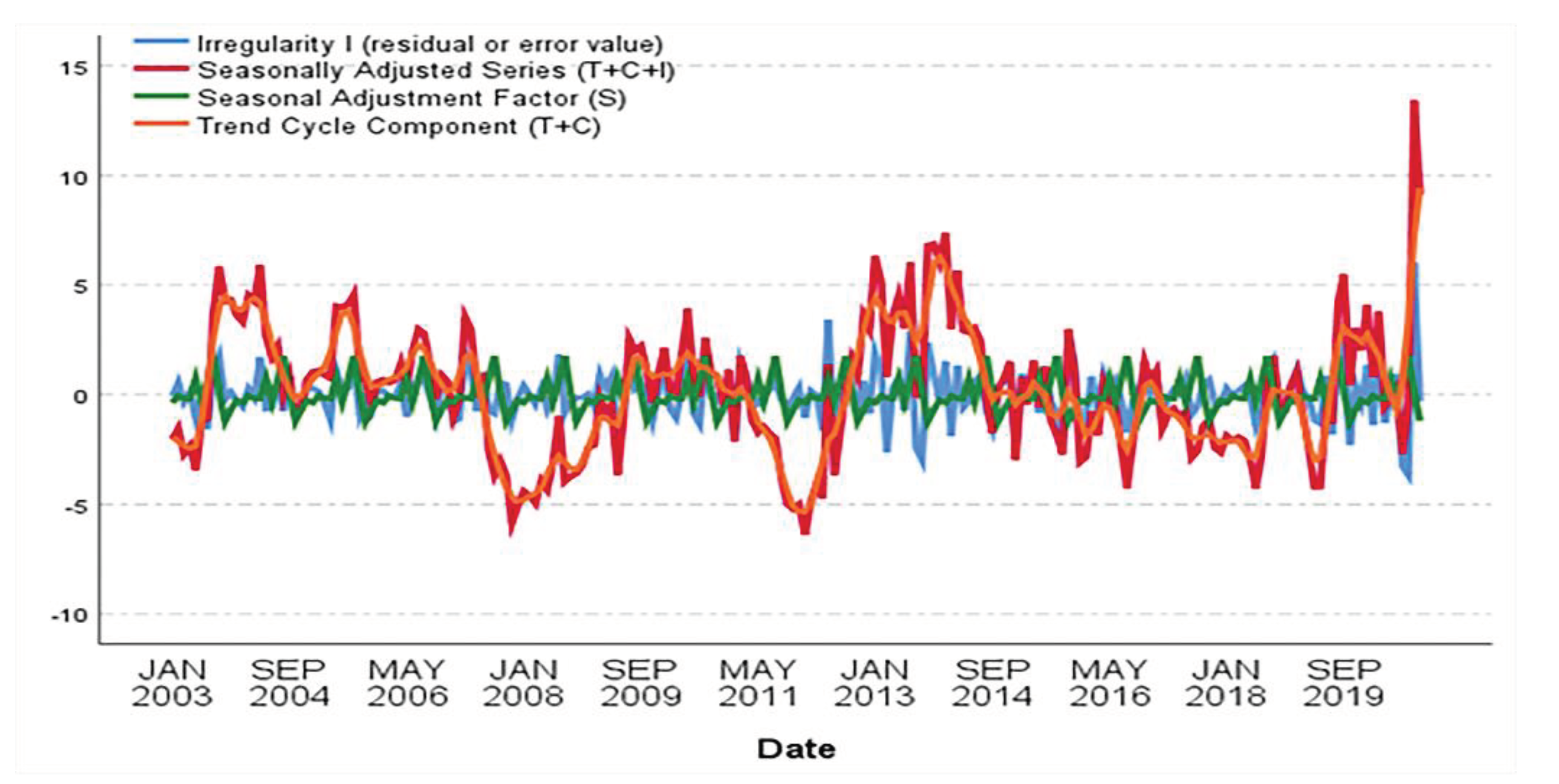
Time-dimensional observations (depicted in Figure 4) reveal the abundance of water resources in the three eastern provinces during spring and summer, with contrasting scarcity in autumn and winter. This pattern aligns with the geographical features associated with Northeast China's high summer rainfall, northern latitudinal position, cooler temperatures, and springtime snow melt. By analysing the seasonality of the TWSA time series [27] (displayed in Figure 5), our findings suggest insignificant seasonal variation in the terrestrial water resources of the three eastern provinces. However, the cyclical fluctuation in its trend is pronounced and mirrors that of the TWSA time series.

Figure 3. Spatial distribution of the mean terrestrial water storage in the three northeastern provinces from 2003 to October 2020.

Figure 3. Spatial distribution of the mean terrestrial water storage in the three northeastern provinces from 2003 to October 2020.

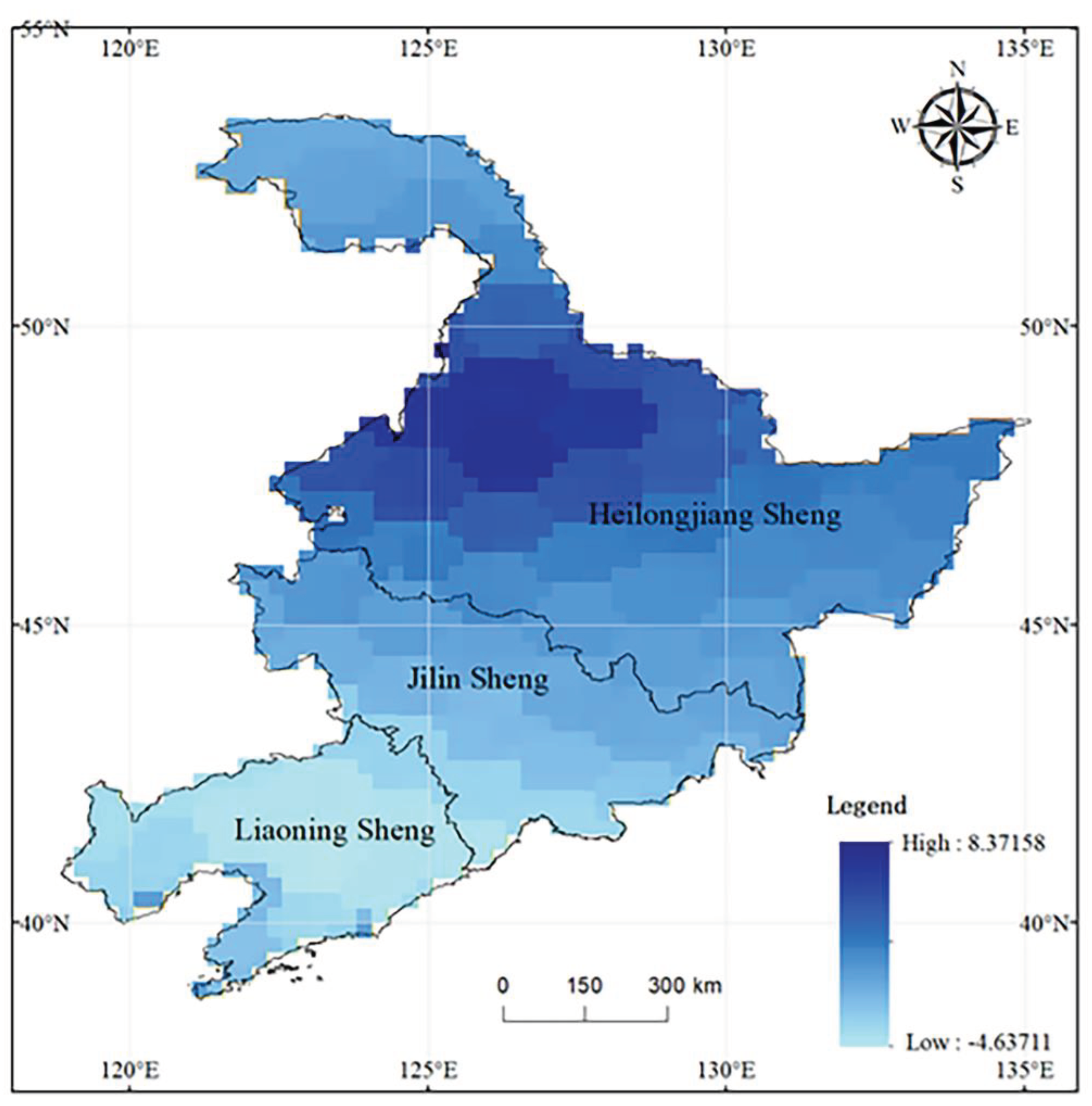
Figure 4. Time series of terrestrial water resource reserves in the three northeastern provinces from January 2003 to October 2020.

Figure 4. Time series of terrestrial water resource reserves in the three northeastern provinces from January 2003 to October 2020.

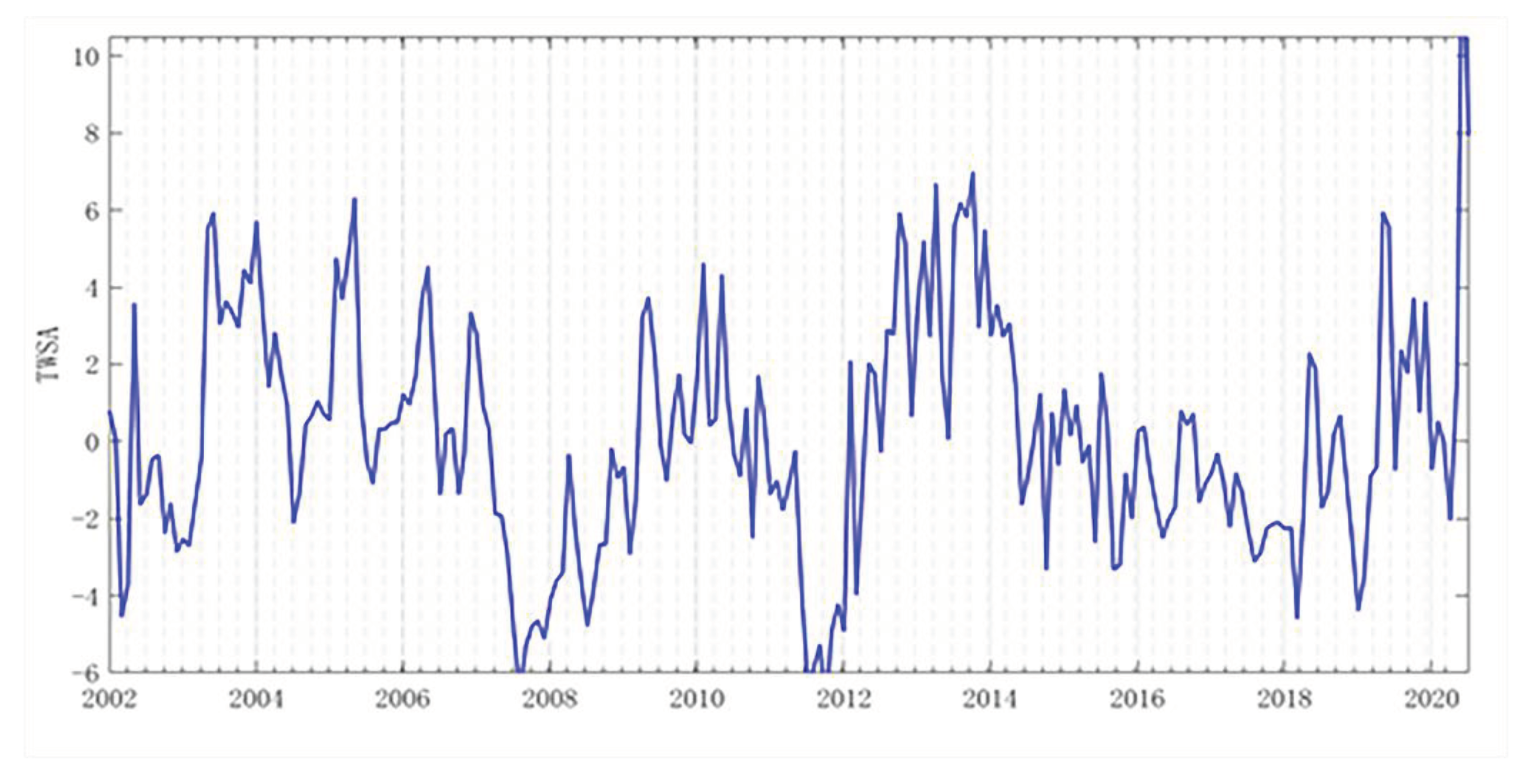
Figure 5. Seasonal decomposition of the time series of terrestrial water resources in the three northeastern provinces from January 2003 to October 2020.

Figure 5. Seasonal decomposition of the time series of terrestrial water resources in the three northeastern provinces from January 2003 to October 2020.

4. Water Use Efficiency Analysis

4.1. Static Water Use Efficiency Analysis

We applied a nondirected Super-SBM-based measurement to analyse the water use efficiency of 34 prefecture-level cities across three eastern provinces between 2003 and 2020 by calculating annual figures for each region. As depicted in Table 2, out of 612 static efficiency values, 248 values greater than or equal to 1 constituted 40.52% of the sample. These valid measurements provide valuable data for subsequent research.

Through a rigorous study, we obtained a robust understanding of static water use efficiency across the three eastern provinces and calculated the yearly mean static water efficiency for 34 prefecture-level cities [28,29] (refer to Table 3). Among the assessed cities, Panjin exhibited the maximum static water utilization efficiency, in stark contrast to Qiqihar, which demonstrated the lowest efficiency. We established 1 and 0.6 as benchmarks for demarcating high, medium, and low efficiency levels. Broadly, the three northeastern provinces demonstrate commendable water use efficiency, with 91.18% of the cities showcasing either medium or high efficiency levels. Nonetheless, certain areas, including Jilin, Harbin, and Qiqihar, display water utilization efficiencies lower than 0.6, indicating a pressing need for improvements in their water utilization efficiencies.

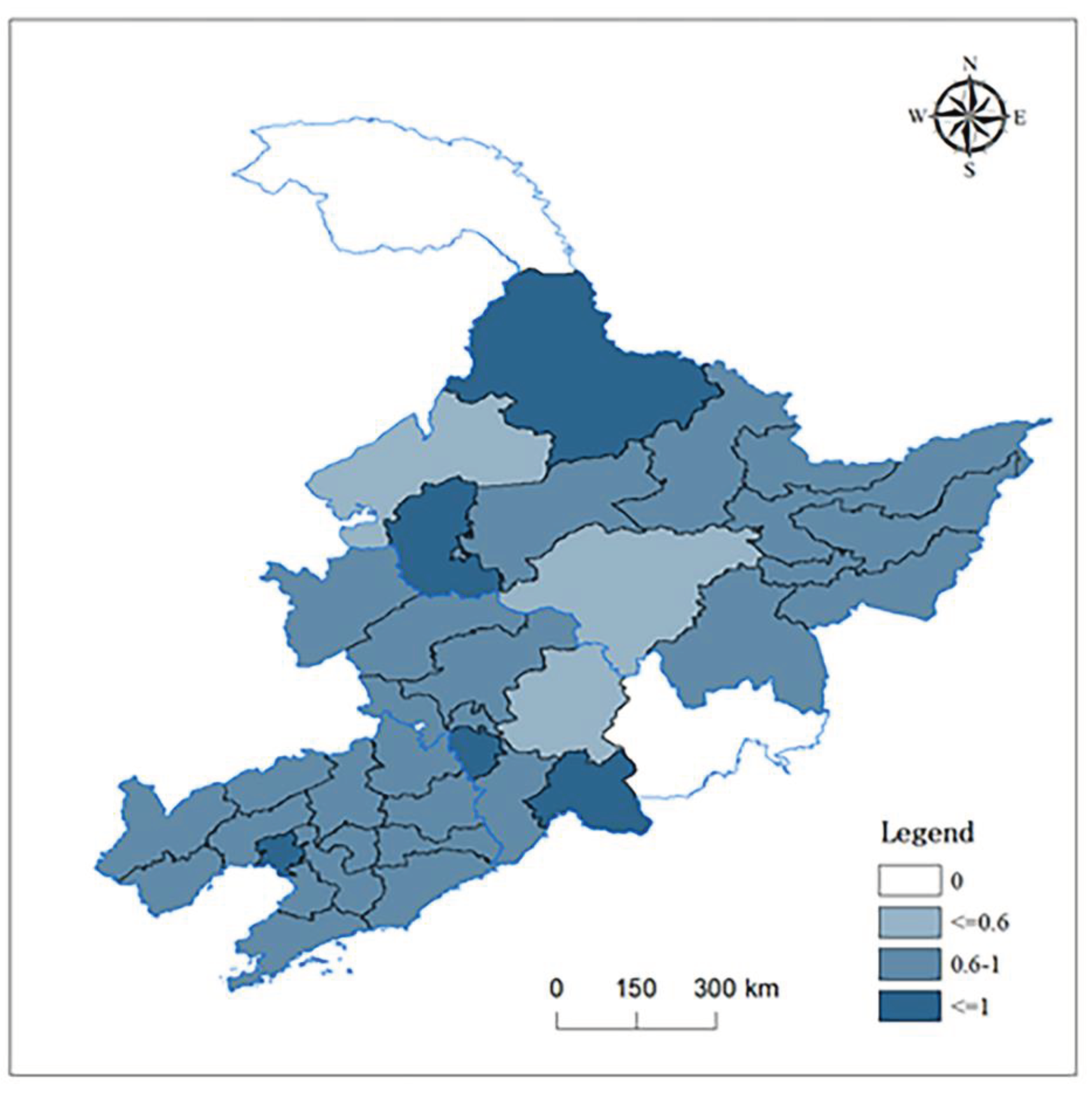
According to the spatial distribution (Figure 6), cities utilizing water resources efficiently are scattered geographically, potentially hindering the maximum exploitation of economies of scale. Regions at interprovincial borders, such as Daqing, Liaoyuan, and Baishan, are often home to cities with comparatively high water use efficiency. The northern region exhibits a diverse blend of areas with both high and low water use efficiency, displaying more pronounced regional disparities compared to its southern counterpart. Nonetheless, the southern region demonstrates a relative balance in overall water use efficiency, with a mean efficiency ranging from 0.6 to 1.

Table 2. Number of 34 prefecture-level cities in the three northeastern provinces with a static efficiency value of water resource utilization efficiency ≥ 1 from 2003 to 2020.

Year (years)	2003	2004	2005	2006	2007	2008	2009	2010	2011	Total
Number of valid values (in pieces)	16	16	11	10	3	6	22	13	12	248
Year (years)	2012	2013	2014	2015	2016	2017	2018	2019	2020
Number of valid values (in pieces)	13	12	14	18	17	14	18	17	16

Table 2. Number of 34 prefecture-level cities in the three northeastern provinces with a static efficiency value of water resource utilization efficiency ≥ 1 from 2003 to 2020.

Year (years)	2003	2004	2005	2006	2007	2008	2009	2010	2011	Total
Number of valid values (in pieces)	16	16	11	10	3	6	22	13	12	248
Year (years)	2012	2013	2014	2015	2016	2017	2018	2019	2020
Number of valid values (in pieces)	13	12	14	18	17	14	18	17	16

Table 3. The average value of the water resource utilization rate in 34 prefecture-level cities in the three northeastern provinces.

Region	Mean	Ranking	Region	Mean	Ranking
Panjin	1.13	1	Fuxin	0.77	18
Heihe	1.11	2	Hegang	0.76	19
Daqing	1.09	3	Suihua	0.74	20
Liaoyuan	1.02	4	Jiamusi	0.72	21
Baishan	1.02	5	Jixi	0.71	22
Yichun	0.98	6	FUshun	0.70	23
Baicheng	0.95	7	Shenyang	0.69	24
Songyuan	0.92	8	Dandong	0.69	25
Chaoyang	0.90	9	Anshan	0.69	26
Tonghua	0.85	10	Yingkou	0.68	27
Dalian	0.83	11	Jinzhou	0.66	28
Tieling	0.83	12	Huludao	0.63	29
Benxi	0.82	13	Mudanjiang	0.63	30
Shuangyashan	0.82	14	Changchun	0.61	31
Siping	0.81	15	Jilin	0.54	32
Qitaihe	0.79	16	Harbin	0.52	33
Liaoyang	0.77	17	Qiqihar	0.44	34

Table 3. The average value of the water resource utilization rate in 34 prefecture-level cities in the three northeastern provinces.

Region	Mean	Ranking	Region	Mean	Ranking
Panjin	1.13	1	Fuxin	0.77	18
Heihe	1.11	2	Hegang	0.76	19
Daqing	1.09	3	Suihua	0.74	20
Liaoyuan	1.02	4	Jiamusi	0.72	21
Baishan	1.02	5	Jixi	0.71	22
Yichun	0.98	6	FUshun	0.70	23
Baicheng	0.95	7	Shenyang	0.69	24
Songyuan	0.92	8	Dandong	0.69	25
Chaoyang	0.90	9	Anshan	0.69	26
Tonghua	0.85	10	Yingkou	0.68	27
Dalian	0.83	11	Jinzhou	0.66	28
Tieling	0.83	12	Huludao	0.63	29
Benxi	0.82	13	Mudanjiang	0.63	30
Shuangyashan	0.82	14	Changchun	0.61	31
Siping	0.81	15	Jilin	0.54	32
Qitaihe	0.79	16	Harbin	0.52	33
Liaoyang	0.77	17	Qiqihar	0.44	34

Figure 6. Spatial distribution map of the mean value of water resource utilization in 34 prefecture-level cities in the three northeastern provinces from 2003 to 2020.

Figure 6. Spatial distribution map of the mean value of water resource utilization in 34 prefecture-level cities in the three northeastern provinces from 2003 to 2020.

4.2. Dynamic Water Use Efficiency Analysis

The Super-SBM model fails to represent temporal variations in water use efficiency [30]. We employed DEAP 2.1 software to assess the dynamic water use efficiency in the three eastern provinces from 2003 to 2020, leveraging the chosen evaluation index system (refer to Table 4 for more details). Of the 578 calculated dynamic water efficiency scores, 333 exceeded 1, constituting 57.61% of the total sample size. This suggests that nearly half of the cities in the three eastern provinces have enhanced their water use efficiency compared to the preceding year, suggesting a steady improvement in the water utilization capacity of these prefecture-level cities.

We arrange and deconstruct the time series pertaining to the efficiency of dynamic water resources[31], as illustrated in Figure 7. The following content presents the results of this analysis:

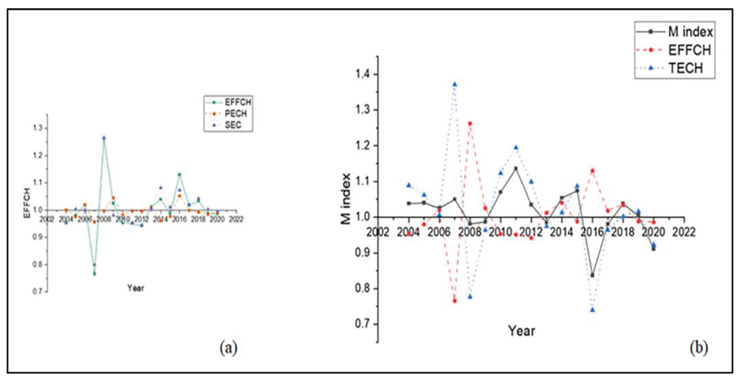
(1) In general, the average total factor productivity in the three northeastern provinces is 1.012, with an annual growth rate of 1.2%. The consistency between dynamic water resource utilization efficiency and the technological progress efficiency index is strong. To improve the water resource utilization efficiency in northeastern cities, it is necessary to introduce technology, increase research investment, and promote technological progress.

(2) From a temporal perspective, the efficiency of water resource utilization in 2011 increased by 13.6% compared to that in 2010, reaching the highest level in history. In contrast, in 2016, the water resource efficiency decreased by the largest margin of 16.3% compared to that in 2015. The analysis reveals that this decline is primarily attributed to a significant decrease in the index of technological progress efficiency. The impact of technological progress should not be underestimated, as it cannot offset the effects of technological decline. Therefore, emphasis should be placed on the development and advancement of technology.

(3) According to the indicators in Table 5, the average technical efficiency (EFFCH) for the period of 2003–2020 was 0.998, showing a slight decrease. However, the technological progress rate (TECH) was 1.014, indicating continuous improvement in technology. The technical efficiency index (EFFC) can be decomposed into a pure efficiency change index and a scale efficiency change index (SEC). According to the decomposition index graph shown in Figure 7(b), the scale efficiency index is more consistent with the technical efficiency index. Therefore, it is worth considering attracting related industries to settle in and enhancing scale effects.

(4) According to the regional analysis, the overall dynamic water resource efficiency of the prefecture-level cities in the three provinces in the eastern region of China is relatively good. Approximately 79.41% of the cities have a water resource efficiency greater than 1. Among the 34 prefecture-level cities, Shenyang city has the highest dynamic water resource efficiency, reaching 1.085, which is 0.04 higher than that of the second-ranked city. The lowest efficiency is observed in Qiqihar city, where 64.71% of the cities surpass the prefecture-level city average of 1.012 in terms of dynamic water resource utilization.

Table 4. Analysis of the dynamic water resource utilization rate in the three northeastern provinces from 2003 to 2020.

Year(Year)	2003-2004	2004-2005	2005-2006	2006-2007	2007-2008	2008-2009	2009-2010	2010-2011	2011-2012
Number of effective efficiency values (pcs)	24	23	22	22	17	18	29	29	24
Year(Year)	2012-2013	2013-2014	2014-2015	2015-2016	2016-2017	2017-2018	2018-2019	2019-2020	Total
Number of effective efficiency values (pcs)	17	19	22	7	16	21	16	7	333

Table 4. Analysis of the dynamic water resource utilization rate in the three northeastern provinces from 2003 to 2020.

Year(Year)	2003-2004	2004-2005	2005-2006	2006-2007	2007-2008	2008-2009	2009-2010	2010-2011	2011-2012
Number of effective efficiency values (pcs)	24	23	22	22	17	18	29	29	24
Year(Year)	2012-2013	2013-2014	2014-2015	2015-2016	2016-2017	2017-2018	2018-2019	2019-2020	Total
Number of effective efficiency values (pcs)	17	19	22	7	16	21	16	7	333

Table 5. List of Malmquist Index decomposition items for prefecture-level cities in the three northeastern provinces.

Year	EFFCH	TECH	PECH	SEC	M index
2003-2004	0.953	1.089	1.001	0.953	1.038
2004-2005	0.98	1.062	0.976	1.004	1.04
2005-2006	1.019	1.006	1.02	1	1.025
2006-2007	0.766	1.371	0.957	0.8	1.05
2007-2008	1.262	0.777	0.997	1.266	0.981
2008-2009	1.025	0.963	1.045	0.981	0.987
2009-2010	0.953	1.123	0.983	0.969	1.07
2010-2011	0.951	1.194	0.997	0.954	1.136
2011-2012	0.942	1.099	0.997	0.945	1.035
2012-2013	1.012	0.974	1.008	1.004	0.985
2013-2014	1.04	1.013	0.961	1.082	1.054
2014-2015	0.988	1.087	0.977	1.011	1.074
2015-2016	1.13	0.74	1.052	1.074	0.837
2016-2017	1.018	0.964	0.999	1.019	0.981
2017-2018	1.034	1.002	0.992	1.043	1.037
2018-2019	0.988	1.016	0.985	1.003	1.004
2019-2020	0.986	0.923	0.99	0.996	0.911
mean	0.998	1.014	0.996	1.002	1.012

Table 5. List of Malmquist Index decomposition items for prefecture-level cities in the three northeastern provinces.

Year	EFFCH	TECH	PECH	SEC	M index
2003-2004	0.953	1.089	1.001	0.953	1.038
2004-2005	0.98	1.062	0.976	1.004	1.04
2005-2006	1.019	1.006	1.02	1	1.025
2006-2007	0.766	1.371	0.957	0.8	1.05
2007-2008	1.262	0.777	0.997	1.266	0.981
2008-2009	1.025	0.963	1.045	0.981	0.987
2009-2010	0.953	1.123	0.983	0.969	1.07
2010-2011	0.951	1.194	0.997	0.954	1.136
2011-2012	0.942	1.099	0.997	0.945	1.035
2012-2013	1.012	0.974	1.008	1.004	0.985
2013-2014	1.04	1.013	0.961	1.082	1.054
2014-2015	0.988	1.087	0.977	1.011	1.074
2015-2016	1.13	0.74	1.052	1.074	0.837
2016-2017	1.018	0.964	0.999	1.019	0.981
2017-2018	1.034	1.002	0.992	1.043	1.037
2018-2019	0.988	1.016	0.985	1.003	1.004
2019-2020	0.986	0.923	0.99	0.996	0.911
mean	0.998	1.014	0.996	1.002	1.012

Figure 7. Malmquist index and its decomposition for the three northeastern provinces.

Figure 7. Malmquist index and its decomposition for the three northeastern provinces.

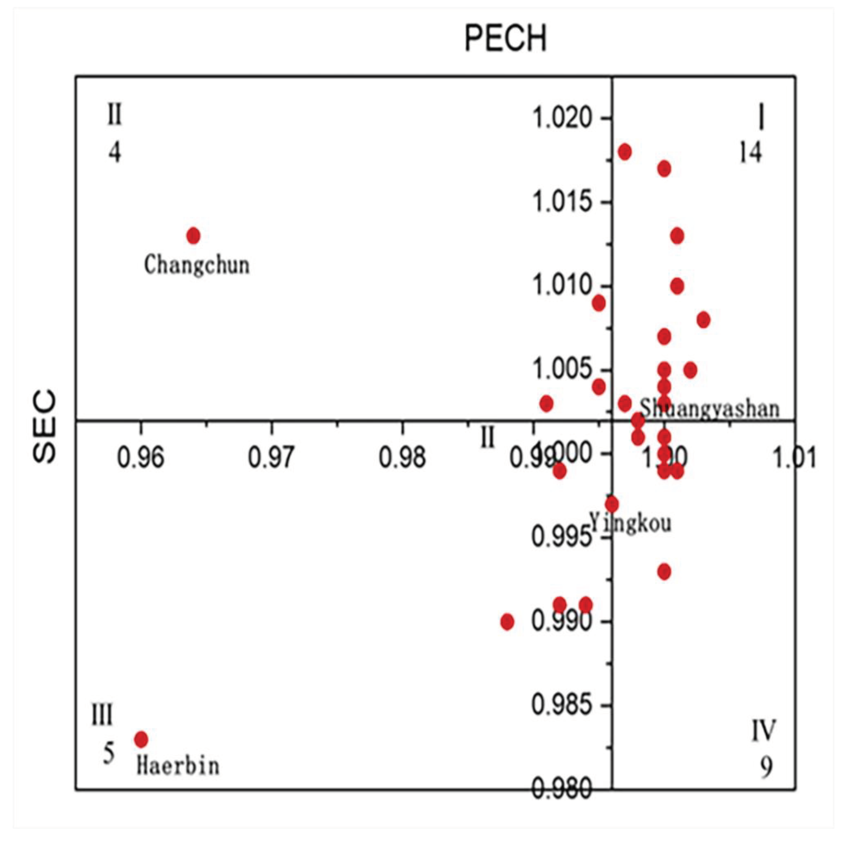
Based on the average values of pure technical efficiency and scale efficiency of 34 prefecture-level cities, the 34 prefecture-level cities in the three northeastern provinces were divided into four regions (Figure 8). Furthermore, targeted recommendations were proposed based on the characteristics of each region.

In Zone I, both technical efficiency and scale efficiency are greater than the average technical efficiency of prefecture-level cities as a whole. Water resource utilization is advantageous in the three provinces of the east, including 14 cities such as Shenyang, Liaoyang, and Heihe. These prefecture-level cities have good conditions and relatively high levels of water resource utilization. It is necessary for them to maintain their advantages, keep pace with the pace of technological iteration and updates, and ensure that their advantages continue to be exerted.

In Zone II, the scale efficiency is greater than the average level of 34 prefecture-level cities, but the technical efficiency is lower than the provincial average. It includes four cities: Anshan, Changchun, Fushun, and Yichun. For these cities, the key to improving water resource utilization lies in enhancing their own technological strength and improving their operational and management systems.

In Zone III, both technical efficiency and scale efficiency are relatively low. Compared with other cities, they are at a relatively backwards level. The five cities included Daqing, Jiamusi, Mudanjiang, Harbin, and Qiqihar. It is difficult for them to catch up with the preceding cities, so they need to reflect on whether their water resource planning and municipal expenditures are reasonable and formulate a reasonable development model. At the same time, they should also pay attention to improving their own technology, learn from other cities or advanced cities in terms of water resource utilization in China, and adopt new technologies to promote the improvement of water resource utilization.

In Zone IV, the technical efficiency is relatively high, but the scale efficiency is lower than the average level of the three northeastern provinces. This means that these cities may have problems with water supply and drainage in some areas. It is recommended to consider increasing investment in these areas, promoting regional rectification, rationalizing pricing and financial support, and improving the scale of water resource utilization.

Figure 8. The 34 prefecture-level cities in the three northeastern provinces are divided into four categories based on PTE and SE.

Figure 8. The 34 prefecture-level cities in the three northeastern provinces are divided into four categories based on PTE and SE.

4.3. Spatial Autocorrelation Analysis of Water Resource Utilization Efficiency

The spatial clustering of static water resource efficiency in the Northeast Region was explored using Geoda software (Table 5). Overall, the static water resource efficiency in the three provinces of the Northeast Region did not exhibit significant spatial clustering every year. This study examined the spatial significance of the water resource utilization rates in the three provinces from 2003 to 2020 (Table 6) and revealed that the significance of recent spatial clustering decreased compared to that in previous years.

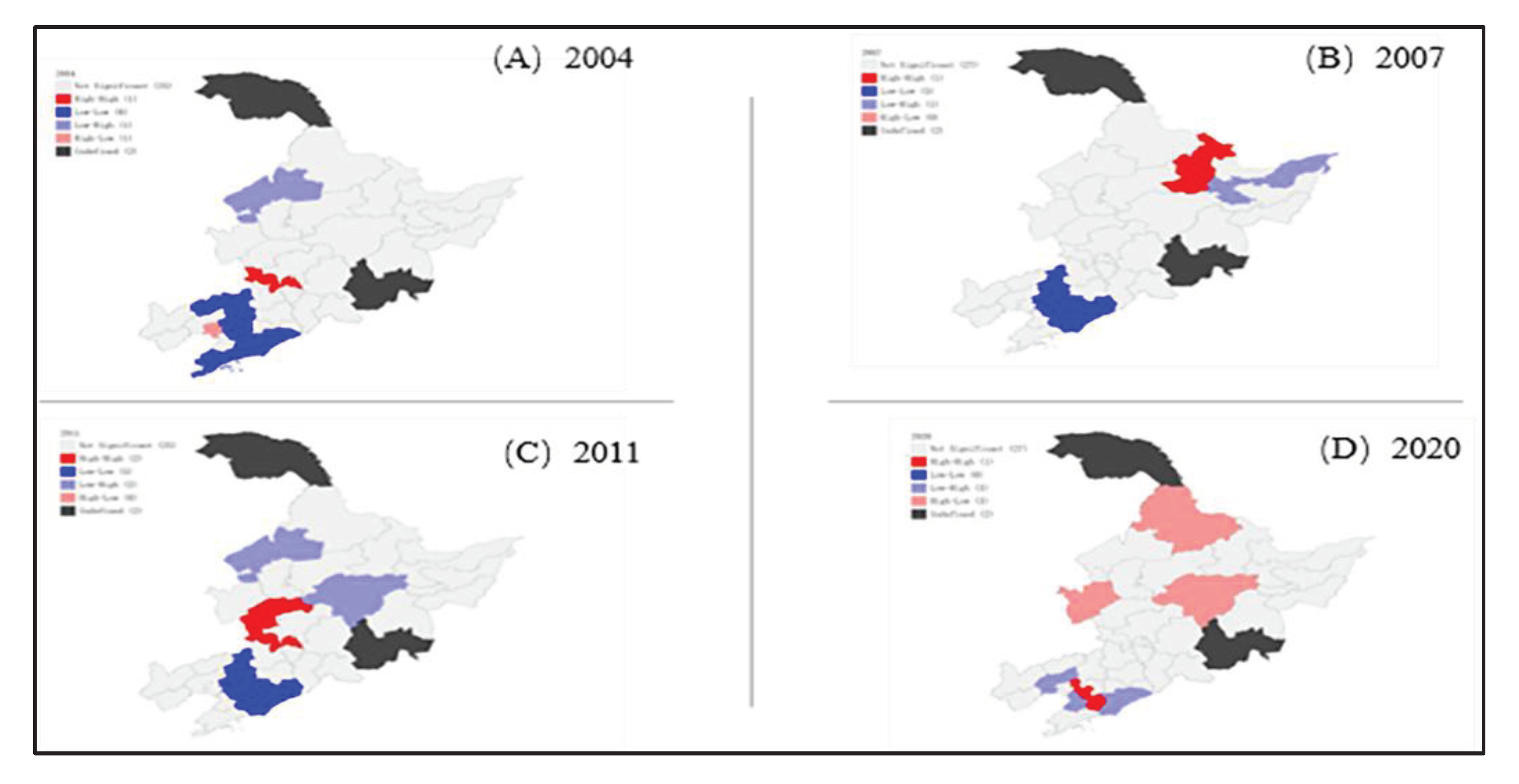
At a confidence level of 95%, the local spatial autocorrelation of the three provinces in the Northeast Region was observed, and the changes in spatial clustering were examined at 5-year intervals. It was found that there was an improvement in the spatial clustering of water resource utilization, transitioning from low-low clustering to high-low clustering and high-high clustering areas. This indicates that the scale effect of cities is gradually taking effect. Some cities have recognized the importance of water resource utilization, continuously improving water resource utilization rates, and generating regional effects that drive the improvement of water resource utilization efficiency in surrounding areas.

Table 5. List of significant years in the global Moran index of the three northeastern provinces.

Years Index	2004	2007	2011
Moran's I	0.223	0.196	0.153
Z Score	2.161	2.074	1.584
P Value	0.027**	0.037**	0.069*
Note: * Distinguish significance, * * * P<0.001, indicating very significant ** P<0.05 is more significant, * P<0.1 is more significant

Table 5. List of significant years in the global Moran index of the three northeastern provinces.

Years Index	2004	2007	2011
Moran's I	0.223	0.196	0.153
Z Score	2.161	2.074	1.584
P Value	0.027**	0.037**	0.069*
Note: * Distinguish significance, * * * P<0.001, indicating very significant ** P<0.05 is more significant, * P<0.1 is more significant

Figure 9. Local spatial autocorrelation analysis of the three northeastern provinces in 2005 (A), 2010 (B), 2015 (C), and 2020 (D).

Figure 9. Local spatial autocorrelation analysis of the three northeastern provinces in 2005 (A), 2010 (B), 2015 (C), and 2020 (D).

5. Analysis of Influencing Factors

A Tobit regression model was employed to investigate the factors influencing static water use efficiency in 34 prefecture-level cities located in the three northeastern provinces. Model 1 represents the regression model without considering control variables, while Model 2 includes time control variables in addition to Model 1 [32,33]. The outcomes are presented in Table 6, which indicates that the industrial structure, education level, overall economic expenditures of society, and GDP growth significantly impact changes in static water use efficiency.

The studies by Wenjing Qian and Canfei He [34], Yazong Buy [35], and Yufen Ren and Xiaowan Su [36] support the positive impact of industrial structure on water use efficiency. The water utilization efficiency in the three northeastern provinces is closely linked to the technological progress index. The elimination of outdated waste industries and the active development of high-tech industries can improve water utilization efficiency.

The findings of Yang Chao and Wu Lijun [37] as well as Zhao Liangshi [38] provide supporting evidence that education has a significant positive effect on water utilization. Education plays a crucial role in instilling water conservation among young students and enables higher-level students to apply their knowledge towards enhancing and optimizing water resource utilization techniques. As a result, this contributes to the overall enhancement of water resource utilization efficiency [26].

Socioeconomic expenditures have a significant deleterious effect on water use efficiency. To address the challenge of urban water utilization, it is necessary to augment financial expenditures and embrace the path of sustainable development. It would be beneficial to establish dedicated funds for enhancing water resources, as this would positively impact the lives of residents and foster the advancement of local industries in the three eastern provinces.

After accounting for control variables, it is observed that the GDP growth rate has a slight negative effect on water utilization. This implies that when the GDP growth rate is excessively rapid, the efficiency of water utilization in urban areas may decline. This can be attributed to the fact that an increase in GDP growth may result in a greater discharge of industrial wastewater, subsequently causing a reduction in water utilization. Therefore, while enhancing the input indicators of urban water utilization, emphasis should be placed on promoting the development of green industries and reducing the generation of unintended outputs.

Table 7. Tobit regression analysis of the water resource utilization rate in the three northeastern provinces.

Model 1					Model 2
Et_Vt	Coef.	Std. Err.	z	P>z	Et_Vt	Coef.	Std. Err.	Z	P>z
GDP growth rate	-0.31***	0.09	-3.31	0.001	GDP growth rate	-0.07	0.11	-0.68	0.49
Industrial structure	0.02	0.02	1.04	0.297	Industrial structure	0.04**	0.02	2.84	0.01
Open to the outside world	0.00	0.00	0.29	0.768	Open to the outside world	0.00	0.00	-0.80	0.43
Educational level	0.12	0.82	0.14	0.886	Educational level	3.86***	1.30	2.98	0.00
Socioeconomic expenditures	-0.18	0.18	-0.98	0.328	Socioeconomic expenditures	-1.07***	0.20	-5.23	0.00
_cons	0.81	0.09	9.02	0	_cons	0.52	0.15	3.50	0.00
Note: * Distinguishes significance, ***P<0.001 for highly significant, **P<0.05 for more significant, *P<0.1 for more significant.

Table 7. Tobit regression analysis of the water resource utilization rate in the three northeastern provinces.

Model 1					Model 2
Et_Vt	Coef.	Std. Err.	z	P>z	Et_Vt	Coef.	Std. Err.	Z	P>z
GDP growth rate	-0.31***	0.09	-3.31	0.001	GDP growth rate	-0.07	0.11	-0.68	0.49
Industrial structure	0.02	0.02	1.04	0.297	Industrial structure	0.04**	0.02	2.84	0.01
Open to the outside world	0.00	0.00	0.29	0.768	Open to the outside world	0.00	0.00	-0.80	0.43
Educational level	0.12	0.82	0.14	0.886	Educational level	3.86***	1.30	2.98	0.00
Socioeconomic expenditures	-0.18	0.18	-0.98	0.328	Socioeconomic expenditures	-1.07***	0.20	-5.23	0.00
_cons	0.81	0.09	9.02	0	_cons	0.52	0.15	3.50	0.00
Note: * Distinguishes significance, ***P<0.001 for highly significant, **P<0.05 for more significant, *P<0.1 for more significant.

6. Conclusions

In this study, we evaluated the water resource efficiency of 34 prefectural-level cities in the three eastern provinces. We also analysed the spatial correlation of water resource use efficiency in the three northeastern provinces over different time periods. Additionally, we investigated the factors that contribute to variations in water resource use efficiency. The following section presents our findings and provides corresponding recommendations:

(1) The spatial distribution of terrestrial water resources in the three northeastern provinces of China, i.e., Liaoning, Jilin, and Heilongjiang, is characterized by a greater quantity in the north and a lower quantity in the south, with more storage in spring and summer and less in autumn and winter. The seasonal differences are not significant. Overall, the utilization rate of static water resources in the three provinces is relatively good, with a high proportion of cities showing high and medium water resource utilization efficiency. However, there is still room for improvement in some areas. The distribution of cities with efficient water resource utilization is scattered, which hinders the realization of economies of scale. Southern cities have a more balanced distribution than do northern cities. The overall dynamic water resource efficiency of prefecture-level cities in the three northeastern provinces is good, and it is more consistent with the efficiency index of technological progress. Therefore, emphasis should be placed on the application of technology to improve water resource utilization.

(2) Different regions in the three northeastern provinces of China have varying factors that limit the development of water resources; therefore, it is necessary to improve their own water resource utilization according to local conditions. Of the total number of cities, 41.18% of the cities have advantageous water resource utilization efficiency, and 14.71% of the cities have achieved or surpassed the average level of water resource efficiency in the three provinces through scale efficiency. The key to improving water resource utilization lies in pure technological efficiency. A total of 29.41% of the cities need to improve their scale efficiency to enhance their own water resource utilization efficiency. This requires increased investment in funds and production supply scale. Additionally, 14.71% of the cities have lower water resource utilization efficiency than the provincial average. In these cases, increasing investment and expanding scale should be accompanied by a focus on improving their own technological capabilities.

(3) The spatial clustering of dynamic water resource utilization efficiency in prefecture-level cities in the three northeastern provinces is not strong, but over a longer time period, there has been a slight increase in spatial agglomeration. The main manifestation is the transition from low-low agglomeration to high-low agglomeration and high-high agglomeration. Areas with high water resource utilization efficiency have shown some growth, indicating a gradual increase in attention to water resource utilization.

(4) Water resource utilization efficiency is greatly influenced by industrial structure and education level. It is advisable to actively improve outdated industries and develop high-tech industries. At the same time, schools should implement water-saving awareness and behavior among students, cultivate water conservation consciousness, actively introduce professional talent, and contribute to the improvement of water resource utilization. Water resources are negatively affected by various social and economic expenditures. In the future, greater investment should be considered in improving water resource utilization efficiency, promoting the development of green industries, and pursuing sustainable development.

References

- Q. F. Wu. Attribution Analysis of Terrestrial Water Storage and Estimating Groundwater Recharge at Regional Scale on The Loess Plateau [D]. Northwest Agriculture and Forestry University of Science and Technology.
- F. Gong ; L.T. Du ; C. Meng ; Y. Dan ; L.Wang ; Q. Q. Zheng ; L. L. Ma ; Characteristics of water use efficiency in terrestrial ecosystems and its influence factors in Ningxia Province[J]. Journal of Ecology, 2019(24 vo 39): 9068-9078. [CrossRef]
- C. Z. Sun , K. Jiang , L. S. Zhao , Study on the measurement and spatial pattern of green efficiency of water resources in China[J]. Journal of Natural Resources,2017,32(12):1999-2011. [CrossRef]
- H. Q. Zhang , Y. L. Huang ; T. Qin , J. Li , Green efficiency of industrial water resources considering unexpected output based on SBM-Tobit regression model [J]. Water Economics, 2019(05 vo 37): 35-40+47+78-79.
- Z. Zhou , H. Wu , P. Song , Measuring the Resource and Environmental Efficiency of Industrial Water Consumptionin China: A Non-Radial Directional Distance Function[J]. Journal of Cleaner Production, 2019(240): 118169. [CrossRef]
- L. Yue , Y. Y. Lei , Construction of Spatial Linked Network of Green Water Resource Efficiency in the Yellow River Basin and its Evolutionary Factors [J/OL]. Journal of Northwest Normal University (Social Science Edition), 2022(02 vo 59): 62-74.
- T. Deng , D. Wang , Y. Yang , et al. Shrinking cities in growing China: Did high speed rail further aggravate urban shrinkage? [J/OL]. Cities, 2019,210-219. [CrossRef]
- G. S. Yang, Q. H. Xie, Study on the spatial and temporal differentiation of green water resources efficiency in the Yangtze River Economic Belt [J]. Yangtze River Basin Resources and Environment, 2019(02 vo 28): 349-358.
- M. F. Gao ,H. Yu , J. Zheng. Research on green water efficiency and spatial drivers in the Yellow River Basin[J]. Ecological Economy,2020,36(07):44-50+209.
- Li Jian,Xie Heng. Analysis of green water utilization efficiency and its spatial and temporal differences and drivers in Beijing-Tianjin-Hebei[J]. Journal of Water Resources and Water Engineering,2021,32(06):10-18.
- Sun Qian. Research on spatial and temporal changes of water resources in Xinjiang based on GRACE and GLDAS [D]. Xinjiang University,2016.
- LUO Zhicai,LI Qiong,ZHONG Bo. Inversion of water storage changes in the Heihe River Basin using GRACE time-varying gravity field[J]. Journal of Surveying and Mapping,2012,41(05):676-681.
- Tiwari V M, Wahr J and Swenson S. Dwindling groundwater resources in northern India[J]. from satellite gravity observations, 2009(36): L18401. [CrossRef]
- LI Qiong,LUO Zhicai,ZHONG Bo et al. Detection of water storage changes in arid land of southwest China in 2010 using GRACE time-varying gravity field[J]. Geophysical Journal,2013,56(06):1843-1849.
- SONG Guojun,HE Wei. Benchmarking of water resource utilization efficiency in Chinese cities[J]. Resource Science,2014,36(12):2569-2577.
- CHEN Yanping,LIU Chang. Water resource utilization efficiency and its spatial and temporal differentiation characteristics in the Yellow River Basin[J]. Statistics and Decision Making,2022,38(08):62-66.
- SUN Caizhi,XIE Wei,JIANG Nan et al. Spatial and temporal variability of the relative efficiency of water resources utilization in China and the factors affecting it[J]. Economic Geography,2010,30(11):1878-1884.
- Jin Wu,Yang Wei. Analysis of the current situation and rational utilization of water resources in northeast China[J]. Heilongjiang Science and Technology Information,2015(28):182.
- Wang Jiaze. Study on the Measurement of Sustainable Development Level of Water Resources in Northeast China[D]. Jilin University of Finance and Economics,2020.
- Cui L, Zhang C, Luo Z, et al. Using the Local Drought Data and GRACE/GRACE-FO Data to Characterize the Drought Events in Mainland China from 2002 to 2020[J/OL]. Applied Sciences-Basel, 2021, 11(20): 9594. [CrossRef]
- ZHOU Zejiong,HU Jianhui. Research on performance evaluation of low-carbon economic development based on Super-SBM model[J]. Resource Science,2013,35(12):2457-2466.
- Tone K. A slacks-based measure of efficiency in data envelopment analysis[J/OL]. European Journal of Operational Research, 2001, 130(3): 498-509. [CrossRef]
- Tone K. A slacks-based measure of superefficiency in data envelopment analysis[J/OL]. European Journal of Operational Research, 2002, 143(1): 32-41. [CrossRef]
- Liu K, Xue Y, Lan Y, et al. Agricultural Water Utilization Efficiency in China: Evaluation, Spatial Differences, and Related Factors[J/OL]. Water, 2022, 14(5). [CrossRef]
- SUN Caizhi,MA Qifei,ZHAO Liangshi. Research on the change of green efficiency of water resources in China based on SBM-Malmquist productivity index model[J]. Resource Science,2018,40(05):993-1005. [CrossRef]
- Wang S, Zhou L, Wang H, et al. Water use efficiency and its influencing factors in China: based on the data envelopment analysis (dea)-tobit model[J]. 2019.
- Kumar K S, Anandraj P, Sreelatha K, et al. Monthly and Seasonal Drought Characterization Using GRACE-Based Groundwater Drought Index and Its Link to Teleconnections across South Indian River Basins[J]. Climate, 2021, 9(4): 56. oi.org/10.3390/cli9040056.
- Liu K, Yang G liang, Yang D gui. Industrial water-use efficiency in China: Regional heterogeneity and incentives identification[J/OL]. Journal of Cleaner Production, 2020, 258: 120828. [CrossRef]
- Wang S, Gao S, Huang Y, et al. Spatiotemporal evolution of urban carbon emission performance in China and prediction of future trends[J]. Journal of Geographical Sciences, 2020, 30(5): 18.
- Zhong K, Wang Y, Pei J, et al. Super efficiency SBM-DEA and neural network for performance evaluation[J/OL]. Information Processing & Management, 2021, 58(6): 102728. [CrossRef]
- ZHANG Zhaofang,SHEN Juqin,HE Weijun et al. "Evaluation of regional water resources utilization efficiency in Belt and Road China - based on superefficient DEA-Malmquist-Tobit method[J]. Journal of Hohai University (Philosophy and Social Science Edition),2018,20(04):60-66+92-93.
- Feng L , Wang L , Zhou W .Research on the Impact of Environmental Regulation on Enterprise Innovation from the Perspective of Official Communication[J].Discrete Dynamics in Nature and Society, 2021.
- Wang S, Zhou L, Wang H, et al. Water Use Efficiency and Its Influencing Factors in China: Based on the Data Envelopment Analysis (DEA)-Tobit Model[J/OL]. Water, 2018, 10(7): 832. [CrossRef]
- QIAN Wenjing,HE Canfei. Study on regional differences in China's water resources utilization efficiency and influencing factors[J]. China Population-Resources and Environment,2011,21(02):54-60.
- BAI Yazong, SUN Fuli, HUANG Linglang et al. Assessment of water resources utilization efficiency and regional differences in China[J]. Environmental Protection Science,2014,40(05):1-7.
- REN Yufen,SU Xiaowan,HE Yuxiao et al. Urban water utilization efficiency and influencing factors in China's eco-geographical zones[J]. Journal of Ecology,2020,40(18):6459-6471.
- YANG Chao,WU Lijun. Differential analysis of water resources utilization efficiency in Chinese cities - Empirical evidence based on panel data of 286 prefecture-level and above cities[J]. People's Yangtze River,2020,51(08):104-110.
- ZHAO Liangshi, SUN Caizhi, ZHENG Defeng. Measurement of interprovincial water utilization efficiency and spatial spillover effects in China[J]. Journal of Geography,2014,69(01):121-133.