Submitted:
28 March 2024
Posted:
28 March 2024
You are already at the latest version
Abstract
Two strongly curved areas of the Carpathians in Romania are earthquake-prone: Vrancea - in the South-Eastern Carpathians, and Danubian – in the western edge of the Southern Carpathians. By far the highest seismicity episode in 2023 was recorded in the Southern Carpathians, near Targu Jiu city, of more than 4000 earthquakes. A first ML 5.2 mainshock was recorded on 13 February, followed by a second one, ML 5.7, on 14 February. Our purpose is to provide a first analysis of this sequence in order to explain its extent and unusual development, in time. The possible role of fluids in the middle crust, is discussed in connection with the rather unusual character of the space-time distribution of aftershocks. A large and high-quality dataset is provided by the dense array of seismic stations which has been gradually improved by adding new stations in the epicentral area. The thorough revision of the phase picking and location reveals a few interesting and intriguing features of seismicity that still remain worthy to be further investigated. The database built within this paper provides excellent information not only for Targu Jiu area, but for any other investigation in intra-continental regions characterized by diffuse and sporadic seismic activity.
Keywords:
intra-continental seismicity
; Southern Carpathians (Romania)
; earthquake sequence
; seismicity pattern
; JHD location
1. Introduction
The Carpathians mountain footprint in Romania currently shows two strong bends, one in the Vrancea region, at the southern end of the Eastern Carpathians and the other at the south-western segment of the Southern Carpathians, where the orogenic chain rotates towards Danube river. Both areas of curvature are associated with enhancement in seismicity. While the first zone is well known for its intense and concentrated seismic activity with frequent events of magnitude above 7 at intermediate depths, due to a complex and geodynamically active collisional system (e.g., [1]), the seismicity in the second zone is significantly weaker (events with magnitude less than 6), more diffuse and limited to the crustal domain. For this reason, the seismologists paid much more attention to what is happening in the Vrancea area than in the other earthquake-prone areas located along the Southern Carpathians and adjacent regions.
However, by far the highest seismicity episode in 2023 was recorded in the Southern Carpathians, near Targu Jiu city, when an earthquake sequence of more than 4000 events has been recorded. The ML 5.2 mainshock on 13 February, at 14:58 (GMT), was followed by a second large shock, ML 5.7, on 14 February, at 13:16. The purpose of this work is to provide a first analysis of this sequence in order to explain its extent and unusual development, during a time span of about one year.
The area under study is located in the Getic Depression, located southward of the Southern Carpathians. The Getic Depression is bounded to the south by the Pericarpathian Fault that separates it from the western segment of the Moesian Platform (Figure 1). This segment of the Moesian Platform is largely aseismic, at least on the time scale for which we have earthquake data available. The only area with potential to generate earthquakes with a magnitude above 4 is the contact area of the Getic Depression with the Southern Carpathians. The seismicity there is moderate and characterizes an intraplate region. We find sporadic information about the seismicity of the area starting with the 20th century. The largest recorded earthquakes before 2023 did not exceed magnitude 6: 23 June 1900 07:06 (Mw = 4.2), 9 July 1912 21:46 (Mw = 4.5), 20 June 1943 01:00 (Mw = 5.2), 4 May 1963 16:48 (Mw = 4.5) and 1 January 2012 23:57 (Mw = 4.5). A relatively intense man-made activity (quarry blasts) practically coincides with the tectonic activity [2]. Due to this contamination, the analysis of the activity of small earthquakes has become difficult in the last years.
A spectacular increase in seismic activity was registered during 2023, when three events with local magnitude ML ≥ 5 were recorded, accompanied by more than 4000 aftershocks. This burst of activity in the area is far beyond what was known until now and more than likely reflects a process of accumulation of deformation on a larger scale compared to the scale of observable data that we are aware of.
The catalogue existing until this work is a routine version based on the Antelope software for a global model (IASP91, [3]). The procedure adopted to build the catalogue is the one routinely applied to obtain the Romanian earthquake [4]. A first version of the catalogue can be found in the database published in Mendeley [5], which contains the events recorded until 22 March 2023, and which is in process of being updated.
In a preliminary analysis of the catalogue data, [6] showed how artificial biases can be generated among locations when the configuration of the network stations changes. At the same time, the authors recommended to use group localization techniques to overcome these inadvertences.
2. Materials and Methods
The current catalogue data were reconsidered in the paper by systematically reading and revising of P and S phases, reaching this way an improved and complete catalogue version containing all the localised events recorded between February 13 and October 30, 2023 (4015 events with local magnitudes between around 0 and 5.7). Note that the configuration of the stations used in the detection and localization of earthquakes underwent several improvements as the seismic activity evolved over time. Particularly the introduction of additional stations in the epicentral area contributed to the increase of the localization accuracy and the significant decrease of the minimum magnitude threshold. Thus, after the sequence was triggered, the National Institute for Earth Physics (NIEP) of Magurele (Romania) installed five additional seismic stations in the epicentral area: LELR on 15 February, DBRR and PTSR on 16 February, BVPR on 22 February and CPSR on 3 June, 2023. Depending on the configuration of the seismic stations in operation, we can consider five stages in the localization of earthquakes:
1) 13 February, 14:58 – 15 February, 20:24;
2) 15 February, 20:41 – 16 February, 20:27 - one additional station (LELR) in the epicentral area;
3) 16 February, 20:56 - 21 February, 23:58 two additional stations (DBRR, PTSR) in the epicentral area;
4) 22 February, 00:03 – 3 June, 03:04 one additional station (BVPR) in the epicentral area;
5) 3 June, 18:46 – 23 October, 19:08 one additional station (CPSR) in the epicentral area.
Taking into account the bias effects in location reported by [6], we carried out location analyses separately for each stage using both routine and Joint Hypocentre Determination (JHD) techniques.
The JHD technique was first proposed by [7] and then developed by numerous researchers [8,9,10,11]. The principle of the method consists in the simultaneous localization of a set of events, taking into account the lateral variations of the structure transversed by the seismic rays and determining a common set of corrections for travel times for each station. Taking into account the complexity of the Earth’s structure in the studied area and the distribution of the seismic stations, we consider that the use of the JHD localization technique can be a benefit for obtaining source locations with the smallest possible errors.
An important factor to obtain high-precision localizations is the use of an optimised local velocity model, as close as possible to the real structure crossed by the rays from the source to the stations. In our analysis, we selected a 1-D velocity model which is a combination of the models developed by [12] and [13] for the south-western part of Romania (Table 1).
3. Results
3.1. Location Investigation
As shown before, significant biases in location can be generated by different station configurations when using absolute location techniques. To measure how large these effects are, we performed an analysis for the five stages characterized by different configurations of stations in the epicentral area. We analysed in parallel the routine locations with the JHD ones.
The first interval includes the activity recorded between the first two shocks with magnitude above 5 (M1 on 13 February, 14:58 of magnitude ML 5.2 and M2 on 14 February, 13:16 of magnitude ML 5.7) followed by the events recorded until 15 February 20:24, 57 events in all (Figure 2a). Comparing the routine locations vs JHD locations, we notice a distinct shift in space between them, and a mismatch between the position of the main shocks (M1 and M2) and the position of the aftershocks for routine locations (black symbols), while for JHD locations (pink symbols) this shortcoming does not appear. As shown by [6], this may be an effect due to the different distribution of stations used in location, more precisely the different weight of distant stations vs close stations for events where the magnitudes differ significantly.
Another interesting aspect revealed in the figure refers to the way the activity evolved after the M1 shock was triggered. The aftershocks occurred toward NW, while the second shock (M2) is situated in the opposite direction relative to M1. This makes us assume that M2 was caused by a sudden stress variation following the triggering of M1 and not by a directivity effect that we would have expected if the rupture of M1 source had propagated towards SE.
Epicentres distribution in the second stage are plotted in the Figure 2b. A number of 590 earthquakes was recorded and located within one day of this stage. A new station (LELR) came into operation. The aftershocks of the first two main shocks propagated along ENE – WSW direction, which fits well the geometry of the nodal planes in the fault plane solutions of the main shocks (GFZ solution, [14]). Similar results were obtained by [15] who determined focal mechanisms for the 51 earthquakes with ML>2.9, based on the first motion of P-wave polarities. The fault plane solutions show in general a normal faulting oriented roughly in the ENE-WSW direction.
In the next stage (Figure 2c), two additional stations became operational in the epicentral area: DBRR and PTSR. Note that the discrepancy between routine and JHD locations is reduced for the new configuration of stations. The considerable increase in the density of epicentres near the future major shock M3 is also noticeable. The number of detected and located events remains high (418) due to the increase in the number of stations and implicitly to the increase of the detection and localization capacity.
The number of detected and located events increases considerably in the next stage (2195 events) when a new station (BVPR) was installed close to the epicentral area (Figure 2d), also due to the long duration of this stage. During this period the last major shock of magnitude ML5.0 was recorded (on 20 March 14:02). Considering the migration in time of the seismicity (revealed in the previous figures), it is obvious that this shock was caused by the stress increase as a result of the propagation of the activity towards WSW.
The epicentres distribution in the last stage is plotted in Figure 2e. The CPSR additional seismic station started operating in this stage. The station was installed in close proximity to the epicentres of the two shocks M1 and M2. The largest earthquakes of magnitude ML ≥4.0 occurred on 19 June, 05:26 (ML = 4.3), 18 July, 20:30 (ML = 4.4) and 20 August, 21:33 (ML = 4.5), plotted by blue stars in the figure. The last one is located somewhat outside the active area and it remains to be clarified to what extent it is triggered by the ongoing sequence or not. A closer look to the figure suggests a possible migration of the activity from the ENE - WSW direction to a perpendicular direction that could be interpreted as an activation of a secondary fault.
The comparative inspection of the locations using the Antelope program applied routinely for the NIEP catalogue ROMPLUS using IASP91 global model and the JHD program using the optimised local model outlines a few important features:
- -
- -
- JHD locations are practically not influenced by the differences in stations configuration as Antelope locations do. Note, however, that as the number of stations in the epicentral area increases, both the systematic shift in space and the hypocentres dispersion for routine locations come closer to the JHD results (compare the epicentres distribution in the first stages with those in the final stages; also, the depth distribution as shown in the first and in the last histograms);
- -
- Location errors, illustrated by the histograms of the RMS values (Figure 4) are significantly reduced when using JHD locations.
As concerns the location error (RMS), we emphasise from the Figure 4: (i) the increase in location accuracy with the improvement of the seismic network configuration, which is found both at routine locations and at JHD ones, which was to be expected and (ii) a systematic decrease in the RMS values for JHD as compared with Antelope in any of the five configurations (a difference of about 0.25 s).
3.2. Quarry Activity: Possible Triggering Effects?
It is worth mentioning that the two main shocks M1 and M2 occurred just close to a quarry site (Dobriţa). We identified three quarries which are presently active in the area: Bumbeşti-Jiu, Dobriţa (Susesni) and Pestişani (Figure 5). Bumbeşti-Jiu and Pestişani quarries appear to be inactive or the detonation level is too low to be detected with acceptable signal/noise ratio by the seismic stations in the region, while the Dobrița quarry activity is relatively well monitored.
If we examine the seismic activity recorded before the triggering of the sequence, we notice a concentration of epicentres in the area around the quarry site (marked by an ellipse in the figure). This enhancement of activity can be explained by anthropic activity. On the other hand, the area affected by the seismicity that precedes the sequence roughly delimits the area of the future earthquake sequence. It means that in our opinion the preceding seismicity is somehow related to the seismicity in the sequence.
The analysis of day-night distribution of the events illustrated in Figure 6, which shows a strong concentration of events generated during day-time clustered around Dobrița quarry site. For the day-time we used the time interval from 7 to 16, and the night-time for the rest of the day. The inhomogeneous distribution throughout the day is a clear indication that we are dealing with human activity.
The coincidence of the epicentral area with the quarry exploitation site is certainly intriguing and can lead us to think of a possible triggering effect. However, a calculation of the typical energy release in the case of a quarry blast and the energy released by a magnitude 5 earthquake shows a difference of about 30,000 times. In addition, the explosions are generated in close proximity to the Earth’s surface and it is known that in this case the energy dissipates rapidly as the generated waves propagate at distance.
Another interesting aspect is revealed when comparing Figure 5 with Figure 2: the migration of epicentres of the aftershocks from east to southwest and the dimension range on which this migration takes place seem to be anticipated by the activity preceding the sequence. Since the probability that the amount of quarry activity, even over a long time period, is capable of perturbing the tectonic stress accumulation at the seismogenic depth range is negligible, we are tempted to attribute the above-mentioned coincidental aspects simply to chance. Maybe, in future approaches, we should take into account more subtle processes able to destabilise an area that is very sensitive to small and repeated disturbances.
3.3. Wadati Analysis
Wadati diagram provides a simple way to estimate the mean of the VP/VS ratio characterizing the region where the sequence was recorded. If the geological structure were homogeneous, the ratio obtained would have the same value for the data recorded at any seismic event. We applied the modified Wadati diagram based on double-difference arrival times, as proposed by [16]. VP/VS ratio is given by the slope of the straight line that best fits the difference between couples of tSi- tSj travel times for S waves vs. couples of tPi- tPj travel times for P waves, where the couples (i,j) refer to the stations which recorded both P and S waves for each event. This method allows the use of all the pairs of travel times for P and S waves available for all events in the catalogue in a single diagram because these pairs do not depend on the origin time of each event.
The analysis of Wadati distribution performed on different sets extracted from the catalogue shows up two significant features:
- -
- VP/VS ratio is systematically lower when considering readings for stations located within 100 km distance from epicentre;
- -
- VP/VS ratio is almost exclusively below the theoretical level (1.73).
We show in Figure 7 examples of Wadati diagram for two sets of earthquakes, one recorded at the beginning of the sequence (304 events occurred between 13 February 14:58 and 16 February 07:15) and the other recorded at the end of the sequence (295 events occurred between 7 July 01:15 and 24 October 19:01). Note that the slope of the best fitting line is smaller than 1.73 value, both for the entire network and near-epicentral network. In Figure 7 we tested if VP/VS ratio is stable over time or suffers significant variations.
The first point on the plot corresponds to the set of events preceding the sequence. The number of events per set varies from 4 (at the beginning) to 30 events (at the end). We mention that modifying the selected windows (for example, selecting a constant number of events per window) does not essentially change the results presented in Figure 8. Note that at the beginning of the sequence the slope inferred from the readings for the entire seismic network are close to 1.73 (first three black dots). As the time runs, the values systematically decrease below the theoretical value. There are only a few sets with VP/VS > 1.73. As regards the slopes estimated from the readings from the epicentral stations (red dots), they are always below 1.73 (effectively, they extend over 1.6 – 1.7 interval). If the fluctuations are attributed to statistical errors, we can conclude that the ratio VP/VS is really stable over time and that it is significantly lower than 1.73.
Considering the unusually long duration of the sequence (more than 8 months), we assume that destabilisation processes due to the presence of fluids should take place in the region. In this hypothesis, we would have expected the ratio VP/VS to be greater than 1.73. Clearly, our results contradict this expectation. Results similar to ours were reported for the mid-crustal (8–10 km) earthquake swarms recorded in the NW-Bohemia swarm region [17]. In case of several swarms generated in the region, an anomalous drop VP/VS to low values (as low as ~1.4) is explained by the presence of gases under high overpressure in the source zone. This implies an area with a high level of complexity in the relation between stress changes accompanying the seismogenic process and crustal fluids that are represented primarily by water and CO2 at seismogenic depth. If we assume that the rock there is fractured and can be represented by a porous model with small porosity, oversaturated gases can suddenly fill the pore space as a result of a spontaneous transition of fluid to gaseous phases. The source volume can be enriched in this way with a gaseous phase which tends to migrate upward as being buoyancy driven.
4. Discussion
The seismic activity along the Southern Carpathians in Romania is known as a typical intra-continental activity of moderate size and sporadic in time. Only a few events of magnitude over 5 have been reported in this region since we have information available. An unusual intensification of seismic activity was recorded all along 2023 in the area located NW of Targu Jiu. The activity started in February 2023 with a pair of earthquakes of magnitude above 5 generated one day apart from each other. This is by far the most intense episode of seismicity in the Southern Carpathians.
During the sequence (February - October 2023), various configurations of stations were used in localization, which create undesirable biases in the relative positions of the hypocentres: first, differences in larger events compared to smaller ones due to the fact that the station coverage differs a lot; then, the differences between the events in the first part of the sequence and those that later benefited from an increasing number of stations in the epicentral area. The analysis carried out by us shows that these effects are strong in routine locations, instead they decrease considerably in group localizations. It is also observed that the systematic mismatch in space found between routine and JHD locations decreases as the number of stations in the epicentral area increases. Thus, we tested on a rich data set the important weight of the presence of stations in the epicentral area to ensure highly accurate locations and, at the same time, the ability of group location techniques (JHD specifically) to reduce the unwanted effects caused by poor station configurations.
By revising the readings of P and S phases, we set up a catalogue containing all the localised events recorded between February 13 and October 30, 2023 (4015 events with local magnitudes between around 0 and 5.7). To get refined locations, we applied the JHD procedure using an optimised velocity local model. The hypocentral distributions reveal some notable space-time alignments of foci migration: (i) from lower crust (h ∼ 20 km) to upper crust (h ∼ 10 km) and (ii) from NE to SW. These migrations are in good agreement with the focal mechanisms that indicate reverse faulting in the NE-SW direction. At the same time, it is known that extensional mechanisms favour the migration of aftershocks towards the surface of the Earth. For the last stage of the sequence (after June 2023), there is a tendency of seismicity to migrate along a perpendicular direction (NW - SE), which could possibly be attributed to the existence of a secondary fault lying along this direction (Figure 2e).
The earthquake activity in the Targu Jiu area has continued even until the end of 2023. To explain such a long duration for a sequence generated by moderate shocks (magnitude below 6), we have to assume some specific driving mechanisms in connection with extensional tectonics and destabilisation processes. Long sequences of earthquakes have been reported quite often in Italy, when the stress regime was extensional as indicated by a predominant normal faulting regime as in our case. Crustal extensional settings may induce gravity-driven motion (so-called graviquakes, see [18], or opening of fractures allowing this way fluids migration and gradually weakening of the region. As shown by [19], the aftershocks of normal faults last longer than those of thrust faults. The differential stress necessary to generate rock failure is on average 5–6 times smaller than that required in contractional tectonic settings.
The presence of water at depth would lead, as expected, to an increase in the VP/VS ratio above the theoretical value (1.73), which is not observed in the Wadati analysis carried out by us. The ratio is systematically below this value throughout the sequence (Figure 7). Results similar to ours were reported for the mid-crustal (8–10 km) earthquake swarms recorded in the NW-Bohemia region [17]. For this case, the anomalous drop of VP/VS to low values (as low as ~1.4) is explained by the presence of gases under high overpressure in the source zone. This implies an area with a high level of complexity in the relation between stress changes accompanying the seismogenic process and crustal fluids that are represented primarily by water and CO2 at seismogenic depth. If we assume that the rock there is fractured and can be represented by a porous model with small porosity, oversaturated gases can suddenly fill the pore space as a result of a spontaneous transition of fluid to gaseous phases. The source volume can be enriched in this way with a gaseous phase which tends to migrate upward as being buoyancy driven. By analogy, we assume that the focal zone of the Targu Jiu sequence is characterized by a high level of complexity, with multiple fractures in the rock and with a degree of porosity that allows gases under pressure (coming from the spontaneous transition of deep fluids) to suddenly penetrate into the porous space. In this way, the conditions are created for a significant decrease in the VP/VS ratio compared to the normal value. In principle, this model would explain the results obtained in the paper, but the problem remains open for future investigations that call for geotectonic arguments in addition to seismic analyses.
Supplementary Materials
The catalogue of events located using JHD can be downloaded at.
Author Contributions
Conceptualization, M.R. and B.E.; data curation, A.C., R. D., M. P., M.R.; methodology, M.P.; software, M.R., M.P.; validation, A.C., R.D., M.P., B.E; formal analysis, M.R.; investigation, A.C.; resources, A.C.; writing—original draft preparation, M.R., M.P., B.E.; writing—review and editing, M.R., M.P., B.E; visualization, R.D.; supervision, B.E.; project administration, M.R.; funding acquisition, M.R. All authors have read and agreed to the published version of the manuscript.
Funding
This research was funded by Ministry of Research, Innovation and Digitalization, grant number 2336, “Advanced research for the modeling of natural and anthropogenic phenomena in the Earth-Atmosphere coupled system in order to reduce associated risks” – SOL4RISC (2023 – 2026) and by the AFROS Project PN-III-P4-ID-PCE-2020-1361, 119 PCE/2021, supported by UEFISCDI, Romania.
Data Availability Statement
The existing database in Mendeley [5] is ready to be updated using the new catalogue.
Conflicts of Interest
The authors declare no conflicts of interest.
References
- Ismail-Zadeh, A.; Maţenco, L.; Radulian, M.; Cloetingh, S.; Panza, G. F. Geodynamics and intermediate-depth seismicity in Vrancea (The South-Eastern Carpathians): Current state-of-the art. Tectonophyiscs 2012, 530–531, 50–79. [Google Scholar] [CrossRef]
- Radulian, M.; Dinescu, R.; Popa, M. Earthquake prone areas in Romania. Annals of the Academy of Romanian Scientists 2019, 4, 107–164. [Google Scholar]
- Kennett, B.L.N.; Engdahl, E.R. Travel times for global earthquake location and phase association. Geophysical Journal International 1991, 105, 429–465. [Google Scholar] [CrossRef]
- Popa, M.; Chircea, A.; Dinescu, R.; Neagoe, C.; Grecu, B.; Borleanu, F. Romanian Earthquake Catalogue (ROMPLUS). Mendeley Data 2022, V2. [Google Scholar] [CrossRef]
- Armeanu, I.; Chircea, A.; Ciobanu, I.; Craiu, A.; Craiu, G. M.; Dinescu, R.; Mihai, M.; Predoiu, A.; Tolea, A.; Varzaru, L.-C.; Borleanu, F.; Neagoe, C.; Radulian, M.; Popa, M. Database of the 2023 seismic sequence recorded in Gorj area (Romania). Mendeley Data 2023, V1. [Google Scholar] [CrossRef]
- Radulian, M.; Popa, M.; Dinescu, R.; Bala, A. Location improvements for the twin crustal earthquakes recorded on 23 in Gorj county, Romania. Proceedings 23rd SGEM International Multidisciplinary Scientific GeoConference; 2023; vol. 23. [Google Scholar] [CrossRef]
- Douglas, A. Joint hypocenter determination. Nature 1967, 215, 47–48. [Google Scholar] [CrossRef]
- Herrmann, R.; Park, S.; Wang, C. The Denver earthquakes of 1967-1968. Bull. Seismol. Soc. Am. 1981, 71, 731–745. [Google Scholar] [CrossRef]
- Pavlis, G.; Booker, J. Progressive multiple event location (PMEL). Bull. Seismol. Soc. Am. 1983, 73, 1753–1777. [Google Scholar] [CrossRef]
- Pujol, J. Comments on the joint determination of hypocenters and station corrections. Bull. Seismol. Soc. Am. 1988, 78, 1179–1189. [Google Scholar] [CrossRef]
- Pujol, J. Joint event location – The JHD technique and applications to data from local seismic networks. In Advances in Seismic Event Location; Chapter 7; Thurber, C.H., Rabinowitz, N., Eds.; Kluwer Academic Publishers, 2000; pp. 163–204. [Google Scholar] [CrossRef]
- Raileanu, V. Geological characterization and elastic parameters of the sites of seismic and accelerometric stations sites of the INCDFP network. In Research on management of disasters generated by the Romanian earthquakes; Tehnopress: Bucharest, 2009; pp. 297–332. [Google Scholar]
- Zaharia, B.; Grecu, B.; Popa, M.; Oros, E.; Radulian, M. Crustal structure in the western part of Romania from local seismic tomography. In Proceedings of the World Multidisciplinary Earth Sciences Symposium WMESS 2017; Prague, IOP: Earth and Environmental Sciences. 2017; p. 95. [Google Scholar] [CrossRef]
- Available online: https://geofon.gfz-potsdam.de/old/eqinfo/list.php?mode=mt (accessed on 9 January 2024).
- Craiu, A.; Diaconescu, M.; Craiu, M.; Mihai, M.; Marmureanu, A. Stress field Targu Jiu seismotectonic area (Romania): insights from the inversion of earthquake focal mechanisms. 23rd International Multidisciplinary Scientific GeoConference SGEM 2023; 2023. [Google Scholar] [CrossRef]
- Chatelain, J.L. Étude fine de la sismicité en zone de collision continentale au moyen d’un réseau de stations portables: la région Hindu-Kush Pamir, Thèse docteur de 3e cycle, L’Université scientifique et médicale de Grenoble, 1978, 219 pp.
- Dahm, T.; Fischer, T. Velocity ratio variations in the source region of earthquake swarms in NW Bohemia obtained from arrival time double-differences. Geophysical Journal International 2014, 196, 957–970. [Google Scholar] [CrossRef]
- Doglioni, C.; Carminati, E.; Petricca, P.; Riguzzi, F. Normal fault earthquakes or graviquakes. Sci. Rep. 2015, 5, 12110. [Google Scholar] [CrossRef]
- Valerio, E.; Tizzani, P.; Carminati, E.; Doglioni, C. Longer aftershocks duration in extensional tectonic settings. Scientific Reports 2017, 7, 16403. [Google Scholar] [CrossRef]
Figure 1.
The seismotectonic framework. Epicentre locations are from the Romanian catalogue (ROMPLUS) using the stations of the Romanian Seismic Network (RSN).
Figure 1.
The seismotectonic framework. Epicentre locations are from the Romanian catalogue (ROMPLUS) using the stations of the Romanian Seismic Network (RSN).
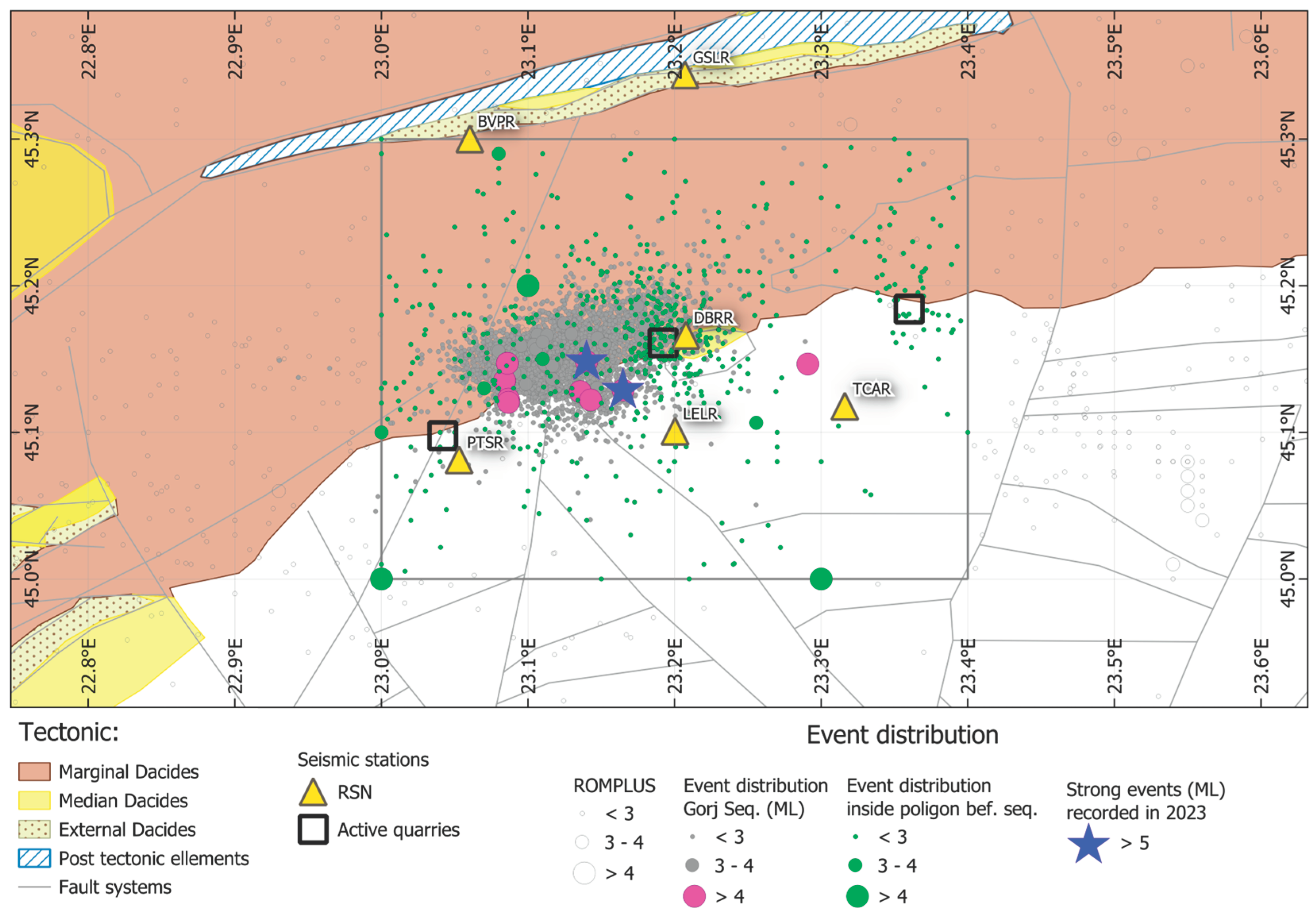
Figure 2.
Distribution of epicentres: a. Stage 1 (13 February 14:58 – 15 February 20:24). The main shocks with magnitude ML ≥ 5.0 are plotted with stars (including M3 which was produced later): black and pink stars routine and JHD locations, respectively; b. Stage 2 (15 February, 20:41 – 16 February, 20:27). A new seismic station (LELR) came into operation at this stage. Fault plane solutions in the upper-right side are computed by GFZ; c. Stage 3 (16 February, 20:56 – 21 February, 23:58). Two new seismic stations (DBRR and PTSR) came into operation at this stage; d. Stage 4 (22 February, 00:03 – 03 June, 03:04). A new seismic station (PVPR) came into operation at this stage; e. Stage 5 (03 June, 18:46– 23 October, 14:08). A new seismic station (CPSR) came into operation at this stage. Empty star – epicentre of the last event with ML ≥ 4.0 Black crosses are for routine locations; red crosses are for JHD locations. Black triangles – seismic stations located in the vicinity of the epicentral area.
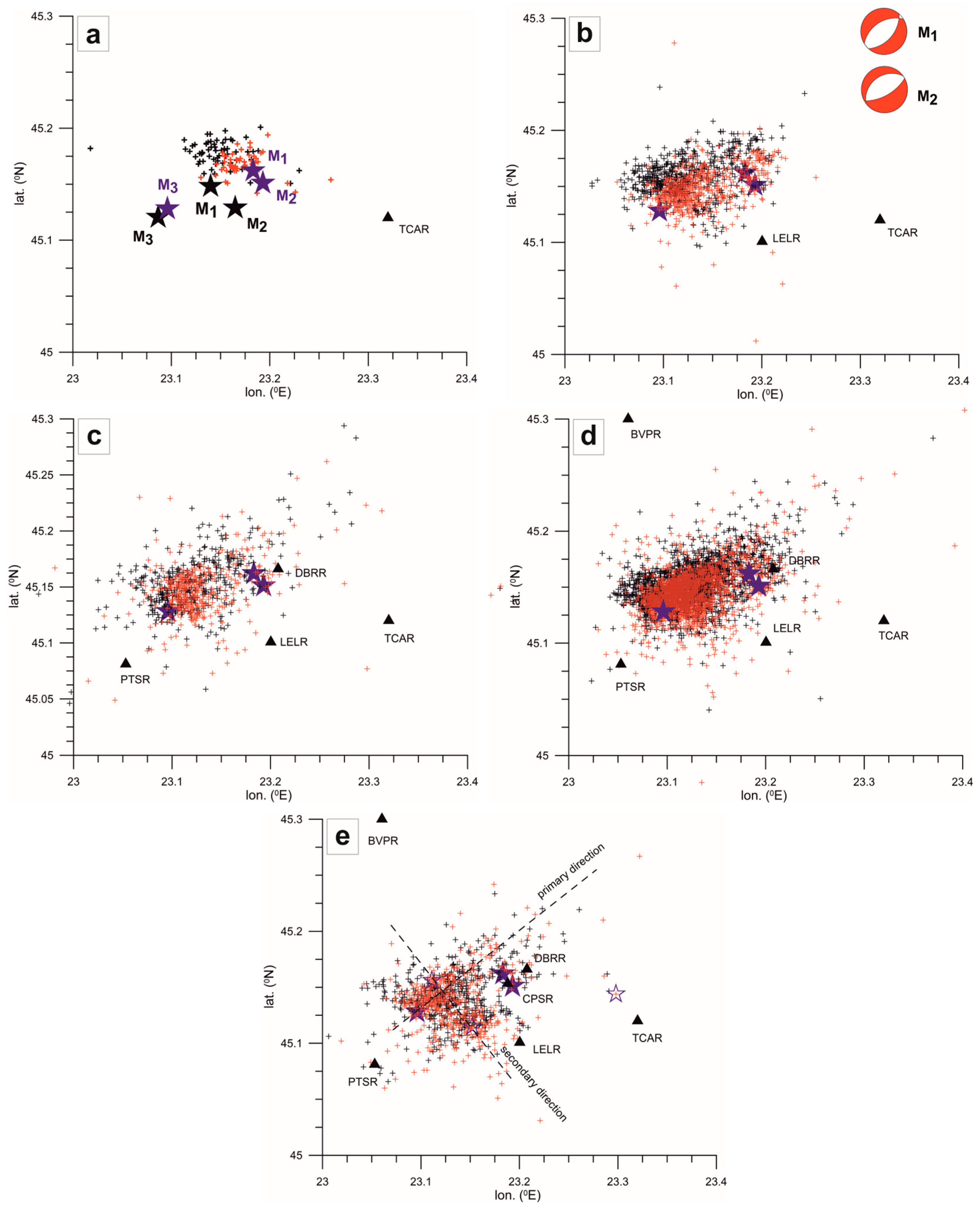
Figure 3.
Histograms of the routinely determined focal depth (a) and with JHD (b). One may note the better constraint of the depth interval and the better stability of depth in the case of JHD locations. As we approach the final stages, the routine locations match better the JHD locations.
Figure 3.
Histograms of the routinely determined focal depth (a) and with JHD (b). One may note the better constraint of the depth interval and the better stability of depth in the case of JHD locations. As we approach the final stages, the routine locations match better the JHD locations.
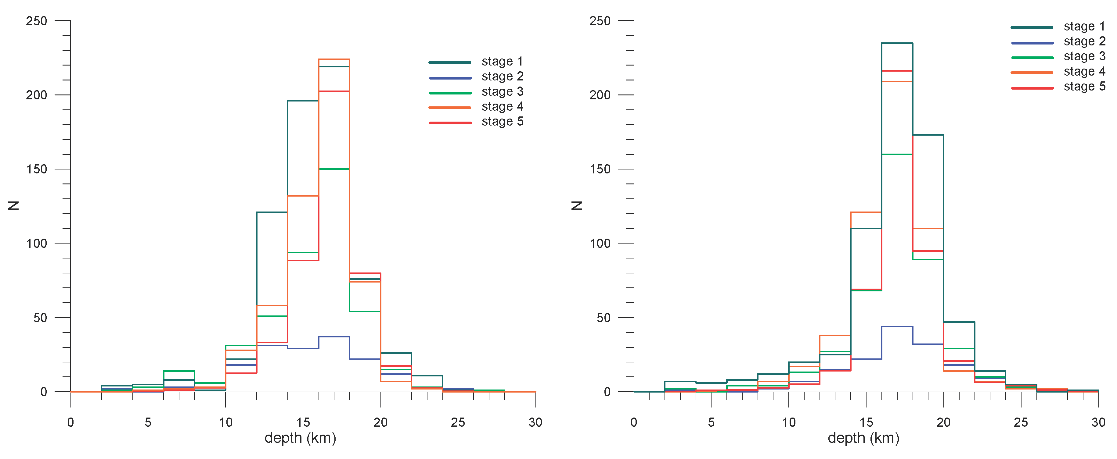
Figure 4.
Histograms of RMS values for routine locations (red line) and JHD locations (blue line) for the events occurred in the five selected time windows corresponding with different stations configurations in the epicentral area.
Figure 4.
Histograms of RMS values for routine locations (red line) and JHD locations (blue line) for the events occurred in the five selected time windows corresponding with different stations configurations in the epicentral area.
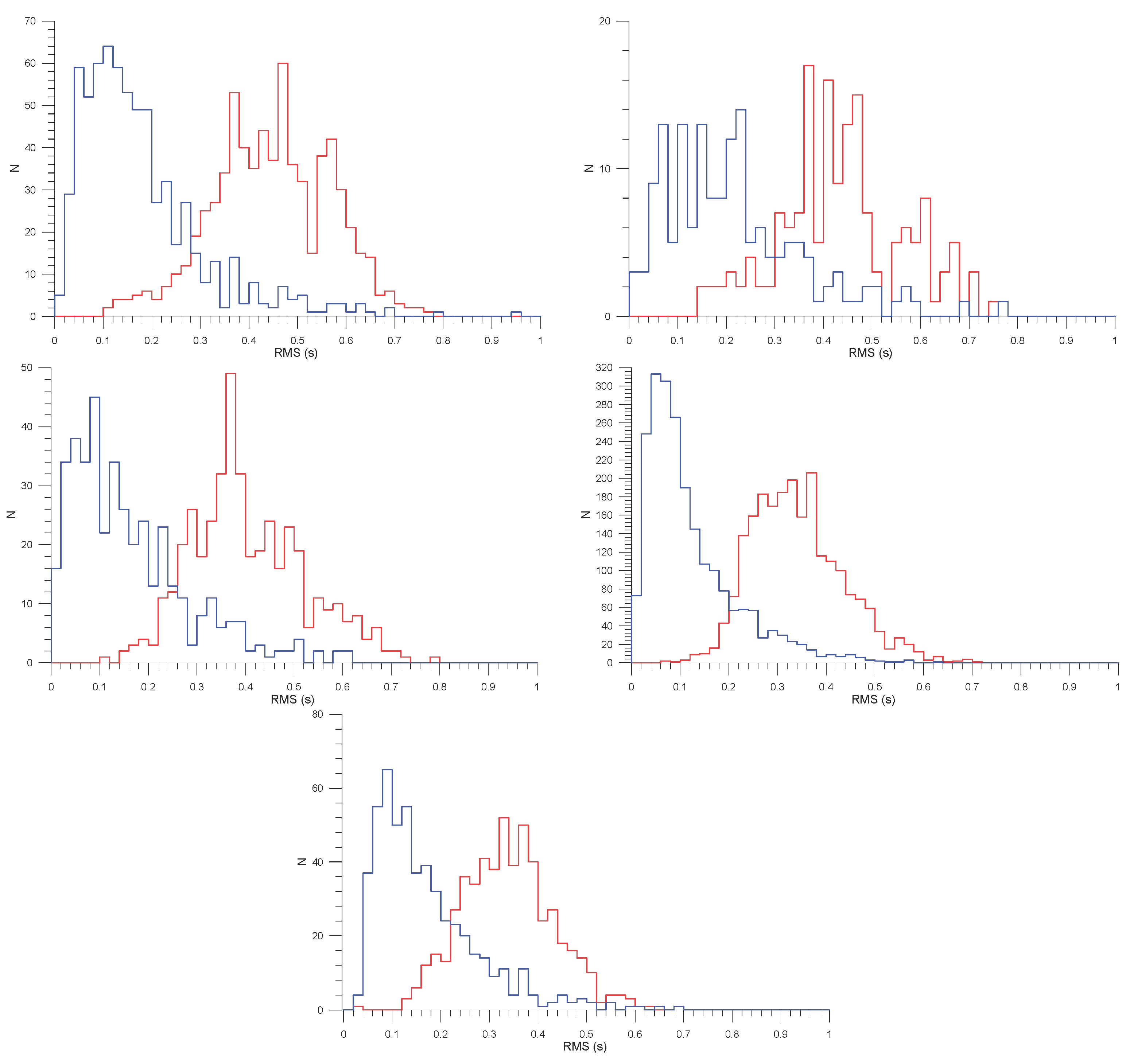
Figure 5.
Seismic activity recorded before the sequence started on 13 February 2023. Stars – epicentres of M1 and M2 events. Diamonds – quarries in the region. Note the increased density of events in the ellipse area where the active quarry of Dobrita is located. It should also be noted the surprising coincidence between M1 and M2 epicentres and the quarry site.
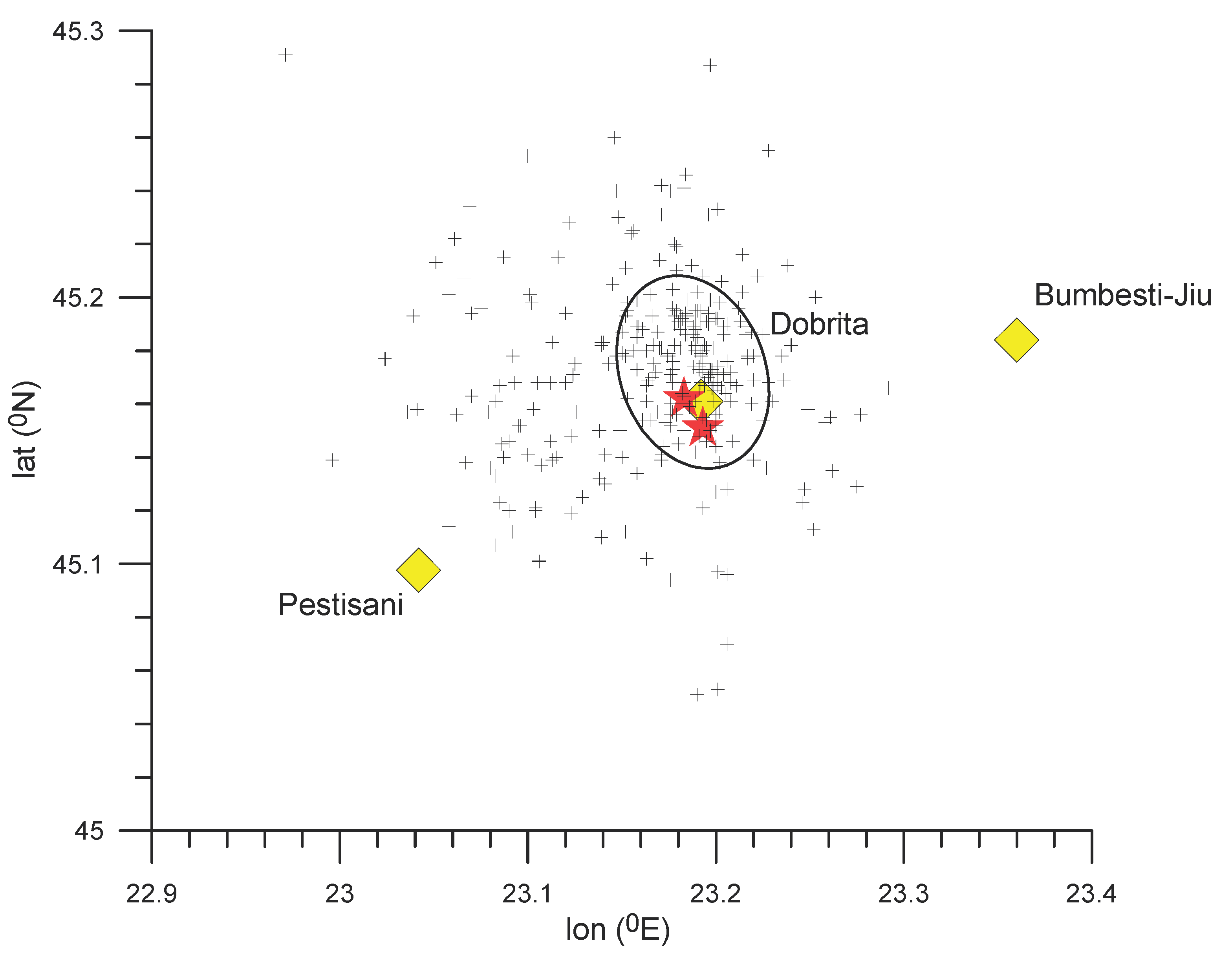
Figure 6.
Day-night distribution of the events before the sequence.
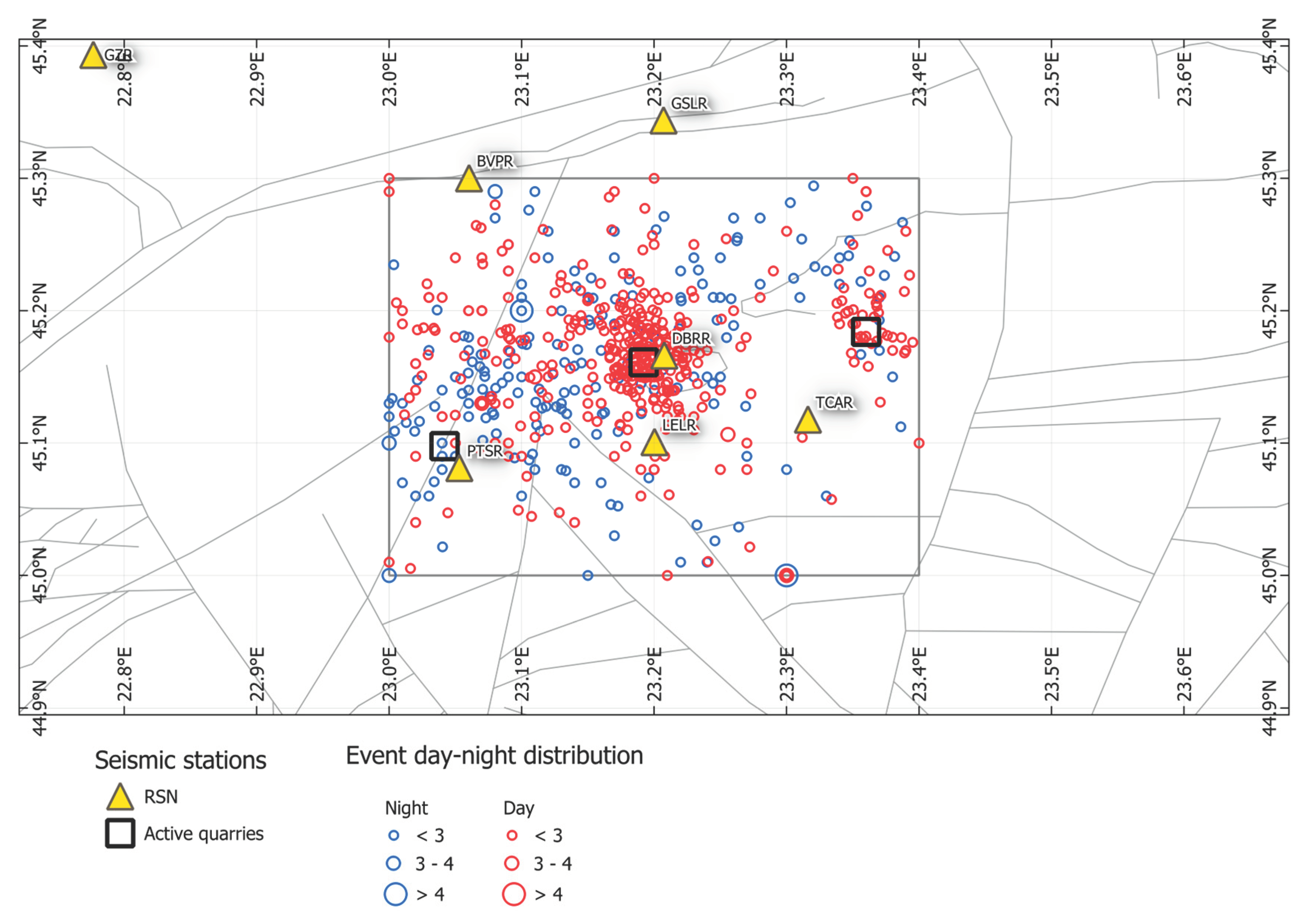
Figure 7.
Wadati diagrams for two sets of events, recorded between 13 February 14:58 and 16 February 07:15 (a), another between 7 July 01:15 and 24 October 19:01 (b). Black symbols: all the stations; red symbols: stations located within 100 km epicentral distance.
Figure 7.
Wadati diagrams for two sets of events, recorded between 13 February 14:58 and 16 February 07:15 (a), another between 7 July 01:15 and 24 October 19:01 (b). Black symbols: all the stations; red symbols: stations located within 100 km epicentral distance.
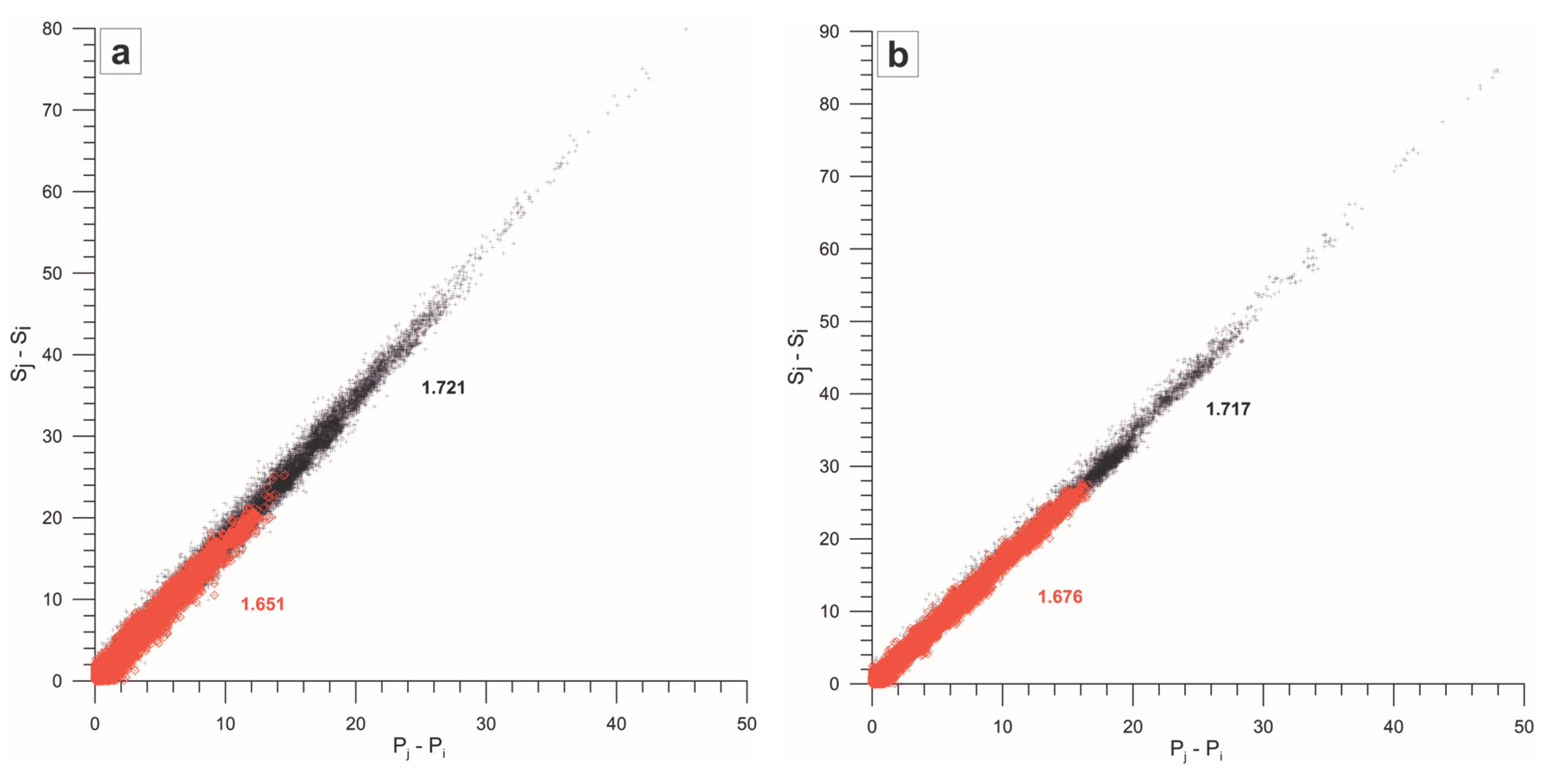
Figure 8.
Evolution in time of the VP/VS ratio. Black symbols: all the stations; red symbols: stations located within 100 km epicentral distance.
Figure 8.
Evolution in time of the VP/VS ratio. Black symbols: all the stations; red symbols: stations located within 100 km epicentral distance.
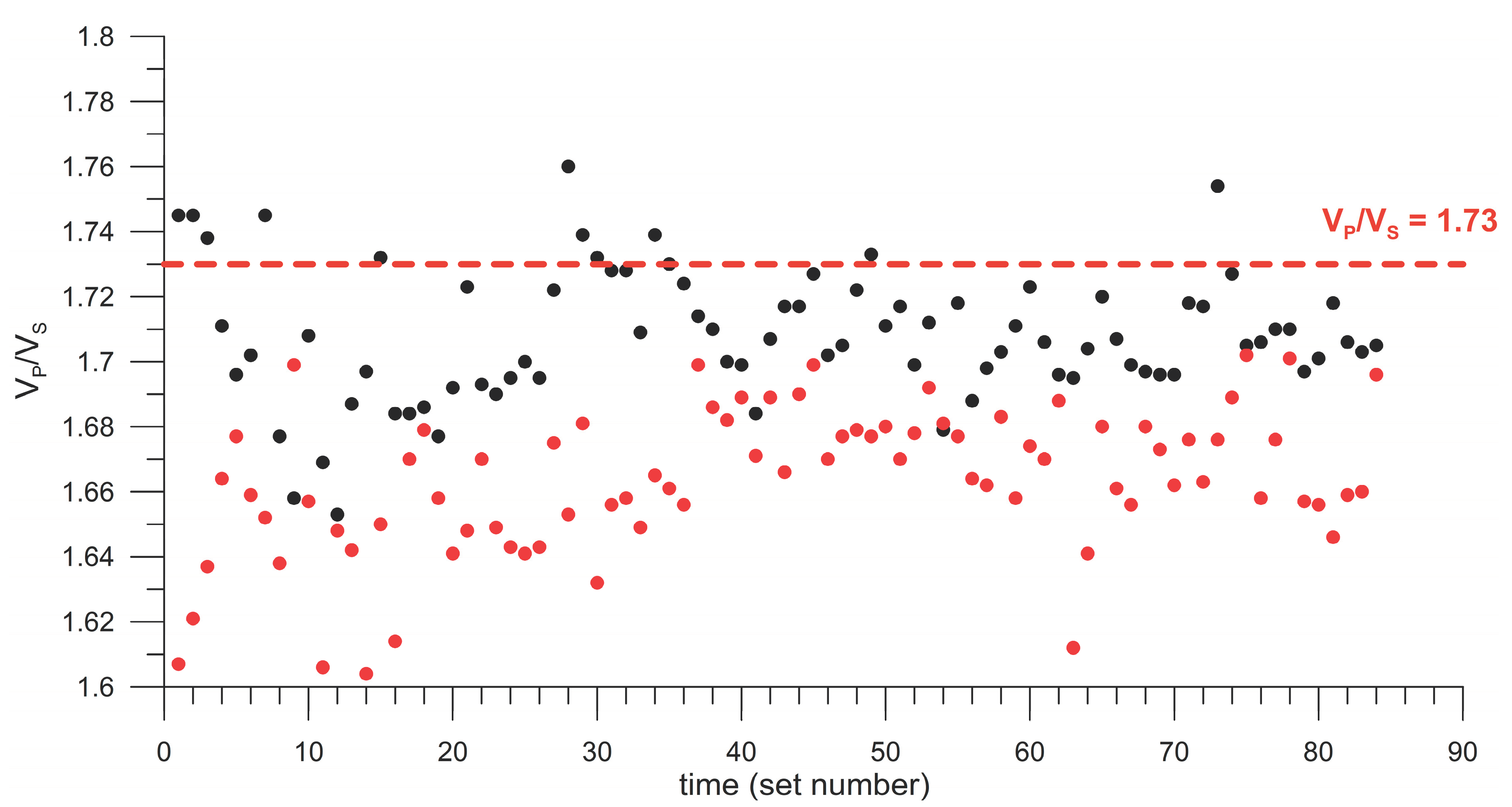

Table 1.
Velocity model used for the JHD technique.
| Depth (km) |
Vp (km/s) |
Vs (km/s) |
|---|---|---|
| 0 | 2.1 | 1 |
| 0.5 | 2.4 | 1.35 |
| 0.5 | 6 | 3.45 |
| 25 | 6.56 | 3.86 |
| 25 | 6.87 | 3.96 |
| 30 | 6.87 | 3.96 |
| 35 | 7.22 | 4.08 |
| 40 | 7.53 | 4.24 |
| 45 | 7.84 | 4.42 |
| 50 | 8.13 | 4.62 |
| 55 | 8.29 | 4.63 |
| 55 | 8.02 | 4.6 |
| 60 | 8.02 | 4.6 |
Disclaimer/Publisher’s Note: The statements, opinions and data contained in all publications are solely those of the individual author(s) and contributor(s) and not of MDPI and/or the editor(s). MDPI and/or the editor(s) disclaim responsibility for any injury to people or property resulting from any ideas, methods, instructions or products referred to in the content. |
© 2024 by the authors. Licensee MDPI, Basel, Switzerland. This article is an open access article distributed under the terms and conditions of the Creative Commons Attribution (CC BY) license (http://creativecommons.org/licenses/by/4.0/).
Copyright: This open access article is published under a Creative Commons CC BY 4.0 license, which permit the free download, distribution, and reuse, provided that the author and preprint are cited in any reuse.


