Submitted:
26 March 2024
Posted:
27 March 2024
You are already at the latest version
Abstract
Keywords:
1. Introduction
2. Data and Methods
2.1. Data
2.1.1. The SBDART Model
2.1.2. ERA5 Reanalysis Data
2.1.3. Satellite Data
- (1)
- FY-4A
- (2)
- CERES
2.2. Research Methods
2.2.1. Algorithm
2.2.2. Evaluation Metrics
- (1)
- The correlation coefficient is used to represent the linear correlation between the predicted values and the actual data and is calculated as follows:
- (2)
- The RMSE represents the error between the retrieved parameter values and the actual data: the smaller the RMSE, the smaller the error between the two values. The RMSE is calculated as follows
- (3)
- The MBE represents the degree to which the parameter values approximate the real data as well as the direction of the deviation between predicted and true values. The MBE is calculated as follows
3. Results
3.1. Sensitivity Analysis Using SBDART
3.1.1. Total Water Vapor Column
3.1.2. Atmospheric Profiles
3.1.3. Surface Temperature
3.2. Validation
3.2.1. Quantitative Verification of
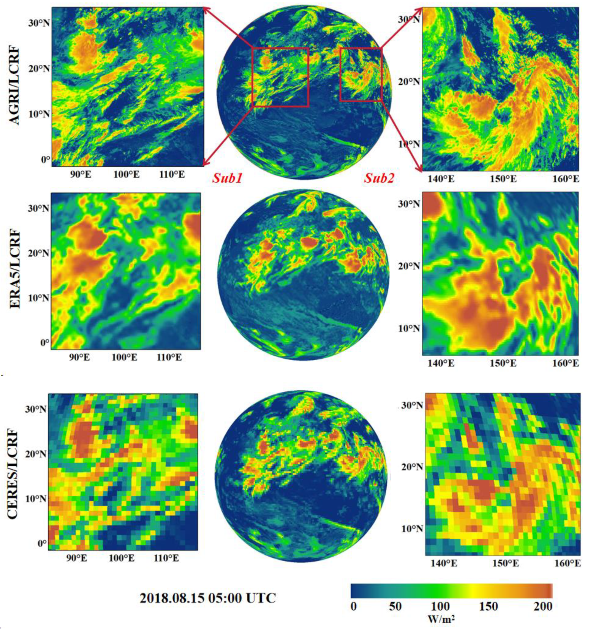
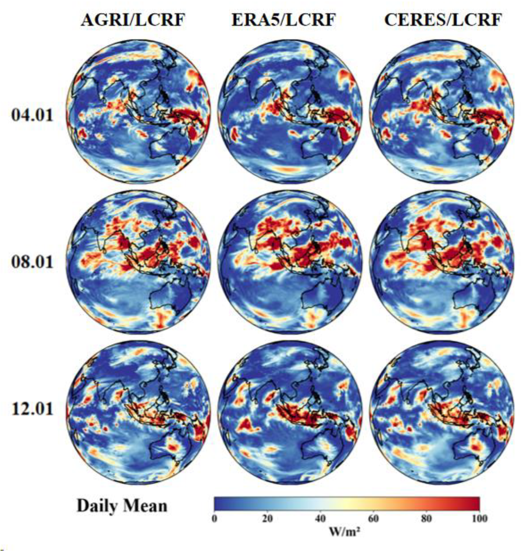
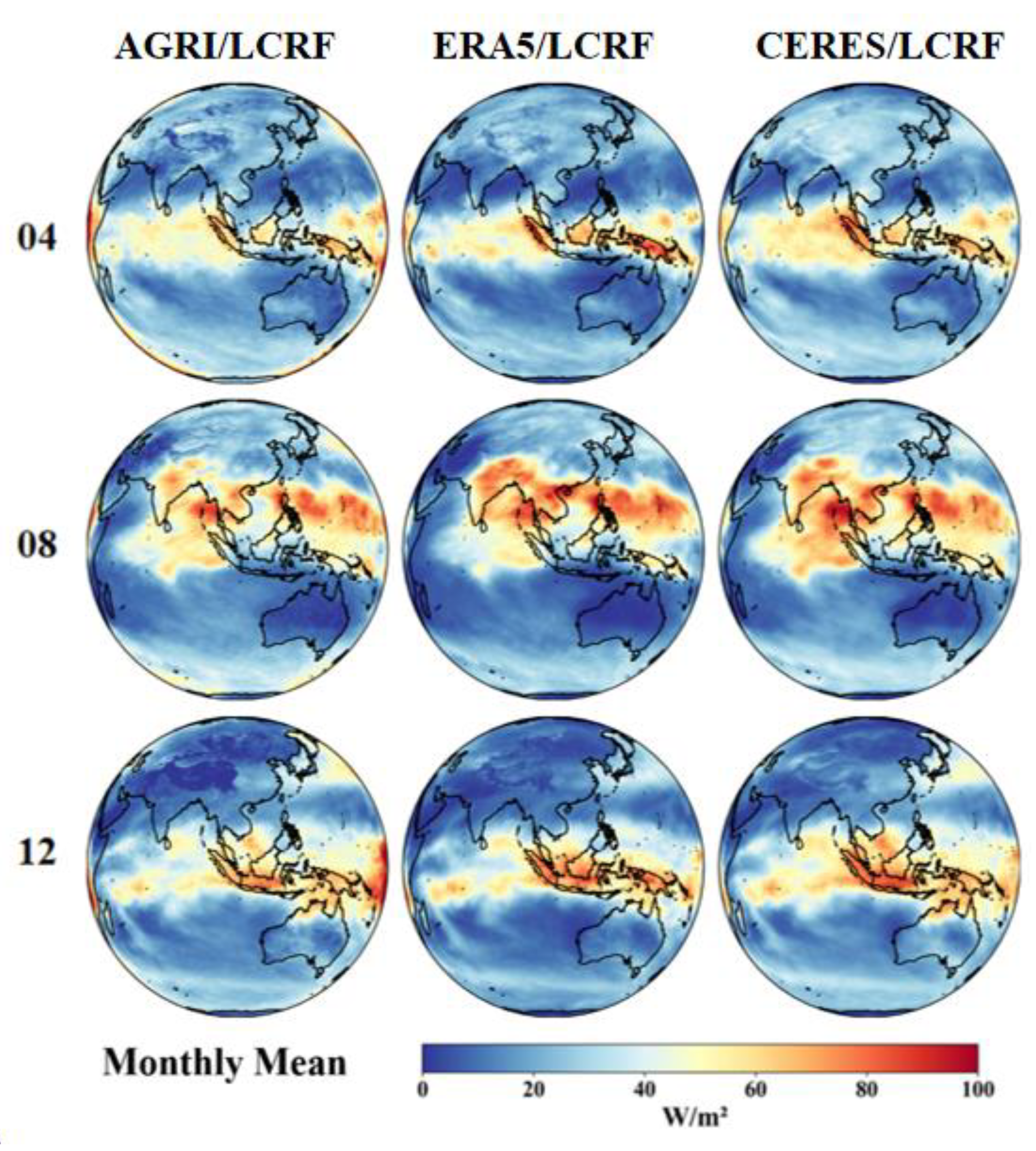
3.2.2. The Spatial Distribution of Results
3.3. Analysis of Changes
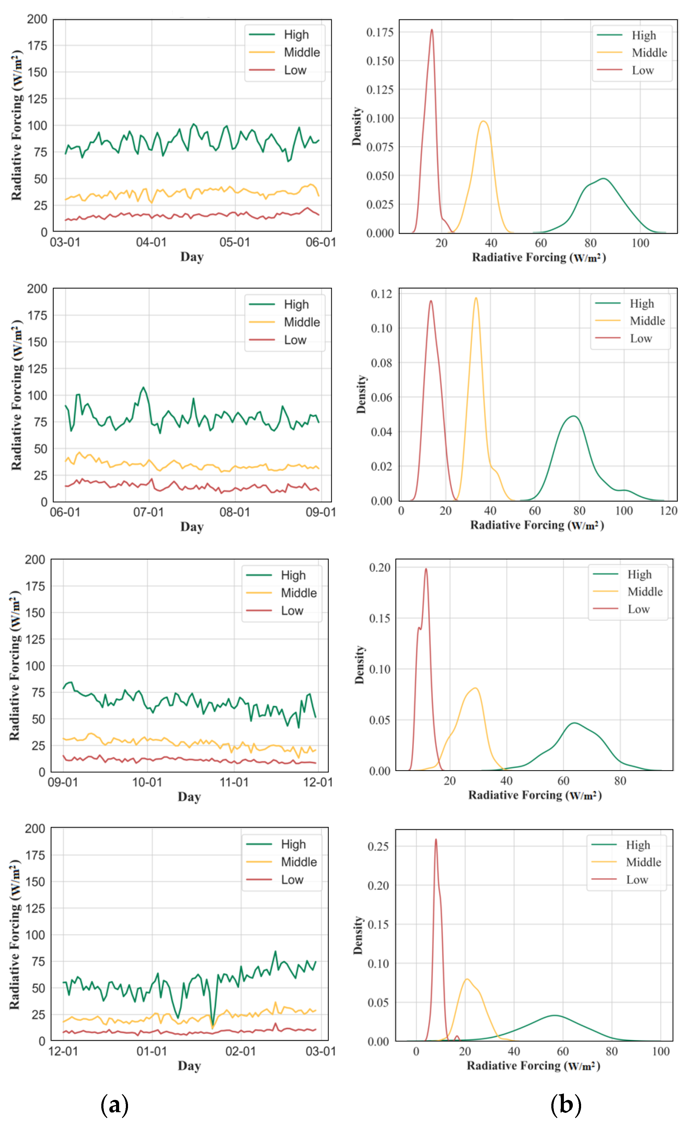
3.3.1. Analysis of Changes due to Varying Clouds Heights
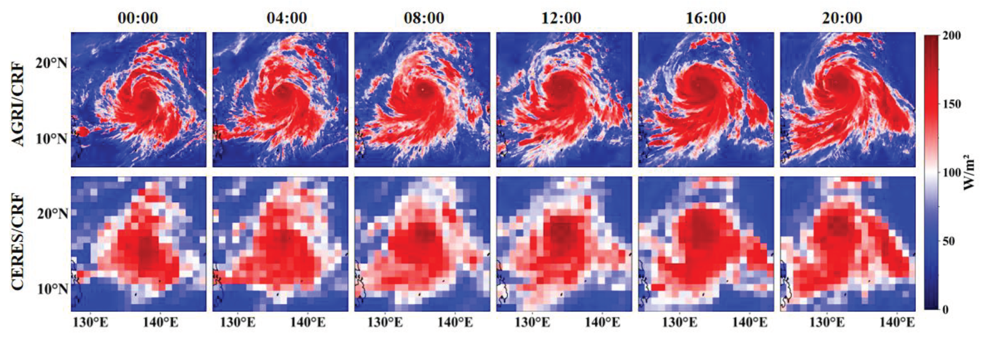
3.3.2. Extreme Event Analysis
4. Discussion and Conclusions
Author Contributions
Funding
Data Availability Statement
Acknowledgments
Conflicts of Interest
References
- Guangyu, S.H.I.; Biao, W.; Hua, Z.; Al, E. The Radiative and Climatic Effects of Atmospheric Aerosols. dqkx 2008, 32, 826–840. [Google Scholar] [CrossRef]
- Karpechko, A.Y.; Manzini, E. Stratospheric Influence on Tropospheric Climate Change in the Northern Hemisphere. J. Geophys. Res. 2012, 117, 2011JD017036. [Google Scholar] [CrossRef]
- Hansen, J.; Sato, M.; Kharecha, P.; von Schuckmann, K. Earth’s Energy Imbalance and Implications. Atmospheric Chemistry and Physics 2011, 11, 13421–13449. [Google Scholar] [CrossRef]
- Intergovernmental Panel On Climate Change Climate Change 2021 – The Physical Science Basis: Working Group I Contribution to the Sixth Assessment Report of the Intergovernmental Panel on Climate Change; 1st ed.; Cambridge University Press, 2023; ISBN 978-1-00-915789-6.
- Tang, W.; Qin, J.; Yang, K.; Liu, S.; Lu, N.; Niu, X. Retrieving High-Resolution Surface Solar Radiation with Cloud Parameters Derived by Combining MODIS and MTSAT Data. Atmospheric Chemistry and Physics 2016, 16, 2543–2557. [Google Scholar] [CrossRef]
- Kato, S.; Rose, F.G.; Rutan, D.A.; Charlock, T.P. Cloud Effects on the Meridional Atmospheric Energy Budget Estimated from Clouds and the Earth’s Radiant Energy System (CERES) Data. Journal of Climate 2008, 21, 4223–4241. [Google Scholar] [CrossRef]
- Kandel, R.; Viollier, M. Observation of the Earth’s Radiation Budget from Space. Comptes Rendus Geoscience 2010, 342, 286–300. [Google Scholar] [CrossRef]
- Wild, M. The Global Energy Balance as Represented in CMIP6 Climate Models. Climate Dynamics 2020, 55, 553–577. [Google Scholar] [CrossRef]
- Wild, M.; Folini, D.; Hakuba, M.Z.; Schär, C.; Seneviratne, S.I.; Kato, S.; Rutan, D.; Ammann, C.; Wood, E.F.; König-Langlo, G. The Energy Balance over Land and Oceans: An Assessment Based on Direct Observations and CMIP5 Climate Models. CLIMATE DYNAMICS 2015, 44, 3393–3429. [Google Scholar] [CrossRef]
- Johnson, G.C.; Lyman, J.M.; Loeb, N.G. Improving Estimates of Earth’s Energy Imbalance. Nature Clim Change 2016, 6, 639–640. [Google Scholar] [CrossRef]
- Zhang, X.; Zhao, X.; Li, W.; Liang, S.; Wang, D.; Liu, Q.; Yao, Y.; Jia, K.; He, T.; Jiang, B.; et al. An Operational Approach for Generating the Global Land Surface Downward Shortwave Radiation Product From MODIS Data. IEEE Trans. Geosci. Remote Sensing 2019, 57, 4636–4650. [Google Scholar] [CrossRef]
- Dedieu, G.; Deschamps, P.Y.; Kerr, Y.H. Satellite Estimation of Solar Irradiance at the Surface of the Earth and of Surface Albedo Using a Physical Model Applied to Metcosat Data. Journal of Applied Meteorology and Climatology 1987, 26, 79–87. [Google Scholar] [CrossRef]
- Liang, S.; Wang, D.; He, T.; Yu, Y. Remote Sensing of Earth’s Energy Budget: Synthesis and Review. International Journal of Digital Earth 2019, 12, 737–780. [Google Scholar] [CrossRef]
- Li, M.; Letu, H.; Peng, Y.; Ishimoto, H.; Lin, Y.; Nakajima, T.Y.; Baran, A.J.; Guo, Z.; Lei, Y.; Shi, J. Investigation of Ice Cloud Modeling Capabilities for the Irregularly Shaped Voronoi Ice Scattering Models in Climate Simulations. Atmospheric Chemistry and Physics 2022, 22, 4809–4825. [Google Scholar] [CrossRef]
- Wang, D.; Liang, S.; Zhang, Y.; Gao, X.; Brown, M.G.L.; Jia, A. A New Set of MODIS Land Products (MCD18): Downward Shortwave Radiation and Photosynthetically Active Radiation. Remote Sensing 2020, 12, 168. [Google Scholar] [CrossRef]
- Letu, H.; Nakajima, T.Y.; Wang, T.; Shang, H.; Ma, R.; Yang, K.; Baran, A.J.; Riedi, J.; Ishimoto, H.; Yoshida, M.; et al. A New Benchmark for Surface Radiation Products over the East Asia–Pacific Region Retrieved from the Himawari-8/AHI Next-Generation Geostationary Satellite. Bulletin of the American Meteorological Society 2022, 103, E873–E888. [Google Scholar] [CrossRef]
- Yu, Y.; Shi, J.; Wang, T.; Letu, H.; Yuan, P.; Zhou, W.; Hu, L. Evaluation of the Himawari-8 Shortwave Downward Radiation (SWDR) Product and Its Comparison With the CERES-SYN, MERRA-2, and ERA-Interim Datasets. IEEE Journal of Selected Topics in Applied Earth Observations and Remote Sensing 2019, 12, 519–532. [Google Scholar] [CrossRef]
- Rutan, D.A.; Kato, S.; Doelling, D.R.; Rose, F.G.; Nguyen, L.T.; Caldwell, T.E.; Loeb, N.G. CERES Synoptic Product: Methodology and Validation of Surface Radiant Flux. Journal of Atmospheric and Oceanic Technology 2015, 32, 1121–1143. [Google Scholar] [CrossRef]
- Barkstrom, B.R. The Earth Radiation Budget Experiment (ERBE). Bulletin of the American Meteorological Society 1984, 65, 1170–1185. [Google Scholar] [CrossRef]
- Liang, S.; Zheng, T.; Liu, R.; Fang, H.; Tsay, S.-C.; Running, S. Estimation of Incident Photosynthetically Active Radiation from Moderate Resolution Imaging Spectrometer Data. Journal of Geophysical Research: Atmospheres 2006, 111. [Google Scholar] [CrossRef]
- Doelling, D.R.; Loeb, N.G.; Keyes, D.F.; Nordeen, M.L.; Morstad, D.; Nguyen, C.; Wielicki, B.A.; Young, D.F.; Sun, M. Geostationary Enhanced Temporal Interpolation for CERES Flux Products. Journal of Atmospheric and Oceanic Technology 2013, 30, 1072–1090. [Google Scholar] [CrossRef]
- Lee, H.-T.; Gruber, A.; Ellingson, R.G.; Laszlo, I. Development of the HIRS Outgoing Longwave Radiation Climate Dataset. Journal of Atmospheric and Oceanic Technology 2007, 24, 2029–2047. [Google Scholar] [CrossRef]
- Park, M.-S.; Ho, C.-H.; Cho, H.; Choi, Y.-S. Retrieval of Outgoing Longwave Radiation from COMS Narrowband Infrared Imagery. Adv. Atmos. Sci. 2015, 32, 375–388. [Google Scholar] [CrossRef]
- Govaerts, Y.M.; Arriaga, A.; Schmetz, J. Operational Vicarious Calibration of the MSG/SEVIRI Solar Channels. Advances in Space Research 2001, 28, 21–30. [Google Scholar] [CrossRef]
- Hou, N.; Zhang, X.; Zhang, W.; Wei, Y.; Jia, K.; Yao, Y.; Jiang, B.; Cheng, J. Estimation of Surface Downward Shortwave Radiation over China from Himawari-8 AHI Data Based on Random Forest. Remote Sensing 2020, 12, 181. [Google Scholar] [CrossRef]
- Ricchiazzi, P.; Yang, S.; Gautier, C.; Sowle, D. SBDART: A Research and Teaching Software Tool for Plane-Parallel Radiative Transfer in the Earth’s Atmosphere. Bulletin of the American Meteorological Society 1998, 79, 2101–2114. [Google Scholar] [CrossRef]
- Kim, B.-Y.; Lee, K.-T.; Jee, J.-B.; Zo, I.-S. Retrieval of Outgoing Longwave Radiation at Top-of-Atmosphere Using Himawari-8 AHI Data. Remote Sensing of Environment 2018, 204, 498–508. [Google Scholar] [CrossRef]
- Hersbach, H.; Bell, B.; Berrisford, P.; Hirahara, S.; Horányi, A.; Muñoz-Sabater, J.; Nicolas, J.; Peubey, C.; Radu, R.; Schepers, D.; et al. The ERA5 Global Reanalysis. Quarterly Journal of the Royal Meteorological Society 2020, 146, 1999–2049. [Google Scholar] [CrossRef]
- Gao, J.; Chen, J.; Tian, X. Ensemble-Learning-Based Cloud Phase Classification Method for FengYun-4 Remote Sensing Images. Infrared Technoiogy 2020, 42, 68–74. [Google Scholar] [CrossRef]
- Smith, G.L.; Priestley, K.J.; Loeb, N.G.; Wielicki, B.A.; Charlock, T.P.; Minnis, P.; Doelling, D.R.; Rutan, D.A. Clouds and Earth Radiant Energy System (CERES), a Review: Past, Present and Future. Advances in Space Research 2011, 48, 254–263. [Google Scholar] [CrossRef]
- Bao, S.; Letu, H.; Zhao, J.; Shang, H.; Lei, Y.; Duan, A.; Chen, B.; Bao, Y.; He, J.; Wang, T.; et al. Spatiotemporal Distributions of Cloud Parameters and Their Response to Meteorological Factors over the Tibetan Plateau during 2003–2015 Based on MODIS Data. International Journal of Climatology 2019, 39, 532–543. [Google Scholar] [CrossRef]
- Ri, X.; Husi, L.; Nakajima, T.Y.; Shi, C.; Gegen, T.; Zhao, J.; Zhang, P.; Chen, L.; Shi, J. Cloud, Atmospheric Radiation and Renewal Energy Application (CARE) Cloud Top Property Product from Himawari-8/AHI: Algorithm Development and Preliminary Validation. 2021, 2021, A14B-08.
- Li, W.; Fang, H. Estimation of Direct, Diffuse, and Total FPARs from Landsat Surface Reflectance Data and Ground-Based Estimates over Six FLUXNET Sites. Journal of Geophysical Research: Biogeosciences 2015, 120, 96–112. [Google Scholar] [CrossRef]

Disclaimer/Publisher’s Note: The statements, opinions and data contained in all publications are solely those of the individual author(s) and contributor(s) and not of MDPI and/or the editor(s). MDPI and/or the editor(s) disclaim responsibility for any injury to people or property resulting from any ideas, methods, instructions or products referred to in the content. |
© 2024 by the authors. Licensee MDPI, Basel, Switzerland. This article is an open access article distributed under the terms and conditions of the Creative Commons Attribution (CC BY) license (http://creativecommons.org/licenses/by/4.0/).


