
Submitted:
19 March 2024
Posted:
20 March 2024
You are already at the latest version
Abstract
Comprehensive understanding of tree characteristics and conditions holds paramount importance for the precise management of hazelnut orchards. It facilitates the determination of tree vigor, pruning requirements, phytosanitary interventions, and plant water consumption. The primary objective of this study was to explore, for the first time on a fruit tree with a bushy structure and across trees of four Italian distinct hazelnut cultivars, the efficacy of multispectral and thermal UAV (Unmanned Aerial Vehicle) technologies in assessing canopy attributes, vegetative growth, and predicting abiotic stresses. These technologies serve as tools for precision agriculture, enabling the computation of various indices such as the Normalized Difference Vegetation Index (NDVI) and crop water stress index (CWSI). The study of water content is of particular importance at this time, especially considering the increasing water stress levels in Europe as well as globally. While Red Green Blue (RGB) and thermal imagery collectively demonstrated superior performance in model reconstruction, the multispectral UAV remained more adept at characterizing size traits of hazelnut plants. Thermal images alone proved inadequate for accurately reconstructing hazelnut biometric characteristics. Furthermore, all indices were found to be cultivar-specific, underscoring the importance of conducting studies across different cultivars. The utilization of two UAVs, namely multispectral and thermal, facilitated the examination of the relationship between NDVI and CWSI across tree species.
Keywords:
CSWI
; Irrigation
; LAI
; NDVI
; Tonda Francescana©
; Tonda Gentile delle Langhe
; Tonda Romana
; Tonda Giffoni
; Water stress
; UAVs
1. Introduction
For a commercial hazelnut orchard, accurate determination of tree size characteristics, such as tree height and canopy volume, holds significant importance for agronomists aiming to assess foliage volume and subsequently enhance agricultural practices including phytosanitary treatments, irrigation, and fertilization [1,2]. This effort promises considerable savings from both economic and environmental perspectives [3,4]. Traditionally managed hazelnut orchards tend to apply irrigation, fertilizers, and other inputs uniformly across all cultivars, disregarding spatial and vigor variations among them [5,6,7]. Hence, to implement optimal site-specific management and enhance environmental sustainability in hazelnut orchards, it’s crucial to identify the spatial variability of soil, crops, and climate, similar to studies conducted for olive orchards [3]. While climate variability, being unmodifiable, is assumed consistent across the orchard, soil variability significantly influences the fertility status of the entire agro-ecosystem [8,9]. Therefore, studying the specific characteristics of each fruit crop based on both climatic requirements and environmental conditions of the study site is advisable.
The structural and biophysical status of each tree in the crop is closely tied to its vigor and can be assessed using various parameters such as TCSA (trunk cross-sectional area), LAI (Leaf Area Index), or canopy volume [8,10]. However, it’s worth noting that canopy measurements and LAI assessment often require non-trivial, highly accurate, and time-consuming techniques, as noted by several researchers [7,11,12]. Consequently, these evaluations are challenging to employ for broad area studies and are often impractical for growers.
Presently, various platforms and sensors are available for evaluating fruit crop variability [13]. Catania et al. [3] delineated three methods for measuring spatial variability in the field: continuous (using sensors on plants or soil), discrete (e.g., point sampling of soil or plant properties), and remote (via aerial or satellite imagery). While discrete sampling offers high precision for the investigated variable, it fails to capture complete variability and necessitates geostatistical techniques for data spatialization. Hence, remote sensing stands out as the most practical data acquisition technique for tree fruit crops in precision agriculture management.
In hazelnut orchards, the preferred platform in recent times is the Unmanned Aerial Vehicle (UAV), equipped with various sensors such as multispectral cameras, which have proven particularly effective in defining tree size characteristics [7,15]. Recent literature [7] presents the evaluation and validation of a straightforward and innovative method for characterizing hazelnut orchard canopies using images captured by UAVs equipped with visible or multispectral cameras.
Recent studies on hazelnuts have highlighted how irrigation management can be enhanced by considering biometric data related to evapotranspiration, such as leaf area and canopy geometry [16,17]. Given that water scarcity increasingly limits crop production, especially in Mediterranean regions where hazelnut orchards are prevalent [8,9], improving irrigation management assumes greater importance.
In tree crops like hazelnuts, assessing plant water status involves various field-level physiological studies such as leaf water potential, stomatal conductance, and net assimilation [6,19]. However, these leaf-level measurements are time-consuming and not easily applicable for operational purposes, particularly when characterizing spatial patterns of physiological processes and plant status variability concerning water stress across the entire orchard. Hence, finding suitable strategies for evaluating within-tree variability of physiological conditions remains challenging, especially for precision agriculture and irrigation management. Recent studies suggest that remote sensing algorithms based on specific parameters directly linked to plant functioning can effectively monitor plant status and water stress in fruit crops [17,18,19].
To devise irrigation strategies effectively, identifying plant water stress indicators and quantifying plant water demand is crucial [17]. Plant water status can be assessed through remote sensing, proximal observations, and spectral analysis techniques, which monitor various indirect parameters linked to it [20]. Infrared thermometers (IRTs) have demonstrated capability in directly tracking crop water stress or computing different stress indices such as the Crop Water Stress Index (CWSI) [21]. CWSI, widely used as an indicator for precision irrigation strategies, is correlated with other stress indicators like leaf water potential and soil water content [22,23,24,25,26]. Quantifying water demand entails evaluating orchard evapotranspiration (ET) under diverse meteorological conditions [8]. Vegetation Indices (VIs) determining crop status on an orchard-wide basis have been closely associated with ET [32]. Regression of NDVI with basal crop coefficients (Kcb) can determine crop water use, as with the FAO 56 method [33,34]. However, within an orchard, spatial differences in soil, canopy structure, and yield affect variations in plant water status, necessitating a plant-based approach over an ET-based one for irrigation management.
Given the recent validation of UAV-acquired measurements compared to field measures [7], the present study aims to explore the potential of multispectral and thermal data from UAV platforms in predicting canopy size characteristics, vegetative growth, and water stress status of trees across four different hazelnut cultivars. This research is essential as orchards typically consist of multiple hazelnut cultivars, given that Corylus avellana L. is a self-sterile species.
2. Materials and Methods
2.1. Study Site Description and Tree Sampling
The research was carried out in the experimental station of the University of Perugia, located in central Italy (42°97′26″N, 12°40′32″E) at 163 m orthometric height, on an irrigated hazelnut (Corylus avellana L.) orchard planted in 2020 with 667 trees ha−1, spaced 4 m between rows and 3.5 m on the row, trained with a single trunk (Figure 1).
The surveys were conducted at the conclusion of summer in 2023 to mitigate potential thermal stress effects resulting from high temperatures. Irrigation of the hazelnut plants [34] was ceased by the end of August. The climatic conditions at the site, from the onset of plant bud break until the time of testing (early October), are depicted in Figures S1 and S2.
Meteorological data were collected using a Spectrum (Thayer Court, Aurora) WatchDog 2000 Series Weather Station situated near the experimental site, with recordings taken at a 15-minute time resolution.
The orchard comprises four Italian hazelnut cultivars: “Tonda Francescana®” (subsequently referred to as T. Francescana or TF), “Tonda Giffoni” (subsequently referred to as T. Giffoni or TG), “Tonda Gentile delle Langhe” (subsequently referred to as T. G. Langhe or TGL), and “Tonda Romana” (subsequently referred to as T. Romana or TR). Sampling was conducted on 24 plants, with six plants selected for each cultivar.
2.2. Manual Measurements
Manual measurements were employed to characterize hazelnut tree canopy parameters such as plant height and canopy volume, following the methodology outlined by [7], where the data obtained through P4M exhibited strong correlation with manual measurements.
The Leaf Area Index (LAI) was determined when the leaf foliage was fully developed, utilizing manual techniques on twenty-four sampled trees. LAI, which denotes the ratio of plant leaf area to canopy cross-sectional area, was calculated by counting the number of leaves at the intersection points of a grid placed within the canopy, with each grid square corresponding to a certain area on the ground. The grid comprised a horizontal bar with holes spaced at 10-centimeter intervals, into which rods were inserted. During measurement, the bar was progressively moved at varying distances from the trunk (e.g., 0 cm, 30 cm, 50 cm, etc.), until no leaves intersected the rods within each hole. The leaves in contact with the rods were counted for each hole and at each distance from the trunk. Furthermore, the leaf area of eight randomly selected leaves from each plant of each variety was determined using a scanner, with pixel values subsequently converted to square centimeters using SigmaScan Pro 5.0 software.
Canopy temperature was assessed using a handheld thermal camera FLIR Ex series #T559828, and the mean temperature within the circular area was computed by measuring the inner part of the canopy (refer to Figure 2) using DJI Thermal Analisys Tool v.3. The difference between canopy temperature and air temperature (ΔT) was compared to thermal UAV data.
2.3. Acquisition of UAV Images
The acquisition was made using a DJI Phantom 4 (P4) Multispectral RTK UAV [41] and a DJI Mavic 3T [42] (Figure 3). To obtain the same Ground Sample Distance (GSD) of about 1.5 cm/pixel, the parameters of the flights were set accordingly.
The P4 RTK multispectral drone (depicted in Figure 3a) is a high-precision aerial platform designed for acquiring multispectral imagery with the positional accuracy of an RTK GNSS receiver. Its imaging system comprises six optics and it’s equipped with ½.9-inch CMOS sensors, including a Red-Green-Blue (RGB) camera (2.08 MPx) and a multispectral sensor covering the blue (B), green (G), red (R), red edge (RE), and near-infrared (NIR) bands. To ensure image accuracy, a spectral sunlight sensor located atop the aircraft detects solar irradiance in real-time. The pitch angle is adjustable within the range of -90° to +30°. The UAV flight planning was conducted using the DJI GSPro app v.2.0.18, employing a polygon grid flight plan with a 10 m altitude, 75% overlap in both side and longitudinal directions, a velocity of 1.5 m/s, and the capture mode “Hover & Capture at Point”. The ground sample distance (GSD) was set to 0.5 cm/pixel. Additionally, the P4 multispectral RTK is equipped with a built-in DJI Onboard D-RTK GNSS receiver, providing centimeter-level positioning accuracy when matched to an RTK station.
The DJI Mavic 3T (depicted in Figure 3b) is equipped with infrared sensing and omnidirectional vision systems. It features two cameras: a ½-inch CMOS sensor capable of capturing 48MP photos with an aperture of f/2.8 and a thermal camera with a resolution of 640x512, supporting point and area measurements. The flight parameters included a 12 m altitude, 75% overlap in both side and heading directions, a velocity of 2 m/s, and a ground sample distance of 0.5 cm/pixel. The Mavic 3T is equipped with an RTK module, ensuring higher accuracy and reliability in positioning by tracking dual-frequency multi-mode signals from visible satellites.
Both the P4 multispectral and Mavic 3T drones were paired with a DJI D-RTK2 GNSS receiver (depicted in Figure 3c), capable of providing centimeter-level accuracy in aircraft positioning during flight. The DJI D-RTK2 receiver supports satellite signal reception from GPS, BEIDU, GLONASS, and Galileo global navigation systems.
2.4. Point Cloud Reconstruction and Maps
The images acquired by P4 Multispetral and Mavic 3T were processed using Agisoft Metashape software (v.1.8.1) [39] to extract the 3D point cloud [7] through the procedure described in [40] (Figure 4). The camera location accuracy was imported to Agisoft Metashape from XMP metadata before processing. The mean error obtained from image processing from P4 Multispectral was 0.058 m, while the mean error obtained from Mavic 3T was 0.054 m. All the images (RGB, RE, NIR) acquired from the P4 Multispectral UAV (follow P4M) were used to obtain the 3D point cloud, the DEM and the orthomosaic (Figure 5a–c respectively) using Metashape. Two distinct projects were conducted utilizing data from the Mavic 3T platform: the initial project employed RGB images (hereafter referred to as M3T) to generate a point cloud (Figure 5d) and a Digital Surface Model (DSM) (Figure 5e). The subsequent project utilized exclusively thermal imagery and the pre-existing DSM (hereafter referred to as M3T_Thermal) to produce a thermal map (Figure 5f). From the Mavic 3T two different projects were done: the first using the RGB images (following reported as M3T) and the second using only thermal images (following reported as M3T_Thermal). The same procedure was applied to obtain the 3D point cloud (Figure 5d), the DSM (Figure 5e) and the orthomosaic (Figure 5f).
The process of extracting canopy information from the 3D point cloud acquired by the P4 Multispectral and Mavic 3T UAVs was conducted as follows:
a) Utilizing the open-source software CloudCompare (v.2.13.alpha), two distinct point clouds—one representing the canopy and the other the ground—were extracted.
b) The point cloud representing the terrain underwent processing to derive the Digital Terrain Model (DTM) using CloudCompare.
c) Within a GIS environment, specifically utilizing the open-source software QGIS (v.3.28.10), the model (ΔH) was generated by computing the pixel-by-pixel difference between the Digital Surface Model (DSM) and the Digital Terrain Model (DTM).
d) The ΔH model was classified into two categories: one for areas where ΔH > 0.2m, representing canopy, and the other for areas where ΔH < 0.2m, representing ground without grass. The 0.2m threshold was chosen to isolate the canopy from ground vegetation.
e) The reclassified ΔH model was vectorized using the “from Raster to Vector” function to produce a shapefile comprising polygons representing each analyzed canopy.
f) The shapefile was augmented with information regarding the different hazelnut cultivars, enabling their visualization on the map.
From the vector model, the canopy area (Ac) was determined, while tree size characteristics (tree height, ht, and canopy height, hc) were computed from the raster data of each tree following the methodology outlined by [6]. Subsequently, these size characteristics were employed to estimate the canopy volume (Vc) using a procedure validated by [6].
The Normalized Difference Vegetation Index (NDVI) was derived from the multispectral orthophoto within a GIS environment using the appropriate formula.
where NIR corresponds to near-infrared digital number and R to red digital number on the same pixel.
As assessed by Kang et al. [41], the LAI-VI relationship could be not unique, particularly in agricultural environment, thus, the values of NDVI described above were used to calculate the Leaf Area Index (LAI) and assess the relationship between NDVI and LAI:
From the elaboration of the thermal images (using Mavic 3T UAV) the orthophoto was obtained and used, in a GIS environment using map algebra functions, to evaluate:
- the thermal map with the formula:
Where Tmeasured represent the temperature registered in the pixel; Gv is the digital number reported in the thermal orthophoto; Tmax and Tmin are the maximum and minimum temperature, respectively; Ngrey is the total number of values that the pixel can be assumed, in this case 8 bit corresponding to 28=256 values;
- the crop water stress index, CWSI, using the formula [19]:
Where Tc= canopy temperature (°C); Ta= air temperature (°C); Tcl= temperature of non-stressed canopy (°C); Tcu= temperature of stressed canopy (°C).
2.5. Statistical Analysis and Evaluation of Model Accuracy
The t-test defines whether the difference between the groups represents a true difference in the study or merely a random difference. The t-test for the comparison of means of different populations (multispectral UAV and thermal UAV) was used to compare the mean size traits (canopy area, Ac, tree height, ht, canopy height, hc and canopy volume V). The test was used to verify the null hypothesis that the difference of the means of size traits and volume obtained from the UAVs (P4M and M3T) is equal to zero. The significant level was set equal to α=0.05.
To validate the measurements of the size traits and canopy volume derived from multispectral UAV (P4M) and thermal UAV (M3T) surveys, a comparison with manual measurements was done and the Pearson correlation coefficient, r, and the root mean square error (RMSE) was calculated. The calculation equation of RMSE is as follows:
where Yi is the sample predicted value (in this case corresponding to UAV data), Xi is the sample actual value (corresponding to manual measurements) and N is the number of samples.
The coefficients of the model (2) were estimated by a least-square linear fit on the variable for each cultivar (considering that LAI is a parameter cultivar-specific [16]) and the related R2 was adopted as a measurement of the corresponding goodness of fit. Moreover, the probability of significant relationship (p-value) was derived and compared to significant level of 5% (α=0.05).
3. Results
3.1. Climatic Condition of the Site and Orchard
The peak heat was recorded during the second decade of July, with the maximum temperature reaching 36.9°C, followed by the third decade of July and the second decade of August, where temperatures exceeded 33°C (refer to Figure S1). Although September remained warm, with maximum temperatures not exceeding 31°C, the mean temperature hovered around 21°C, while the minimum temperature remained around 14°C.
3.2. Comparison of Tree Size Traits and Canopy Volume
In terms of canopy area (Ac) and canopy volume, the t-test indicated that the difference between the mean values obtained from multispectral UAV (P4M) and thermal UAV (M3T) was not statistically significant at α=0.05, yielding values of 2.019 m2 and 2.059 m2, and 1.347 m3 and 1.330 m3, respectively (refer to Table 1).
However, for tree height (ht) and canopy height (hc), the t-test revealed a significant difference (rejecting the null hypothesis) between the means obtained using the multispectral UAV (P4M) and thermal UAV (M3T), resulting in values of 1.922 m and 2.592 m, and 1.340 m and 2.005 m, respectively (refer to Table 1).
To validate the measurements derived from UAV surveys, a comparison with manual measurements was made for each size trait (canopy area, tree height, and canopy height) and canopy volume (Figure 6).
For the canopy area, the comparison between the UAV data, multispectral (P4M) and Mavic 3T (M3T) with manual measurements showed a good agreement with a Pearson coefficient of 0.82, with a RMSE=0.27 m2 and r=0.88 with RMSE=0.25 m2, respectively (Figure 6a,b).
For the tree height, both the comparisons between the multispectral P4M (Figure 7a) and M3T data (Figure 7b) to manual measurements showed a good correlation with r=0.77 and r=0.73, a RMSE=0.40m and RMSE=0.33m respectively.
Also, for the canopy height, the comparisons between the multispectral P4M (Figure 8a) and M3T (Figure 8b) with manual measurements respectively showed a poor correlation with r=0.49 and RMSE=0.38m and r=0.13 and RMSE=0.51m.
For the canopy volume the comparison between the UAV data, multispectral (P4M) and Mavic 3T (M3T) with manual measurements showed a very good agreement with a Pearson coefficient of 0.86, with a RMSE=0.71 m3 and r=0.84 with RMSE=1.34 m3, respectively (Figure 9a,b).
3.3. Estimation of LAI from NDVI Index (Obtained Using the P4M)
NDVI values ranged from –0.96 to 1 (Figure 10a); mean values of NDVI related to the canopies ranged from 0.3836 to 0.5565 (Figure 10b); the lowest value was recorded for T. Romana, equal to 0.453, and the highest value for T. Giffoni (0.528) (Table 2). LAIm (measurements of LAI using obtained with the manual method) varied from 2.211 to 2.77 (Table 2). The lowest value was measured in T. Francescana (2.083) and the highest in T.G. Langhe (2.77) (Table 2).
A multiple correlation analysis showed that the NDVI is not significant to explain the LAI variation (data not shown). In fact, for the same NDVI value, the LAI values of “TGL” and “TG” were very different, while the behavior of “TF” and “TR” resulted more similar (Figure 11). But, the relationship between NDVI and LAI was very significant for cultivar T. Francescana, with R2 equal to 0.7946 and p-value <0.0171; it was quite significant for cultivar T. Romana and T. Giffoni, R2 respectively 0.5812 and 0.6099 per p-value< 0.078 and p-value< 0.0667; it was little significant for cultivar T.G. Langhe with R2 equal to 0.5316 and p-value <0.1002 (Figure 11).
Thermal map obtained from M3T orthophoto (Figure 5f) using Equation (3) showed temperature values between 10.6°C to 49°C (Figure 12a,b).
△T between the canopy temperature, Tc (measured by M3T and using FLIR thermal camera) and air temperature, Ta, resulted to be slightly different (p-value<0.0455), respectively 2.326 °C and 3.175° C; on the contrary, per cultivar, it was different only in T. Giffoni (Table 3).
CWSI values ranged from 0 to 1.575 (Figure 13a); CWSI mean values related to the canopies varied from 0.344 to 0.511 (Figure 13b). In average, the lowest value was measured for T. Romana (0.395) and the highest value for T. Francescana (0.418), (Table 4).
No significant relationship has been found between CWSI obtained from 3MT and LAI from manual measurements (data not shown).
3.4. Comparison between NDVI Index (Obtained Using the P4M) and CWSI Index (Obtained Using the M3T)
The comparison between NDVI and CWSI indices could show a relationship between the chlorophyll content and the water stress of the plant.
This trend is confirmed by the relationship between these two indexes, although it was not very significant and cultivar – dependent (Figure 14). The highest relationships were observed for T. Romana and T. Giffoni cultivar, with R2 equal to 0.5103 and 0.7958 respectively; the lowest relationship was observed for T.G. Langhe (R2 equal to 0.0069) (Figure 14).
4. Discussion
The climatic conditions, particularly the higher temperatures, proved critical for hazelnut plants only during a brief period in July; however, they remained conducive to vegetative and productive growth overall. The mean daily air Vapor Pressure Deficit (VPD) condition from May to August averaged around 1.73 kPa, consistent with findings from other studies on hazelnut [42].
Both the multispectral P4M and thermal M3T UAVs demonstrated effective performance in assessing canopy area (Ac) and canopy volume (V). Notably, there were no significant differences observed between the mean values obtained for Ac and V, and validation with manual measurements exhibited a strong correlation with a Pearson’s coefficient (r > 0.8). Conversely, significant differences were noted for tree height (ht) and canopy height (hc) between the multispectral and thermal UAVs, with low correlations observed with manual measurements. These findings align with previous studies [43] and may be attributed to the obstructed view of the lower portion of the trees by leaves and branches, hindering accurate detection from above.
The multispectral UAV appears to be better suited for evaluating hazelnut orchard size traits. Additionally, the model of canopy points generated by the P4M (approximately 5 million points) is more manageable in terms of processing time and capabilities compared to the model derived from RGB data obtained from the M3T survey (approximately 15 million points).
Both UAVs provide different indices for assessing tree vigor, such as the Normalized Difference Vegetation Index (NDVI), and water stress status, such as the Crop Water Stress Index (CWSI). However, a relationship between NDVI and Leaf Area Index (LAI) was not observed for hazelnut, possibly due to differences in growth habits among cultivars. While some hazelnut cultivars exhibit erect tree growth with a narrow canopy, others have a more expansive canopy, affecting LAI and NDVI values. Nevertheless, moderate relationships between NDVI and LAI were observed for three of the four studied hazelnut cultivars [44].
Regarding canopy temperature, the study found that the mean canopy temperature, extracted from the entire tree using thermal cameras mounted on UAVs, was not easily detected in well-watered orchards. This observation aligns with previous findings in almond trees [26]. Despite this, both survey methods effectively determined the temperature difference (ΔT) between the canopy and air temperature, an important indicator of hazelnut plant abiotic stress [35].
On average, the Crop Water Stress Index (CWSI) recorded for hazelnut trees ranged from 0.344 to 0.511, indicating good water status and stomatal conductance, even after a month without rainfall. Moderate relationships were observed between NDVI and CWSI, with higher NDVI values corresponding to lower CWSI values, consistent with previous studies [47].
5. Conclusions
This study examined the suitability of multispectral and thermal cameras installed on UAVs for measuring the primary growth parameters of fruit trees with bushy structures, specifically focusing on trees of four different hazelnut cultivars varying in vigor and bearing. While both RGB and thermal images exhibited superior performance in model reconstruction, the multispectral UAV proved more adept at estimating hazelnut tree size traits across different cultivars.
This research marks the first example of employing two distinct UAVs to study a bushy tree structure and trees of four different cultivars simultaneously. Typically, studies involve only one type of UAV and examine hazelnut orchards without considering cultivar composition. This approach is crucial for enhancing agricultural practices such as phytosanitary treatments and irrigation, leading to significant economic and environmental benefits.
In conclusion, the study revealed a cultivar-dependent relationship between the Normalized Difference Vegetation Index (NDVI) and Leaf Area Index (LAI) in hazelnut trees, rather than a universal relationship. Furthermore, the survey demonstrated that thermal images alone are insufficient for accurately reconstructing hazelnut canopy shapes. Although thermal cameras on UAVs effectively measure differences between canopy and air temperatures, facilitating the monitoring of abiotic stress, it was noted that higher NDVI values correspond to lower Crop Water Stress Index (CWSI) values. Additionally, CWSI determination requires specific trials of controlled water stress to discern different thresholds.
It is suggested that more discriminatory results may be achieved with older and larger hazelnut trees, and potentially using other digital equipment such as lidar or close-range photogrammetry. Hence, further studies in this direction are warranted.
Supplementary Materials
The following supporting information can be downloaded at the website of this paper posted on Preprints.org, Figure S1: Temperatures (minimum T., Mean T., Maximum T.) and rains at the top; ET0 and vapor pressure deficit at the bottom, recorded from the bud break of plant, in the second decade of March, to the time of test (first decade of October). The data is accompanied by the standard error per decade. Figure S2: Mean and daily radiation.
Author Contributions
Conceptualization, A.V., R.B. and D.F.; methodology, A.V., R.B. and D.F.; software, A.V., V.B. and R.B.; validation, A.V., D.F. and R.B.; formal analysis, A.V. and D.F.; investigation, A.V., R.B., C.T. and D.F.; resources, A.V. and D.F.; data curation, A.V., V.B., C.T., R.B., D.F.; writing—original draft preparation, A.V., R.B. and D.F.; writing—review and editing, A.V.,V.B. and D.F.; visualization, A.V., V.B., R.B. and D.F.; supervision, A.V. and D.F.; project administration, A.V. and D.F.; funding acquisition, A.V. and D.F. All authors have read and agreed to the published version of the manuscript.
Funding
This research received no external funding.
Conflicts of Interest
The authors declare no conflicts of interest.
References
- Carrasco-Benavides M.; Mora M.; Maldonado G.; Olguín-Cáceres J.; von Bennewitz E.; Ortega-Farías S.; Gajardo J.; Fuentes S. Assessment of an automated digital method to estimate leaf area index (LAI) in cherry trees, New Zealand Journal of Crop and Horticultural Science 2016, 44:4, 247–261. [CrossRef]
- Zottele, F.; Crocetta, P.; Baiocchi, V.; How important is UAVs RTK accuracy for the identification of certain vine diseases? 2022 IEEE Workshop on Metrology for Agriculture and Forestry (MetroAgriFor), Perugia, Italy, 2022, pp. 239-243. [CrossRef]
- Catania, P.; Roma, E.; Orlando, S.; Vallone, M. Evaluation of Multispectral Data Acquired from UAV Platform in Olive Orchard. Horticulturae, 2023; 9(2), 133. [CrossRef]
- Miranda-Fuentes, A.; Llorens, J.; Gamarra-Diezma, J.L.; Gil-Ribes, J.A.; Gil, E. Towards an Optimized Method of Olive Tree Crown Volume Measurement. Sensors 2015, 15, 3671–3687. [Google Scholar] [CrossRef] [PubMed]
- Silvestri, C.; Bacchetta, L.; Bellincontro, A.; Cristofori, V. Advances in cultivar choice, hazelnut orchard management, and nut storage to enhance product quality and safety: An overview. J. Sci. Food Agric. 2021, 101, 27–43. [Google Scholar] [CrossRef] [PubMed]
- Portarena, S.; Gavrichkova, O.; Brugnoli, E.; Battistelli, A.; Proietti, S.; Moscatello, S.; Famiani, F.; Tombesi, S.; Zadra, C.; Farinelli, D. Carbon allocation strategies and water uptake in young grafted and own-rooted hazelnut (Corylus avellana L.) cultivars. Tree Physiol. 2022, 42, 939–957. [Google Scholar] [CrossRef] [PubMed]
- Vinci, A.; Brigante, R.; Traini, C.; Farinelli, D. Geometrical Characterization of Hazelnut Trees in an Intensive Orchard by an Unmanned Aerial Vehicle (UAV) for Precision Agriculture Applications. Remote Sens. 2023, 15, 541. [Google Scholar] [CrossRef]
- Vinci, A.; Di Lena, B.; Portarena, S.; Farinelli, D. Trend Analysis of Different Climate Parameters and Watering Requirements for Hazelnut in Central Italy Related to Climate Change. Horticulturae 2023, 9(5), 593. [Google Scholar] [CrossRef]
- FAO, ISPRA & ISTAT A disaggregation of indicator 6.4.2 “Level of water stress: freshwater withdrawal as a proportion of available freshwater resources” at river basin district level in Italy. SDG 6.4 Monitoring Sustainable Use of Water Resources Papers. Rome, FAO. 2023. [CrossRef]
- Caruso, G.; Palai, G.; Marra, F.P.; Caruso, T. High-Resolution UAV Imagery for Field Olive (Olea Europaea L. ) Phenotyping. Horticulturae 2021, 7, 258. [Google Scholar] [CrossRef]
- Grisafi F.; Dejong T.; Tombesi S. Fruit tree crop models: an update. Tree Physiology 2021; 42. [CrossRef]
- Liu, C.; Kang, S.; Li, F.; Li, S.; Du, T. Canopy leaf area index for apple tree using hemispherical photography in arid region. Scientia Horticulturae 2013, 164, 610–615. [Google Scholar] [CrossRef]
- Zhang, C. , Valente, J. , Kooistra, L. et al. Orchard management with small unmanned aerial vehicles: a survey of sensing and analysis approaches. Precision Agric. 2021, 22, 2007–2052. [Google Scholar] [CrossRef]
- Ozdarici A.; Ozgun A. Using remote sensing to identify individual tree species in orchards: A review. Scientia Horticulturae 2023; 321: 112333.
- Roma, E., Catania, P., Vallone, M., & Orlando, S. Unmanned aerial vehicle and proximal sensing of vegetation indices in olive tree (Olea europaea). Journal of Agricultural Engineering, 2023, 54(3).
- Altieri, G.; Maffia, A.; Pastore, V.; Amato, M.; Celano, G. Use of high-resolution multispectral UAVs to calculate projected ground area in Corylus avellana L. tree orchard. Sensors 2022, 22, 7103. [Google Scholar] [CrossRef] [PubMed]
- Vinci, A.; Traini, C.; Portarena, S.; Farinelli, D. Assessment of the Midseason Crop Coefficient for the Evaluation of the Water Demand of Young, Grafted Hazelnut Trees in High-Density Orchards. Water 2023, 15, 1683. [Google Scholar] [CrossRef]
- FAOSTAT. https://www.fao.org/faostat/en/#search/Hazelnuts%2C%20with%20shell (accessed on december 17 2023).
- Camino, C., Zarco-Tejada, P., Gonzalez-Dugo, V. Effects of heterogeneity within tree crowns on airborne-quantified SIF and the CWSI as indicators of water stress in the context of precision agriculture. Remote Sens. 2018, 10, 604. [CrossRef]
- Matese. A.; Baraldi. R.; Berton. A.; Cesaraccio. C.; Di Gennaro. S.; Duce. P.; Facini. O.; Mameli. M.; Piga. A.; Zaldei. A. Estimation of Water Stress in Grapevines Using Proximal and Remote Sensing Methods. Remote Sens. 2018. 10. 114.
- Gardner, B.R., Blad, B.L., Garrity, D.P., Watts, D.G. Relationships between crop temperature, grain yield, evapotranspiration and phenological development in two hybrids of moisture stressed sorghum. Irrig. Sci. 1981, 2 (4), 213–224. [CrossRef]
- Katimbo, A.; Rudnick D., R.; DeJonge, K.C.; Lo, T.H.; Qiao, X.; Franz, T.E.; Nakabuye, H.N.; Duan, J. Crop water stress index computation approaches and their sensitivity to soil water dynamics Agric. Water Manag. 2022, 266, 107575. [Google Scholar] [CrossRef]
- Jackson, R.D., Idso, S.B., Reginato, R.J., Pinter, P.J. Canopy temperature as a crop water stress indicator. Water Resour. Res. 1981, 17 (4), 1133–1138. [CrossRef]
- Jackson, R.D., Kustas, W.P., Choudhury, B.J. A reexamination of the crop water stress index. Irrig. Sci. 1988, 9, 309–317. [CrossRef]
- King, B.A., Shellie, K.C., Tarkalson, D.D., Levin, A.D., Sharma, V., Bjorneberg, D.L. Data-driven models for canopy temperature-based irrigation scheduling. Trans. ASABE 2020, 63 (5), 1579–1592. [CrossRef]
- Gonzalez-Dugo, V., Testi, L., Villalobos, F.J., Lopez-Bernal, ’A., Orgaz, F., Zarco-Tejada, P. J., Fereres, E., 2020. Empirical validation of the relationship between the crop water stress index and relative transpiration in almond trees. Agric. Meteorol. 292–293. [CrossRef]
- Bertalan, L.; Holb, I.; Pataki, A.; Négyesi, G.; Szabó, G.; Szalóki, A.K.; Szabó, S. UAV-based multispectral and thermal cameras to predict soil water content – A machine learning approach, Computers and Electronics in Agriculture 2022, Volume 200, 107262. [CrossRef]
- DeJonge, K.C., Taghvaeian, S., Trout, T.J., Comas, L.H. Comparison of canopy temperature-based water stress indices for maize. Agric. Water Manag. 2015, 156, 51–62. [CrossRef]
- Kullberg, E.G., DeJonge, K.C., Chavez, ´ J.L. Evaluation of thermal remote sensing indices to estimate crop evapotranspiration coefficients. Agric. Water Manag. 2017, 179, 64–73. [CrossRef]
- Kandylakis, Z.; Falagas, A.; Karakizi, C.; Karantzalos, K. Water Stress Estimation in Vineyards from Aerial SWIR and Multispectral UAV Data. Remote Sens. 2020, 12, 2499. [Google Scholar] [CrossRef]
- Z. Han, J. Li, Y. Yuan, X. Fang, B. Zhao, L. Zhu Path recognition of orchard visual navigation based on U-net. Transactions of the Chinese Society for Agricultural Machinery, 52 (1) (2021), pp. 30-39. [CrossRef]
- Glenn, E.P., Neale, C.M.U., Hunsaker, D.J. and Nagler, P.L. Vegetation index-based crop coefficients to estimate evapotranspiration by remote sensing in agricultural and natural ecosystems. Hydrol. Process., 2011, 25: 4050-4062. [CrossRef]
- Bellvert, J.,Adeline, Karine & Baram, Shahar & Pierce, Lars & Sanden, Blake & Smart, David. (2018). Monitoring Crop Evapotranspiration and Crop Coefficients over an Almond and Pistachio Orchard Throughout Remote Sensing. Remote Sensing. 1. 1-22.
- Allen, R.G., Pereira, L.S., Smith, M., Raes, D., Wright, J.L., 2005. FAO-56 dual crop coefficient method for estimating evaporation from soil and application extensions. J. Irrig. Drain. Eng. 131, 2–13.
- Luciani, E., Palliotti, A., Tombesi, S., Gardi, T., Micheli, M., Garcia Berrios, J., Zadra, C., Farinelli, D., Mitigation of multiple summer stresses on hazelnut (Corylus avellana L.): effects of the new arbuscular mycorrhiza Glomus iranicum tenuihypharum sp. nova, Scientia Horticulturae, Volume 257, 2019, 108659. [CrossRef]
- DJI P4 Multispectral User Manual v1.4; 2020. Available online: https://dl.djicdn.com/downloads/p4-multispectral/20190927/P4_Multispectral_User_Manual_v1.0_EN.pdf (accessed on 19 November 2023).
- DJI Mavic 3E_3T User Manual v.1.0; 2022. Available online: https://dl.djicdn.com/downloads/DJI_Mavic_3_Enterprise/DJI_Mavic_3E_3T_User_Manual_EN.pdf (accessed on 19 November 2023).
- DJI D-RTK2 Mobile Station User Manual v.2.0; 2020. Available online: https://dl.djicdn.com/downloads/d-rtk-2/20200611/D-RTK_2_Mobile_Station_User_Guide_v2.0_multi.pdf (accessed on 19 November 2023).
- Agisoft LLC. Agisoft Metashape User Manual, Professional edition, version 1.6; Agisoft LLC: Saint Petersburg, Russia, 2020; 166 p, Available online: https://www.agisoft.com/pdf/ metashape-pro_1_6_en.pdf (accessed on 10 October 2021).
- Vinci, A.; Todisco, F.; Brigante, R.; Mannocchi, F.; Radicioni, F. A smartphone camera for the structure from motion reconstruction for measuring soil surface variations and soil loss due to erosion. Hydrol. Res. 2017, 48, 673–685. [Google Scholar] [CrossRef]
- Kang, Y.; Özdoğan, M.; Zipper, S.C.; Román, M.O.; Walker, J.; Hong, S.Y.; Marshall, M.; Magliulo, V.; Moreno, J.; Alonso, L.; et al. How Universal Is the Relationship between Remotely Sensed Vegetation Indices and Crop Leaf Area Index? A Global Assessment. Remote Sens. 2016, 8, 597. [Google Scholar] [CrossRef] [PubMed]
- Pasqualotto G., Carraro V., Suarez Huerta E. and Anfodillo T. Assessment of Canopy Conductance Responses to Vapor Pressure Deficit in Eight Hazelnut Orchards Across Continents. Front. Plant Sci. 2021, 12:767916. [CrossRef]
- Patrick, A.; Li, C. High Throughput Phenotyping of Blueberry Bush Morphological Traits Using Unmanned Aerial Systems. Remote Sens. 2017, 9, 1250. [Google Scholar] [CrossRef]
- Bioversity, FAO and CIHEAM. 2008. Descriptors for hazelnut (Corylus avellana L.). Bioversity International, Rome, Italy; Food and Agriculture Organization of the United Nations, Rome, Italy; International Centre for Advanced Mediterranean Agronomic Studies, Zaragoza, Spain. ISBN: 978-92-9043-762-8 (https://qrgj.org/wp-content/uploads/2022/01/Descriptors-for-hazelnut-Corylus-avellana-L..pdf).
- Bignami, C.; Natali, S. Influence of irrigation on the growth and production of young hazelnuts. Acta Hort. 1997. [CrossRef]
- Tombesi, A., Rosati, A.. Hazelnut response to water levels in relation to productive cycle. In IV International Symposium on Hazelnut (1996, July) 445 (pp. 269-278).
- Dong-Ho, L., Park, J.-H., Comparison between NDVI and CWSI for waxy corn growth monitoring in field soil conditions. Remote Sensing for Agriculture, Ecosystems, and Hydrology XXI. 2019 Vol. 11149.
Figure 1.
Experimental station’s photo where the red rectangle indicates the hazelnut orchard in the study.
Figure 1.
Experimental station’s photo where the red rectangle indicates the hazelnut orchard in the study.
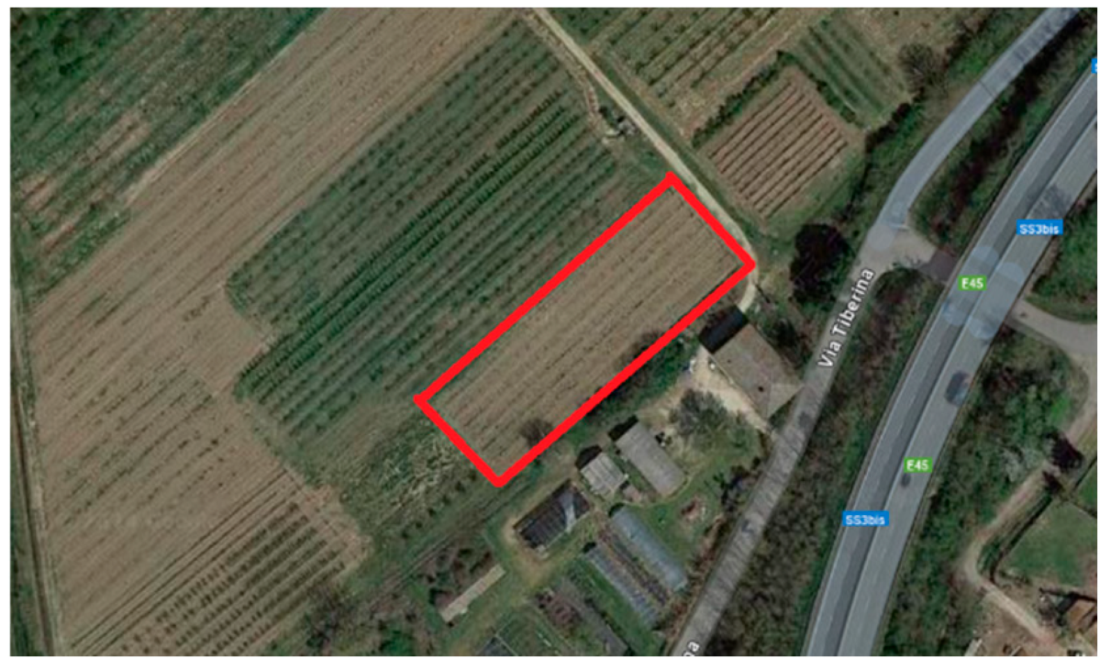
Figure 2.
Thermal Image (a); Thermal image and photo overlap (b); Measured temperature of the canopy and thermal camera information (c).
Figure 2.
Thermal Image (a); Thermal image and photo overlap (b); Measured temperature of the canopy and thermal camera information (c).
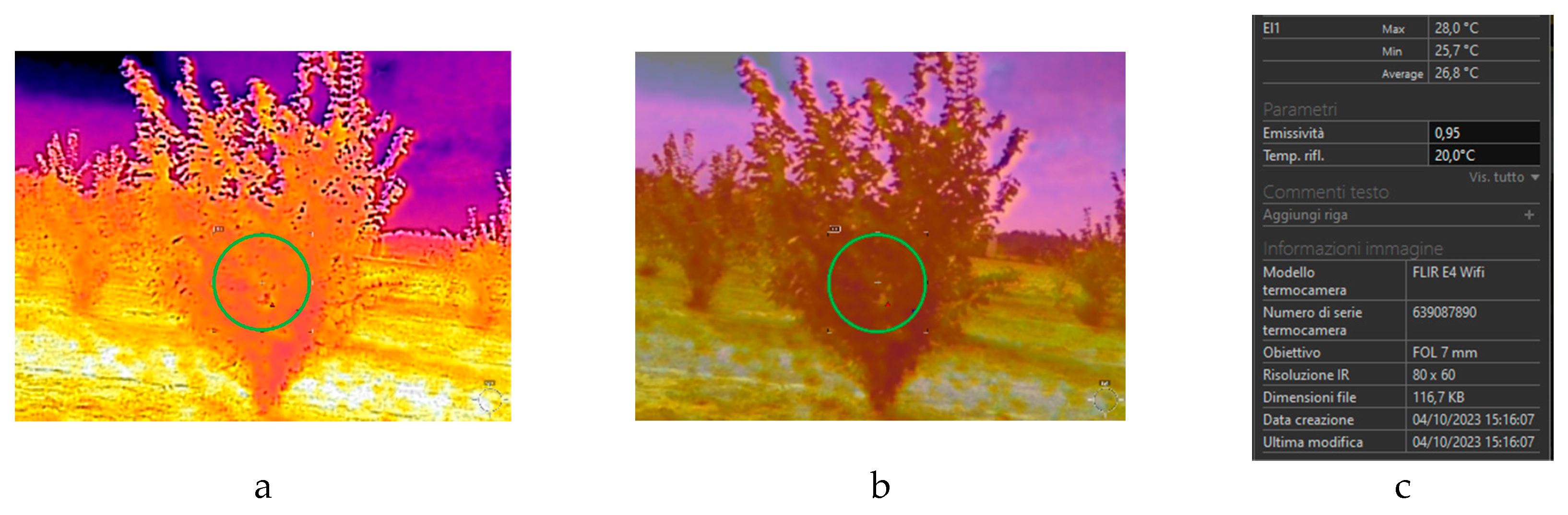
Figure 3.
DJI Phantom 4 RTK Multispectral (a); DJI Mavic 3T (b); DJI D-RTK2 mobile station (c).
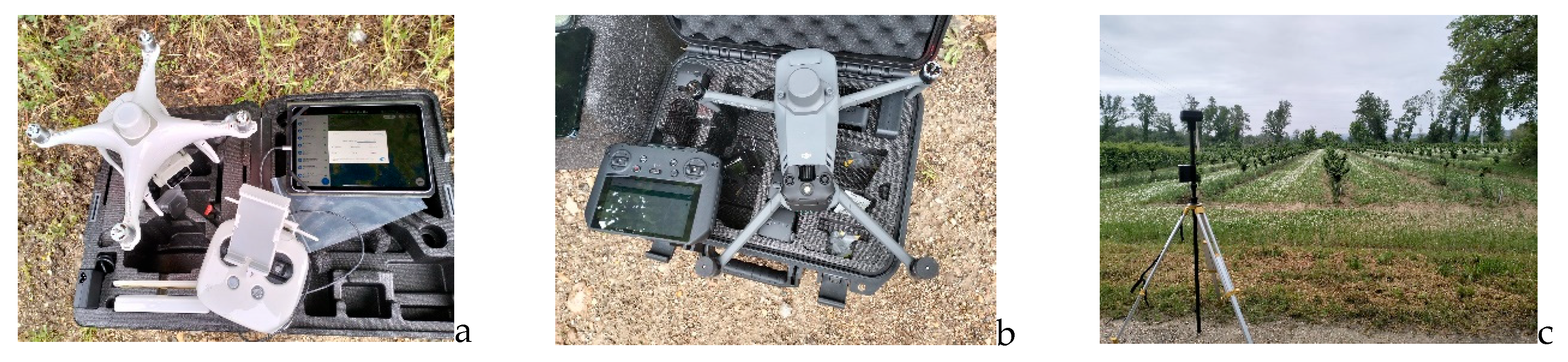
Figure 4.
Flowchart of the procedure used to obtain the Multispectral and Thermal maps.
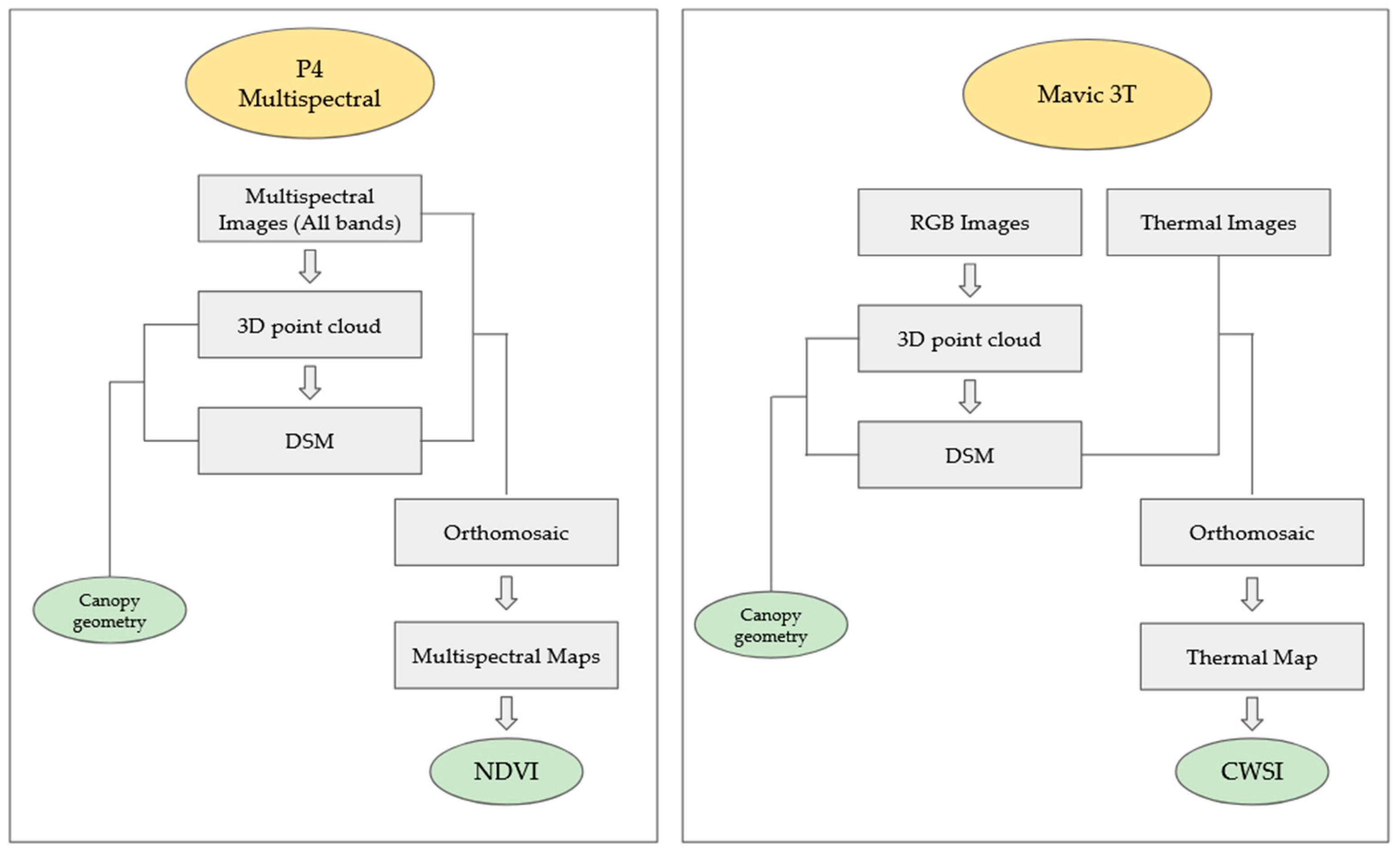
Figure 5.
Elaboration output of the P4M images: 3D point cloud (a), DSM (b), orthomosaic (c); Elaboration output of the M3T RGB and thermal images: 3D point cloud (d), DSM (e), orthomosaic (f).
Figure 5.
Elaboration output of the P4M images: 3D point cloud (a), DSM (b), orthomosaic (c); Elaboration output of the M3T RGB and thermal images: 3D point cloud (d), DSM (e), orthomosaic (f).
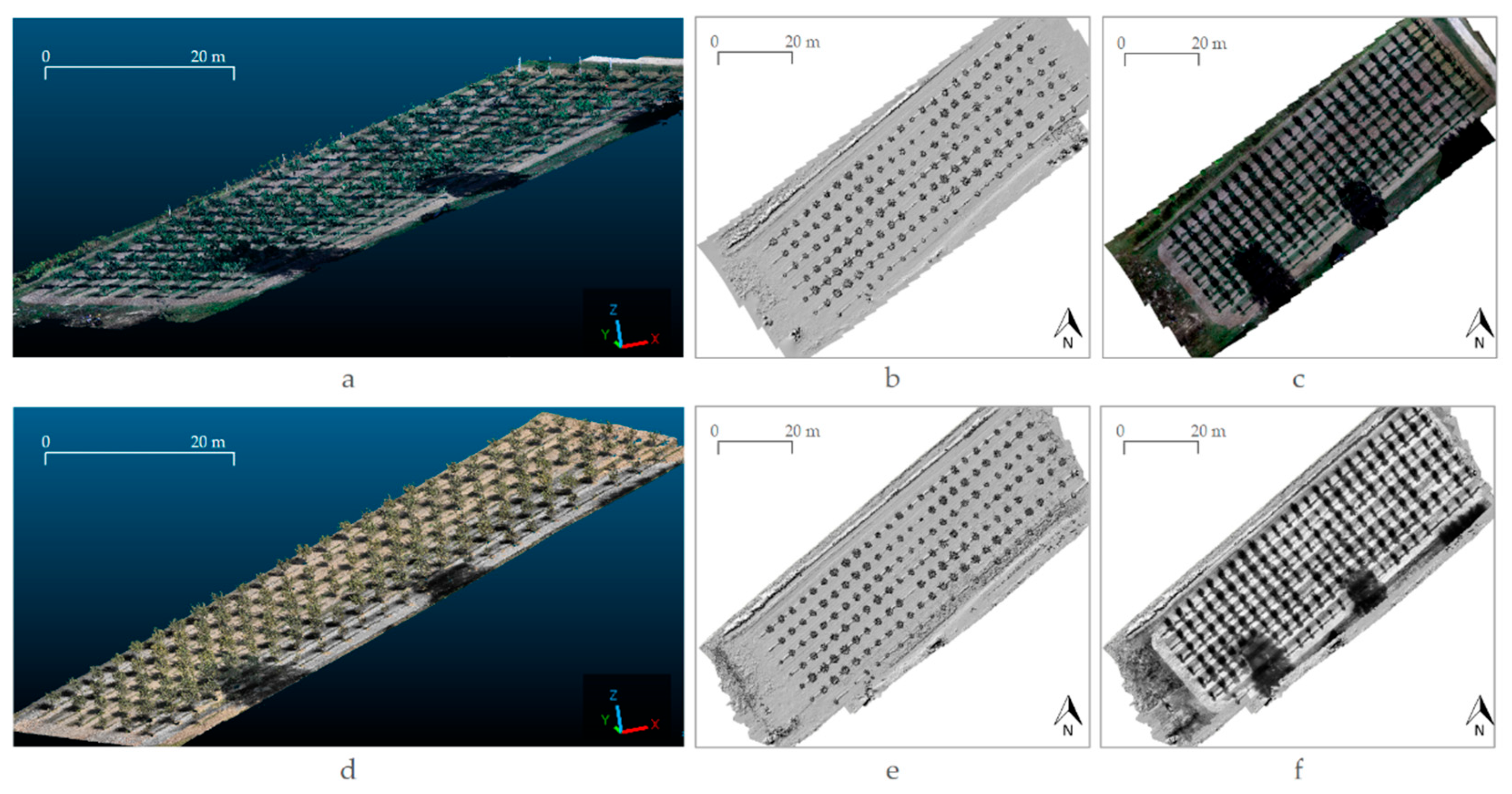
Figure 6.
Canopy area comparison between multispectral UAV (P4M) data and manual measurements (a) and thermal UAV (M3T) and manual measurements (b). Red line represents 1:1.
Figure 6.
Canopy area comparison between multispectral UAV (P4M) data and manual measurements (a) and thermal UAV (M3T) and manual measurements (b). Red line represents 1:1.
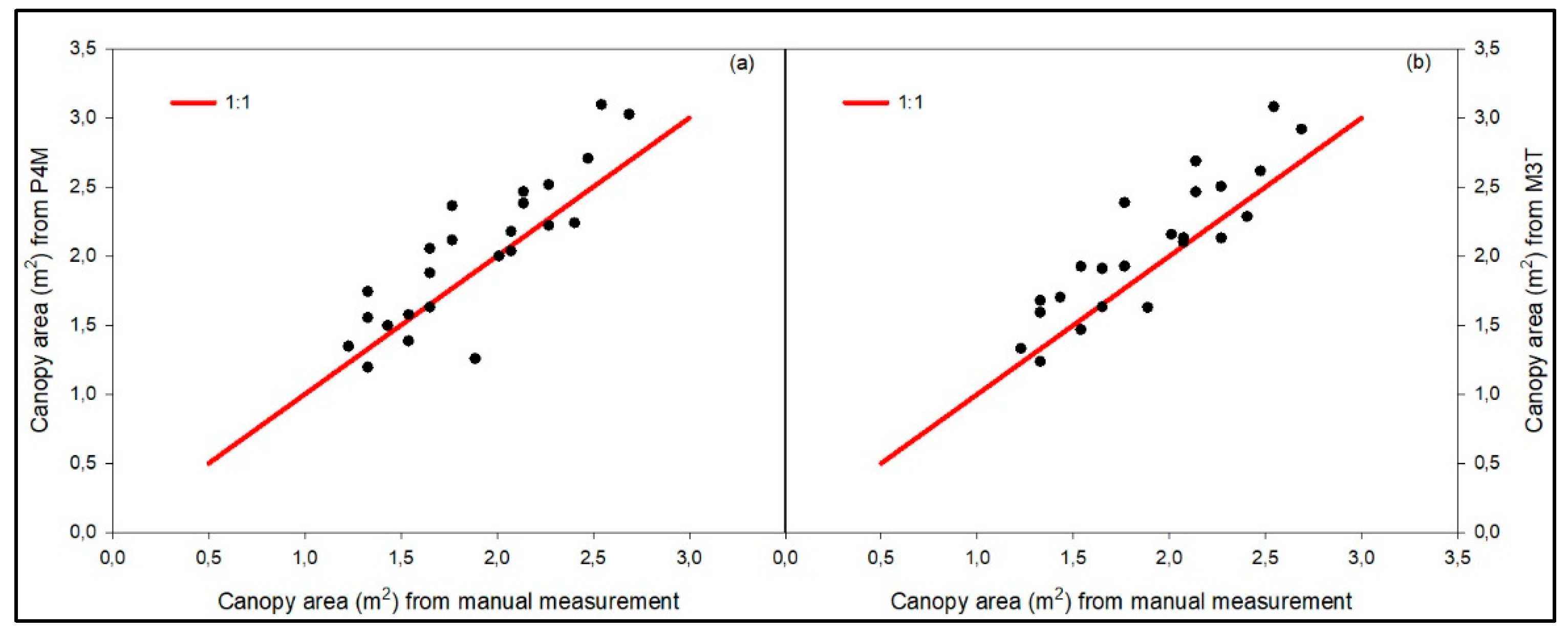
Figure 7.
Tree height comparison between multispectral UAV (P4M) data and manual measurements (a) and thermal UAV (M3T) and manual measurements (b). Red line represents 1:1.
Figure 7.
Tree height comparison between multispectral UAV (P4M) data and manual measurements (a) and thermal UAV (M3T) and manual measurements (b). Red line represents 1:1.
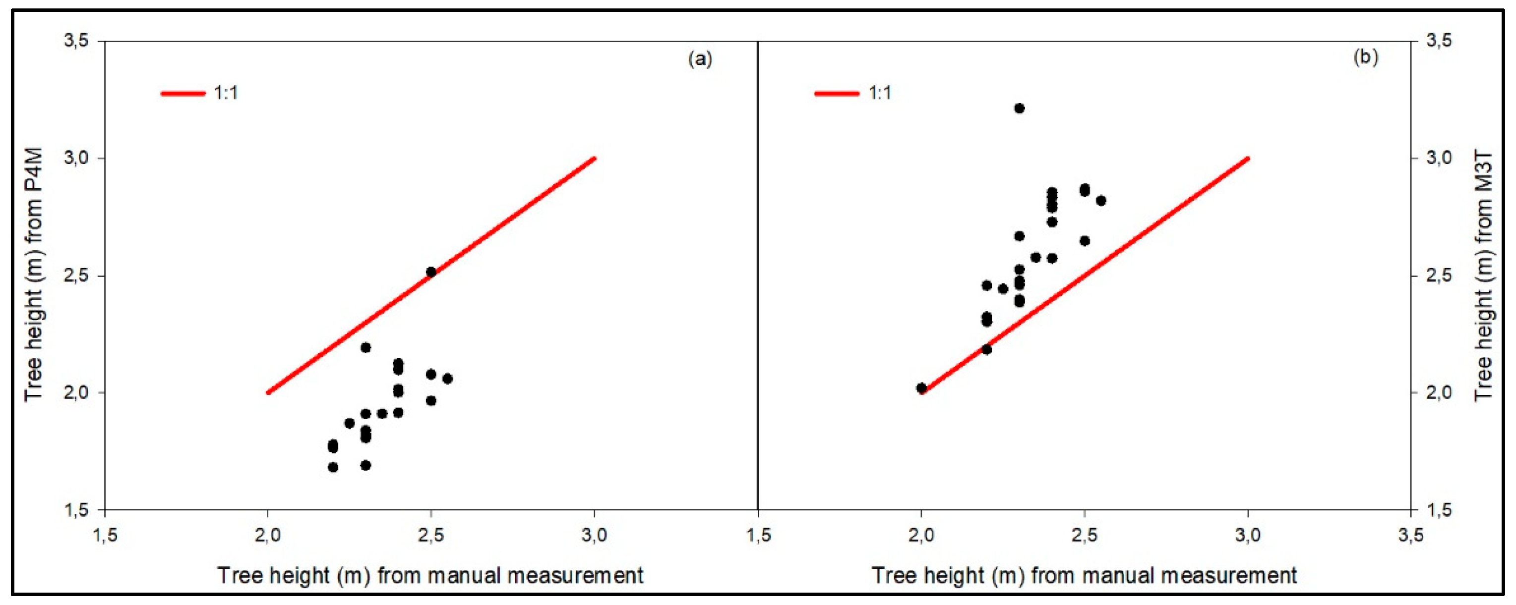
Figure 8.
Canopy height comparison between multispectral UAV (P4M) data and manual measurements (a) and thermal UAV (M3T) and manual measurements (b). Red line represents 1:1.
Figure 8.
Canopy height comparison between multispectral UAV (P4M) data and manual measurements (a) and thermal UAV (M3T) and manual measurements (b). Red line represents 1:1.
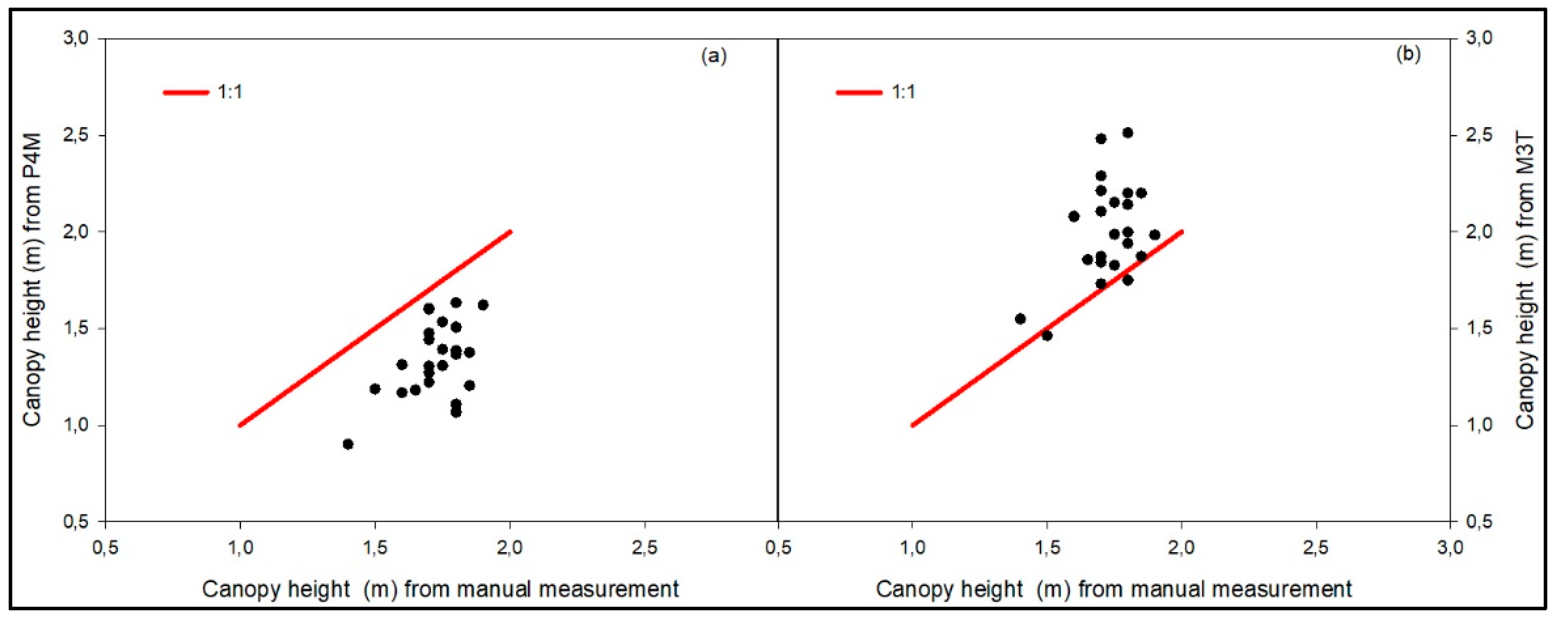
Figure 9.
Canopy volume comparison between multispectral UAV (P4M) data and manual measurements (a) and thermal UAV (M3T) and manual measurements (b). Red line represents 1:1.
Figure 9.
Canopy volume comparison between multispectral UAV (P4M) data and manual measurements (a) and thermal UAV (M3T) and manual measurements (b). Red line represents 1:1.
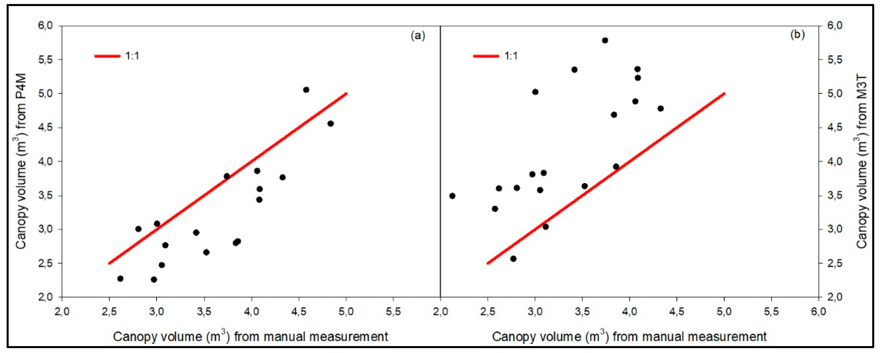
Figure 10.
NDVI maps: index values related to the canopy (a) and mean values related to the investigated trees (b).
Figure 10.
NDVI maps: index values related to the canopy (a) and mean values related to the investigated trees (b).
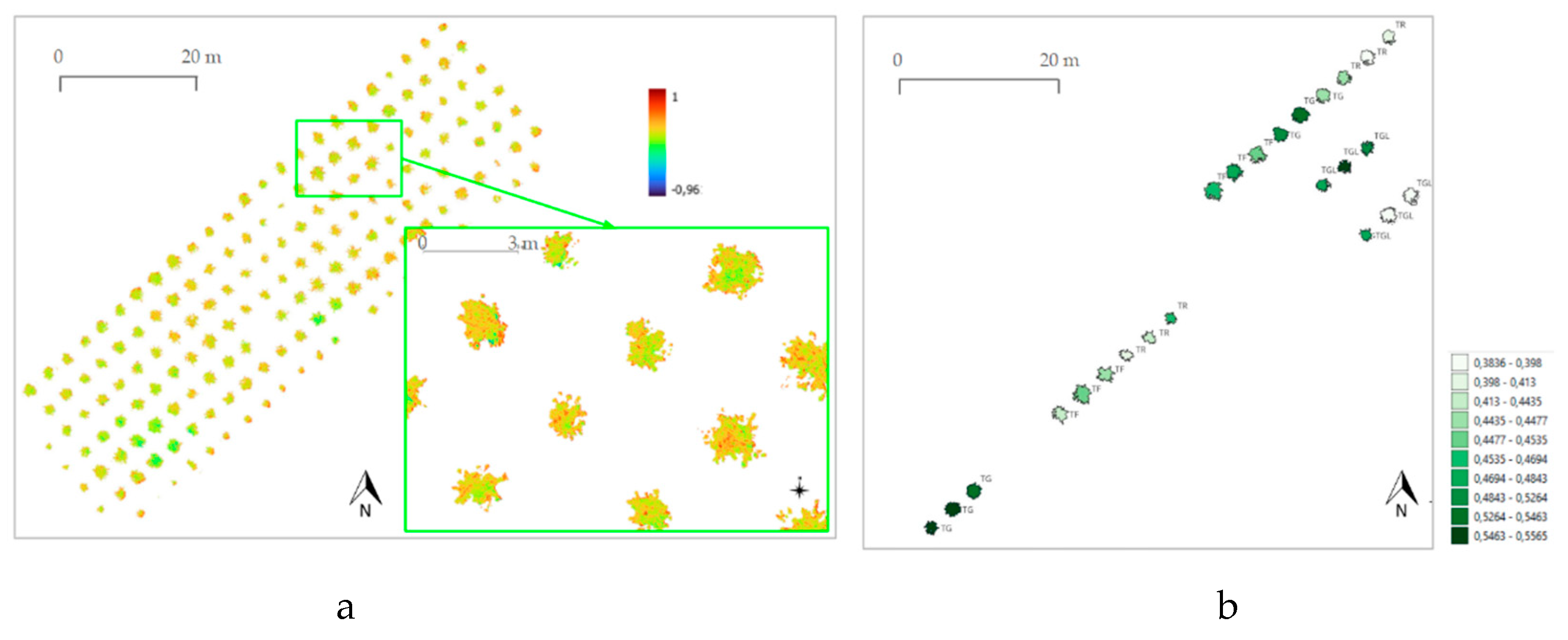
Figure 11.
Relationship between NDVI mean obtained from P4M and LAI per each cultivar.
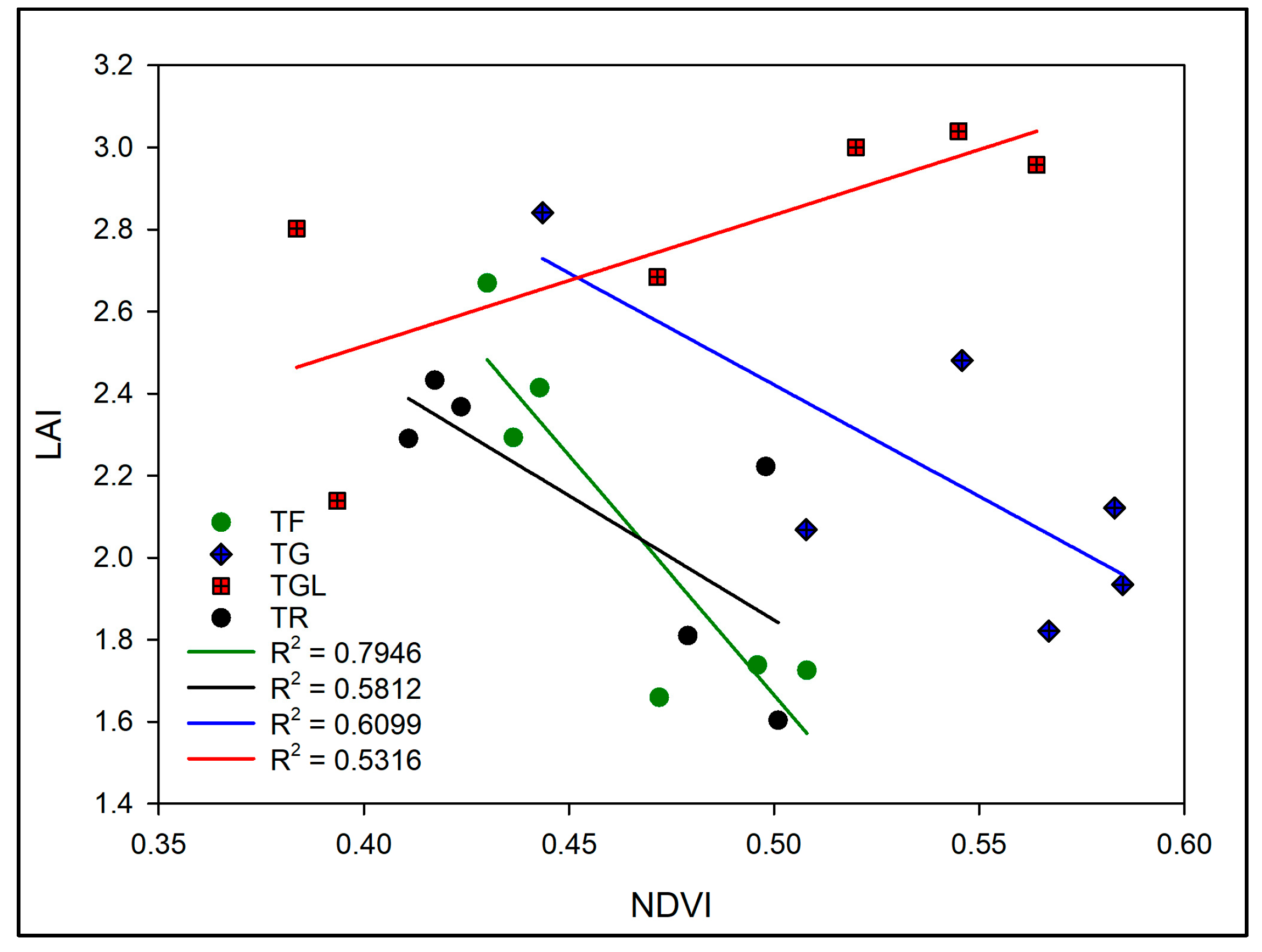
Figure 12.
Thermal map: temperature values obtained from Equation (3) (a) and temperature values of the canopies (b).
Figure 12.
Thermal map: temperature values obtained from Equation (3) (a) and temperature values of the canopies (b).
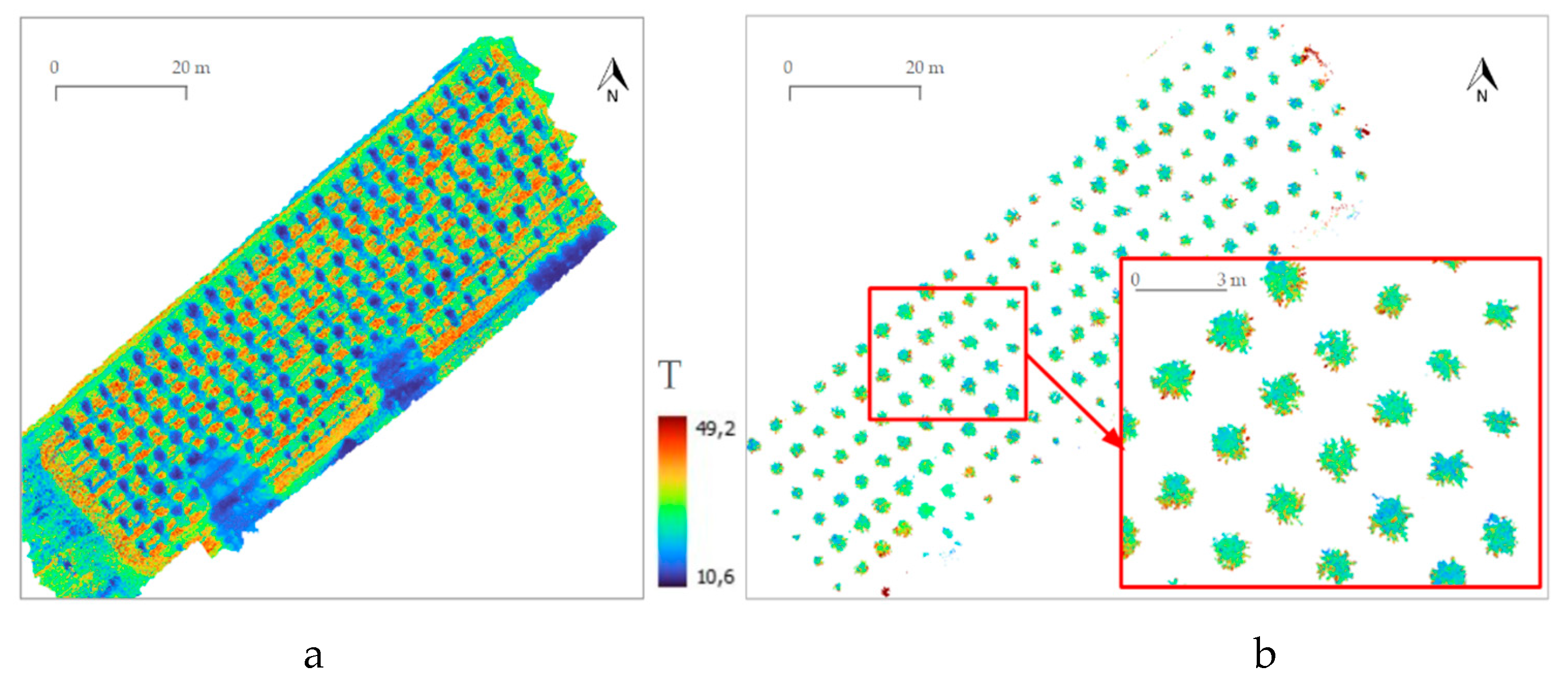
Figure 13.
CWSI maps: index values related to the canopy (a) and mean values related to the investigated trees (b).
Figure 13.
CWSI maps: index values related to the canopy (a) and mean values related to the investigated trees (b).
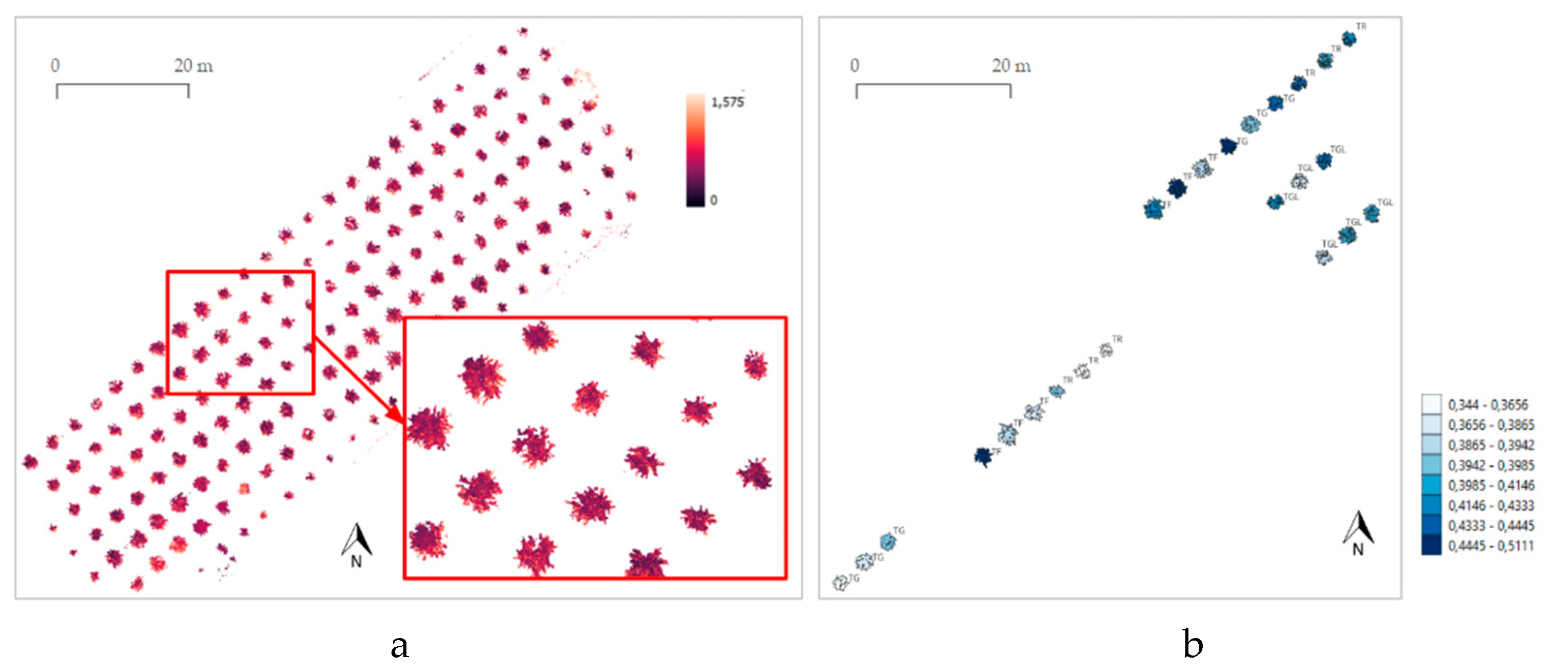
Figure 14.
Relationships between NDVI from P4M and CWSI per each cultivar.

Figure 15.
Visual comparison between the NDVI index and the CWSI index, where the first and the third of each row images represent the NDVI index, and the other images represent the CWSI index. For example, two plants for cultivar are represented in the figure.
Figure 15.
Visual comparison between the NDVI index and the CWSI index, where the first and the third of each row images represent the NDVI index, and the other images represent the CWSI index. For example, two plants for cultivar are represented in the figure.
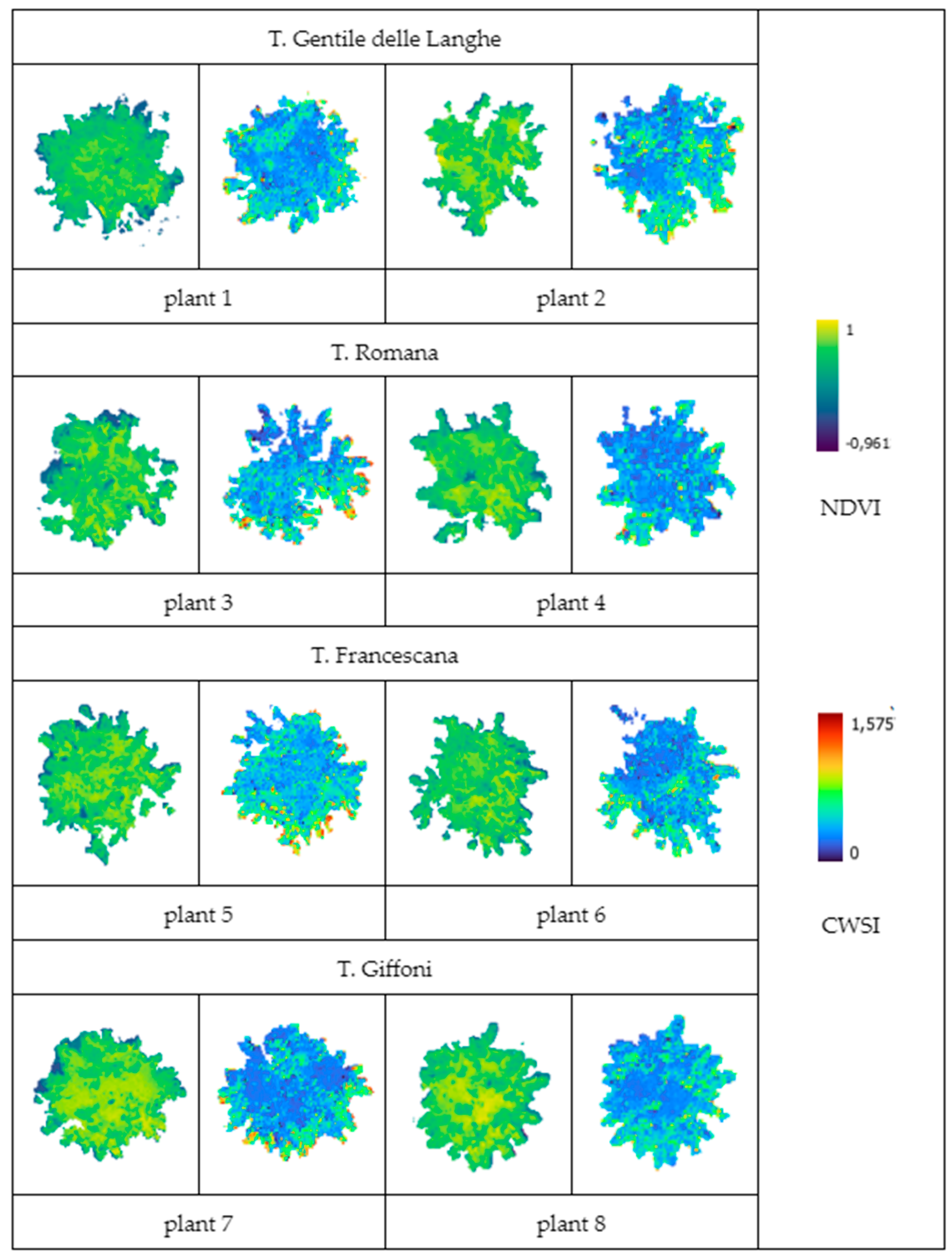

Table 1.
Size traits of tree for each cultivar and average (mean and standard deviation): canopy area, tree height, canopy height and canopy volume obtained from multispectral UAV (P4M) and thermal UAV (M3T) surveys.
Table 1.
Size traits of tree for each cultivar and average (mean and standard deviation): canopy area, tree height, canopy height and canopy volume obtained from multispectral UAV (P4M) and thermal UAV (M3T) surveys.
| Canopy area (m2) | Tree height (m) | Canopy height (m) | Canopy volume (m3) | |||||||||||||
| P4M | M3T | P4M | M3T | P4M | M3T | P4M | M3T | |||||||||
| Cv | Mean | Dev.st. | Mean | Dev.st. | Mean | Dev.st. | Mean | Dev.st. | Mean | Dev.st. | Mean | Dev.st. | Mean | Dev.st | Mean | Dev.st |
| TGL | 1.729 | 0.407 | 1.961 | 0.303 | 2.019 | 0.281 | 2.673 | 0.309 | 1.352 | 0.185 | 1.975 | 0.124 | 2.272 | 0.329 | 3.604 | 0.341 |
| TG | 2.179 | 0.380 | 2.137 | 0.333 | 1.831 | 0.102 | 2.443 | 0.173 | 1.260 | 0.081 | 1.909 | 0.150 | 2.824 | 0.335 | 3.923 | 0.282 |
| TF | 2.557 | 0.432 | 2.606 | 0.359 | 2.078 | 0.043 | 2.814 | 0.049 | 1.520 | 0.096 | 2.296 | 0.164 | 3.593 | 0.473 | 5.231 | 0.303 |
| TR | 1.611 | 0.357 | 1.531 | 0.246 | 1.762 | 0.184 | 2.440 | 0.277 | 1.229 | 0.239 | 1.840 | 0.301 | 1.477 | 0.341 | 2.566 | 0.312 |
| mean | 2.019 | 2.059 | 1.922 | 2.592 | 1.340 | 2.005 | 1.347 | 1.330 | ||||||||
Table 2.
Mean and standard deviation of NDVI for cultivar obtained by P4M survey; Mean and standard deviation of LAI for cultivar obtained by manual measurements.
Table 2.
Mean and standard deviation of NDVI for cultivar obtained by P4M survey; Mean and standard deviation of LAI for cultivar obtained by manual measurements.
| Cultivar | NDVI | LAIm | ||
|---|---|---|---|---|
| Mean | Dev.st. | Mean | Dev.st. | |
| TGL | 0.490 | 0.17 | 2.770 | 0.34 |
| TG | 0.528 | 0.19 | 2.211 | 0.38 |
| TF | 0.477 | 0.18 | 2.083 | 0.43 |
| TR | 0.453 | 0.18 | 2.121 | 0.34 |
Table 3.
△T between canopy temperature, measured by UAV and FLIR thermal camera and air temperature. Different uppercase letters indicate significant (Probability<0.05) differences between the average values of the two survey’s methods. Different lowercase letters indicate significant (Probability<0.05) differences between the average values of the two survey’s methods per each cultivar.
| Cultivar | △T Thermal UAV (°C) | △T Manual (°C) | ||
|---|---|---|---|---|
| Mean | Dev.st. | Mean | Dev.st. | |
| TGL | 3.064 a | 0.862 | 3.633 a | 0.153 |
| TG | 2.183 b | 0.640 | 3.600 a | 0.400 |
| TF | 2.146 a | 1.009 | 2.067 a | 1.929 |
| TR | 1.911 a | 0.992 | 3.400 a | 1.044 |
| Mean | 2.326 B | 3.175 A | ||
Table 4.
Mean and standard deviation of CWSI calculated for each cultivar.
| Cultivar | CWSI | |
|---|---|---|
| Mean | Dev.St. | |
| TGL | 0.406 | 0.024 |
| TG | 0.412 | 0.057 |
| TF | 0.418 | 0.040 |
| TR | 0.395 | 0.038 |
Disclaimer/Publisher’s Note: The statements, opinions and data contained in all publications are solely those of the individual author(s) and contributor(s) and not of MDPI and/or the editor(s). MDPI and/or the editor(s) disclaim responsibility for any injury to people or property resulting from any ideas, methods, instructions or products referred to in the content. |
© 2024 by the authors. Licensee MDPI, Basel, Switzerland. This article is an open access article distributed under the terms and conditions of the Creative Commons Attribution (CC BY) license (http://creativecommons.org/licenses/by/4.0/).
Copyright: This open access article is published under a Creative Commons CC BY 4.0 license, which permit the free download, distribution, and reuse, provided that the author and preprint are cited in any reuse.


