Submitted:
17 February 2024
Posted:
20 February 2024
You are already at the latest version
Abstract
Keywords:
1. Introduction
2. Integration of Renewable Energy Sources to Smart Grids
- Power quality: When RESs are integrated into the grid system, there are various deviations in the rated voltage and frequency, since energy production from RESs also entails intervals of reduced production, because it is based on natural phenomena.
- Power availability: One of the main challenges as well as one of the most important disadvantages of RES is to address the instability of electricity production. Therefore, the possibility of occurrence of detrimental breakdowns during the operation of the system lies.
- Variation in energy production and its speed: As mentioned above, renewable energy technologies do not guarantee stable energy production for the grid, so appropriate measures should be taken in order to avoid major disruptions to the grid. Also, the speed of fluctuation of energy production presents difficulty for this integration.
- Forecast: It is related to electricity production, which is not stable in case of integration of RESs into the grid system.
- Location of renewable energy sources: RES plants depend on climatic conditions, the geographical location of the area and their distance from the grid in terms of cost and performance. Therefore, these settings pose a contest if they are combined into the network system.
- Cost issue: This issue is related to the position of RES stations in the grid system. In fact, most RES plants are located away from the grid system and require energy transmission and consequently transmission lines that depend on the voltage level. Thus, it is very costly to produce electricity through the integration of the RES grid.
3. Intelligent Energy Electricity Systems
3.1. The Traditional Electricity System
3.2. The Future Electricity System
3.3. Infrastructure
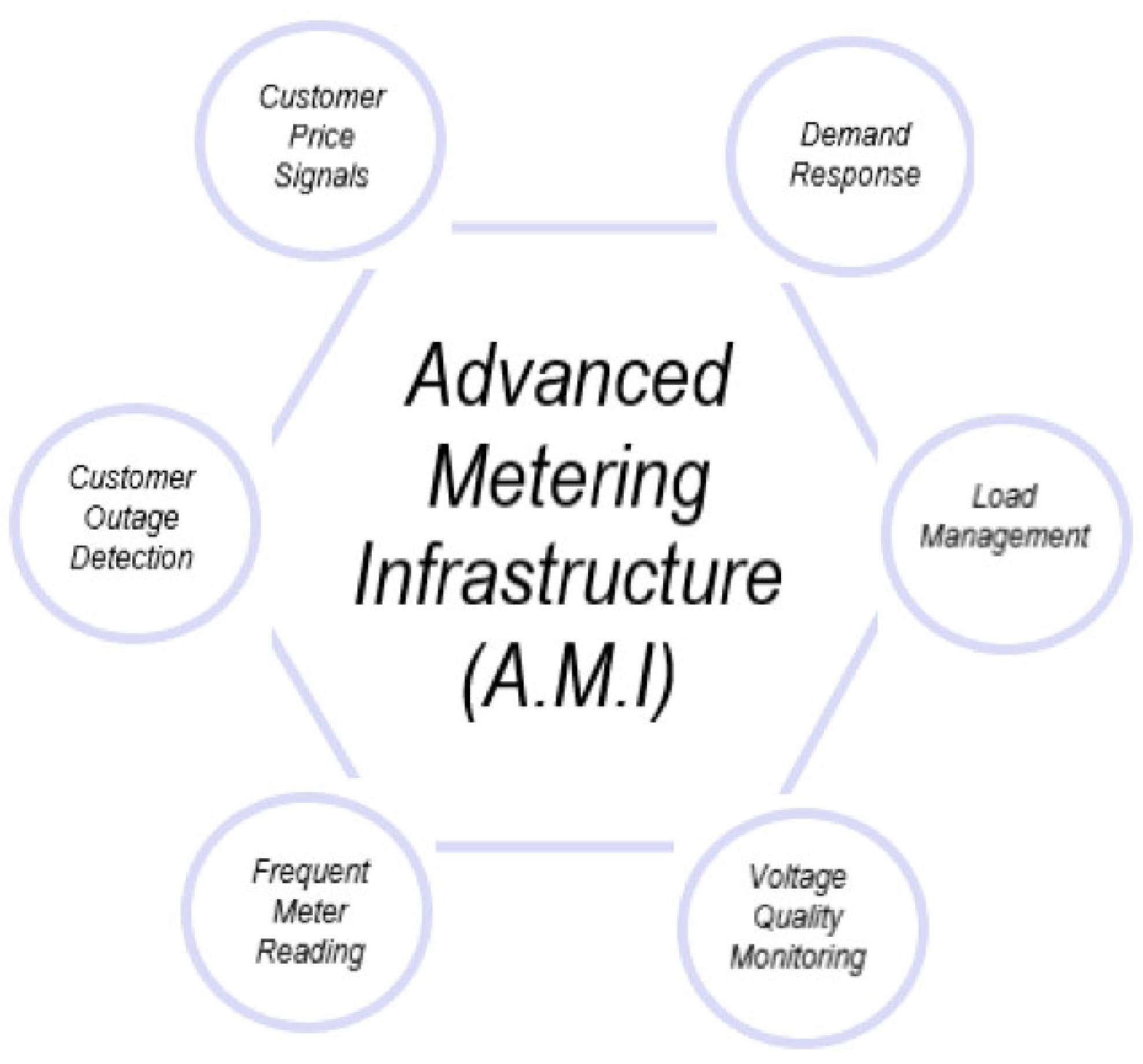
3.3.1. Introduction to Advanced Measurement Infrastructure (AMI)
3.3.2. AMI Security Challenges
- End-user privacy: The routine of patrons can be unprotected by material found from shoppers' electricity ingesting, subsequent in a critical location. Cases of serious info seepage can be in the form of terror and safety schemes used, quantity of people existing in a house, tenure time, kinds of devices, sanctuary, and medical crises.
- System resilience against cyber-attacks: Cybersecurity is acquisition status in SGs due to the snowballing likelihood of cyber-attacks and occurrences. Since the idea of opinion of vulnerability, the aggressor could arrive a smart network and invent mechanisms to subvert the network in several ways that are extremely impulsive. The cybersecurity threats that exist for the security of AMI are as follows:
- Confidentiality: Privacy is unspoken to guard the discretion of shopper data and the way in which it is expended [22]. So, the organization must stipulate for the discretion of ingesting data to be upheld.
- Responsibility: It mentions to the detail that information receivers will not waste to obtain information and vice versa. Time harmonization and precise timestamping of data are vital in the AMI net to safeguard answerability.
- Power theft prevention: The incidence of electrical losses can occur at any of the phases of production, transportation, distribution, and use. Losses happening throughout production are technically more effortlessly defensible than those that happen throughout transportation and distribution. Losses can also be classified as technical and non-technical losses. The usage of SMs in mixture by the AΜΙ in SGs has caused the removal or discount of these issues [23,24].
3.3.3. Smart Meter Features
3.3.4. Phase Measurement Unit (PMU)
3.4. Blockchain Technology Infrastructure
3.4.1. Introduction to Blockchain Technology
- Energy production–In this case blockchain technology provides dispatching organizations with full awareness about the total operating status of an electricity grid in real time. This allows them to growth mission projects that would maximize profits.
- Transmission and distribution of electricity - Blockchain systems allow automation and control centers to have decentralized systems that go beyond the primary challenges noticed in traditional central systems.
- Energy Consumers - Like the production and transmission side, the blockchain could be advantageous on this side under supervision the energy trade between prosumers and various energy storage systems, as well as electric vehicles. Deregulation of the electricity grid has directed to the decentralization of electricity markets around the world. Therefore, a blockchain-based energy trading system is wished-for, which will be secure and reliable to encourage long-term investment [31].
3.5. Telecommunication Interface
3.5.1. Wired Line Communication Technologies
- Power Line Communication (PLC): PLC communication is mainly used for metering applications in internal HANs networks [17]. PLC communication operates in frequency bands from 0.3kHz to 3kHz for ultra-narrow band. However, there are two major PLC communication technologies that operate at different bandwidths, such as Narrowband communication (NB-PLC) and Broadband communication (BB-PLC). Communication (NB-PLC) can be used on both low and high voltage lines with bandwidths ranging from 10kbps to 500kbps and frequency bands from 3kHz to 500kHz. While communication (BB-PLC), operates at significantly higher bandwidths of up to 200Mbps and higher frequency bands from 2MHz to 30MHz [4]. The most important advantage of PLC communication is reliability and sensitivity to interference, while the main problems encountered with PLC communication include interference, noise issues, attenuation and signal distortion caused by distribution transformers, limiting the suitability and widespread use of PLC communication in NANs networks. To overcome this, hybrid grid solutions are proposed where SMs are connected to a data concentrator via power lines and then, in a second stage, wireless technology, e.g. mobile telephony, is used to transfer the aggregated data to the utility data center [17].
- Communication via Fiber Optics (FO): Fiber optic cables offer the potential for relatively long-distance communication without the need for intermediate relays or amplification and are inherently immune to electromagnetic interference. Fiber optics provide data rates (155Mbps - 50Gbps) and a coverage range of 100km. They are advantageous due to their high capacity and reliability, while on the contrary they are disadvantaged in terms of cost and regular maintenance.
3.5.2. Wireless Communication Technologies
- Wireless Local Area Network (WLAN) and Wi-Fi: Wireless Local Area Network (WLAN), which is based on IEEE 802.11, uses spread spectrum technology so that users can occupy the same frequency bands causing minimal interference between them. WLAN is suitable for applications with relatively lower data rate requirements and low interference environments. 802.11-based networks are the most popular for use on a LAN with maximum data rates of 150Mbps and a maximum transmission range of 70m indoors and 250m outdoors. WLAN based on IEC 61850 can enhance the protection of distribution substations through intelligent monitoring and control using sensors and smart controllers with wireless interfaces. Communications for monitoring and control at substations can be made more reliable using wireless connections alongside fiber optics. Wi-Fi is one of the most important technologies based on IEEE 802.11 and used in HAN networks, mobile phones, computers, and many other electronic devices. Wi-Fi technologies operate at 2.4GHz providing maximum data rates of 11Mbps with latency of 3.2-17ms. Data rates up to 600Mbps can be obtained via 802.11n using the multi-input-multi-output (MIMO) scheme [38].
- WiMAX: WiMAX is one of the IEEE 802.16 series standards designed for Metropolitan Area Wireless Network (WMAN) and aims to achieve global interoperability in bandwidth (2-66GHz). WiMAX is characterized by low latency (< 100ms), high data rates, coverage range of tens of kilometers, low development costs, and the ability to cope with normal and extraordinary conditions [38].
- ZigBee: ZigBee is a wireless network based on the IEEE 802.15.4 standard and is an efficient and cost-effective solution. However, it offers a low data rate for Personal Area Networks (PANs). This technology can be widely used in device control, building automation, remote monitoring, healthcare, etc. Estimated data rates are 250kbps per channel on the 2.4GHz unlicensed band, 40kbps per channel on the 915MHz band, and 20kbps per channel on the 868MHz band. ZigBee supports 10-75 m point-to-point and usually 30 m internal and unlimited distance in bronchoid network. Bronchial networks are decentralized, and each node is able to dynamically self-route and connect to new nodes. The features along with low power consumption and low development costs make ZigBee very attractive for home area smart grid (HAN) applications [38].
- 6LoWPAN: 6LoWPAN allows IEEE 802.15.4 (WPAN) and IPv6 to work together to achieve low-power Internet Protocol (IP) networks including sensors, controllers, etc. 6LoWPAN uses loop topology to support high scalability. For example, hierarchical routing is one of the routing protocols used in 6LoWPAN to increase network scalability.
3.5.3. Smart Grid Communication Architecture (WAN, NAN, HAN)
4. 5G Network
4.1. Network Evolution 1G − 5G
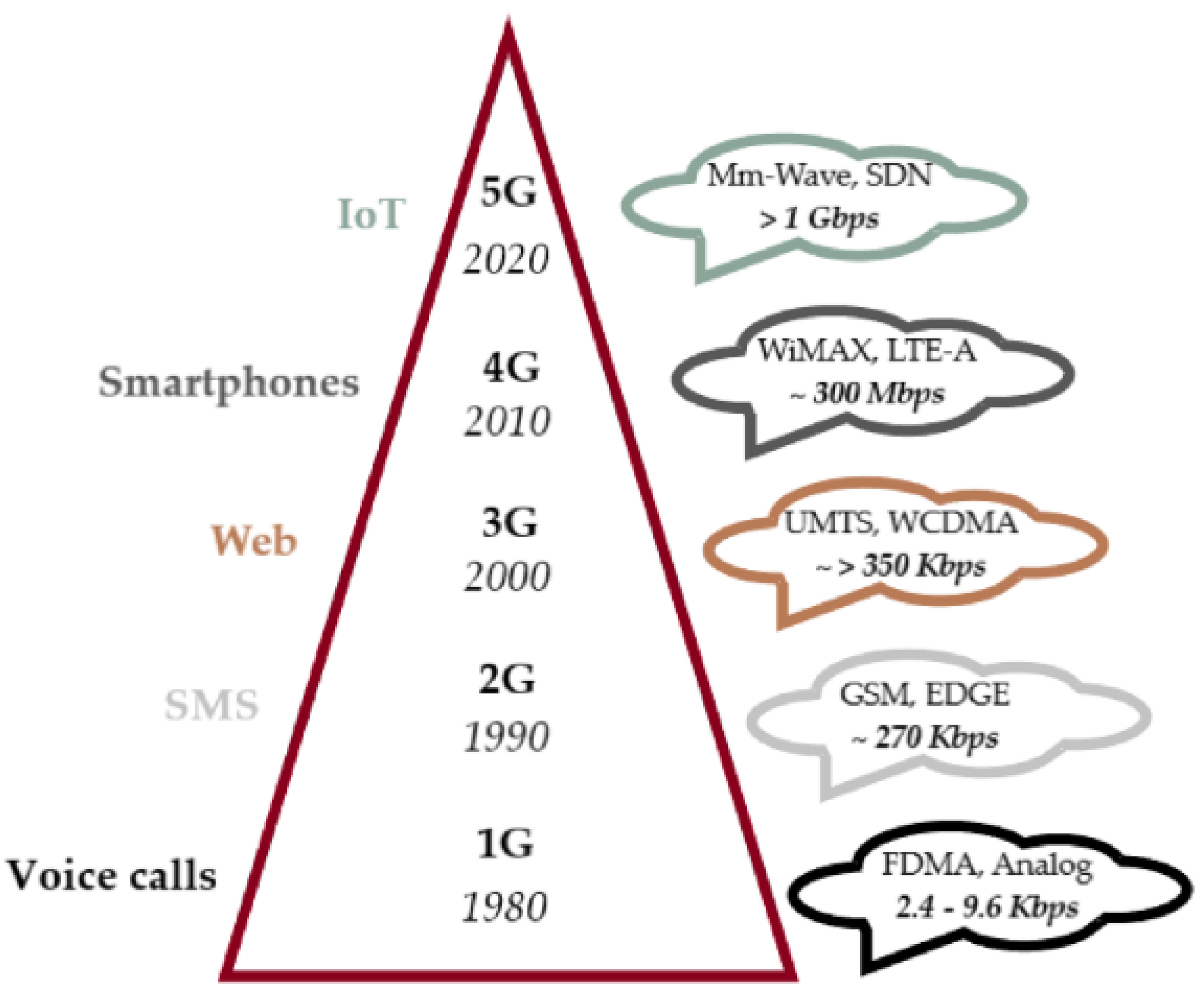
4.2. Main 5G Network Implementation Scenarios
5. Studying and Forecasting of Electrical Loads
5.1. Introduction to Study and Prediction
5.2. Load Curve
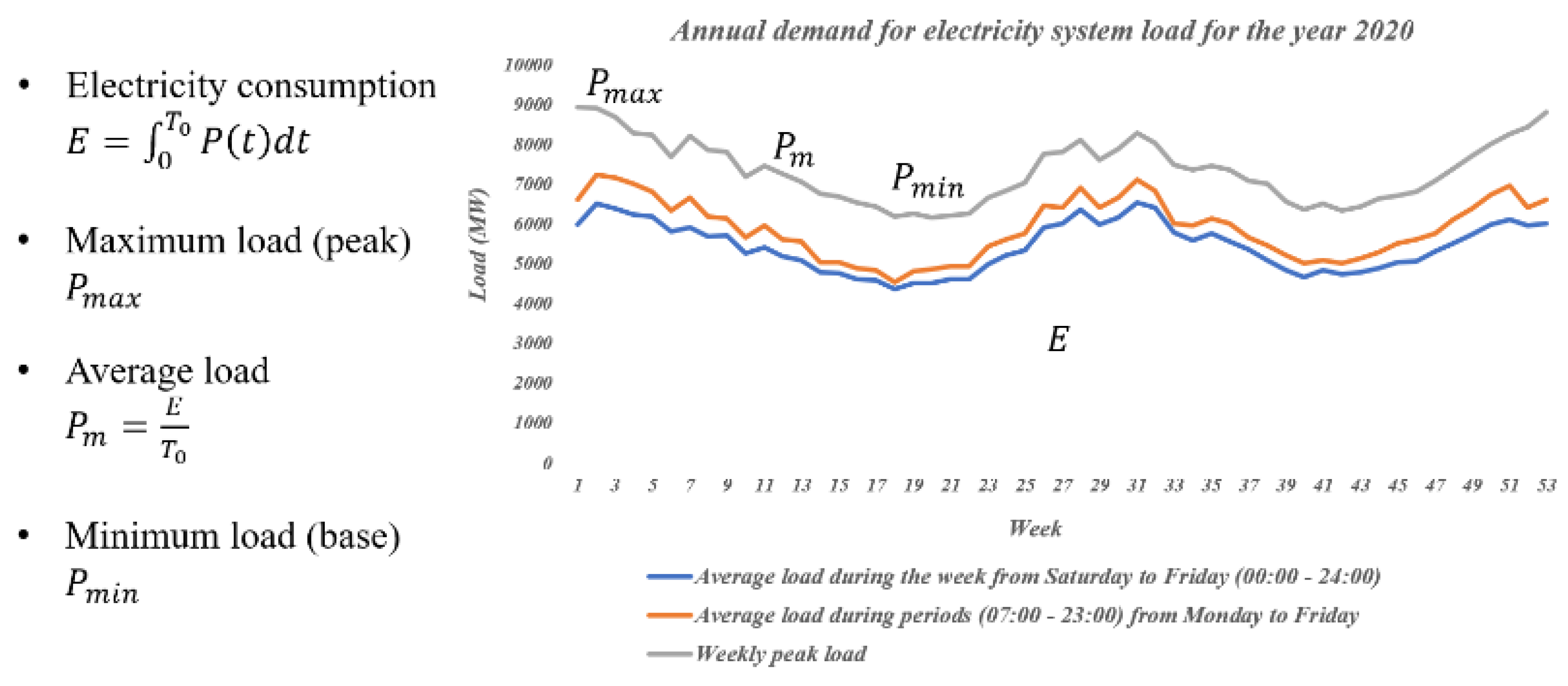
5.3. Load Forecast
5.4. Blockchain Applications in Load Forecast
5.5. Methods and Models for Electrical Load Forecasting
- Autoregressive (AR): The sequences of an auto regurgitated model signifies the aggregate of information essential to predict a predictable signal that can be represented by AR constants. Short-duration acceleration data can certainly be a type of permanent accidental indicator. Consequently, it makes a lot of reason to use the AR model to explain increase of velocity signals. We can then use the AR model measurements as assigns to implement endeavor recognition. The assortment of the model order in AR model is a detailed problem, too low an instruction is a levelled assessment, while too enormous an order affects illegitimate mountains and widespread statistic variability. An AR model is based on special features to recognize activity from triaxial acceleration signals. AR coefficients corresponding to different activity patterns are discriminatory. Also, AR factors can provide sufficient distinction between different types of human activity and provide new feature options for activity recognition [49].
- The MA model is a linear regression model that expresses the declination, of the process as a finite, weighted sum of white noise terms. The unkind model accepts that the top predictor of what will transpire tomorrow is the average of the whole thing that has occurred up until now. The random walk model undertakes that the unsuitable predictor of what will happen tomorrow is what transpired today, and all previous antiquity can be overlooked. Spontaneously there is a range of prospects in involving these two limits. Why not take an average of what has occurred in some window of the latest prior? That’s the concept of a “moving” average [50].
- The Kalman filter (KF) is established as an ideal repair estimator for a linear system. Founded on nonflavored transformation (UT), the UKF algorithm is advanced for nonlinear systems as a recursive state estimator. The unscented transform (UT) is a deterministic sampling technique, which utilizes a set of 2n+1 sample points (called “sigma points”) for the approximation of statistic characteristics of the changed variable. Forecasts, especially long-term ones, are marked by a high layer of uncertainty due to their high reliance on socio-economic agents, so a level of error of up to 10% is permissible. Applying a Kalman algorithm can significantly minimize the average model error. The KF is a set of mathematical equations in the state space that can provide efficient, computational means for estimating the state of an observed process. In addition, this filter is very powerful in various other aspects such as: support for assessing past, present and future situations, but also for controlling noisy systems [47,48].
- A system is called a white system if all the evidence linked with that system is known, and conversely, it is called a black system if all the information is undetermined. Hence, the grey system is a system with partially known and partly unknown information. There are several systems in this world in which social information is either incomplete or challenging to gather. The simplest form of the grey sculpting approach is the Grey Model (GM) (1, 1). The first ‘1’ signifies the order of the differential equation, and the second ‘1’ suggests the number of variable stars. This theory can trade with noticed systems that have semi unknown parameters, as grey models need only a partial amount of data to assess the conduct of the unknown system. GM’s are suitable for all four types of load forecast [54].
- The exponential smoothing (ES) method describes a class of forecasting methods. Each has the property that forecasts are weighted combinations of past observations, where recent observations are given relatively more weight than older ones. The double exponential smoothing (DES) is an extension of ES designed for trend time series. Exponential Smoothing (ES) is a realistic approach to prediction, according to which the forecast can be made from the exponentially weighted average of previous comments. ES models are between the most public and widespread methods of statistical forecast due to their precision, austerity, and petite cost [55].
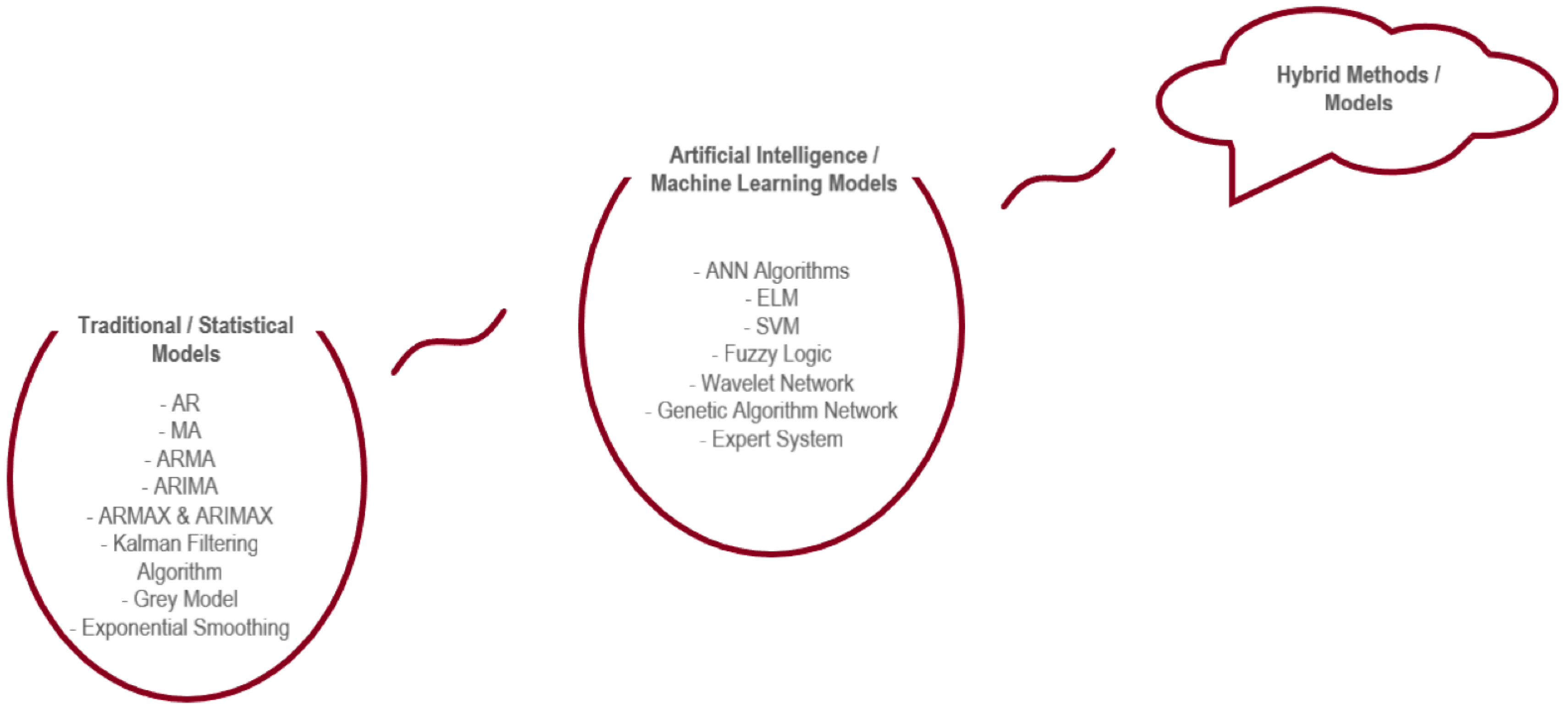
5.6. Contributions of Methods and Models for Electrical Load Forecasting
- High computational complexity: SVM has sharp computational complication and uncertain in processing the indeterminate data [60]. In electricity load forecasting, surplus aspects in data improve the computational difficulty of SVM in its guiding means and lowers the forecast truth.
- Hard to tune parameters: Tremendous parameters of SVM influences the concert of SVM in forecasting. Those parameters are Cost penalty, kernel parameter and reason loss meaning. It is challenging to locate the precise quantities of these parameters for higher precision.
6. Conclusions
7. Proposals for Future Research
7.1. Smooth Transition to the Future Smart Grid (SG)
7.2. Future Research
Abbreviations
| AMI | Advanced Metering Infrastructure |
| AWNNs | Advanced Wavelet Neural Networks |
| AI | Artificial Intelligence |
| ANN | Artificial Neural Network |
| AMR | Automated Meter Reading |
| ARFIMA | Automatic Fractionally Integrated Moving Average |
| AMM | Automatic Meter Management |
| AR | Autoregressive |
| ARIMA | Autoregressive Moving Average |
| ARMA | Autoregressive Moving Average |
| CIS | Consumer Information System |
| DR | Demand Response |
| DERs | Distributed Energy Resources |
| DMS | Distribution Management System |
| DES DTC |
Double Exponential Smoothing Decision Tree Classifier |
| ES | Exponential Smoothing |
| ELF ELM FDI |
Electric Load Forecast Extreme Learning Machine False Data Injection |
| GA | Genetic Algorithm |
| GIS GM |
Geographical Information System Grey Model |
| HAN | Home Area Network |
| HEMS HFSEC HFS |
Home Energy Management System Hybrid Feature Selection, Extraction and Classification Hybrid Feature Selection |
| ICTs | Information and Communication Technologies |
| IENs | Intelligent Electrical Networks |
| IEDs | Intelligent Electronic Devices |
| IRENA | International Renewable Energy Agency |
| IETF | Internet Engineering Task Force |
| IoT | Internet of Things |
| KF | Kalman Filter |
| LAN | Local Area Network |
| mMTC | Mass Machine-Type Communication |
| MIMO | Massive Multiple-Input Multiple-Output |
| MAPE | Mean Average Percentage Error |
| MDMS | Measurement Data Management System |
| mmWAVE | Millimeter-Wave |
| MA | Moving Average |
| NAN | Neighborhood Area Network |
| OMS | Operational Interruption Management System |
| PMU | Phase Measurement Unit |
| QWs | Quantum Cables |
| RESs RFE |
Renewable Energy Sources Recursive Feature Elimination |
| uRLLC | Reliable and Low Latency Communications |
| SLFN | Single Hidden Layer Feedforward Neural Network |
| SG | Smart Grid |
| SM | Smart Meter |
| SVM | Support Vector Machine |
| UT | Unscented Transform |
| VPPs WNN XGBOOST |
Virtual Power Plants Wavelet Neural Network Extreme Gradient Boosting |
References
- Mohussel, R. – R.; Fung, A.; Mohummadi, F.; Raahemifar, K. A survey on advanced metering infrastructure. Electrical and Power Energy System 2014, 63, 473 – 484. [CrossRef]
- Goudarzi, A.; Ghayoor, F.; Waseem, M.; Fahad, S.; Traore, I. A survey on IoT-enabled smart grids: Emerging, applications, challenges, and outlook. Energies 2022, 15, 6984. [CrossRef]
- Moreno Escobar, J.J.; Morales Matamoros, O.; Tejeida Padilla, R.; Lina Reyes, I.; Quintana Espinosa, H. A comprehensive review on smart grids: Challenges and opportunities. Sensors 2021, 21, 6978. [CrossRef]
- Jiang, X.; Wu, L. Residential power scheduling based on cost efficiency for demand response in smart grid. IEEE Access 2020, 8, 197324-197336. [CrossRef]
- Olivares, D.E. et al. Trends in microgrid control. IEEE Trans. Smart Grid 2014, 5, 1905-1919. [CrossRef]
- Kabalci, Y. A survey on smart metering and smart grid communication. Renewable and Sustainable Energy Reviews 2016, 57, 302 – 318. [CrossRef]
- Colak, I.; Sagirogla, S.; Fulli, G.; Yesilbudak, M.; Covrig C. – F. A survey on the critical issues in smart grid technologies. Renewable and Sustainable Energy Reviews 2016, 54, 396 – 405. [CrossRef]
- Chen, Y.; Bhutta, M.S.; Abubakar, M.; Xiao, D.; Almasoudi, F.M.; Naeem, H.; Faheem, M. Evaluation of machine learning models for smart grid parameters: Performance analysis of ARIMA and Bi-LSTM. Sustainability 2023, 15, 8555. [CrossRef]
- Kuppusamy, R.; Nikolovski, S.; Teekaraman, Y. Review of machine learning techniques for power quality performance evaluation in grid-connected systems. Sustainability 2023, 15, 15055. [CrossRef]
- Priyanka, E.B.; Thangavel, S.; Gao, X. Z. Review analysis on cloud computing based smart grid technology in the oil pipeline sensor network system. Petroleum Research (Elsevier) 2021, 6, 77 – 90. [CrossRef]
- Hassan, A.; Afrouzi, H. N.; Siang, C. H.; Ahmed, J.; Mehranzamir, K.; Wooi, C. – L. A survey and bibliometric analysis of different communication technologies available for smart meters. Cleaner Engineering and Technology (Elsevier) 2022, 7, 100-424. [CrossRef]
- Gkonis, P.; Giannopoulos, A.; Trakadas, P.; Masip-Bruin, X.; D’Andria, F. A survey on IoT-edge-cloud continuum systems: Status, challenges, use cases, and open issues. Future Internet 2023, 15, 383. [CrossRef]
- Chen C.; Wang J.; Qiu, F.; Zhao, D. Resilient distribution system by microgrids formation after natural disasters. IEEE Trans. Smart Grid, 2015, 7(2), 958-66. [CrossRef]
- Yuan, W.; Wang, J.; Qiu, F.; Chen, C.; Kang, C.; Zeng, B. Robust optimization-based resilient distribution network planning against natural disasters. IEEE Trans. Smart Grid, 2016, 7(6), 2817-26. [CrossRef]
- Chen J, Zhu Q. A game-theoretic framework for resilient and distributed generation control of renewable energies in microgrids. IEEE Trans. Smart Grid, 2016, 8(1), 285-95. [CrossRef]
- Das, L.; Munikoti, S.; Natarajan, B.; Srinivasan, B. Measuring smart grid resilience: Methods, challenges and opportunities. Renewable and Sustainable Energy Reviews 2020, 130, 109-918. [CrossRef]
- Kalalas, C.; Linus, T.; Zarate, J. A. Cellular communications for smart grid neighborhood area networks: A survey. IEEE Access 2016, 4, 1469-1493. [CrossRef]
- Dorji, S.; Stonier, A.A.; Peter, G.; Kuppusamy, R.; Teekaraman, Y. An extensive critique on smart grid technologies: Recent advancements, key challenges, and future directions. Technologies 2023, 11, 81. [CrossRef]
- Alsuwian, T.; Shahid Butt, A.; Amin, A.A. Smart grid cyber security enhancement: Challenges and solutions—A Review. Sustainability 2022, 14, 14226. [CrossRef]
- Abdul Baseer, M.; Alsaduni, I. A novel renewable smart grid model to sustain solar power generation. Energies 2023, 16, 4784. [CrossRef]
- Naamane, A.; Msirdi, N.K. Towards a smart grid communication. Energy Procedia 2015, 83, 428 – 433. [CrossRef]
- Kua, J.; Hossain, M.B.; Natgunanathan, I.; Xiang, Y. Privacy preservation in smart meters: Current status, challenges and future directions. Sensors 2023, 23, 3697. [CrossRef]
- Ghosal, A.; Conti, M.; Key management systems for smart grid advanced metering infrastructure: A Survey. IEEE Commun. Surv. Tutor. 2019, 21(3), 2831-2848. [CrossRef]
- Leiva, J.; Palacios, A.; Aguado, J. A. Smart metering trends, implications, and necessities: A policy review. Renewable and Sustainable Energy Reviews 2016, 55, 227 – 233. [CrossRef]
- Wang, Y.; Chen, Q.; Hong, T.; Kang, C. Review of smart meter data analytics: Applications, methodologies, and challenges. IEEE Trans. Smart Grid 2019, 10(3), 3125-3148. [CrossRef]
- Asghar, M. R.; Dan, G.; Miorandi, D.; Chlamtac, I. Smart meter data privacy: A Survey. IEEE Commun. Surv. Tutor. 2017, 19(4), 2820-2835. [CrossRef]
- Dileep, G. A survey on smart grid technologies and applications. Renewable Energy 2020, 146, 2589-2625. [CrossRef]
- Hojabri, M.; Dersch, U.; Papaemmanouil, A.; Bosshart, P. A comprehensive survey on phasor measurement unit applications in distribution systems. Energies 2019, 12, 4552. [CrossRef]
- Aderibole, A. et al. Blockchain technology for smart grids: Decentralized NIST conceptual model. IEEE Access 2020, 8, 43177-43190. [CrossRef]
- Alladi, T.; Chamola, V.; Rodrigues, J.J.P.C.; Kozlov, S.A. Blockchain in smart grids: A review on different use cases. Sensors 2019, 19, 4862. [CrossRef]
- Waseem, M.; Adnan Khan, M.; Goudarzi, A.; Fahad, S.; Sajjad, I.A.; Siano, P. Incorporation of blockchain technology for different smart grid applications: Architecture, prospects, and challenges. Energies 2023, 16, 820. [CrossRef]
- Liu, C.; Zhang, X.; Chai, K. – K.; Loo, J.; Chen, Y. A survey on blockchain-enabled smart grids: Advances, applications and challenges. RIET The Institution of Engineering and Technology WILEY, IET Smart Cities 2021, 3, 56 – 78. [CrossRef]
- Chu, T.; An, X.; Zhang, W.; Lu, Y.; Tian, J. Multiple virtual power plants transaction matching strategy based on alliance blockchain. Sustainability 2023. 15, 6939. [CrossRef]
- Xu, G.; Guo, B.; Su, G.; Zheng, X.; Liang, K.; Wong, D. S.; Wang, H. Am I eclipsed? A smart detector of eclipse attacks for Ethereum. Elsevier Computers & Security 2020, 88, 101604. [CrossRef]
- Zhang, Y.; Shi, Q. An intelligente transaction model for energy blockchain based on diversity of subjects. Alex. Eng. J. 2021, 60, 749-756. [CrossRef]
- Gourisetti, S.N.G.; Sebastian-Gardenas, D.J.; Bhattarai, B.; Wang, P.; Widergren, S.; Borkum, M.; Randall, A. Blockchain smart contract reference framework and program logic architecture for transactive energy systems. Appl. Energy 2021, 304, 117860. [CrossRef]
- Zhang, X.; Fan, M. Blockchain-based secure equipment diagnosis mechanism of smart grid. IEEE Access 2018, 6, 66165-66177, . [CrossRef]
- Etimad, F.; Gungor V.C., Nassef Laila, Akkari Nadine, Malik Abbas M.G., Almasri Suleiman Akyildiz Ian F. A survey on wireless sensor networks for smart grid. Computer Communications 2015, 71, 22 – 33. [CrossRef]
- Lee, S.; Azfar Yaqub, M.; Kim, D. Neighbor aware protocols for IoT devices in smart cities—Overview, challenges and solutions. Electronics 2020, 9, 902. [CrossRef]
- Al-Saman, A.; Cheffena, M.; Elijah, O.; Al-Gumaei, Y.A.; Abdul Rahim, S.K.; Al-Hadhrami, T. Survey of millimeter-wave propagation measurements and models in indoor environments. Electronics 2021, 10, 1653. [CrossRef]
- Adoga, H.U.; Pezaros, D.P. Network function virtualization and service function chaining frameworks: A comprehensive review of requirements, objectives, implementations, and open research challenges. Future Internet 2022, 14, 59. [CrossRef]
- Hussain, M.; Shah, N.; Amin, R.; Alshamrani, S.S.; Alotaibi, A.; Raza, S.M. Software-defined networking: Categories, analysis, and future directions. Sensors 2022, 22, 5551. [CrossRef]
- Siddiqi, M.A.; Yu, H.; Joung, J. 5G Ultra-reliable low-latency communication implementation challenges and operational issues with IoT devices. Electronics 2019, 8, 981. [CrossRef]
- Skouras, T.A.; Gkonis, P.K.; Ilias, C.N.; Trakadas, P.T.; Tsampasis, E.G.; Zahariadis, T.V. Electrical vehicles: Current state of the art, future challenges, and perspectives. Clean Technol. 2020, 2, 1-16. [CrossRef]
- Stamatellos, G.; Stamatelos, T. Short-term load forecasting of the greek electricity system. Appl. Sci. 2023, 13, 2719. [CrossRef]
- Independent Power Transmission Operator (IPTO) in the Greek System, https://www.admie.gr/en.
- Khan, A. R.; Mahmood, A.; Safdar, A.; Khan, Z. A.; Khan, N. A. Load forecasting, dynamic pricing and DSM in smart grid: A review. Renewable and Sustainable Energy Reviews 2016, 54, 1311-1322. [CrossRef]
- Hammad, M. A.; Jereb, B.; Rosi, B.; Dragan, D. Method and models for electric load forecasting: A comprehensive review. Logistics & Sustainable Transport 2020, 11(1), 51-76. [CrossRef]
- Gao, Y.; Mosalam, K.M.; Chen, Y.; Wang, W.; Chen, Y. Auto-regressive integrated moving-average machine learning for damage identification of steel frames. Appl. Sci. 2021, 11, 6084. [CrossRef]
- Su, Y.; Cui, C.; Qu, H. Self-attentive moving average for time series prediction. Appl. Sci. 2022, 12, 3602. [CrossRef]
- Rojas, I.; Valenzuela, O.; Rojas, F.; Guillen, A.; Herrera, L.J.; Pomares, H.; Marquez, L.; Pasadas, M. Soft-computing techniques and ARMA model for time series prediction. ScienceDirect 2008, 71, 519-537. [CrossRef]
- Haiges, R.; Wang, Y. D.; Ghoshray, A.; Roskilly, A.P. Forecasting electricity generation capacity in Malaysia: An Auto Regressive Integrated Moving Average approach. ELSEVIER ScienceDirect 8th International Conference on Applied Energy, Energy Procedia 2016, 105, 3471-3478.
- Shilpa, G. N.; Sheshadri, G. S. ARIMAX model for short-term electrical load forecasting. International Journal of Recent Technology and Engineering (IJRTE) 2019, 8(4), 2277-3878.
- Faheemullah Shaikh, Qiang Ji, Pervez Hameed Shaikh, Nayyar Hussain Mirjat, Muhammad Aslam Uqaili. Forecasting China’s natural gas demand based on optimized nonlinear grey models. ELSEVIER, Energy 2017, 140, 941-951.
- Lifeng Wu, Sifeng Liu, Yingjie Yang. Grey double exponential smoothing model and its application on pig price forecasting in China. ELSEVIER Applied Soft Computing 2016, 39, 117-123.
- Karimi, F.; Sultana, S.; Babakan, A. S.; Suthaharan, S. An enhanced support vector machine model for urban expansion prediction. Computers, Environment and Urban Systems (Elsevier) 2019, 75, 61-75.
- A. Taifour Ali, Eisa B. M. Tayeb, Zaria M. Shamseldin. Short Term Electrical Load Forecasting Using Fuzzy Logic. International Journal Of Advancement In Engineering Technology, Management and Applied Science (IJAETMAS) November 2016, Volume 03 – Issue 11, 131 – 138.
- Mashud Rana, Irena Koprinska. Forecasting electricity load with advanced wavelet neural networks. ELSEVIER Neurocomputing 2016, 182, 118-132. [CrossRef]
- C. Bharathi, D. Rekha and V. Vijayakumar. Genetic Algorithm Based Demand Side Management for Smart Grid. CrossMark Wireless Pers Commun 2017, 93, 481-502.
- Zhu, Q., Han, Z., Basar, T. A differential game approach to distributed demand side management in smart grid. IEEE International Conference on Communications 2012, pp. 3345-3350.
- Tongyi Huang, Wu Yang, Jun Wu, IEEE Member, Jin Ma, Xiaofei Zhang, And Daoyin Zhang. A Survey on Green 6G Network: Architecture and Technologies: IEEE Access 2019, Volume 7. [CrossRef]


| Work | Publication Year | Key Contributions |
|---|---|---|
| [2] | 2022 | IoT and SGs |
| [6] | 2016 | Smart metering in SGs |
| [9] | 2023 | ML for load forecasting and power quality improvement |
| [11] | 2022 | Research and analysis of modern communication technologies available for SMs. |
| [18] | 2023 | SG technologies, recent developments, key challenges. |
| [19] | 2022 | Challenges and solutions to improve SG cybersecurity. |
| Our work | - | Communication technolgoies and electric load forecasting for SGs |
| Traditional Grid | Smart Grid |
|---|---|
| One-way Communication | Real-time two-way communication |
| Central Electricity Production Slow Response to Emergency Situations (Manual Control) Limited Control Radial Network Human Intervention in System Disorders Less Data |
Distributed Electricity Production Quick Response to Emergency Situations (Automatic Control) Extensive Control System Dispersed Network Adaptive Protection Large Amount of Data |
| Technology | Achievable Data Rate | Coverage Range | Advantages | Disadvantages |
|---|---|---|---|---|
| Wired Technologies | ||||
| PLC | NB-PLC: 1-10kbps for low data percentage PHYs BB-PLC: 1-10Mbps (up to 200Mbps at a very short distance) |
NB-PLC: 150km or more BB-PLC: ~1,5km | 1. Existing Infrastructure 2. Economics 3. Wide Availability |
1. Channel Noise 2. Interference 3. Attenuation |
| Fiber Optics | ||||
| 155Mbps - 50Gbps | 100km | 1. High Capacity 2. High Reliability 3. High Availability 4. Enhanced Security | 1. High Cost 2. Low Extensibility 3. Development Restrictions 4. Regular Maintenance |
|
| Wireless Technologies | ||||
| Wi-Fi | 11Mbps - 300Mbps | 100m for indoor | 1. Low Cost 2. High Data Rate | 1. Small Range 2. Interference 3. Low Security |
| WiMAX |
|
48km | 1. Low Latency Time 2. Scalability 3. High Data Rate |
1. Non-Wide Use 2. Exclusive Infrastructure 3. Limited Access to Approved Spectrum |
| ZigBee | 20 - 250kbps | 10m - 75m | 1. Low Cost 2. Low Energy Consumption 3. MESH connectivity |
1. Low Data Rate 2. Small Range 3. Interference |
| Forecasting Methods & Models | Advantages | Disadvantages |
|---|---|---|
| Statistical Methods | ||
| Uncomplicated and less computationally expensive. Use to determine relationship between predicted power and weather features. |
Less reliability for large and non-linear data in dataset of energy. Difficult to control complex weather conditions. |
|
| Machine Learning | ||
| Simple and can deal with large datasets. | Less reliability for large and heterogeneous data issues, produce point predictions. | |
| Hybrid Methods | ||
| Highly accurate and scalable. Integrate different model’s weight to improve the performance of model by conserving the advantages of approach | Specific uses. Highly computationally expensive. Face issues of stable prediction due to their complex learning structure. May have long duration of training, under fitting problem and low efficiency. | |
| ARIMA | ||
| Usable for non-linear model. Forecast a regression model and develop a fit. |
Data linearization is needed. Suited to stationary data. Need of data preprocessing. Chance of loss of information. Less accurate for time series data. | |
| ANN | No needs of extra expertise for statistical training. Ability to observe the interaction between independent and dependent variables. Ability to detect all relationships among predictor variables. Can control non-linear interaction in load consumption by adjustment of weight in training process. | Black box in nature. Need of large quantity of datasets to train the model and its complexity. Need data pre-processing and neural networks. |
| Time Series Analysis | Have ability to adopt seasonal effects. | Numerical instability. |
| Fuzzy Inference System | Quick and accurate in execution. | Trail and error-based selection of membership function in the formation of rule. |
Disclaimer/Publisher’s Note: The statements, opinions and data contained in all publications are solely those of the individual author(s) and contributor(s) and not of MDPI and/or the editor(s). MDPI and/or the editor(s) disclaim responsibility for any injury to people or property resulting from any ideas, methods, instructions or products referred to in the content. |
© 2024 by the authors. Licensee MDPI, Basel, Switzerland. This article is an open access article distributed under the terms and conditions of the Creative Commons Attribution (CC BY) license (http://creativecommons.org/licenses/by/4.0/).


