On the Trio Unification of Information Geometry, Einsteinian Relativity, and Transient Queues the Parthasarathian Case

Ismail A Mageed

doi:10.20944/preprints202402.0038.v1

Preprint

Article

On the Trio Unification of Information Geometry, Einsteinian Relativity, and Transient Queues the Parthasarathian Case

This version is not peer-reviewed.

Ismail A Mageed^*

This version is not peer-reviewed.

Downloads

Views

Comments

Submitted:

31 January 2024

Posted:

02 February 2024

You are already at the latest version

Abstract

The current study characterizes the transient M/M/1 queue manifold info-geometrically, through devising Fisher Information matrix(FIM) and its inverse(IFIM). Additionally, the impact of stability on the existence of IFIM and explore the geodesic equations of motion has been revealed. More potentially, the paper discusses the relationship between stability and the Gaussian curvature, as well as the connections between queueing theory, information geometry, , Riemannian geometry, and the Theory of Relativity.

Keywords:

Transient M/M/1

;

statistical manifold (SM)

;

Geodesic equations of motion

;

Riemannian metric (RM)

;

Fisher Information matrix (FIM)

;

Inverse Fisher Information matrix (IFIM)

;

threshold theorem

Subject:

Computer Science and Mathematics - Probability and Statistics

1. Introduction

Numerous study areas, including statistical sciences, have extensively used IG [1]. In other words, the goal of IG is to use statistics to apply the methods of differential geometry (DG), which indicates the major goal of IG is to use stochastic processes and probability theoretic in the applications of methodologies of non-Euclidean geometry.

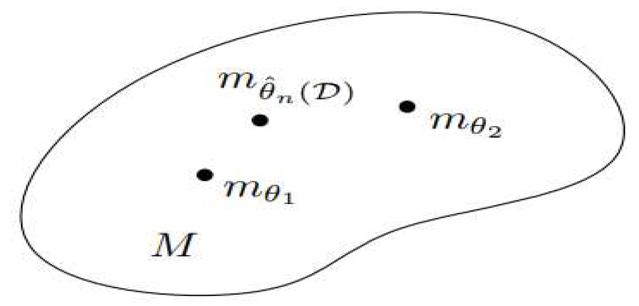
A manifold is a topological finite-dimensional Cartesian space,

R^{n}

, in which an infinite-dimensional manifold exists[2]. Additionally, IG supports SMs’ descriptions that are based on intuitive reasoning. One might have a greater understanding of the crucial significance of IG[3,4]. Parametrization of a Statistical Manifold (SM) is visualized by figure 1[4].

Figure 1. SM’s parametrization(Nielsen 2020).

According to the literature, a paper by[5] examined info-geometrically the stable M/D/1 queue on the basis of queue length routes ‘characteristics, was the real motivator for the current study.

The main deliverables of this paper are described below.

➢: Revealing the new discovery of the geodesic equations of motion of the coordinates of the transient M/M/ $\infty$ .
➢: In the context of the research paper, a novel 𝛼-connection [6] is introduced, which maps each coordinate to a value. The paper also discusses the concept of incompressibility or solenoidality in the transient M/M/1 queue, where closed surfaces have no net flux [7], and includes definitions and physical interpretations of Gaussian and Ricci curvatures.
➢: Revolutionary relativistic and transient queueing theoretic connections are established.

The remainder of the paper is divided into the following sections: Preliminary definitions of Information Geometry (IG) are given in Section 2. The transient M/M/1 QM’s FIM and it IFIM are introduced in Section 3. While Section 5 gives the Information Geometric Equations of Motion (IMEs) for the coordinates of the transient M/M/1 QM, Section 4 addresses the -connection of the queue manifold. The potential function, divergence measurements, stability, and curvature of the M/M/1 QM are all discussed in detail in Sections 6 to 13. Section 14 wraps up the report and provides a plan for further research.

2. Main Definitions

2.1. Main Definition on IG

Definition 1. Statistical Manifold (SM)

M = {p (x, θ) | θ ϵ Θ}

is called an SM[8] if x is a random variable in sample space

X

and

p (x, θ)

is the probability density function, which satisfies certain regular conditions. Here,

θ = (θ_{1}, θ_{2}, . ., θ_{n}) ϵ Θ

is an n-dimensional vector in some open subset

Θ \subset R^{n}

, and

θ

can be viewed as the coordinates on manifold M.

Definition 2. Potential Function

The potential function

Ψ (θ)

(c.f., (2.1)) [8] is the distinguished negative function of the coordinates alone of (

L (x; θ) = l n (p (x; θ))

Definition 3. Fisher’s Information Matrix(FIM)

The FIM (or, Fisher’s metric) [

g_{i j}

][6] is given by the Hessian (the nxn matrix of the partial derivatives of the potential function

Ψ (θ)

with respect to the coordinates) i.e.,

[g_{i j}] = [\frac{\partial^{2}}{\partial θ^{i} \partial θ^{j}} (Ψ (θ))], i, j = 1,2, . ., n

(1)

with respect to natural coordinates.

Definition 4. IFIM

Given the FIM, the inverse matrix of [

g_{i j}

] is defined by[8]

[g^{i j}] = {([g_{i j}]))}^{- 1} = \frac{a d j [g_{i j}]}{∆}

(2)

∆ = \det [g_{i j}]

(3)

Definition 5.

α

-Connection For each

α ϵ R,

the

α

(or

\nabla^{(α)}

)-connection [6] is the torsion-free affine connection with components:

Γ_{i j, k}^{(α)} = (\frac{1 - α}{2}) (\partial_{i} \partial_{j} \partial_{k} (Ψ (θ)))

(4)

where

Ψ (θ)

is the potential function and

\partial_{i}

\frac{\partial}{\partial θ_{i}}

Definition 6.

(1)The geodesic equations of manifold M with coordinate system

θ = (θ_{1}, θ_{2}, . ., θ_{n})

read as [8]

\frac{d^{2} θ^{k}}{d t^{2}} + Γ_{i j}^{k (0)} (\frac{d θ^{i}}{d t}) (\frac{d θ^{j}}{d t}) = 0, i, j = 1,2, \dots, n, Γ_{i j}^{k (α)} = Γ_{i j, s}^{(α)} g^{s k}

(5)

By the above definition, it is clear that the geodesic equations are interpreted physically as the information geometric equations of motion , shortly (IGEMs), or the relativitstic equations of motion (REMs) , or the Riemannian equations of motion.

At this stage, the current study provides a ground- breaking discovery of the IG analysis of transient queueuing systems in comparison to that of non-time dependent queueing systems, namely IG analysis of stable queueues[9,10].

Definition 7.

1. The

α - c u r v a t u r e R i e m a n n i a n

Tensors,

R_{i j k l}^{(α)}

[6] read as:

R_{i j k l}^{(α)} = [(\partial_{j} Γ_{i k}^{s (α)} - \partial_{i} Γ_{j k}^{s (α)}) g_{s l} + (Γ_{j β, l}^{(α)} Γ_{i k}^{β (α)} - Γ_{i β, l}^{(α)} Γ_{j k}^{β (α)})], i, j, k, l, s, β = 1,2, 3, \dots ., n

(6)

Where

Γ_{i j}^{k (α)} = Γ_{i j, s}^{(α)} g^{s k}

(7)

K_{1212}^{(α)}

K^{(α)}

α - G a u s s i a n c u r v a t u r e

and reads as [6]

K^{(α)} = \frac{R_{1212}^{(α)}}{d e t (g_{i j})}

(8)

Definition 8.

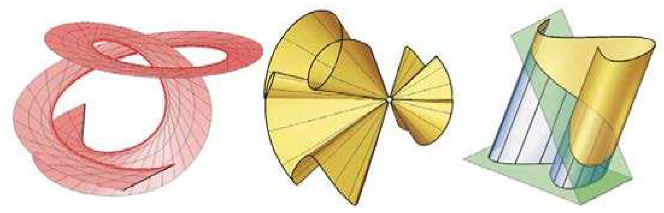
(i) Developable surfaces are a specific class of ruled surfaces that may be mapped onto a flat surface without the curves being altered in any way; each curve is generated from such a surface and keeps its original shape [11].

Figure 2. Three kinds of developable surfaces: Tangential on Figure. 5a (on the left), Conical on Fig. 5b (on the centre) and Figure. 5c (on the right), Cylindrical. Note that curves in bold are directrix or base curves and straight lines in bold are directors or generating lines (curves) [11].

Definition 9.

In mathematics, a function is considered well-defined if it consistently produces the same output regardless of how the input is represented. This means that even if the input is expressed differently, if the value remains the same, the function will yield the same result. This concept ensures the reliability and consistency of mathematical operations and calculations.

Definition 10 [13].

1. function f is said to be one-to-one, or injective, if and only if

f (x) = f (y)

implies

x = y

for all x, y in the domain of

f

. A function is said to be an injection if it is one-to-one. Alternative: A function is one-to-one if and only if

f (x) \neq f (y)

, whenever x ≠ y. This is the contrapositive of the definition.

2.A function f from A to B is called onto, or surjective, if and only if for every

b \in B

there is an element

a \in A

such that

f (a) = b

. Alternative: all co-domain elements are covered.

3. A function f is called a bijection if it is both one-to-one (injection) and onto (surjection).

Theorem 1

[14] Let f be a function that is defined and differentiable on an open interval (c,d).

If f^{'} (x) > 0 (< 0) for all x \in (c, d), then f is increasing (decreasing) on (c, d) .

(9)

Taylor expansions [15]) are widely used to approximate functions by expansions. We have for all

x

around zero,

\ln (1 + x) = \sum_{n = 1}^{\infty} {(- 1)}^{n + 1} \frac{x^{n}}{n}

(10)

\frac{1}{1 + x} = \sum_{n = 0}^{\infty} {(- 1)}^{n} x^{n}

(11)

2.2. Important Inequalities [16]

1. Chebyshev inequality

\frac{x}{1 + x} \leq \ln (1 + x) \leq x f o r x \geq - 1

(12)

(12) can be rewritten as

1 - \frac{1}{x} \leq \ln (x) \leq x - 1 f o r x \geq - 1

(13)

2. Lehmer inequality

\frac{x^{n}}{n!} < \frac{x^{n}}{n!} + 1 \leq e^{x} for all x, n > 0

(14)

3. Fim and Ifim of the Transient M/M/1QM

A single-channel model with exponential inter-arrival times, service times, and FIFO queue discipline is the simplest probabilistic queueing model that can be addressed analytically. In queueing theory, this is referred to as the M/M/1 queue [17].

Based on the introduction of the function, Parthasarathy[18] suggested a straightforward method for the transient solution of the M/M/1 system to read as:

p_{n} (t) = ρ p_{0} (t) e^{- (λ + μ) t} [{\sum_{m = 1}^{n} r_{m} (t) + e}^{(λ + μ) t}], n = 0,1, 2, \dots .

(15)

where

λ

stands for the mean rate per unit time at which arrival instants occur,

μ

is the mean rate of service time,

ρ = \frac{λ (t)}{μ (t)}

defines the traffic intensity or utilisation factor,

r_{n} (t) = μ β_{2}^{n - a_{1}} (1 - δ_{0 a_{1}}) [I_{n - a_{1}} (β_{1} t) - I_{n + a_{1}} (β_{1} t)] + λ β_{2}^{n - 1 - a_{1}} (I_{n + 1 - a_{1}} (β_{1} t) - I_{n - 1 - a_{1}} (β_{1} t))

(16)

w i t h β_{1} = 2 \sqrt{λ μ}, β_{2} = 2 \sqrt{\frac{λ}{μ}}

I_{n} (x)

[19] is the modified Bessel function.

And

p_{0} (t) = \int_{0}^{t} r_{1} e^{- (λ + μ) y} d y + δ_{0 a_{1}}

Theorem 2.

The underlying queue of (15) has:

(i) FIM reads as

[g_{i j}] = [\begin{matrix} a & b & c \\ b & 0 & h \\ c & h & l \end{matrix}]

(17)

where

a = \frac{1}{ρ^{2}} - \frac{1}{{(1 - ρ)}^{2}}

(18)

b = t

(19)

c = \frac{ρ^{.}}{ρ^{2}} + \frac{ρ^{.}}{{(1 - ρ)}^{2}} + t μ^{.} + μ ρ^{.}

(20)

h = (1 + ρ) + t ρ^{.}

(21)

l = \frac{ρ^{. 2} - ρ ρ^{. .}}{ρ^{2}} + \frac{ρ^{. 2} + (1 - ρ) ρ^{. .}}{{(1 - ρ)}^{2}} + ((1 + ρ) t μ^{. .} + μ + {2 ρ}^{.} μ^{.} + 2 μ ρ^{.} + 2 ρ μ^{.} + μ t ρ^{. .}

(22)

Δ = d e t ([g_{i j}])

(23)

= (a (- h^{2}) - b (b l - c h) + c (b h))

(24)

Provided that, . refers to the temporal derivative

\frac{d}{d t}

(iii) [

g^{i j}

] reads as

[g^{i j}] = \frac{a d j [g_{i j}]}{∆} = [\begin{matrix} A & B & L \\ B & E & F \\ L & F & H \end{matrix}]

(25)

where

A = \frac{(- h^{2})}{∆}

(26)

B = \frac{(c h - b l)}{∆}

(27)

L = \frac{(b h)}{∆}

(28)

E = \frac{(a l - c^{2})}{∆}

(29)

F = \frac{(b c - a h)}{∆}

(30)

H = \frac{(- b^{2})}{∆}

(31)

Proof.

(i)Following (15), we have:

L (x; θ) = l n (p_{n} (x; θ)) = l n (ρ p_{0} (t) e^{- (λ + μ) t}) + l n (ρ p_{0} (t) e^{- (λ + μ) t} [{\sum_{m = 1}^{n} r_{m} (t) + e}^{(λ + μ) t}])

(32)

θ = {(θ}_{1}, θ_{2}, θ_{3}) = (ρ, μ, t)

(33)

We have

Ψ (θ) = - l n (ρ) - l n (1 - ρ) + μ (1 + ρ) t, p_{0} (t) = 1 - ρ

(34)

Thus,

\partial_{1} = \frac{\partial Ψ}{\partial ρ} = - \frac{1}{ρ} + \frac{1}{(1 - ρ)} + μ t, \partial_{2} = \frac{\partial Ψ}{\partial μ} = (1 + ρ) t, \partial_{3} = \frac{\partial Ψ}{\partial t} = - \frac{ρ^{.}}{ρ} + \frac{ρ^{.}}{(1 - ρ)} + (1 + ρ) t μ^{.} + μ (1 + ρ) + μ t ρ^{.}

(35)

\partial_{1} \partial_{1} = \frac{1}{ρ^{2}} - \frac{1}{{(1 - ρ)}^{2}} \partial_{1} \partial_{2} = \partial_{2} \partial_{1} = t, \partial_{2} \partial_{2} = 0, \partial_{1} \partial_{3} = \frac{ρ^{.}}{ρ^{2}} + \frac{ρ^{.}}{{(1 - ρ)}^{2}} + t μ^{.} + μ ρ^{.} = \partial_{3} \partial_{1}, \partial_{2} \partial_{3} = (1 + ρ) + t ρ^{.} = \partial_{3} \partial_{2}, \partial_{3} \partial_{3} = \frac{ρ^{. 2} - ρ ρ^{. .}}{ρ^{2}} + \frac{ρ^{. 2} + (1 - ρ) ρ^{. .}}{{(1 - ρ)}^{2}} + (1 + ρ) t μ^{. .} + μ + {2 ρ}^{.} μ^{.} + 2 μ ρ^{.} + 2 ρ μ^{.} + μ t ρ^{. .}

(36)

Therefore, the Fisher Information Matrix, FIM, is obtained (c.f., (17)).

Thus (ii) follows.

[

g^{i j}

] reads as:

[g^{i j}] {= [g_{i j}]}^{- 1} = \frac{a d j [g_{i j}]}{∆} = \frac{T r a n s p o s e (C o v [g_{i j}])}{∆} = \frac{1}{∆} t r a n s p o s e (C o v [\begin{matrix} a & b & c \\ b & 0 & h \\ c & h & l \end{matrix}])

(37)

= [\begin{matrix} (- h^{2}) & (c h - b l) & (b h) \\ (c h - b l) & (a l - c^{2}) & (b c - a h) \\ (b h) & (b c - a h) & (- b^{2}) \end{matrix}]

(38)

Thus,

[g^{i j}] = \frac{1}{∆} t r a n s p o s e (C o v [\begin{matrix} (- h^{2}) & (c h - b l) & (b h) \\ (c h - b l) & (a l - c^{2}) & (b c - a h) \\ (b h) & (b c - a h) & (- b^{2}) \end{matrix}]) = [\begin{matrix} A & B & L \\ B & E & F \\ L & F & H \end{matrix}]

(39)

It is notable that the Fisher Information Matrix, FIM should satisfy the symmetry requirement.

In the following section, the components of

α

(or

\nabla^{(α)}

)- connection are obtained. These calculated expressions are needed to obtain the corresponding Geodesic Equations (GEs) of the parametric coordinates of M/M/1 QM.

4. Connection of the Transient M/M/1 QM

4.1. The Obtained $Γ_{i j, k}^{(α)}$ Expressions (c.f., Equation (4)) of the Transient M/M/1 QM

From (4), the reader can check that:

Γ_{11,1}^{(α)} = - (1 - α) (\frac{1}{{(1 - ρ)}^{3}} + \frac{1}{ρ^{3}})

(40)

0 = Γ_{22,2}^{(α)} = Γ_{12,2}^{(α)} = Γ_{22,1}^{(α)} = Γ_{21,2}^{(α)} = Γ_{11,2}^{(α)} = Γ_{12,1}^{(α)} = Γ_{21,1}^{(α)} = Γ_{22,3}^{(α)} = Γ_{23,2}^{(α)} = Γ_{32,2}^{(α)}

(41)

Γ_{31,1}^{(α)} = (1 - α) ρ^{.} (\frac{1}{{(1 - ρ)}^{3}} - \frac{1}{ρ^{3}})

(42)

Γ_{13,1}^{(α)} = Γ_{11,3}^{(α)} = (1 - α) ρ^{.} (\frac{1}{{(1 - ρ)}^{3}} - \frac{1}{ρ^{3}})

(43)

Γ_{13,2}^{(α)} = Γ_{12,3}^{(α)} = \frac{(1 - α)}{2}

(44)

Γ_{13,3}^{(α)} = \frac{(1 - α)}{2} [\frac{ρ^{. .}}{ρ^{2}} + \frac{ρ^{. .}}{{(1 - ρ)}^{2}} + \frac{{2 ρ}^{. 2}}{{(1 - ρ)}^{3}} + t μ^{. .} + 2 μ^{.}]

(45)

Γ_{23,1}^{(α)} = Γ_{21,3}^{(α)} = \frac{(1 - α) ρ^{.}}{2}

(46)

Γ_{23,3}^{(α)} = \frac{(1 - α) (1 + 2 ρ^{.} + t ρ^{. .})}{2}

(47)

Γ_{31,2}^{(α)} = Γ_{32,1}^{(α)} = \frac{(1 - α)}{2}

(48)

Engaging the same procedure, the remaining components can be determined.

5. THE IMEs OF THE COORDINATES THE TRANSIENT M/M/1 QM

5.1. The $I M E s$ of the $s e r v e r u t i l i z a t i o n$ coordinate, $ρ$ of the transient M/M/1 QM

The IMEs (c.f., Equation (5)) corresponding to the

a r r i v a l r a t e

coordinate,

ρ

of the transient M/M/1 QM are:

\frac{d^{2} θ^{1}}{d t^{2}} + Γ_{i j}^{1 (0)} (\frac{d θ^{i}}{d t}) (\frac{d θ^{j}}{d t}) = 0, i, j = 1,2, 3

(49)

Now, we are in a situation of trying to find the path of motion of family of families of IMEs corresponding to the server utilization coordinate,

ρ .

\begin{matrix} [\frac{d^{2} ρ}{d t^{2}} + [\frac{L}{2} + \frac{L ρ^{.}}{2}] (\frac{d ρ}{d t}) (\frac{d μ}{d t}) + [\frac{1}{2} 2 A ρ^{.} (\frac{1}{{(1 - ρ)}^{3}} - \frac{1}{ρ^{3}}) + B + L [\frac{ρ^{. .}}{ρ^{2}} + \frac{ρ^{. .}}{{(1 - ρ)}^{2}} + \frac{{2 ρ}^{. 2}}{{(1 - ρ)}^{3}} + \\ t μ^{. .} + 2 μ^{.}]) + \frac{1}{2} (2 {A ρ}^{.} (\frac{1}{{(1 - ρ)}^{3}} - \frac{1}{ρ^{3}}) + B + (\frac{ρ ρ^{. .} - {2 ρ}^{. 2}}{ρ^{3}} + \frac{{2 ρ}^{. 2} + (1 - ρ) ρ^{. .}}{{(1 - ρ)}^{3}} + t μ^{. .} + ρ^{.} μ^{.} + \\ μ^{.} + μ ρ^{. .}) L))] (\frac{d ρ}{d t}) (\frac{d t}{d t}) + {[ρ^{.} L (\frac{1}{{(1 - ρ)}^{3}} - \frac{1}{ρ^{3}})] (\frac{d ρ}{d t})}^{2} + [\frac{1}{2} (A ρ^{.} + B (1 + 2 ρ^{.} + t ρ^{. .})) + \\ \frac{1}{2} (A + (ρ^{.} + t ρ^{. .}) L)] (\frac{d μ}{d t}) (\frac{d t}{d t}) + [\frac{1}{2} ((\frac{ρ ρ^{. .} - {2 ρ}^{. 2}}{ρ^{3}} + \frac{{2 ρ}^{. 2} + (1 - ρ) ρ^{. .}}{{(1 - ρ)}^{3}} + t μ^{. .} + ρ^{.} μ^{.} + μ^{.} + \\ μ ρ^{. .}) A + (ρ^{.} + t ρ^{. .}) B + [\frac{{(ρ}^{.} ρ^{. .} - ρ ρ^{\dots}) ρ - 2 ρ^{.} {(ρ}^{. 2} - ρ ρ^{. .})}{ρ^{3}} + \\ \frac{{(ρ}^{.} ρ^{. .} + (1 - ρ) ρ^{\dots}) (1 - ρ) {+ {2 ρ}^{.} (ρ}^{. 2} + (1 - ρ) ρ^{. .})}{{(1 - ρ)}^{3}} + (1 + ρ) t μ^{. . .} + (1 + ρ) μ^{. .} + 3 ρ^{.} μ^{. .} + μ^{.} + {2 ρ}^{. .} μ^{.} + \\ 2 μ ρ^{. .} + 4 μ^{.} ρ^{.} + 2 ρ μ^{. .} + μ t ρ^{. . .} + μ ρ^{. .} + μ^{.} t ρ^{. .}] L)] {(\frac{d t}{d t})}^{2}] = 0 \end{matrix}

(50)

It can be verified that one of the closed form solutions of (5.1) is determined by the paths of motion:

ρ (t) = c o n s t a n t, μ (t) = c o n s t a n t such that ρ \in (0,1), μ > 1

(51)

5.2. The $I M E s$ of the $M e a n s e r v i c e R a t e$ coordinate, $μ$ of the transient M/M/1 QM

The IMEs (c.f., Equation (5)) corresponding to the

m e a n s e r v i c e r a t e

coordinate,

μ

of the transient M/M/1 QM are

\frac{d^{2} θ^{2}}{d t^{2}} + Γ_{i j}^{1 (0)} (\frac{d θ^{i}}{d t}) (\frac{d θ^{j}}{d t}) = 0, i, j = 1,2, 3

Now, we are in a situation of trying to find the path of motion of family of families of IMEs corresponding to the mean service rate,

μ .

[\frac{d^{2} μ}{d t^{2}} + [\frac{F}{2} + \frac{F ρ^{.}}{2}] (\frac{d ρ}{d t}) (\frac{d μ}{d t}) + [\frac{1}{2} (2 B ρ^{.} (\frac{1}{{(1 - ρ)}^{3}} - \frac{1}{ρ^{3}}) + E + F [\frac{ρ^{. .}}{ρ^{2}} + \frac{ρ^{. .}}{{(1 - ρ)}^{2}} + \frac{{2 ρ}^{. 2}}{{(1 - ρ)}^{3}} + t μ^{. .} + 2 μ^{.}]) + \frac{1}{2} (2 {B ρ}^{.} (\frac{1}{{(1 - ρ)}^{3}} - \frac{1}{ρ^{3}}) + E + (\frac{ρ ρ^{. .} - {2 ρ}^{. 2}}{ρ^{3}} + \frac{{2 ρ}^{. 2} + (1 - ρ) ρ^{. .}}{{(1 - ρ)}^{3}} + t μ^{. .} + ρ^{.} μ^{.} + μ^{.} + μ ρ^{. .}) F)] (\frac{d μ}{d t}) (\frac{d t}{d t}) + {[ρ^{.} (\frac{1}{{(1 - ρ)}^{3}} - \frac{1}{ρ^{3}}) F] (\frac{d ρ}{d t})}^{2} + [\frac{1}{2} (B ρ^{.} + E (1 + 2 ρ^{.} + t ρ^{. .})) + \frac{1}{2} (B + (ρ^{.} + t ρ^{. .}) F)] (\frac{d ρ}{d t}) (\frac{d t}{d t}) + [\frac{1}{2} ((\frac{ρ ρ^{. .} - {2 ρ}^{. 2}}{ρ^{3}} + \frac{{2 ρ}^{. 2} + (1 - ρ) ρ^{. .}}{{(1 - ρ)}^{3}} + t μ^{. .} + ρ^{.} μ^{.} + μ^{.} + μ ρ^{. .}) B + (ρ^{.} + t ρ^{. .}) E + [\frac{{(ρ}^{.} ρ^{. .} - ρ ρ^{\dots}) ρ - 2 ρ^{.} {(ρ}^{. 2} - ρ ρ^{. .})}{ρ^{3}} + \frac{{(ρ}^{.} ρ^{. .} + (1 - ρ) ρ^{\dots}) (1 - ρ) {+ {2 ρ}^{.} (ρ}^{. 2} + (1 - ρ) ρ^{. .})}{{(1 - ρ)}^{3}} + (1 + ρ) t μ^{\dots} + (1 + ρ) μ^{. .} + 3 ρ^{.} μ^{. .} + μ^{.} + {2 ρ}^{. .} μ^{.} + 2 μ ρ^{. .} + 4 μ^{.} ρ^{.} + 2 ρ μ^{. .} + μ t ρ^{. . .} + μ ρ^{. .} + μ^{.} t ρ^{. .}] F)] {(\frac{d t}{d t})}^{2}] = 0

(52)

Let

ρ = c o n s t a n t, t h e n (52) r e d u c e s t o

[\frac{d^{2} μ}{d t^{2}} + [\frac{1}{2} (E + F [t μ^{. .} + 2 μ^{.}]) + E + (t μ^{. .} + μ^{.}) F]] (\frac{d μ}{d t}) + [\frac{1}{2} ((t μ^{. .} + μ^{.}) B + [(1 + ρ) t μ^{. . .} + (1 + ρ) μ^{. .} + μ^{.} + 2 ρ μ^{. .}] F)]] = 0

(53)

Δ = d e t ([g_{i j}]) = ((\frac{1}{ρ^{2}} - \frac{1}{{(1 - ρ)}^{2}}) (- {((1 + ρ))}^{2}) - (t^{2} [((1 + ρ) t μ^{. .} + μ + 2 ρ μ^{.}]))

(54)

\begin{matrix} B = \frac{(t μ^{.} (1 - ρ) - t [((1 + ρ) t μ^{. .} + μ])}{∆} \\ = \frac{(t μ^{.} (1 - ρ) - t [((1 + ρ) t μ^{. .} + μ])}{((\frac{1}{ρ^{2}} - \frac{1}{{(1 - ρ)}^{2}}) (- {((1 + ρ))}^{2}) - (t^{2} [((1 + ρ) t μ^{. .} + μ + 2 ρ μ^{.}]))} \end{matrix}

(55)

E = \frac{(a l - c^{2})}{∆} = \frac{((\frac{1}{ρ^{2}} - \frac{1}{{(1 - ρ)}^{2}}) [((1 + ρ) t μ^{. .} + μ + 2 ρ μ^{.}] - {(t μ^{.})}^{2})}{((\frac{1}{ρ^{2}} - \frac{1}{{(1 - ρ)}^{2}}) (- {((1 + ρ))}^{2}) - (t^{2} [((1 + ρ) t μ^{. .} + μ + 2 ρ μ^{.}]))}

(56)

F = \frac{(b c - a h)}{∆} = \frac{(t (t μ^{.}) - (\frac{1}{ρ^{2}} - \frac{1}{{(1 - ρ)}^{2}}) (1 + ρ))}{((\frac{1}{ρ^{2}} - \frac{1}{{(1 - ρ)}^{2}}) (- {((1 + ρ))}^{2}) - (t^{2} [((1 + ρ) t μ^{. .} + μ + 2 ρ μ^{.}]))}

(57)

Following the above done calculations, we have

[\frac{d^{2} μ}{d t^{2}} + [\frac{1}{2} (\frac{((\frac{1}{ρ^{2}} - \frac{1}{{(1 - ρ)}^{2}}) [((1 + ρ) t μ^{. .} + μ + 2 ρ μ^{.}) - {(t μ^{.})}^{2}]}{((\frac{1}{ρ^{2}} - \frac{1}{{(1 - ρ)}^{2}}) (- {((1 + ρ))}^{2}) - (t^{2} [((1 + ρ) t μ^{. .} + μ + 2 ρ μ^{.})))} + \frac{(t (t μ^{.}) - (\frac{1}{ρ^{2}} - \frac{1}{{(1 - ρ)}^{2}}) (1 + ρ))}{((\frac{1}{ρ^{2}} - \frac{1}{{(1 - ρ)}^{2}}) (- {((1 + ρ))}^{2}) - (t^{2} [((1 + ρ) t μ^{. .} + μ + 2 ρ μ^{.}]))} [t μ^{. .} + 2 μ^{.}]) + \frac{(t (t μ^{.}) - (\frac{1}{ρ^{2}} - \frac{1}{{(1 - ρ)}^{2}}) (1 + ρ))}{((\frac{1}{ρ^{2}} - \frac{1}{{(1 - ρ)}^{2}}) (- {((1 + ρ))}^{2}) - (t^{2} [((1 + ρ) t μ^{. .} + μ + 2 ρ μ^{.}]))} + (t μ^{. .} + μ^{.}) \frac{(t (t μ^{.}) - (\frac{1}{ρ^{2}} - \frac{1}{{(1 - ρ)}^{2}}) (1 + ρ))}{((\frac{1}{ρ^{2}} - \frac{1}{{(1 - ρ)}^{2}}) (- {((1 + ρ))}^{2}) - (t^{2} [((1 + ρ) t μ^{. .} + μ + 2 ρ μ^{.}]))})] (\frac{d μ}{d t}) + [\frac{1}{2} ((t μ^{. .} + μ^{.}) \frac{(t μ^{.} (1 - ρ) - t [((1 + ρ) t μ^{. .} + μ])}{((\frac{1}{ρ^{2}} - \frac{1}{{(1 - ρ)}^{2}}) (- {((1 + ρ))}^{2}) - (t^{2} [((1 + ρ) t μ^{. .} + μ + 2 ρ μ^{.}]))} + [(1 + ρ) t μ^{\dots} + (1 + ρ) μ^{. .} + μ^{.} + 2 ρ μ^{. .}] \frac{(t (t μ^{.}) - (\frac{1}{ρ^{2}} - \frac{1}{{(1 - ρ)}^{2}}) (1 + ρ))}{((\frac{1}{ρ^{2}} - \frac{1}{{(1 - ρ)}^{2}}) (- {((1 + ρ))}^{2}) - (t^{2} [((1 + ρ) t μ^{. .} + μ + 2 ρ μ^{.}]))})]] = 0

(58)

It is obvious that for arbitrary constant values of

ρ, μ

, we have a closed form solution for (58).

As time becomes sufficiently large, i.e.,

t \to \infty

, (58) reduces to

[\frac{{3 μ}^{. .}}{2} - \frac{3 μ^{. 2}}{2 (1 + ρ)} - \frac{μ^{.} μ^{. . .}}{μ^{. .}}] = 0

(59)

We propose the closed form solution,

μ = \frac{2 γ t}{(1 + γ t)},

for some arbitrary non-zero constant

γ .

substituting in (59) implies:

18 γ^{3} + \frac{6 γ^{2}}{(1 + γ t) (1 + ρ)} + 6 γ^{4} = 0

(60)

t \to \infty

γ = 0, 0, 0, - 3 .

The only accepted value is

γ = - 3

μ = \frac{6 t}{(3 t - 1)},

which tends to the value

μ = 2

t \to \infty

5.3. The $I M E s$ of the $t e m p o r a l$ coordinate, $t$ of the transient M/M/1 QM

The IMEs (c.f., Equation (5)) corresponding to the

t i m e

coordinate,

t

of the transient M/M/1 QM are

\frac{d^{2} θ^{3}}{d t^{2}} + Γ_{i j}^{1 (0)} (\frac{d θ^{i}}{d t}) (\frac{d θ^{j}}{d t}) = 0, i, j = 1,2, 3 \begin{matrix} [\frac{d^{2} t}{d t^{2}} + [\frac{1}{2} ((\frac{ρ ρ^{. .} - {2 ρ}^{. 2}}{ρ^{3}} + \frac{{2 ρ}^{. 2} + (1 - ρ) ρ^{. .}}{{(1 - ρ)}^{3}} + t μ^{. .} + ρ^{.} μ^{.} + μ^{.} + μ ρ^{. .}) L \\ + (ρ^{.} + t ρ^{. .}) F \\ + [\frac{{(ρ}^{.} ρ^{. .} - ρ ρ^{\dots}) ρ - 2 ρ^{.} {(ρ}^{. 2} - ρ ρ^{. .})}{ρ^{3}} \\ + \frac{{(ρ}^{.} ρ^{. .} + (1 - ρ) ρ^{\dots}) (1 - ρ) {+ {2 ρ}^{.} (ρ}^{. 2} + (1 - ρ) ρ^{. .})}{{(1 - ρ)}^{3}} \\ + (1 + ρ) t μ^{\dots} + (1 + ρ) μ^{. .} + 3 ρ^{.} μ^{. .} + μ^{.} + {2 ρ}^{. .} μ^{.} + 2 μ ρ^{. .} + 4 μ^{.} ρ^{.} \\ + 2 ρ μ^{. .} + μ t ρ^{\dots} + μ ρ^{. .} + μ^{.} t ρ^{. .}] H)] {(\frac{d t}{d t})}^{2} \\ + [ρ^{.} H (\frac{1}{{(1 - ρ)}^{3}} - \frac{1}{ρ^{3}})] {(\frac{d ρ}{d t})}^{2} + [\frac{H}{2} + \frac{H ρ^{.}}{2}] (\frac{d ρ}{d t}) (\frac{d μ}{d t}) \\ + [\frac{1}{2} (L ρ^{.} + F (1 + 2 ρ^{.} + t ρ^{. .})) \\ + \frac{1}{2} (L + (ρ^{.} + t ρ^{. .}) H)] (\frac{d μ}{d t}) (\frac{d t}{d t}) \\ + [\frac{1}{2} (2 L ρ^{.} (\frac{1}{{(1 - ρ)}^{3}} - \frac{1}{ρ^{3}}) + F \\ + H [\frac{ρ^{. .}}{ρ^{2}} + \frac{ρ^{. .}}{{(1 - ρ)}^{2}} + \frac{{2 ρ}^{. 2}}{{(1 - ρ)}^{3}} + t μ^{. .} + 2 μ^{.}]) \\ + \frac{1}{2} [(2 {L ρ}^{.} (\frac{1}{{(1 - ρ)}^{3}} - \frac{1}{ρ^{3}}) + F + (\frac{ρ ρ^{. .} - {2 ρ}^{. 2}}{ρ^{3}} \\ + \frac{{2 ρ}^{. 2} + (1 - ρ) ρ^{. .}}{{(1 - ρ)}^{3}} + t μ^{. .} + ρ^{.} μ^{.} + μ^{.} + μ ρ^{. .}) H))] (\frac{d ρ}{d t}) (\frac{d t}{d t})] = 0 \end{matrix}

(61)

For constant server utilization,

ρ,

(61) reduces to

[[((t μ^{. .} + μ^{.}) \frac{(t (1 + ρ))}{([\frac{1}{ρ^{2}} - \frac{1}{{(1 - ρ)}^{2}}] (- {(1 + ρ)}^{2}) - t (t [((1 + ρ) t μ^{. .} + μ + 2 ρ μ^{.}] - t μ^{.} (1 + ρ)) + t μ^{.} (t (1 + ρ)))} + [(1 + ρ) t μ^{\dots} + (1 + ρ) μ^{. .} + μ^{.} + 2 ρ μ^{. .}] \frac{(- t^{2})}{([\frac{1}{ρ^{2}} - \frac{1}{{(1 - ρ)}^{2}}] (- {(1 + ρ)}^{2}) - t (t [((1 + ρ) t μ^{. .} + μ + 2 ρ μ^{.}] - t μ^{.} (1 + ρ)) + t μ^{.} (t (1 + ρ)))})] + [\frac{(t (t μ^{.}) - [\frac{1}{ρ^{2}} - \frac{1}{{(1 - ρ)}^{2}}] (1 + ρ))}{([\frac{1}{ρ^{2}} - \frac{1}{{(1 - ρ)}^{2}}] (- {(1 + ρ)}^{2}) - t (t [((1 + ρ) t μ^{. .} + μ + 2 ρ μ^{.}] - t μ^{.} (1 + ρ)) + t μ^{.} (t (1 + ρ)))} + \frac{(t (1 + ρ))}{([\frac{1}{ρ^{2}} - \frac{1}{{(1 - ρ)}^{2}}] (- {(1 + ρ)}^{2}) - t (t [((1 + ρ) t μ^{. .} + μ + 2 ρ μ^{.}] - t μ^{.} (1 + ρ)) + t μ^{.} (t (1 + ρ)))}] (\frac{d μ}{d t}) = 0

(62)

As time reaches infinity, (62) re-writes to

\frac{μ^{\dots}}{μ^{. .}} = 0

(63)

By (63), we have

μ^{\dots} = 0

(64)

The closed form solution of (64) is characterized by the family of families of temporal curves :

μ (t) = ζ_{1} + ζ_{2} t + ζ_{3} t^{2} for some arbitrary non-zero constants ζ_{1}, ζ_{2} {, ζ}_{3}, ζ_{1} > 1

(65)

7. THE THRESHOLD THEOREMS FOR THE POTENTIAL FUNCTION OF EQUATION (34).

7.1. The Threshold Theorem for the Potential Function, TTPF (c.f., (34) of Theorem 3.1)

Communicating the threshold theorem for the potential function of Equation (34) corresponding to each coordinate is devised.

Theorem 2.

For the obtained potential function

Ψ (θ)

,the following are satisfied:

Ψ (θ)

is forever increasing in

ρ

⟺

t > \frac{1 - 2 ρ}{μ ρ (1 - ρ)}

(66)

ii)

Ψ (θ)

is forever decreasing in

ρ

⟺

t < \frac{1 - 2 ρ}{μ ρ (1 - ρ)}

(67)

iii)

Ψ (θ)

is forever increasing in

μ

iv)

Ψ (θ)

is never increasing in

μ

Ψ (θ)

is forever increasing in

t

if and only if

t > \frac{ρ^{.} (\frac{1 - 2 ρ}{ρ (1 - ρ)}) - μ (1 + ρ)}{((1 + ρ) μ^{.} + μ ρ^{.})}

(68)

vi)

Ψ (θ)

is forever decreasing in

t

if and only if

t < \frac{ρ^{.} (\frac{1 - 2 ρ}{ρ (1 - ρ)}) - μ (1 + ρ)}{((1 + ρ) μ^{.} + μ ρ^{.})}

(69)

Proof

i)We have

\partial_{1} = \frac{\partial Ψ}{\partial ρ} = - \frac{1}{ρ} + \frac{1}{(1 - ρ)} + μ t, \partial_{2} = \frac{\partial Ψ}{\partial μ} = (1 + ρ) t, \partial_{3} = \frac{\partial Ψ}{\partial t} = - \frac{ρ^{.}}{ρ} + \frac{ρ^{.}}{(1 - ρ)} + (1 + ρ) t μ^{.} + μ (1 + ρ) + μ t ρ^{.}

It holds that

\partial_{1} > 0

if and only if

- \frac{1}{ρ} + \frac{1}{(1 - ρ)} + μ t > 0

(70)

Hence, (i) follows.

Similarly, (ii) holds.

(iii)

\partial_{2} = \frac{\partial Ψ}{\partial μ} = (1 + ρ) t

. Therefore,

\partial_{2} = \frac{\partial Ψ}{\partial μ} = (1 + ρ) t > 0

if and only if

(1 + ρ) > 0 o r t > 0

, which holds forever. Hence, (iii) holds.

(iv)

\partial_{2} = \frac{\partial Ψ}{\partial μ} = (1 + ρ) t < 0

if and only if one of the following statements hold:

(1 + ρ) > 0 a n d t < 0

(1 + ρ) < 0 a n d t > 0

It is a fact that both the above statements are impossible. Hence, (iv) follows.

(v)

\partial_{3} = \frac{\partial Ψ}{\partial t} = - \frac{ρ^{.}}{ρ} + \frac{ρ^{.}}{(1 - ρ)} + (1 + ρ) t μ^{.}

μ (1 + ρ) + μ t ρ^{.} > 0

if and only if

[(1 + ρ) μ^{.}

μ ρ^{.}] t > - μ (1 + ρ) + \frac{ρ^{.}}{ρ} - \frac{ρ^{.}}{(1 - ρ)}

⟺ t > \frac{(\frac{ρ^{.}}{ρ} - \frac{ρ^{.}}{(1 - ρ)}) - μ (1 + ρ)}{[(1 + ρ) μ^{.} + μ ρ^{.}]}

, which proves (v) by the preliminary theorem.

A similar argument to (v) proves (vi).

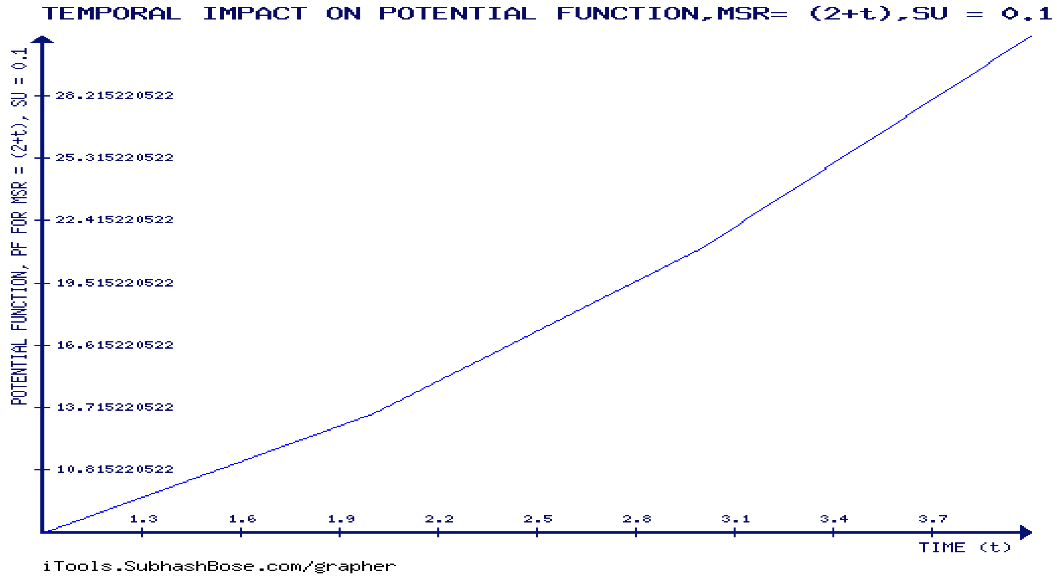
7.2. Numerical Experiments on the potential function, PF

In what follows,

S U = S e r v e r U t i l i z a t i o n = ρ, M S R = μ = M e a n S e r v i c e R a t e

t = t i m e, P F = P o t e n t i a l F u n c t i o n = Ψ (θ)

7.3. Numerical Experiments on the potential function, PF

In what follows,

S U = S e r v e r U t i l i z a t i o n = ρ, M S R = μ = M e a n S e r v i c e R a t e

t = t i m e, P F = P o t e n t i a l F u n c t i o n = Ψ (θ)

7.3.1. Numerical Experiment One

Ψ (θ) = - l n (ρ) - l n (1 - ρ) + μ (1 + ρ) t, μ = 2, t = 1

Figure 3.

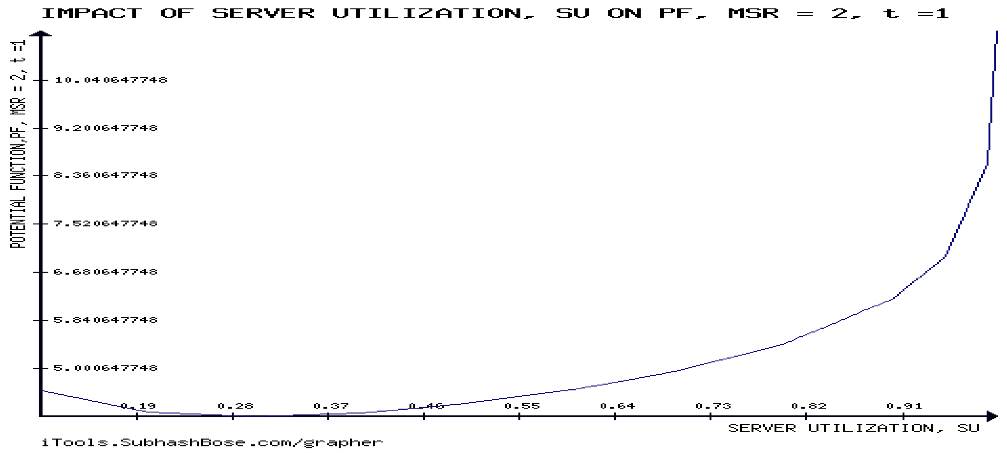
Figure 4.

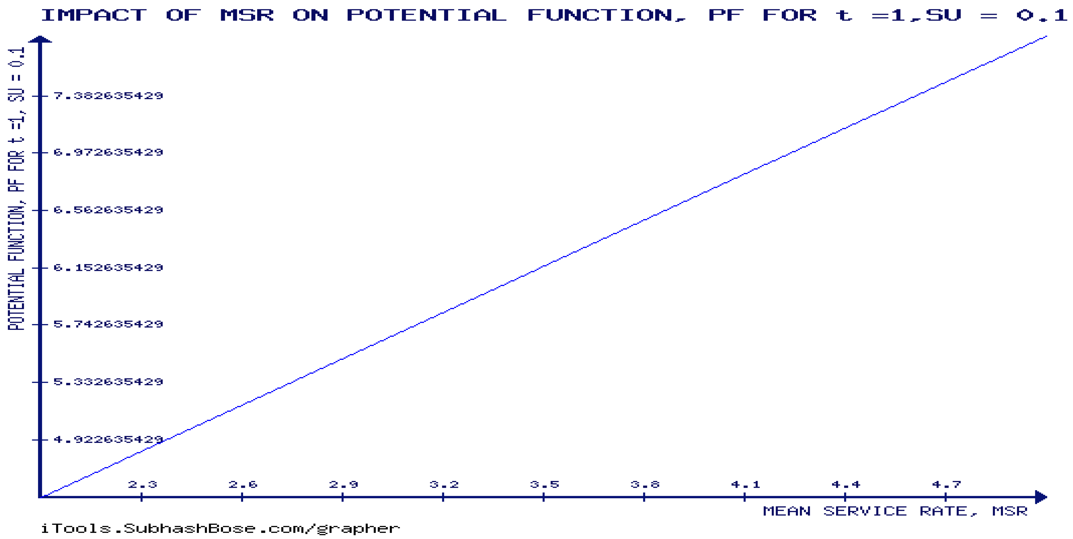
Communicating figure 3, the agreement of the experimental findings and the analytic results (c.f., (i) and (ii)of Theorem 7.1). The

ρ_{T h e s h o l d}

\frac{1 - 2 ρ}{2 ρ (1 - ρ)}

starts to be higher than the proposed temporal value,

t = 1

which enforces the decreasability of the potential function in server utilization. As the server utilization increases, the

ρ_{T h e s h o l d}

\frac{1 - 2 ρ}{2 ρ (1 - ρ)}

starts to be lower than the proposed temporal value,

t = 1

which enforces the increasability of the potential function in server utilization. This perfectly matches with the analytic results. Figure 4 shows that the potential function is forever increasing in mean service rate,

μ

. This matches with the analytic results.

More potentially,

\begin{matrix} Ψ (θ) = - l n (ρ) - l n (1 - ρ) + μ (1 + ρ) t, μ = 2 + t, ρ = 0.1 \\ = - l n (0.099) + (1.1) (2 + t) t, t_{T h e s h o l d} = \frac{ρ^{.} (\frac{1 - 2 ρ}{ρ (1 - ρ)}) - μ (1 + ρ)}{((1 + ρ) μ^{.} + μ ρ^{.})} = \frac{- (1.1) (t + 2)}{1.1} = - (t + 2) \end{matrix}

Figure 5.

As observed from figure 5 that the potential function is forever increasing in time, since time is greater than the calculated value of the

t_{T h e s h o l d}

. This shows that the experimental values agrtee with the obtained analytic results from Theorem 7.1.

9. SOME ALGEBRAIC PROPERTIES OF THE POTENTIAL FUNCTION, $Ψ (θ) = - l n (ρ) - l n (1 - ρ) + μ (1 + ρ) t ($ c.f., (3.20))

Theorem 4. The three-dimensional potential function

Ψ (θ) = - l n (ρ) - l n (1 - ρ) + μ (1 + ρ) t

(c.f., (34)) is generally not well-defined.

Proof. Let

ρ_{i}, μ_{i}, t_{i}

i = 1,2

be such that

ρ_{1} \neq ρ_{2},

μ_{1} \neq μ_{2}, t_{1} \neq t_{2} .

Let

Ψ (ρ_{1}, μ_{1}, t_{1}) = Ψ (ρ_{2}, μ_{2}, t_{2}) . T h i s i m p l i e s

- l n (ρ_{1}) - l n (1 - ρ_{1}) + μ_{1} (1 + ρ_{1}) t_{1} = - l n (ρ_{2}) - l n (1 - ρ_{2}) + μ_{2} (1 + ρ_{2}) t_{2}

(71)

(71)

directly implies:

l n (\frac{ρ_{2 (1 - ρ_{2})}}{ρ_{1} (1 - ρ_{1})}) = μ_{2} (1 + ρ_{2}) t_{2} - μ_{1} (1 + ρ_{1}) t_{1}

(72)

Assuming that

ρ_{1} = ρ_{2}

. This transforms (72) to

0 = (1 + ρ_{1}) [μ_{2} t_{1} - μ_{1} t_{1}]

(73)

Clearly (73) is satisfied if and only if

μ_{2} t_{1} = μ_{1} t_{1} (since (1 + ρ_{1}) \neq 0)

(74)

It can be verified that (74) is generated for values

μ_{1} \neq μ_{2}, t_{1} \neq t_{2},

which proves that

Ψ (θ)

is not well-defined in general.

Several emerging important special cases of Theorem 9.1 are obtained in the following theorems.

Theorem 2. For constant values of

μ, t

, the three-dimensional potential function

Ψ_{ρ} (θ) = - l n (ρ) - l n (1 - ρ) + μ (1 + ρ) t

(c.f., (34)) is not well-defined in general .

P r o o f .

For constant values of

μ, t, d e f i n e ρ_{i}, i = 1,2

be such that

ρ_{1} \neq ρ_{2} .

Thus,

Ψ (ρ_{1}, μ, t) = Ψ (ρ_{2}, μ, t)

implies:

- l n (ρ_{1}) - l n (1 - ρ_{1}) + μ (1 + ρ_{1}) t = - l n (ρ_{2}) - l n (1 - ρ_{2}) + μ (1 + ρ_{2}) t

(75)

Hence, it follows that

l n (\frac{ρ_{2} (1 - ρ_{2})}{ρ_{1} (1 - ρ_{1})}) = μ {t (ρ}_{2} - ρ_{1})

(76)

Consequently, it follows from (76) that

(\frac{ρ_{2} (1 - ρ_{2})}{ρ_{1} (1 - ρ_{1})}) = e^{μ {t (ρ}_{2} - ρ_{1})}

(77)

One of the infinitely many solutions of (77) is

ρ_{1} = ρ_{2}

. This means that

Ψ_{ρ}

is not generally well-defined.

Theorem 3. For constant

ρ

μ,

the potential function

Ψ_{t} (θ) = - l n (ρ) - l n (1 - ρ) + μ (1 + ρ) t

(c.f., (34)) satisfies the following:

(1) Ψ_{t} (θ)

is well-defined.

(2) Ψ_{t} (θ) i s

onto.

(3) Ψ_{t} (θ) i s o n e - t o - o n e .

(4)

Ψ_{t} (θ) h a s a u n i q u e i n v e r s e, Ψ_{t}^{- 1}

given by

Ψ_{t}^{- 1} (ρ, μ, t) = \frac{t + l n (ρ (1 - ρ))}{μ (1 + ρ)}

(78)

P r o o f .

(1)For constant

ρ, μ

and

t_{1} \neq t_{2}

, let

- l n (ρ) - l n (1 - ρ) + μ (1 + ρ) t_{1} = - l n (ρ) - l n (1 - ρ) + μ (1 + ρ) t_{2}

(79)

This implies

μ (1 + ρ) t_{1} = μ (1 + ρ) t_{2}

(80)

Clearly, (81) implies:

μ (1 + ρ) (t_{1} - t_{2}) = 0

(81)

(82)

holds if and only if

μ = 0 (i m p o s s i b l e, s i n c e μ > 1) o r (1 + ρ) = 0 (i m p o s s i b l e s i n c e ρ \in (0,1)) o r

t_{1} - t_{2} = 0 w h i c h i m p l i e s t h a t t_{1} = t_{2}

. Hence, the proof of (1) follows.

(2) It is clear that for every

- l n (ρ) - l n (1 - ρ) + μ (1 + ρ) t,

There is a unique triad (

ρ, μ, t

) such that

ψ (ρ, μ, t) = - l n (ρ) - l n (1 - ρ) + μ (1 + ρ) t

(82)

T h i s p r o v e s (2) .

To prove (3), we need to show that

(ρ, μ, t_{1}) = ψ (ρ, μ, t_{2}) if and only if t_{1} = t_{2}

(83)

T h e p r o o f o f (9.12) i s s t r a i g h t f o r w a r d .

To prove (4), let

ψ (ρ, μ, t) = - l n (ρ) - l n (1 - ρ) + μ (1 + ρ) t = y . T h i s i m p l i e s t h a t

t = \frac{y + l n (ρ (1 - ρ))}{μ (1 + ρ)}

, which directly implies

Ψ_{t}^{- 1} (ρ, μ, t) = \frac{t + l n (ρ (1 - ρ))}{μ (1 + ρ)}

Theorem 4. For constant

ρ

t,

the potential function

Ψ_{μ} (θ) = - l n (ρ) - l n (1 - ρ) + μ (1 + ρ) t

(c.f., (34)) satisfies the following:

(1) Ψ_{μ} (θ)

is well-defined.

(2) Ψ_{μ} (θ) i s

onto.

(3) Ψ_{μ} (θ) i s o n e - t o - o n e .

(4)

Ψ_{μ} (θ) h a s a u n i q u e i n v e r s e, Ψ_{μ}^{- 1}

given by

Ψ_{μ}^{- 1} (ρ, μ, t) = \frac{μ + l n (ρ (1 - ρ))}{t (1 + ρ)}

(84)

P r o o f .

The proofs are similar to Theorem 9.4.

10. The Threshold Theorems Of The Derived Inverses Of Poten-Tial Function, Ipfs

Theorem 10.1 For the inverse potential function,

Ψ_{t}^{- 1} (ρ, μ, t) = \frac{t + l n (ρ (1 - ρ))}{μ (1 + ρ)}

(85)

The following hold

Ψ_{t}^{- 1} (ρ, μ, t)

is forever increasing in

t

ii)

Ψ_{t}^{- 1} (ρ, μ, t)

is never decreasing in

t

iii)

Ψ_{t}^{- 1} (ρ, μ, t)

is forever increasing in

μ

if and only if

t < l n (\frac{1}{ρ (1 - ρ)})

(86)

iv)

Ψ_{t}^{- 1} (ρ, μ, t)

is forever decreasing in

μ

if and only if

t > l n (\frac{1}{ρ (1 - ρ)})

(87)

Ψ_{t}^{- 1} (ρ, μ, t)

is forever increasing in

ρ

if and only if

t < [\frac{1 - ρ - 2 ρ^{2}}{ρ (1 - ρ)} + l n (\frac{1}{ρ (1 - ρ)})]

(88)

vi)

Ψ_{t}^{- 1} (ρ, μ, t)

is forever decreasing in

ρ

if and only if

t > [\frac{1 - ρ - 2 ρ^{2}}{ρ (1 - ρ)} + l n (\frac{1}{ρ (1 - ρ)})]

(89)

Proof.

i) We have

\frac{{\partial Ψ}_{t}^{- 1}}{\partial t} = \frac{1}{μ (1 + ρ)}

(90)

B y t h e p r e l i m i n a r y t h e o r e m, Ψ_{t}^{- 1}

is forever increasing since

μ > 1, ρ \in (0,1)

. Following (10.5), it is implied that i) holds.

T h e p r o o f o f i i) i s i m m e d i a t e b y (10.5) .

i i i) I t c a n b e s h o w n t h a t

\frac{{\partial Ψ}_{t}^{- 1}}{\partial μ} = - \frac{t + l n (ρ (1 - ρ))}{μ^{2} (1 + ρ)}

(91)

Engaging the same approach,

\frac{{\partial Ψ}_{t}^{- 1}}{\partial μ} > 0

if and only if

t + l n (ρ (1 - ρ)) < 0

(92)

(92) holds if and only if

< - l n (ρ (1 - ρ))

(93)

H e n c e, i i i) f o l l o w s .

F o l l o w i n g t h e s a m e a p p r o a c h, i v) h o l d s .

v) We have

\frac{{\partial Ψ}_{t}^{- 1}}{\partial ρ} = \frac{1}{μ} [\frac{(1 - ρ - 2 ρ^{2}) - ρ (1 - ρ) (t + l n (ρ (1 - ρ)))}{ρ (1 - ρ) {(1 + ρ)}^{2}}]

(94)

Engaging the same approach,

\frac{{\partial Ψ}_{t}^{- 1}}{\partial ρ} > 0

if and only if

(1 - ρ - 2 ρ^{2}) - ρ (1 - ρ) (t + l n (ρ (1 - ρ))) > 0

(95)

Clearly, by (95) and the Preliminary Theorem (PT), v) holds.

A similar approach proves vi).

Theorem 5. For the inverse potential function,

Ψ_{μ}^{- 1} (ρ, μ, t) = \frac{μ + l n (ρ (1 - ρ))}{t (1 + ρ)}

The following hold

Ψ_{μ}^{- 1} (ρ, μ, t)

is forever decreasing in

t

ii)

Ψ_{μ}^{- 1} (ρ, μ, t)

is never increasing in

t

iii)

Ψ_{μ}^{- 1} (ρ, μ, t)

is forever increasing in

μ

iv)

Ψ_{μ}^{- 1} (ρ, μ, t)

is never decreasing in

μ

Ψ_{μ}^{- 1} (ρ, μ, t)

is forever increasing in

ρ

if and only if

μ < [\frac{1 - ρ - 2 ρ^{2}}{ρ (1 - ρ)} + l n (\frac{1}{ρ (1 - ρ)})]

(96)

vi)

Ψ_{t}^{- 1} (ρ, μ, t)

is forever decreasing in

ρ

if and only if

μ > [\frac{1 - ρ - 2 ρ^{2}}{ρ (1 - ρ)} + l n (\frac{1}{ρ (1 - ρ)})]

(97)

Proof.

The proofs are analogous to Theorem 10.1.

11. NUMERICAL EXPERIMENTS ON THE THRESHOLD THEOREMS OF THE DERIVED INVERSES OF POTENTIAL FUNCTION

11.1. Numerical Experiment on Theorem 11.1

We have, the inverse of the potential function, IPF=

Ψ_{t}^{- 1} (ρ, μ, t) = \frac{t + l n (ρ (1 - ρ))}{μ (1 + ρ)} (c . f .,

(85)).

Theorem 6. For the inverse potential function,

Ψ_{t}^{- 1} (ρ, μ, t) = \frac{t + l n (ρ (1 - ρ))}{μ (1 + ρ)}

The following hold

Ψ_{t}^{- 1} (ρ, μ, t)

is forever increasing in

t

ii)

Ψ_{t}^{- 1} (ρ, μ, t)

is never decreasing in

t

iii)

Ψ_{t}^{- 1} (ρ, μ, t)

is forever increasing in

μ

if and only if

t < l n (\frac{1}{ρ (1 - ρ)})

(98)

iv)

Ψ_{t}^{- 1} (ρ, μ, t)

is forever decreasing in

μ

if and only if

t > l n (\frac{1}{ρ (1 - ρ)})

(99)

Ψ_{t}^{- 1} (ρ, μ, t)

is forever increasing in

ρ

if and only if

t < [\frac{1 - ρ - 2 ρ^{2}}{ρ (1 - ρ)} + l n (\frac{1}{ρ (1 - ρ)})]

(100)

vi)

Ψ_{t}^{- 1} (ρ, μ, t)

is forever decreasing in

ρ

if and only if

t > [\frac{1 - ρ - 2 ρ^{2}}{ρ (1 - ρ)} + l n (\frac{1}{ρ (1 - ρ)})]

(101)

It can be seen that the temporal performance behaviour,

Ψ_{t}^{- 1} (ρ, μ, t) = \frac{t + l n (ρ (1 - ρ))}{μ (1 + ρ)}

Figure 6.

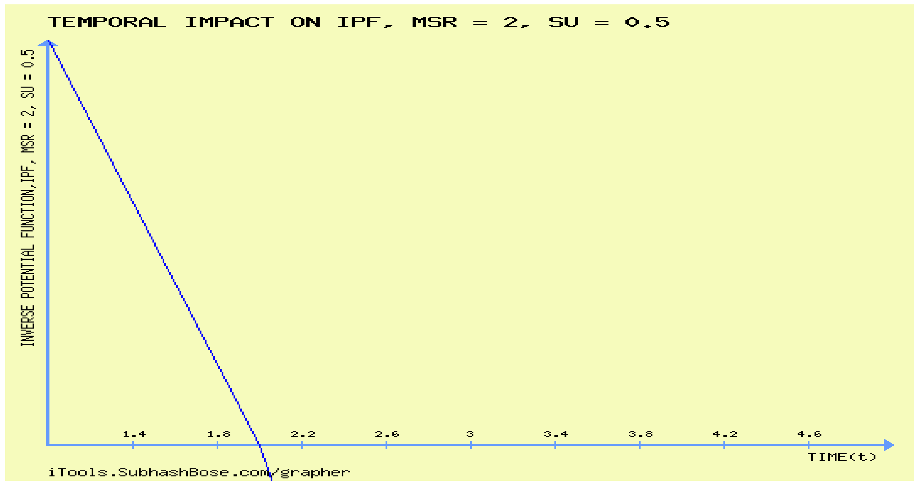
It is observed from figure 6 that

Ψ_{t}^{- 1} (ρ, μ, t)

is forever decreasing in time and never increase in time.

As for the performance behaviour in Mean service Time,

Let

t = 1, ρ = 0.5,

l n (\frac{1}{ρ (1 - ρ)}) = 1.386294361 > 1 = t

Figure 7.

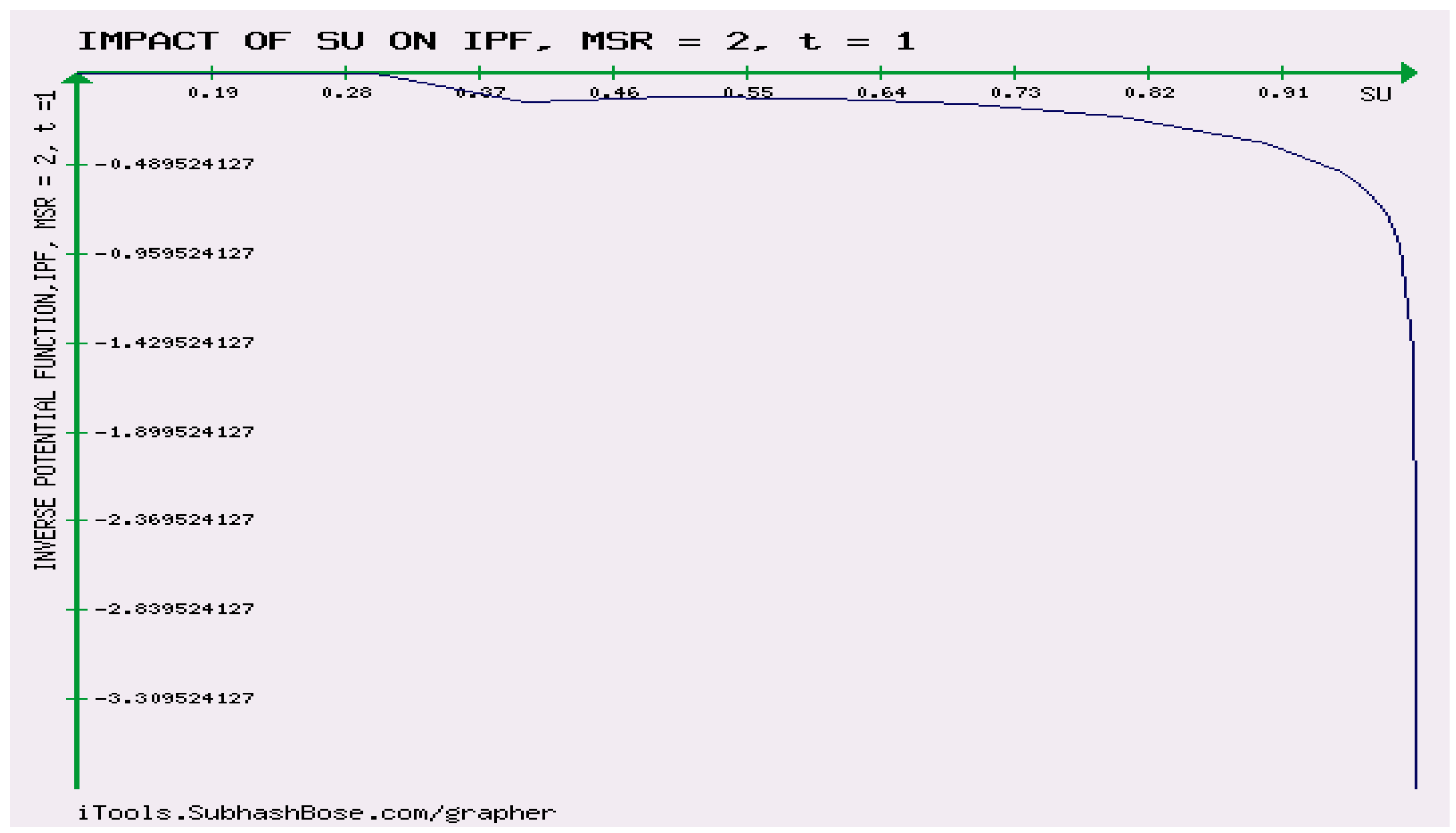
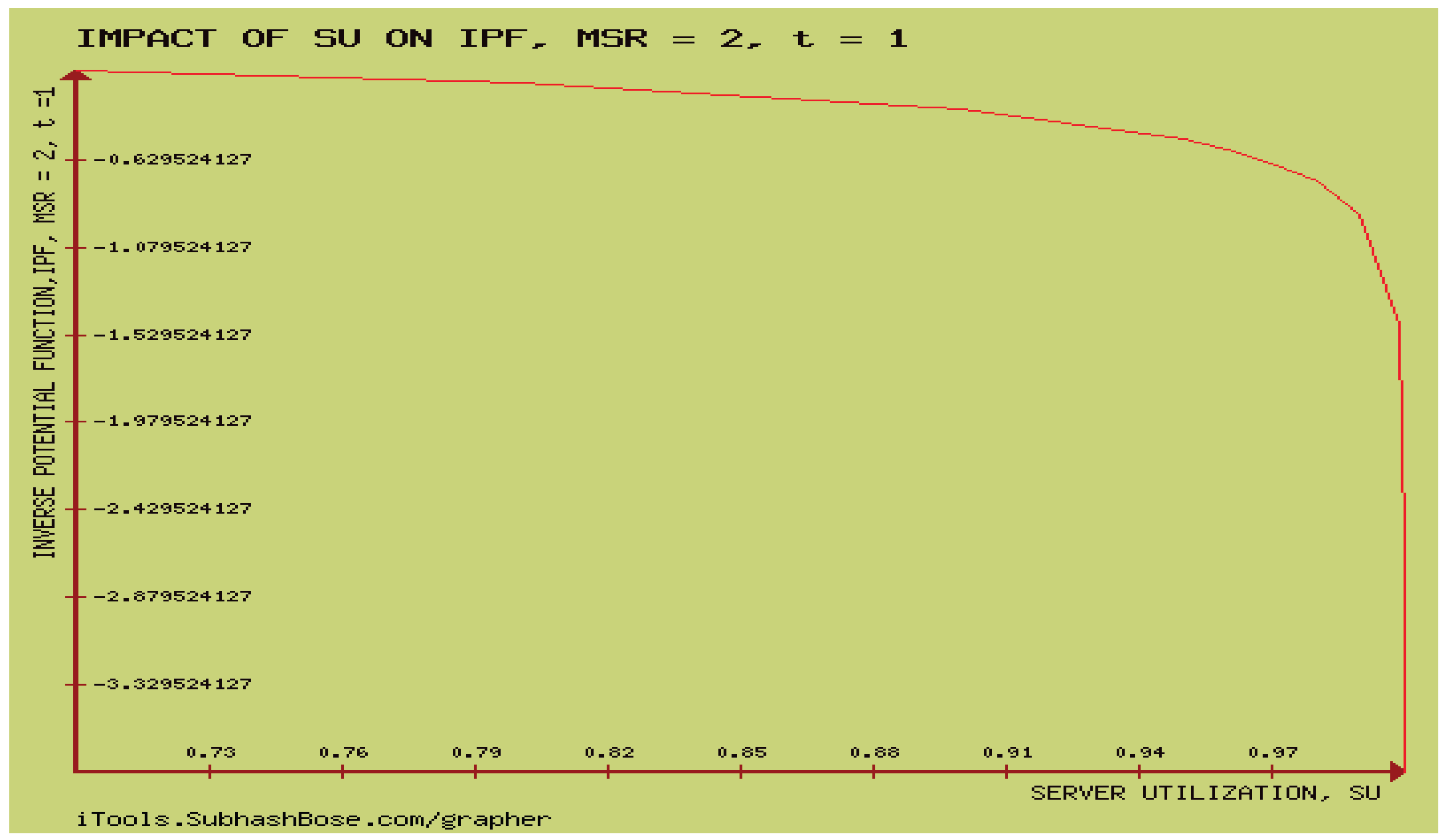
It is observed from figure 10 that as time is lower than

ρ_{T h r e s h o l d} = [\frac{1 - ρ - 2 ρ^{2}}{ρ (1 - ρ)} + l n (\frac{1}{ρ (1 - ρ)})]

Ψ_{t}^{- 1} (ρ, μ, t) = \frac{t + l n (ρ (1 - ρ))}{μ (1 + ρ)}

increases with respect to server utilization until times becomes greater than

ρ_{T h r e s h o l d},

the inverse potential function starts to decrease against the increase of server utilization. This shows that the numerical results numerically match the analytical results of v) and vi) Theorem 10.1. To make this clearer, the reader is advised to look at figures 7-10.

Figure 8.

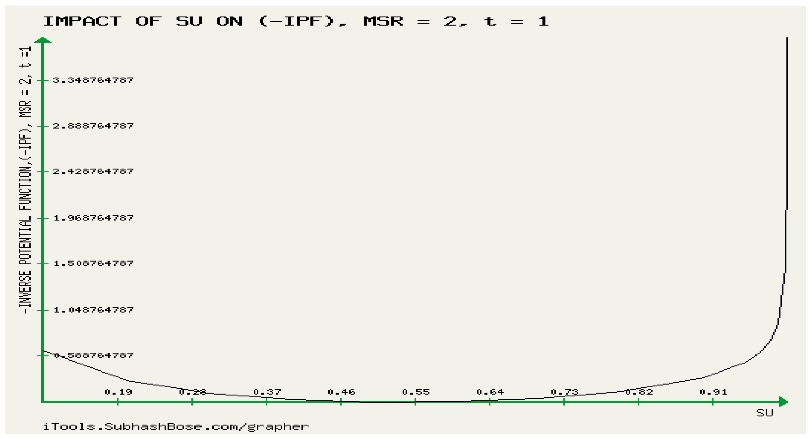
Figure 9.

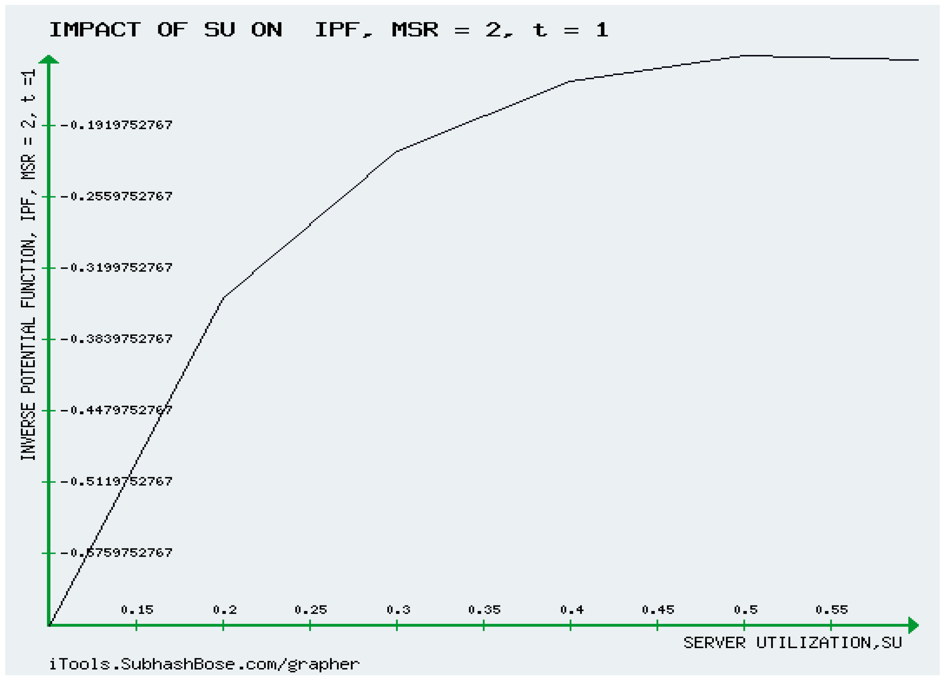
Figure 10.

12. THE $α -$ GAUSSIAN CURVATURE, $K_{0}^{(α)}$ OF (2.14) AS TIME APPROACHES INFINITY

Theorem 12.1 The

α -

Gaussian Curvature,

K_{0}^{(α)}

as time approaches zero is devised by

K_{0}^{(α)} = [\frac{(1 - α) [\frac{1}{ρ^{2}} - \frac{1}{{(1 - ρ)}^{2}}] ρ^{.}}{2 {(1 + ρ)}^{3}}]

(102)

Proof.

We have

\begin{matrix} {\begin{matrix} R \end{matrix}}_{i j k l}^{(α)} = [(\partial_{j} Γ_{i k}^{s (α)} - \partial_{i} Γ_{j k}^{s (α)}) g_{s l} + (Γ_{j β, l}^{(α)} Γ_{i k}^{β (α)} - \\ Γ_{i β, l}^{(α)} Γ_{j k}^{β (α)})] \end{matrix}

where

Γ_{i j}^{k (α)} = Γ_{i j, s}^{(α)} g^{s k}

, i,j,k,s = 1,2,...,n

Therefore,

R_{1212}^{(α)} = [(\partial_{2} Γ_{11}^{s (α)} - \partial_{1} Γ_{21}^{s (α)}) g_{s l} + (Γ_{j β, l}^{(α)} Γ_{11}^{β (α)} - Γ_{i β, l}^{(α)} Γ_{21}^{β (α)})] = [\begin{matrix} (\frac{\partial}{\partial μ} {[Γ}_{11}^{1 (α)} + Γ_{11}^{2 (α)} + Γ_{11}^{3 (α)}] - \frac{\partial}{\partial ρ} {[Γ}_{21}^{1 (α)} + Γ_{21}^{2 (α)} + Γ_{21}^{3 (α)}]) {(g}_{12} + g_{22} + g_{32}) \\ + ([Γ_{21,2}^{(α)} Γ_{11}^{1 (α)} + Γ_{22,2}^{(α)} Γ_{11}^{2 (α)} + Γ_{23,2}^{(α)} Γ_{11}^{3 (α)}] - {[Γ}_{11,2}^{(α)} Γ_{21}^{1 (α)} + Γ_{12,2}^{(α)} Γ_{21}^{2 (α)} + Γ_{13,2}^{(α)} Γ_{21}^{3 (α)}]) \end{matrix}] = [\begin{matrix} (\begin{matrix} \frac{\partial}{\partial μ} [(1 - α) ρ^{.} L (\frac{1}{{(1 - ρ)}^{3}} - \frac{1}{ρ^{3}}) + (1 - α) ρ^{.} (\frac{1}{{(1 - ρ)}^{3}} - \frac{1}{ρ^{3}}) F + (1 - α) ρ^{.} (\frac{1}{{(1 - ρ)}^{3}} - \frac{1}{ρ^{3}}) H] \\ - \frac{\partial}{\partial ρ} [\frac{(1 - α) L ρ^{.}}{2} + \frac{(1 - α) F ρ^{.}}{2} + \frac{(1 - α) H ρ^{.}}{2}] \end{matrix}) {(g}_{12} + g_{22} + g_{32}) \\ + (- [\frac{(1 - α)}{2} \frac{(1 - α) H ρ^{.}}{2}]) \end{matrix}]

(103)

Recall that

L = \frac{(b h)}{∆} = \frac{t [(1 + ρ) + t ρ^{.}]}{∆}

F = \frac{(b c - a h)}{∆} = \frac{(t [\frac{ρ^{.}}{ρ^{2}} + \frac{ρ^{.}}{{(1 - ρ)}^{2}} + t μ^{.} + μ ρ^{.}] - [\frac{1}{ρ^{2}} - \frac{1}{{(1 - ρ)}^{2}}] [(1 + ρ) + t ρ^{.}]}{∆}

H = \frac{(- b^{2})}{∆} = \frac{- t^{2}}{∆}

Where

R_{1212}^{(α)} ∆ = ([\frac{1}{ρ^{2}} - \frac{1}{{(1 - ρ)}^{2}}] (- {[(1 + ρ) + t ρ^{.}]}^{2}) - t (t (\frac{ρ^{. 2} - ρ ρ^{. .}}{ρ^{2}} + \frac{ρ^{. 2} + (1 - ρ) ρ^{. .}}{{(1 - ρ)}^{2}} + ((1 + ρ) t μ^{. .} + μ + {2 ρ}^{.} μ^{.} + 2 μ ρ^{.} + 2 ρ μ^{.} + μ t ρ^{. .}) - [\frac{ρ^{.}}{ρ^{2}} + \frac{ρ^{.}}{{(1 - ρ)}^{2}} + t μ^{.} + μ ρ^{.}] [(1 + ρ) + t ρ^{.}]) + [\frac{ρ^{.}}{ρ^{2}} + \frac{ρ^{.}}{{(1 - ρ)}^{2}} + t μ^{.} + μ ρ^{.}] (t [(1 + ρ) + t ρ^{.}]))

(104)

It could be verified that:

R_{1212}^{(α)} L_{t \to 0} = 0 = H_{t \to 0}, F_{t \to 0} = \frac{1}{(1 + ρ)}

(105)

Hence, it follows that:

R_{1212, t \to 0}^{(α)} = [\begin{matrix} (\begin{matrix} \frac{\partial}{\partial μ} [(1 - α) ρ^{.} L (\frac{1}{{(1 - ρ)}^{3}} - \frac{1}{ρ^{3}}) + (1 - α) ρ^{.} (\frac{1}{{(1 - ρ)}^{3}} - \frac{1}{ρ^{3}}) F + (1 - α) ρ^{.} (\frac{1}{{(1 - ρ)}^{3}} - \frac{1}{ρ^{3}}) H] \\ - \frac{\partial}{\partial ρ} [\frac{(1 - α) L ρ^{.}}{2} + \frac{(1 - α) F ρ^{.}}{2} + \frac{(1 - α) H ρ^{.}}{2}] \end{matrix}) ((1 + ρ) + t {(1 + ρ}^{.})) \\ + (- [\frac{(1 - α)}{2} \frac{(1 - α) H ρ^{.}}{2}]) \end{matrix}] \frac{(1 - α) ρ^{.}}{2 (1 + ρ)}

(106)

Clearly, it follows from the definition that

K_{t \to 0}^{(α)} = \frac{R_{1212, t \to 0}^{(α)}}{∆_{t \to 0}} = \frac{(1 - α) [\frac{1}{ρ^{2}} - \frac{1}{{(1 - ρ)}^{2}}] ρ^{.}}{2 {(1 + ρ)}^{3}}

(107)

In the following theorem, the zeros of the

α -

Gaussian Curvature

K_{0}^{(α)}

(c.f., (107)) are determined. Based on this, the paths of motion of the coordinates at which the underlying QM is looked at as a developable surface are obtained. The following theorem presents a novel approach which unifies Information Geometry with Riemannian Geometry, the theory of developable surfaces and the theory of time -dependent queueing systems.

Theorem 10. The

u n d e r l y i n g

M/M/

1

QM is developable on the following trajectories:

α = 1, or ρ = c o n s t a n t or ρ = \frac{1}{2} or ρ \to \infty (i n s t a b i l i t y p h a s e)

(108)

Proof.

K_{0}^{(α)} = 0 i f a n d o n l y i f

\frac{(1 - α) [\frac{1}{ρ^{2}} - \frac{1}{{(1 - ρ)}^{2}}] ρ^{.}}{2 {(1 + ρ)}^{3}} = 0

(109)

⟺ o n e o f w h a t f o l l o w s i s s a t i s f i e d

((1 - α) = 0 ⟹ α = 1

(110)

(1 - α) = 0 ⟹ α = 1

(111)

\frac{1}{ρ^{2}} - \frac{1}{{(1 - ρ)}^{2}} = 0 ⟹ {(1 - ρ)}^{2} = ρ^{2} ⟹ (1 - ρ) = \pm ρ ⟹ ρ = \frac{1}{2}, where 1 + ρ \neq 0 o r 1 = 0 (c o n t r a d i c t i o n)

(112)

(iv)

\frac{[1 - 2 ρ]}{{{(1 - ρ)}^{2} ρ^{2} (1 + ρ)}^{3}} = 0

. Let

ρ = \frac{1}{x}

, then

\frac{[x^{7} - 2 x^{6}]}{{{(x - 1)}^{2} (x + 1)}^{3}} = 0

which is equivalently,

x \to 0

, or

ρ \to \infty .

13. the $α - S e c t i o n a l$ Gaussian Curvatures of M/M/1 QM

R e c a l l t h a t

a = \frac{1}{ρ^{2}} - \frac{1}{{(1 - ρ)}^{2}}

(113)

b = t

(114)

c = \frac{ρ^{.}}{ρ^{2}} + \frac{ρ^{.}}{{(1 - ρ)}^{2}} + t μ^{.} + μ ρ^{.}

(115)

h = (1 + ρ) + t ρ^{.}

(116)

l = \frac{ρ^{. 2} - ρ ρ^{. .}}{ρ^{2}} + \frac{ρ^{. 2} + (1 - ρ) ρ^{. .}}{{(1 - ρ)}^{2}} + ((1 + ρ) t μ^{. .} + μ + {2 ρ}^{.} μ^{.} + 2 μ ρ^{.} + 2 ρ μ^{.} + μ t ρ^{. .}

(117)

Δ = d e t ([g_{i j}]) = (a (- h^{2}) - b (b l - c h) + c (b h))

We have

R_{1111, t \to 0}^{(α)} = [(\partial_{1} Γ_{11}^{s (α)} - \partial_{1} Γ_{11}^{s (α)}) g_{s 1} + (Γ_{1 β, 1}^{(α)} Γ_{11}^{β (α)} - Γ_{1 β, 1}^{(α)} Γ_{11}^{β (α)})] = 0

(118)

R_{1211}^{(α)} = [(\partial_{2} Γ_{11}^{s (α)} - \partial_{1} Γ_{21}^{s (α)}) g_{s 1} + (Γ_{2 β, l}^{(α)} Γ_{11}^{β (α)} - Γ_{1 β, l}^{(α)} Γ_{21}^{β (α)})]

(119)

Hence,

R_{1211, t \to 0}^{(α)} = [(\partial_{2} Γ_{11}^{s (α)} - \partial_{1} Γ_{21}^{s (α)}) g_{s 1} + (Γ_{2 β, l}^{(α)} Γ_{11}^{β (α)} - Γ_{1 β, l}^{(α)} Γ_{21}^{β (α)})] = [(\partial_{2} {(Γ}_{11}^{1 (α)} + Γ_{11}^{2 (α)} + Γ_{11}^{3 (α)}) - \partial_{1} {(Γ}_{21}^{1 (α)} + Γ_{21}^{2 (α)} + Γ_{21}^{3 (α)})) g_{s 1} + ([Γ_{21,1}^{(α)} Γ_{11}^{1 (α)} + Γ_{22,1}^{(α)} Γ_{11}^{2 (α)} + Γ_{23,1}^{(α)} Γ_{11}^{3 (α)}] - [Γ_{11,1}^{(α)} Γ_{21}^{1 (α)} + Γ_{12,1}^{(α)} Γ_{21}^{2 (α)} + Γ_{13,1}^{(α)} Γ_{21}^{3 (α)}])]

(120)

Δ = d e t ([g_{i j}]) = ([\frac{1}{ρ^{2}} - \frac{1}{{(1 - ρ)}^{2}}] (- {[(1 + ρ) + t ρ^{.}]}^{2}) - t (t [\frac{ρ^{. 2} - ρ ρ^{. .}}{ρ^{2}} + \frac{ρ^{. 2} + (1 - ρ) ρ^{. .}}{{(1 - ρ)}^{2}} + ((1 + ρ) t μ^{. .} + μ + {2 ρ}^{.} μ^{.} + 2 μ ρ^{.} + 2 ρ μ^{.} + μ t ρ^{. .}] - [\frac{ρ^{.}}{ρ^{2}} + \frac{ρ^{.}}{{(1 - ρ)}^{2}} + t μ^{.} + μ ρ^{.}] [(1 + ρ) + t ρ^{.}]) + [\frac{ρ^{.}}{ρ^{2}} + \frac{ρ^{.}}{{(1 - ρ)}^{2}} + t μ^{.} + μ ρ^{.}] (t [(1 + ρ) + t ρ^{.})]) ∆_{t \to 0} = - [\frac{1}{ρ^{2}} - \frac{1}{{(1 - ρ)}^{2}}] {(1 + ρ)}^{2} R_{1211, t \to 0}^{(α)} = = [\frac{(1 - α)}{2 {(1 + ρ)}^{2}} [\frac{1}{ρ^{2}} - \frac{1}{{(1 - ρ)}^{2}} + \frac{ρ^{.}}{ρ^{2}} + \frac{ρ^{.}}{{(1 - ρ)}^{2}} + μ ρ^{.}]

(121)

{T h e α - S e c t i o n a l c u r v a t u r e s, K}_{i j i j}^{(α)} = \frac{R_{i j i j}^{(α)}}{(g_{i i}) (g_{j j}) - {(g_{i j})}^{2}}

(c.f., Equation (8))

T h e α - S e c t i o n a l C u r v a t u r e s a s t i m e a p p r o a c h e s z e r o a r e g i v e n b y

K_{i j i j, t \to 0}^{(α)} = \frac{R_{i j i j, t \to 0}^{(α)}}{t \to 0}

(122)

T h e r e a d e r c a n e a s i l y c h e c k t h a t

K_{1111, t \to 0}^{(α)} = 0 = K_{1121, t \to 0}^{(α)} = K_{1113, t \to 0}^{(α)}

(123)

K_{1211, t \to 0}^{(α)} = \frac{R_{1211, t \to 0}^{(α)}}{Δ_{t \to 0}} = [\frac{(1 - α)}{2 {(1 + ρ)}^{2}} [\frac{1}{ρ^{2}} - \frac{1}{{(1 - ρ)}^{2}} + \frac{ρ^{.}}{ρ^{2}} + \frac{ρ^{.}}{{(1 - ρ)}^{2}} + μ ρ^{.}]

(124)

The remaining

α - S e c t i o n a l C u r v a t u r e s

can be obtained by following the same procedure.

14. Closing Remarks With Next Phase Research

This study offers a revolutionary info-geometrics of transient

M / M / 1

QM. For this queue, FIM and IFIM are established. The geodesic equations of motion for the queue's coordinates are established. More potentially, it is shown that the underlying queue has RCT

\neq 0

and a zero Gaussian curvature. The paper shows how Riemannian Geometric (RG) analysis, and the Theory of Relativity (TR) may be utilised to transient queues, providing a full analytical investigation and the potential for future applications to various queueing systems.

References

I. A. Mageed, Q. Zhang, T. C. Akinci, M. Yilmaz and M. S. Sidhu, "Towards Abel Prize: The Generalized Brownian Motion Manifold's Fisher Information Matrix With Info-Geometric Applications to Energy Works," 2022 Global Energy Conference (GEC), Batman, Turkey, 2022, pp. 379-384. [CrossRef]
Mageed IA, Yuyang Zhou, Y, Liu, Y, and Zhang Q, “ℤ_a,b of the Stable Five-Dimensional M/G/1 Queue Manifold Formalism’s Info- Geometric Structure with Potential Info-Geometric Applications to Human Computer Collaborations and Digital Twins”,In2023 28th International Conference on Automation and Computing (ICAC) 2023, 30^th Aug- Sep 1. IEEE. [CrossRef]
Mageed IA, Yuyang Zhou, Y, Liu, Y, and Zhang Q, “ Towards a Revolutionary Info-Geometric Control Theory with Potential Applications of Fokker Planck Kolmogorov(FPK) Equation to System Control, Modelling and Simulation”,In2023 28th International Conference on Automation and Computing (ICAC) 2023, 30^th Aug- Sep 1. IEEE. [CrossRef]
Mageed, I. A., & Zhang, K. Q. (2022). Information Geometry? Exercises de Styles. electronic Journal of Computer Science and Information Technology, 8(1), 9-14.
A Mageed, D.I. Info- Geometric Analysis of the Stable G/G/1 Queue Manifold Dynamics With G/G/1 Queue Applications to E-health. Preprints 2024, 2024011813. [CrossRef]
A Mageed, I. Info-Geometric Analysis of Human-Trust Based Feedback Control (HTBFC) Five-Dimensional Manifold with HTBFC Applications to Robotics. Preprints 2024, 2024012040. [CrossRef]
MIT Open Course Ware,2010. Online available at: https://ocw.mit.edu/courses/mathematics/18-02sc-multivariable-calculus-fall-2010/4.-triple-integrals-and-surface-integrals-in-3-space/part-b-flux-and-the-divergence-theorem/session-84-divergence-theorem/MIT18_02SC_MNotes_v10.1.pdf.
A Mageed, D.I. On the Kullback-Leibler Divergence Formalism (KLDF) of the Stable M/G/1 Queue Manifold, Its Information Geometric Structure and Its Matrix Exponential. Preprints 2024, 2024012092. [CrossRef]
Mageed, I. A., Kouvatsos, D.D., 2019, Information Geometric Structure of Stable M/G/1 Queue Manifold and its Matrix Exponential, Proceedings of the 35th UK Performance Engineering Workshop, School of Computing, University of Leeds, Edited by Karim Djemame, 16^th of Dec.2019, p.123-135. [Online] at: https://sites.google.com/view/ukpew2019/home.
Mageed, I.A, and Kouvatsos, D. (2021). The Impact of Information Geometry on the Analysis of the Stable M/G/1 Queue Manifold. In Proceedings of the 10th International Conference on Operations Research and Enterprise Systems - Volume 1: ICORES, ISBN 978-989-758-485-5, pages 153-160. [CrossRef]
A. Mageed, I. Towards An Info-Geometric Theory Of The Analysis Of Non-Time Dependent Queueing Systems. Preprints 2024, 2024012124. [CrossRef]
Weisstein, Eric W., 2021, Well-Defined, From MathWorld- A A Wolfram Web Resource. Available Online at: https://mathworld.wolfram.com/Well-Defined.html.
I. A. Mageed, "Fractal Dimension(D_f) Theory of Ismail’s Second Entropy(H_I^q) with Potential Fractal Applications to ChatGPT, Distributed Ledger Technologies(DLTs) and Image Processing(IP)," 2023 International Conference on Computer and Applications (ICCA), Cairo, Egypt, 2023, pp. 1-6. [CrossRef]
Mageed, I. A., & Zhang, Q. (2023). Threshold Theorems for the Tsallisian and Rényian (TR) Cumulative Distribution Functions (CDFs) of the Heavy-Tailed Stable M/G/1 Queue with Tsallisian and Rényian Entropic Applications to Satellite Images (SIs). electronic Journal of Computer Science and Information Technology, 9(1), 41-47.
I. A. Mageed, "Uniqeneness of The Time-Dependent Controller’s Designed Parameter (TDCDP) of Fokker Planck Kolmogorov(FPK) Probability Density Function(PDF) with Applications of Lambert W Function to Number Theory, Quantum Computing and Bitcoin Protocols," 2023 International Conference on Computer and Applications (ICCA), Cairo, Egypt, 2023, pp. 1-6. [CrossRef]
Kozma, L., 2020, Useful inequalities, online source. available at http://www.Lkozma.net/inequalities_cheat_sheet.
A Mageed, D.I. Upper and Lower Bounds of the State Variable of M/G/1 PSFFA Model of the Non-Stationary M/E_k/1 Queueing System. Preprints 2024, 2024012243. [CrossRef]
A Mageed, I. Info-Geometric Analysis of the Dynamics of Parthasarathian Transient Solution of M/M/1 Queue Manifold with Info-Geometric Applications to Machine Learning. Preprints 2024, 2024012008. [CrossRef]
Patil, D. P. (2021). Application of Sawi transform in Bessel functions. Aayushi International Interdisciplinary Research Journal (AIIRJ).

Disclaimer/Publisher’s Note: The statements, opinions and data contained in all publications are solely those of the individual author(s) and contributor(s) and not of MDPI and/or the editor(s). MDPI and/or the editor(s) disclaim responsibility for any injury to people or property resulting from any ideas, methods, instructions or products referred to in the content.

© 2024 by the authors. Licensee MDPI, Basel, Switzerland. This article is an open access article distributed under the terms and conditions of the Creative Commons Attribution (CC BY) license (http://creativecommons.org/licenses/by/4.0/).

Copyright: This open access article is published under a Creative Commons CC BY 4.0 license, which permit the free download, distribution, and reuse, provided that the author and preprint are cited in any reuse.

Downloads

Views

Comments

Subscription

Notify me about updates to this article or when a peer-reviewed version is published.

MDPI Initiatives

Important Links

Choose an area of interest and we will send you notifications of new preprints at your preferred frequency.

Disclaimer

On the Trio Unification of Information Geometry, Einsteinian Relativity, and Transient Queues the Parthasarathian Case

Abstract

Keywords:

Subject:

1. Introduction

2. Main Definitions

2.1. Main Definition on IG

2.2. Important Inequalities [16]

3. Fim and Ifim of the Transient M/M/1QM

4. Connection of the Transient M/M/1 QM

4.1. The Obtained Γ i j , k ( α ) Expressions (c.f., Equation (4)) of the Transient M/M/1 QM

5. THE IMEs OF THE COORDINATES THE TRANSIENT M/M/1 QM

5.1. The I M E s of the s e r v e r u t i l i z a t i o n coordinate, ρ of the transient M/M/1 QM

5.2. The I M E s of the M e a n s e r v i c e R a t e coordinate, μ of the transient M/M/1 QM

5.3. The I M E s of the t e m p o r a l coordinate, t of the transient M/M/1 QM

7. THE THRESHOLD THEOREMS FOR THE POTENTIAL FUNCTION OF EQUATION (34).

7.1. The Threshold Theorem for the Potential Function, TTPF (c.f., (34) of Theorem 3.1)

7.2. Numerical Experiments on the potential function, PF

7.3. Numerical Experiments on the potential function, PF

7.3.1. Numerical Experiment One

9. SOME ALGEBRAIC PROPERTIES OF THE POTENTIAL FUNCTION, Ψ θ = − l n ⁡ ρ − l n ⁡ 1 − ρ + μ 1 + ρ t ( c.f., (3.20))

10. The Threshold Theorems Of The Derived Inverses Of Poten-Tial Function, Ipfs

11. NUMERICAL EXPERIMENTS ON THE THRESHOLD THEOREMS OF THE DERIVED INVERSES OF POTENTIAL FUNCTION

11.1. Numerical Experiment on Theorem 11.1

12. THE α − GAUSSIAN CURVATURE, K 0 ( α ) OF (2.14) AS TIME APPROACHES INFINITY

13. the α − S e c t i o n a l Gaussian Curvatures of M/M/1 QM

14. Closing Remarks With Next Phase Research

References

MDPI Initiatives

Important Links

Subscribe

4.1. The Obtained $Γ_{i j, k}^{(α)}$ Expressions (c.f., Equation (4)) of the Transient M/M/1 QM

5.1. The $I M E s$ of the $s e r v e r u t i l i z a t i o n$ coordinate, $ρ$ of the transient M/M/1 QM

5.2. The $I M E s$ of the $M e a n s e r v i c e R a t e$ coordinate, $μ$ of the transient M/M/1 QM

5.3. The $I M E s$ of the $t e m p o r a l$ coordinate, $t$ of the transient M/M/1 QM

9. SOME ALGEBRAIC PROPERTIES OF THE POTENTIAL FUNCTION, $Ψ (θ) = - l n (ρ) - l n (1 - ρ) + μ (1 + ρ) t ($ c.f., (3.20))

12. THE $α -$ GAUSSIAN CURVATURE, $K_{0}^{(α)}$ OF (2.14) AS TIME APPROACHES INFINITY

13. the $α - S e c t i o n a l$ Gaussian Curvatures of M/M/1 QM