Submitted:
29 January 2024
Posted:
30 January 2024
You are already at the latest version
Abstract
A field sampling event was conducted to measure the concentrations of metals within the trunks of felled trees on a college campus east of New York City. Heavy metals, particularly chromium, were found present in the soils surrounding the sampled trees, allowing for a correlation coefficient to be calculated with soil and tree concentrations. A statistically significant Pearson correlation was found between these two concentrations among the samples. This study is aimed at providing researchers a starting point for their research a better understanding of local ecologies, prediction of future change, and dissemination of conservation efforts.
Keywords:
xrf
; dendrochemistry
; trees
; chromium
; metals
1. Introduction
X-ray fluorescence (XRF) is a non-destructive analytical technique used to determine the composition of materials. In XRF, an X-ray source is used to excite the inner-shell electrons of the atoms in the sample [1]. When these electrons drop back to their original energy levels, they emit secondary X-rays, which have a unique energy signature for each element [2]. These secondary X-rays can be detected by a detector, and the intensities of the various fluorescence lines are used to identify and quantify the elements present in the sample.
Dendrochemistry is the study of tree rings focusing on their chemical analysis to determine the environmental and biological factors that influence tree growth [3]. This field uses various analytical techniques to measure the concentration of chemical elements and compounds in tree rings, including XRF. By analyzing the chemical composition of tree rings, we can gain insights into the environmental conditions that trees have experienced during their growth, such as temperature, precipitation, soil nutrients, and atmospheric pollution. This information can be used to reconstruct past environmental conditions and study the effects of environmental changes on tree growth. Dendrochemical analysis can be used to monitor the health of trees and detect changes in the forest ecosystem that may indicate environmental stress.
Metals can enter tree rings through the process of uptake from the soil and/or the atmosphere. Trees absorb heavy metals and other pollutants through their roots and transport them to different parts of the plant, including the leaves, stems, and bark [4]. Over time, these pollutants become incorporated into the tree’s growth rings, which can provide a historical record of the levels of pollution in the environment. The exact mechanisms of how heavy metals enter trees depend on several factors, including the type of tree, the soil and atmospheric conditions, the source and extent of the pollution, and the age and growth rate of the tree [5]. In some cases, these elements may be absorbed from contaminated soil and groundwater, while in other cases it may enter the tree through the atmosphere through the process of foliar uptake [6].
When heavy metal-impacted wood is burned or incinerated, the metals can be released into the atmosphere in the form of fine particulate matter or gases [7]. This may pose a significant health risk to nearby populations, as inhaling metal-contaminated particulate matter can result in toxicity, particularly in children and pregnant women [8,9]. Lead toxicity, for instance, can cause a range of health effects, including damage to the nervous system, digestive problems, reproductive problems, and developmental delays [10,11,12,13]. Historical lead emission data is presented in Figure 1.
2. Literature Review
2.1. Bioindicators
Bioindicators are organisms, or a part of an organism, that provide information about the health and environmental conditions of an ecosystem [15]. Bioindicators are used to assess the impacts of environmental stressors such as pollutants, climate change, and habitat destruction [16]. They can also provide information about the presence of specific contaminants, such as heavy metals, in an ecosystem. Bioindicators can include plants, animals, and microorganisms, and can be used at the individual or population level.
Urban tree barks can be used as bioindicators of environmental pollution [17]. Bioindicators are organisms or tissues that can be used to assess environmental conditions, including pollution levels. Trees in an urban watershed had higher levels of trace elements (Cd, Cu, Pb, and Zn) compared to those in a nearby reference watershed [18]. A similar study demonstrated that concentrations of trace elements (Cu, Pb, and Ni) increased over the years, while the supply of nutrients decreased [19]. Lead has been documented to increase in concentration toward the outer tree rings, with up to a doubling of the concentration across this range [20].
2.2. Metals in the Environment
Heavy metals are naturally occurring elements that are present in the environment but can also be introduced through human activities such as mining, industrial processes, and the use of pesticides and fertilizers [21]. These elements can accumulate in plants and create negative effects on plant growth and health [22]. The prevalence of heavy metals in plants depends on a variety of factors, including the type of plant, the environment in which it grows, and the level of heavy metal contamination in the soil [5,23,24].
2.3. Electrons and X-Ray Generation
Electron excitation is the process by which an electron in an atom or molecule is raised to a higher energy level or excited state by gaining energy [25]. The energy can be gained through various mechanisms such as absorption of light or electromagnetic radiation, collision with another particle, or thermal energy. When an electron is excited, it moves from its ground state to an excited state, where it is found in a higher energy level [26]. This energy can be emitted again in the form of light or electromagnetic radiation, as the electron returns to its ground state. The energy, wavelength, and frequency of this emission can provide information about the chemical composition and properties of the material being studied [27].
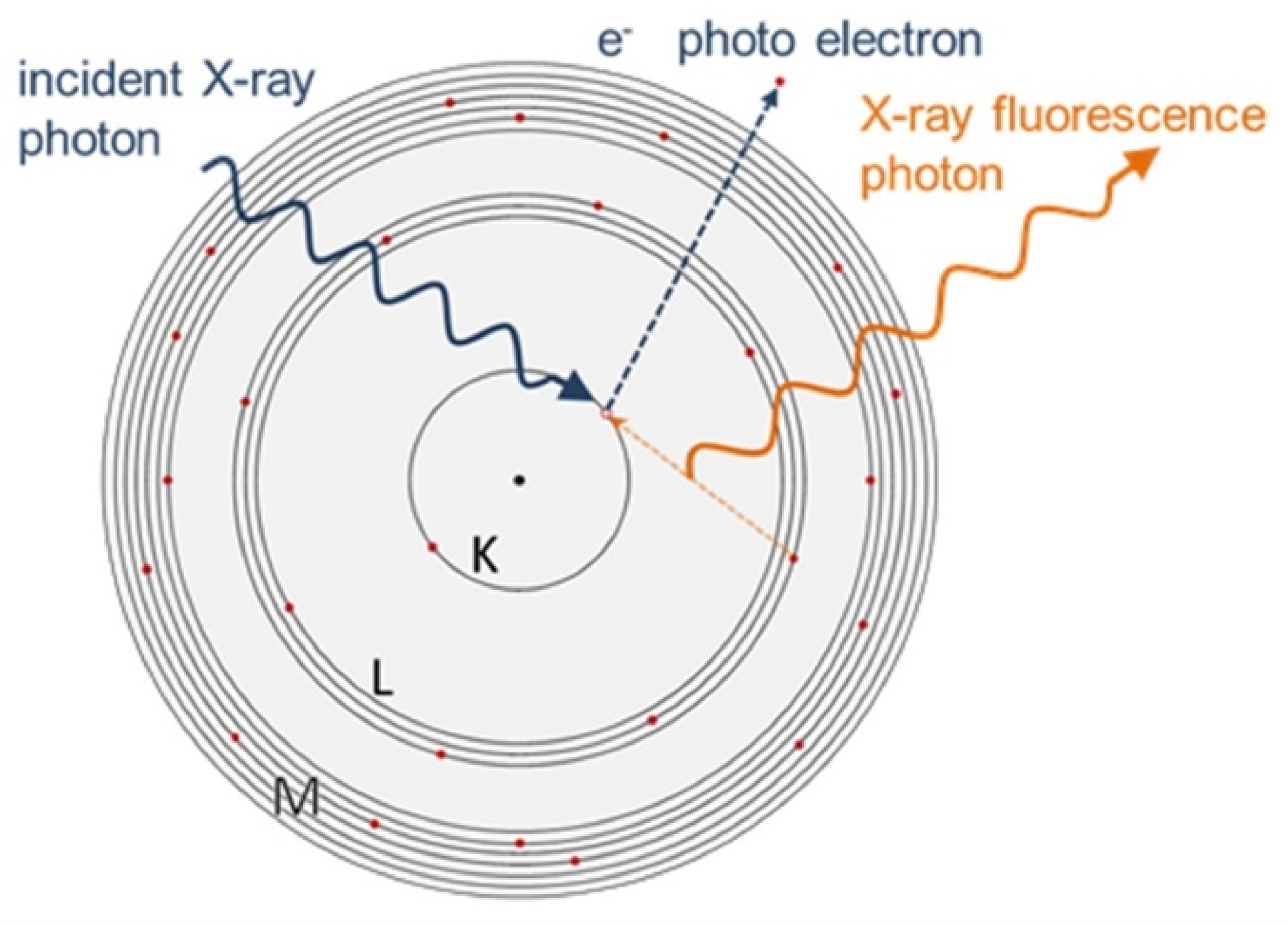
Figure 2.
XRF process [28].
Figure 2.
XRF process [28].
The phase setting is a critical parameter that determines the type and intensity of the X-ray radiation that is generated [29]. The phase setting determines the operating conditions of the XRF spectrometer, such as the voltage and current applied to the X-ray tube, and the configuration of the optics and detectors [30]. Different phase settings can be used to optimize the XRF measurement for different types of samples, sample matrices, and analytical goals. For example, a high voltage and high current setting may be used to generate high energy X-rays, while a low voltage and low current setting may be used to generate low energy X-rays [31]. The choice of phase setting is dependent on the energy and intensity of the X-rays that are required to excite the sample and generate the fluorescence X-rays, as well as the stability and repeatability of the measurement.
Changing the phase setting time can affect the count rate and intensity of the fluorescence signal [32]. A longer phase setting time will generally result in a higher count rate, but also increase the background noise, whereas a shorter phase setting time will result in a lower count rate, but also reduce the background noise [33]. The optimal phase setting time will depend on the specific sample, X-ray excitation source, and measurement conditions, and is often determined through trial and error, or through the use of a calibration sample.
3. Methodology
Taking an XRF sample is a multi-step process that involves preparing the sample, placing it in the XRF instrument, and analyzing the data. A general outline of the steps involved in taking include [34,35,36,37]:
- Sample preparation: Depending on the type of sample, it may need to be prepared in a specific way. For example, solid samples may need to be ground to a fine powder to ensure that the X-rays penetrate the entire sample (for destructive sampling). Liquid samples may be coated onto a solid substrate.
- Sample placement: A prepared sample is placed in an XRF instrument, or in a sample holder or on a sample stage for portable units. It is important to ensure that the sample is positioned correctly in or above the instrument to ensure accurate results.
- X-ray excitation: The XRF instrument uses an X-ray source to excite the inner-shell electrons of the atoms in the sample. When these electrons drop back to their original energy levels, they emit secondary X-rays that have a unique energy signature for each element.
- Data collection: The XRF instrument detects the secondary X-rays emitted from the sample and converts them into a spectrogram, which is a graphical representation of the fluorescence intensity as a function of energy. The spectrogram is analyzed to determine the composition of the sample.
- Data interpretation: The XRF data is interpreted to determine the elemental composition of the sample. This involves identifying the fluorescence lines in the spectrogram and comparing them to reference spectra for each element. The intensities of the fluorescence lines are used to quantitate the amount of each element present in the sample.
A Bruker S1 Titan Model 800 XRF was used to analyze sample data. This unit operates at four watts (4 W), with an excitation range up to 50 kilovolts. Its elemental range of analysis is from magnesium to uranium. The unit analyzed a calibration standard prior to sample analyses and was confirmed to be in proper operating condition. The phase setting time in an X-ray fluorescence (XRF) instrument refers to the duration during which the energy of the X-ray excitation source is kept at a specific level before the measurement is taken. This phase setting time is used to optimize the measurement conditions and can affect the accuracy and precision of the XRF analysis [28].
This study was used non-destructive sampling, so the portable XRF was held directly onto the tree stumps for the full length of the required time of ninety (90) seconds (3 phases at 30 seconds each). The Bruker S1 Titan stores data internally along with spectrograms, making interpretation simpler. The accuracy of the XRF results depends on several factors, including the quality of the sample preparation, the calibration of the XRF instrument, and the interpretation of the data. It is recommended to use standard reference materials to verify the accuracy of the XRF results.
Samples were chosen from felled trees in which the full trunk was exposed and had a minimum diameter of forty-five centimeters (45 cm). The physical location of the sampling event was in a wooded field in Nassau County, New York, United States adjacent to a relatively low-trafficked road. Samples were in the center of the tree trunk, its outer ring, and a point in the middle of those two (Figure 3. Nine (9) trees met the criteria for sampling. Ambient temperature was fourteen degrees (14 C).
The measurements recorded were with the XRF having its three phase settings each set to thirty seconds. Other phase timings were attempted and did not provide any significant variation for recording or analyzing the data.
4. Results
Data from the XRF was exported into a CSV file and then analyzed with R [38]. One sampled tree resulted in non-detectable chromium concentrations and was not used in calculations. The three chromium concentrations per tree were averaged and then plotted against the chromium concentration in the surrounding soil. There does appear to be a correlation between these two variables.
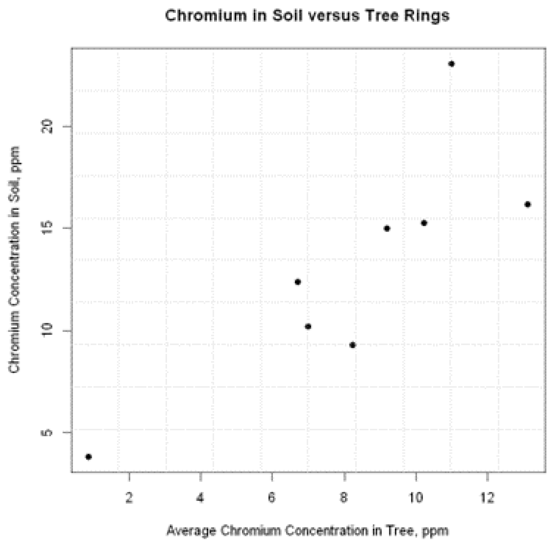
Figure 4.
Scatterplot of tree versus soil chromium concentrations.
A Pearson correlation was computed to assess the linear relationship between soil and average tree concentrations. There was a positive correlation between the two variables, r(6) = .832, p = .010. This represents a strong, positive correlation.
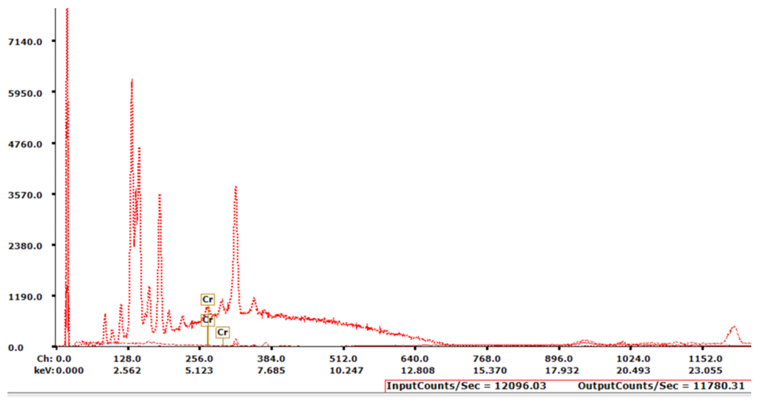
Peak identification from the XRF spectrum allows for the identification of any elements present in the sample. Each element has its own signature peak profile, so comparing the energy levels to known values can be accomplished. Software that accompanies this XRF unit does this automatically from a built-in database of known element spectra (Figure 5).
5. Discussion
There are some limitations of XRF scanners, including their sensitivity to surface effects and the need for careful sample preparation to ensure accurate results [1]. Conducting nondestructive in situ XRF analysis of tree samples may result in interference due to the presence of water [39]. Spectra may be flatter as the water molecules dilute the mass fraction of the analytes of interest.
In general, a longer XRF phase setting time can be used for samples with high fluorescence yield, whereas a shorter phase setting time is appropriate for samples with low fluorescence yield. By adjusting the phase setting time, it is possible to improve the sensitivity and accuracy of the XRF analysis [28,29,32].
6. Conclusions
XRF is widely used in a variety of fields, including geology, archaeology, metallurgy, environmental science, and many others. It is particularly useful for the analysis of samples that cannot be easily dissolved or that would be damaged by more aggressive analytical techniques [40]. Additionally, XRF is fast, efficient, and can be used to analyze large areas of a sample at once, making it a popular choice for both laboratory and field analysis.
Funding
This research received no external funding.
Data Availability Statement
Raw data can be made upon request from the author.
Conflicts of Interest
The authors declare no conflicts of interest.
References
- Croudace, I.W.; Löwemark, L.; Tjallingii, R.; Zolitschka, B. Current perspectives on the capabilities of high resolution XRF core scanners. Quaternary International 2019, 514, 5–15. [Google Scholar] [CrossRef]
- Singh, V.K.; Kawai, J.; Tripathi, D.K. (Eds.) X-ray fluorescence in biological sciences: principles, instrumentation and applications; Wiley: Hoboken, NJ, USA, 2022. [Google Scholar]
- Rocha, E.; Gunnarson, B.; Kylander, M.E.; Augustsson, A.; Rindby, A.; Holzkämper, S. Testing the applicability of dendrochemistry using X-ray fluorescence to trace environmental contamination at a glassworks site. Science of The Total Environment 2020, 720, 137429. [Google Scholar] [CrossRef]
- Edusei, G.; Tandoh, J.B.; Edziah, R.; Gyampo, O.; Ahiamadjie, H. Chronological Study of Metallic Pollution Using Tree Rings at Tema Industrial Area. Pollution 2021, 7. [Google Scholar] [CrossRef]
- Nawaz, R.; Aslam, M.; Nasim, I.; Irshad, M.A.; Ahmad, S.; Latif, M.; Hussain, F. Air Pollution Tolerance Index and Heavy Metals Accumulation of Tree Species for Sustainable Environmental Management in Megacity of Lahore. Air 2022, 1, 55–68. [Google Scholar] [CrossRef]
- Eichert, T.; Fernández, V. Uptake and release of elements by leaves and other aerial plant parts. In Marschner’s Mineral Nutrition of Plants; Elsevier, 2023; pp. 105–129. [Google Scholar] [CrossRef]
- Akbari, M.Z.; Thepnuan, D.; Wiriya, W.; Janta, R.; Punsompong, P.; Hemwan, P.; Charoenpanyanet, A.; Chantara, S. Emission factors of metals bound with PM2.5 and ashes from biomass burning simulated in an open-system combustion chamber for estimation of open burning emissions. Atmospheric Pollution Research 2021, 12, 13–24. [Google Scholar] [CrossRef]
- Sigsgaard, T.; Forsberg, B.; Annesi-Maesano, I.; Blomberg, A.; Bølling, A.; Boman, C.; Bønløkke, J.; Brauer, M.; Bruce, N.; Héroux, M.E.; Hirvonen, M.R.; Kelly, F.; Künzli, N.; Lundbäck, B.; Moshammer, H.; Noonan, C.; Pagels, J.; Sallsten, G.; Sculier, J.P.; Brunekreef, B. Health impacts of anthropogenic biomass burning in the developed world. European Respiratory Journal 2015, 46, 1577–1588. [Google Scholar] [CrossRef] [PubMed]
- Timonen, H.; Mylläri, F.; Simonen, P.; Aurela, M.; Maasikmets, M.; Bloss, M.; Kupri, H.L.; Vainumäe, K.; Lepistö, T.; Salo, L.; Niemelä, V.; Seppälä, S.; Jalava, P.; Teinemaa, E.; Saarikoski, S.; Rönkkö, T. Household solid waste combustion with wood increases particulate trace metal and lung deposited surface area emissions. Journal of Environmental Management 2021, 293, 112793. [Google Scholar] [CrossRef]
- Fu, Z.; Xi, S. The effects of heavy metals on human metabolism. Toxicology Mechanisms and Methods 2020, 30, 167–176. [Google Scholar] [CrossRef] [PubMed]
- Al osman, M.; Yang, F.; Massey, I.Y. Exposure routes and health effects of heavy metals on children. BioMetals 2019, 32, 563–573. [Google Scholar] [CrossRef]
- Naranjo, V.I.; Hendricks, M.; Jones, K.S. Lead Toxicity in Children: An Unremitting Public Health Problem. Pediatric Neurology 2020, 113, 51–55. [Google Scholar] [CrossRef]
- Levin, R.; Zilli Vieira, C.L.; Rosenbaum, M.H.; Bischoff, K.; Mordarski, D.C.; Brown, M.J. The urban lead (Pb) burden in humans, animals and the natural environment. Environmental Research 2021, 193, 110377. [Google Scholar] [CrossRef]
- Report on the Environment. Technical report, United States Environmental Protection Agency, 2018.
- Asif, N.; Malik, M.; Chaudhry, F. A Review of on Environmental Pollution Bioindicators. Pollution 2018, 4. [Google Scholar] [CrossRef]
- Salinitro, M.; Zappi, A.; Casolari, S.; Locatelli, M.; Tassoni, A.; Melucci, D. The Design of Experiment as a Tool to Model Plant Trace-Metal Bioindication Abilities. Molecules 2022, 27, 1844. [Google Scholar] [CrossRef]
- Caldana, C.R.; Hanai-Yoshida, V.M.; Paulino, T.H.; Baldo, D.A.; Freitas, N.P.; Aranha, N.; Vila, M.M.; Balcão, V.M.; Oliveira Junior, J.M. Evaluation of urban tree barks as bioindicators of environmental pollution using the X-ray fluorescence technique. Chemosphere 2023, 312, 137257. [Google Scholar] [CrossRef]
- Mazari, K.; Filippelli, G.M. Using deciduous trees as bioindicators of trace element deposition in a small urban watershed, Indianapolis, IN, USA. Journal of Environmental Quality 2020, 49, 163–171. [Google Scholar] [CrossRef]
- Świercz, A.; Świątek, B.; Pietrzykowski, M. Changes in the Concentrations of Trace Elements and Supply of Nutrients to Silver Fir (Abies alba Mill.) Needles as a Bioindicator of Industrial Pressure over the Past 30 Years in Świętokrzyski National Park (Southern Poland). Forests 2022, 13, 718. [Google Scholar] [CrossRef]
- Speer, J.H. Fundamentals of tree-ring research; University of Arizona Press: Tucson, 2020; OCLC: ocn460061751. [Google Scholar]
- Nazal, M.; Zhao, H. (Eds.) Heavy Metals - Their Environmental Impacts and Mitigation; IntechOpen: London, 2021. [Google Scholar]
- DalCorso, G.; Fasani, E.; Manara, A.; Visioli, G.; Furini, A. Heavy Metal Pollutions: State of the Art and Innovation in Phytoremediation. International Journal of Molecular Sciences 2019, 20, 3412. [Google Scholar] [CrossRef] [PubMed]
- Briffa, J.; Sinagra, E.; Blundell, R. Heavy metal pollution in the environment and their toxicological effects on humans. Heliyon 2020, 6, e04691. [Google Scholar] [CrossRef] [PubMed]
- Gautam, M.; Mishra, S.; Agrawal, M. Bioindicators of soil contaminated with organic and inorganic pollutants. In New Paradigms in Environmental Biomonitoring Using Plants; Elsevier, 2022; pp. 271–298. [Google Scholar] [CrossRef]
- Stevie, F.A.; Donley, C.L. Introduction to x-ray photoelectron spectroscopy. Journal of Vacuum Science & Technology A 2020, 38, 063204. [Google Scholar] [CrossRef]
- Brydson, R. Electron Energy Loss Spectroscopy, 1 ed.; Garland Science, 2020. [Google Scholar] [CrossRef]
- Greczynski, G.; Hultman, L. X-ray photoelectron spectroscopy: Towards reliable binding energy referencing. Progress in Materials Science 2020, 107, 100591. [Google Scholar] [CrossRef]
- S1 Titan/Tracer 5 User Manual, 2019.
- Declercq, Y.; Delbecque, N.; De Grave, J.; De Smedt, P.; Finke, P.; Mouazen, A.M.; Nawar, S.; Vandenberghe, D.; Van Meirvenne, M.; Verdoodt, A. A Comprehensive Study of Three Different Portable XRF Scanners to Assess the Soil Geochemistry of An Extensive Sample Dataset. Remote Sensing 2019, 11, 2490. [Google Scholar] [CrossRef]
- Beckhoff, B.; Beckhoff, B. Handbook of practical X-ray fluorescence analysis; Springer: Berlin New York, 2006. [Google Scholar]
- Haschke, M.; Flock, J.; Haller, M. X-ray Fluorescence Spectroscopy for Laboratory Applications; Wiley-VCH: Weinheim, Germany, 2021. [Google Scholar]
- Russ, J.C. Fundamentals of energy dispersive x-ray analysis. Butterworths monographs in materials, Butterworths: London, Boston, 2013. [Google Scholar]
- Fonseca, R. (Ed.) X-ray fluorescence: technology, performance and applications; Analytical chemistry and microchemistry, Nova Science Publishers, Incorporated: New York, 2018. [Google Scholar]
- Acquafredda, P. XRF technique. Physical Sciences Reviews 2019, 4. [Google Scholar] [CrossRef]
- Aylikci, N.K.; Oruc, O.; Bahceci, E.; Kahoul, A.; Depci, T.; Aylikci, V. Preparation of Sample for X-Ray Fluorescence Analysis. In X-Ray Fluorescence in Biological Sciences, 1 ed.; Singh, V.K., Kawai, J., Tripathi, D.K., Eds.; Wiley, 2022; pp. 91–113. [Google Scholar] [CrossRef]
- Byers, H.L.; McHenry, L.J.; Grundl, T.J. XRF techniques to quantify heavy metals in vegetables at low detection limits. Food Chemistry: X 2019, 1, 100001. [Google Scholar] [CrossRef]
- Croffie, M.E.T.; Williams, P.N.; Fenton, O.; Fenelon, A.; Metzger, K.; Daly, K. Optimising Sample Preparation and Calibrations in EDXRF for Quantitative Soil Analysis. Agronomy 2020, 10, 1309. [Google Scholar] [CrossRef]
- Team, R.C. R: A language and environment for statistical computing; R Foundation for Statistical Computing: Vienna, Austria, 2019. [Google Scholar]
- Gu, R.; Lei, M.; Chen, T.; Wan, X.; Dong, Z.; Wang, Y.; Qiao, P. Impact of Soil Water on the Spectral Characteristics and Accuracy of Energy-Dispersive X-ray Fluorescence Measurement. Analytical Chemistry 2019, 91, 5858–5865. [Google Scholar] [CrossRef]
- Singh, V.K.; Sharma, N.; Singh, V.K. Application of X-ray fluorescence spectrometry in plant science: Solutions, threats, and opportunities. X-Ray Spectrometry 2022, 51, 304–327. [Google Scholar] [CrossRef]
- Sánchez-Salguero, R.; Camarero, J.J.; Hevia, A.; Sangüesa-Barreda, G.; Galván, J.D.; Gutiérrez, E. Testing annual tree-ring chemistry by X-ray fluorescence for dendroclimatic studies in high-elevation forests from the Spanish Pyrenees. Quaternary International 2019, 514, 130–140. [Google Scholar] [CrossRef]
- Semeraro, T.; Luvisi, A.; De Bellis, L.; Aretano, R.; Sacchelli, S.; Chirici, G.; Marchetti, M.; Cocozza, C. Dendrochemistry: Ecosystem Services Perspectives for Urban Biomonitoring. Frontiers in Environmental Science 2020, 8, 558893. [Google Scholar] [CrossRef]
Figure 1.
Anthropogenic lead emissions in the United States by source category [14].
Figure 1.
Anthropogenic lead emissions in the United States by source category [14].
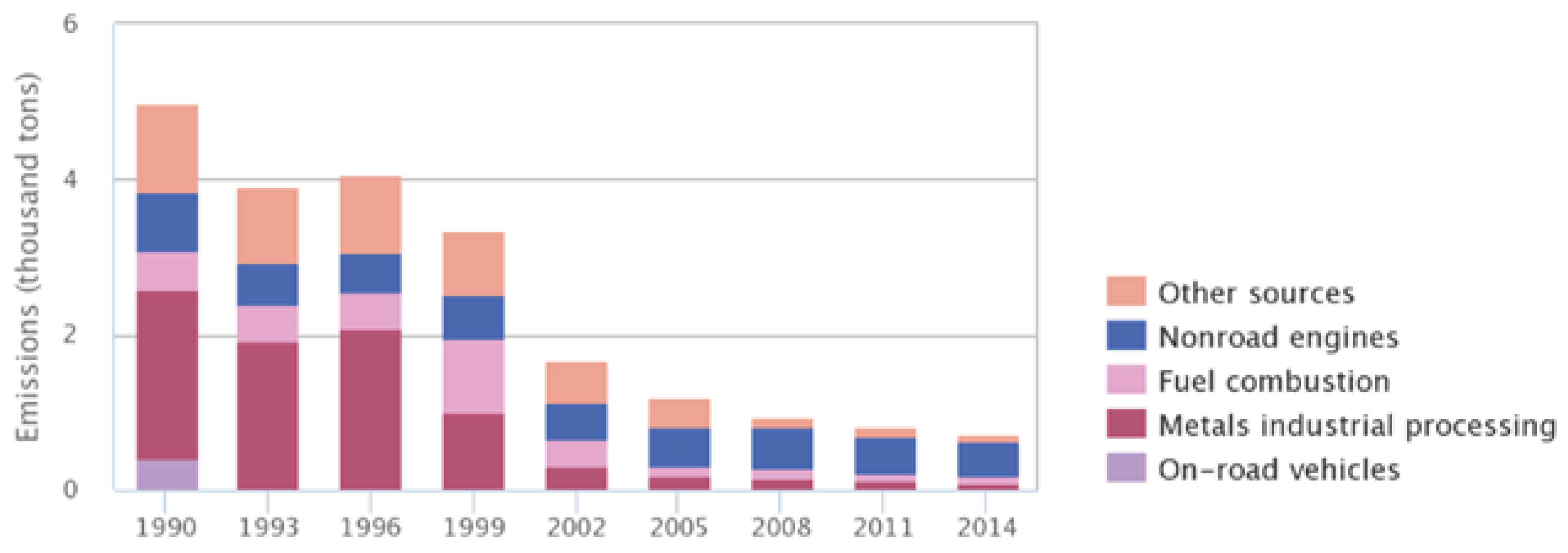
Figure 3.
Sampling locations (X) of tree stumps.
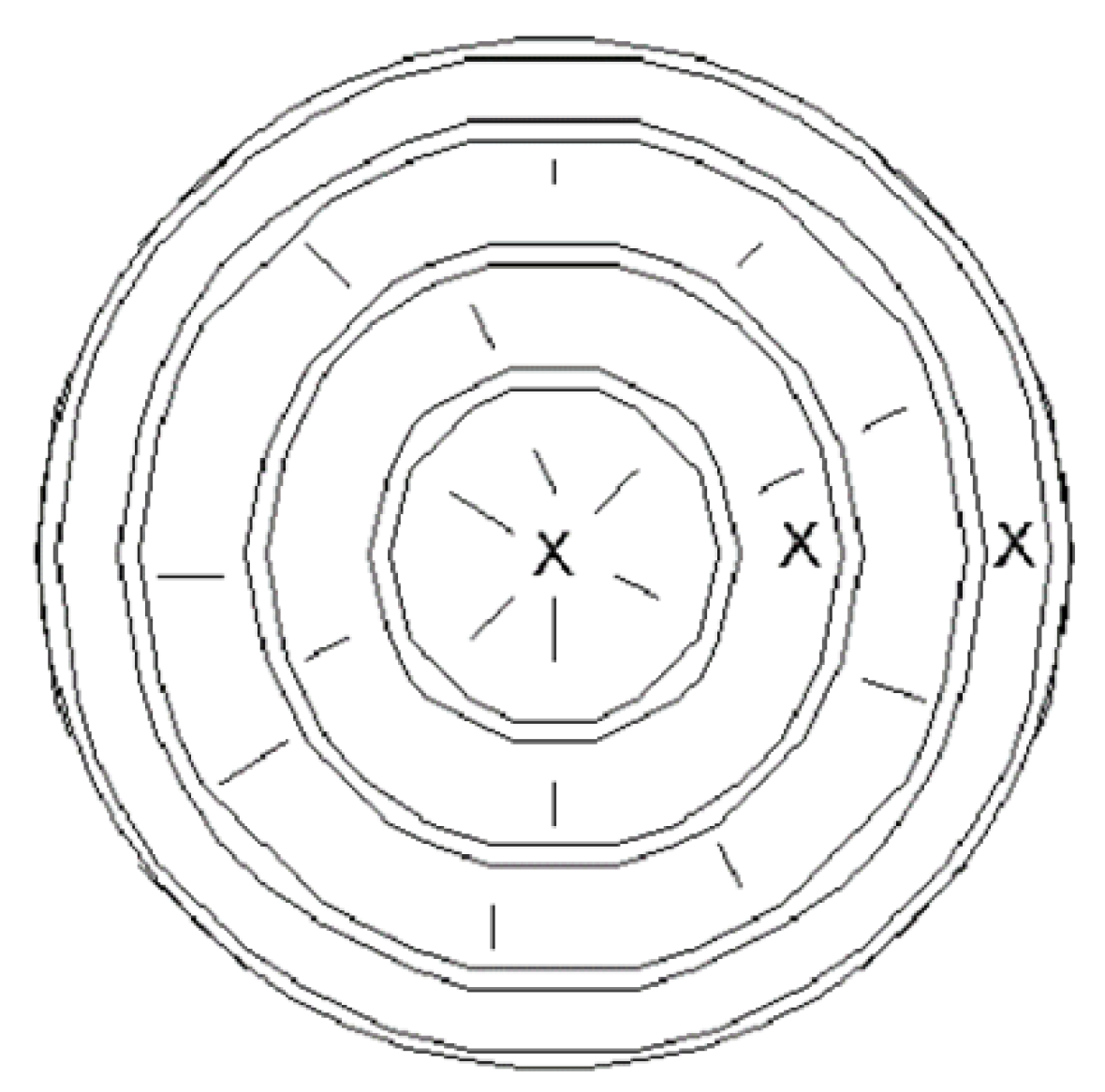
Figure 5.
Spectrum output for one observation.
Disclaimer/Publisher’s Note: The statements, opinions and data contained in all publications are solely those of the individual author(s) and contributor(s) and not of MDPI and/or the editor(s). MDPI and/or the editor(s) disclaim responsibility for any injury to people or property resulting from any ideas, methods, instructions or products referred to in the content. |
© 2024 by the authors. Licensee MDPI, Basel, Switzerland. This article is an open access article distributed under the terms and conditions of the Creative Commons Attribution (CC BY) license (http://creativecommons.org/licenses/by/4.0/).
Copyright: This open access article is published under a Creative Commons CC BY 4.0 license, which permit the free download, distribution, and reuse, provided that the author and preprint are cited in any reuse.


